The satellite chlorophyll signature of Lagrangian eddy trapping varies regionally and seasonally within a subtropical gyre

Vertical motions of mesoscale ocean eddies modulate the resource environment, productivity, and phytoplankton biomass in the ocean's subtropical gyres. The horizontal circulations can trap or disperse the eddy-driven chlorophyll anomalies, which can be observed from space. From 2 decades of satellite remote sensing observations in the North Pacific Subtropical Gyre (NPSG), we compared the chlorophyll anomalies within “leaky” eddy boundaries identified using an Eulerian sea level anomaly (SLA) method and within strictly coherent “trapping” bounds derived from Lagrangian particle simulations. On average, NPSG Lagrangian coherent vortices maintain stronger chlorophyll anomalies than Eulerian SLA eddies due to the limitation of lateral dilution. This is observed in both cyclones and anticyclones. However, there is variability in the biological signature of trapping by sub-region and season. Eddy trapping of positive chlorophyll anomalies is most significant in the southern regions of the NPSG, counter to expectations from a commonly used Eulerian metric of eddy trapping. We found weak relationships between eddy age and the magnitude of surface chlorophyll anomalies in most long-lived Lagrangian coherent vortices; the strongest exception was in wintertime anticyclones in the lee of the Hawaiian Islands, where chlorophyll increases throughout eddy lifetimes. Overall, our results challenge the assumption that Eulerian-identified mesoscale eddy boundaries are coherent and suggest that Lagrangian trapping, combined with regional and seasonal factors, shapes the chlorophyll concentrations of subtropical mesoscale eddies.

1 Introduction

The North Pacific Subtropical Gyre (NPSG) has been the location of many seminal studies of the biogeochemical and ecosystem responses to eddies. Although the gyre maintains low phytoplankton biomass year-round, it is subject to high ecosystem variability (Karl and Church, 2017). Mesoscale eddies are highly prevalent across the gyre and contribute to this variability, bringing nutrient-rich deep waters into the sunlit surface that can stimulate phytoplankton growth in a temporary, quasi-isolated, and altered environment. In situ observations from the NPSG show that eddies enhance primary production (Falkowski et al., 1991; Allen et al., 1996; Seki et al., 2001; Chen et al., 2008; Landry et al., 2008; McAndrew et al., 2008; Nicholson et al., 2008), modify planktonic community structure (Olaizola et al., 1993; Vaillancourt et al., 2003; Brown et al., 2008; Fong et al., 2008; Barone et al., 2019; Harke et al., 2021), intensify export (Bidigare et al., 2003; Benitez-Nelson et al., 2007; Rii et al., 2008; Zhou et al., 2021; Barone et al., 2022), and attract predators (Arostegui et al., 2022). The NPSG and analogous subtropical gyres represent ecosystems of globally important scales, so the integrated effects of mesoscale biophysical interactions therein likely play a significant role in ecosystem functioning and Earth's carbon cycle.

Satellite remote sensing provides a holistic view of the biological signatures of eddies in the ocean surface. Continuous monitoring of the sea level anomaly (SLA) and chlorophyll a (chl a; a proxy for phytoplankton biomass) reveals significant relationships between ocean color anomalies and mesoscale eddy polarity in global subtropical waters (Gaube et al., 2014; Dufois et al., 2016; He et al., 2016; Huang et al., 2017; Guo et al., 2019; Xu et al., 2019; Travis and Qiu, 2020). These dynamics were reviewed in detail by McGillicuddy (2016): in brief, cyclonic eddies (in the Northern Hemisphere) rotate counterclockwise, depress the sea level, and shoal nutrient-rich deep isopycnals into the euphotic layer, increasing phytoplankton biomass and chl a. Anticyclones rotate clockwise, locally raise the sea level, and depress sub-surface isopycnals, which can reduce nutrient availability and decrease biomass. On the other hand, wind-driven processes including Ekman pumping (Gaube et al., 2013, 2015) and deep winter convective mixing (Dufois et al., 2016) can act to elevate chl a in subtropical anticyclones. Vertical movement of isopycnals also drives changes in phytoplankton cellular pigment content in response to the sunlight availability, further altering chl a concentrations in eddies (Cornec et al., 2021; He et al., 2021; Strutton et al., 2023). These modifications to the resource and light environment can result in enhanced concentrations of chl a in eddies of both polarities in the subtropical gyres.

The horizontal circulations of mesoscale eddies also shape their biogeochemical signatures. Coherent rotating structures can trap perturbations to phytoplankton biomass, acting to localize blooms (Gower et al., 1980; Provenzale, 1999; Fennel, 2001; Condie and Condie, 2016; He et al., 2022) and even preserve populations as features transit across ocean basins (Lehahn et al., 2011; Villar et al., 2015). Lateral trapping modulates trophic interactions (D'Ovidio et al., 2013; Lehahn et al., 2017) and alters phytoplankton community diversity by separating populations and sheltering them from competition (Bracco et al., 2000; Bastine and Feudel, 2010; Perruche et al., 2011; Clayton et al., 2013; Lévy et al., 2015; Hernández-Carrasco et al., 2023). Thus, eddies can foster fluid dynamical niches (D'Ovidio et al., 2010; Lévy et al., 2015; Vortmeyer-Kley et al., 2019). Materially invariant eddies may also have a deficit of biogeochemical activity relative to their surroundings because the lateral barrier inhibits the re-supply of resources (Kuwahara et al., 2008). However, not all mesoscale features are coherent, and leaky eddies can incorporate new waters or leave behind a wake of elevated chl a, seeding the surroundings with elevated biomass (Olaizola et al., 1993; Nencioli et al., 2008). Although mesoscale eddies clearly can disperse chl a, studies often assume that most trap and carry waters as they translate.

Chelton et al. (2011a) showed that mesoscale eddies are responsible for the co-variance between surface chl a and sea surface height fields, previously assumed to be driven by baroclinic Rossby waves (Uz et al., 2001; Cipollini et al., 2001). They defined the edge of mesoscale eddies using an Eulerian approach, where closed contours are drawn around circular anomalies in the SLA, assuming geostrophic balance (Chelton et al., 2011b). Nearly all features detected with this method and located at latitudes higher than 20° had a ratio of their rotational speed to the translation speed > 1 (Chelton et al., 2011b). This criterion, referred to as the “nonlinearity parameter”, theoretically indicates the ability of eddies to trap fluid (Flierl, 1981). Accordingly, Chelton et al. (2011a) concluded that nonlinear eddies trap patches of chl a in their interiors and advect them as they propagate westward. Many subsequent studies have consequently assumed that mesoscale eddies are ubiquitously coherent and that trapping efficiency will follow the nonlinearity parameter. However, there is a growing body of work showing that Eulerian eddy boundaries detected from the SLA do not necessarily trap waters when tested with Lagrangian trajectory analyses (Beron-Vera et al., 2013; Haller and Beron-Vera, 2013; Beron-Vera et al., 2019; Liu et al., 2019; Andrade-Canto et al., 2020; Andrade-Canto and Beron-Vera, 2022; Liu et al., 2022) because such Eulerian methods (and the nonlinearity parameter) are reference-frame dependent (Haller, 2015). Consistently, Jones-Kellett and Follows (2024) found that only 54 % of SLA eddies in the NPSG contain a rotationally coherent Lagrangian vortex (RCLV) that persisted for at least 1 month, a biologically relevant timescale for phytoplankton bloom evolution. Waters continuously mix across SLA-derived boundaries and many eddy structures are entirely refreshed within 1 month. For the remainder of this study, the term “coherent” is reserved for descriptions of Lagrangian coherent structures and “dispersive” or “leaky” for SLA eddy boundaries.

The chl a signature of Lagrangian trapping vortexes versus leaky eddies has not previously been quantified, but it likely differs because trapping is theorized to preserve local anomalies of chl a (Gaube et al., 2014). Consider the idealized case where a trapping and leaky eddy have equivalent net biological rates of change that drive a positive anomaly in chl a in an oligotrophic environment: all else constant, the coherent eddy will maintain the positive anomaly, whereas the anomaly will decay in the leaky eddy as it mixes with the lower-chlorophyll surroundings. Since positive anomalies are observed in both polarities (anticyclones and cyclones) within the NPSG, here we test the hypothesis that Lagrangian coherent vortices maintain elevated chl a anomalies compared to leaky Eulerian eddies due to dilution limitation. We analyze 2 decades of satellite observations and the evolution of the chlorophyll signatures of thousands of eddies in the NPSG by comparing an SLA eddy atlas (Faghmous et al., 2015) with a complementary Lagrangian coherent eddy atlas designed for biogeochemical applications (Jones-Kellett and Follows, 2024). Section 3.1 highlights (at the gyre scale) an enhancement of surface chl a in coherent eddies, supporting the hypothesis. However, we found unexpected seasonal and sub-regional differences in the biological signature of eddy trapping, associated with regimes of bias in eddy polarity and described in Sect. 3.2. In Sect. 3.3, we examine the relationship of chl a anomalies and eddy age in vortices that maintain coherency for 5 or more months, asking if there is a predictable pattern over eddy lifetimes. A summary of the results and a discussion of their implications are in Sects. 4 and 5.

2 Materials and methods

The study domain extends from 2000 through 2019 and the region 15–30° N, 180–230° E (see the box in Fig. 1a). These spatial bounds reduce the degrees of freedom associated with large-scale environmental and biological gradients from the ultra-oligotrophic western NPSG (Polovina et al., 2008), the Transition Zone Chlorophyll Front that seasonally oscillates between 30–40° N (Glover et al., 1994), the productive California Current System to the east, and a thermocline ridge located between 3–13° N that supports higher nutrient concentrations (Pennington et al., 2006). Furthermore, focusing on this area enables a comprehensive evaluation of sub-regional and seasonal patterns in the chlorophyll signatures of eddy trapping.

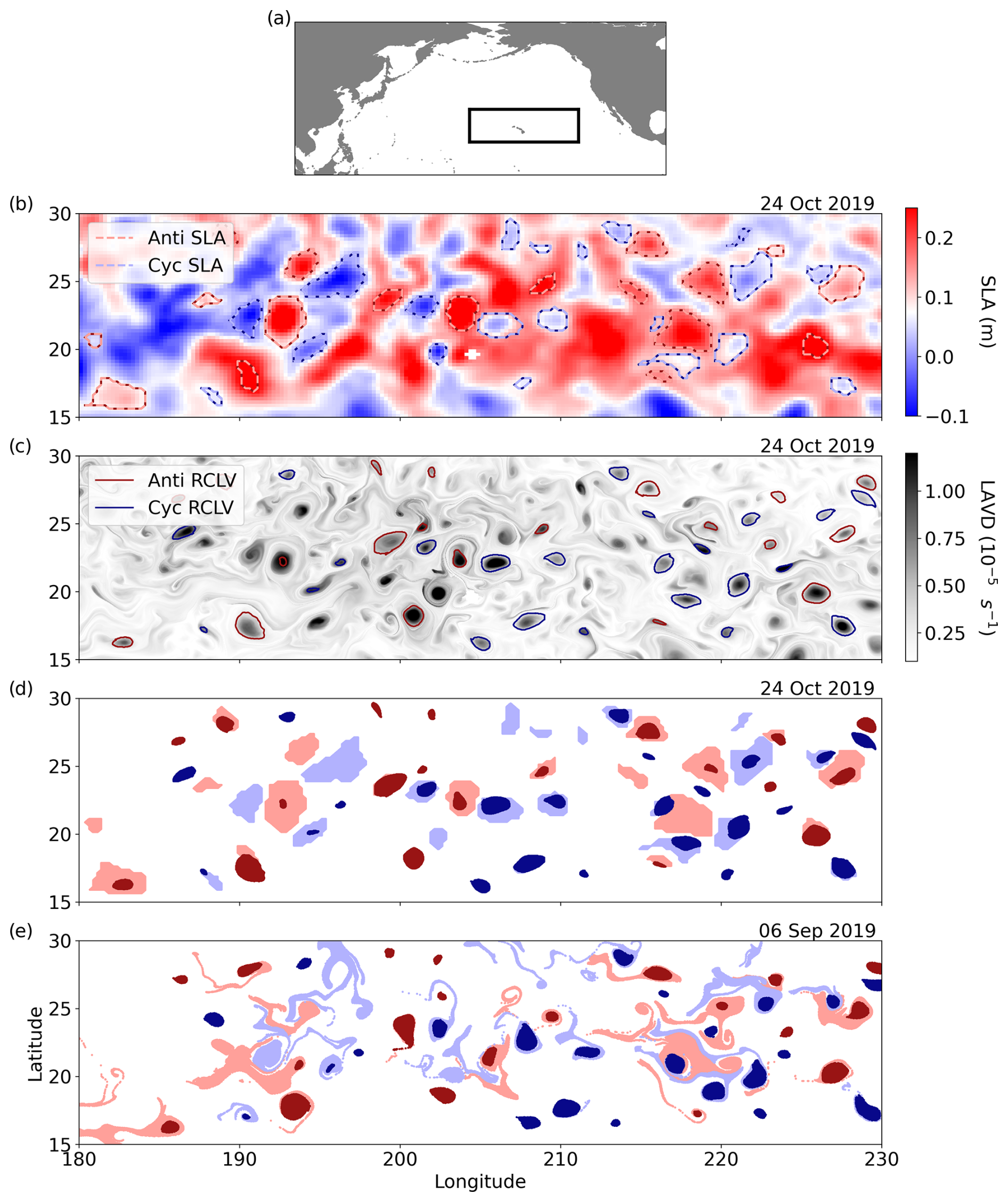
Figure 1 Maps of the study domain and eddy identification from a single time step. (a) The North Pacific Ocean and a black box outlining the bounds of the study domain. (b) The SLA field on 24 October 2019, with the SLA-derived eddy bounds outlined with dotted lines. (c) The Lagrangian-averaged vorticity deviation (LAVD) field on 24 October 2019 and the derived rotationally coherent Lagrangian vortex (RCLV) boundaries outlined with solid lines. (d) The initialization of Lagrangian particles in each type of eddy on 24 October 2019. The light red (blue) is associated with anticyclonic (cyclonic) SLA eddies, and the dark red (blue) is associated with anticyclonic (cyclonic) RCLVs. The darker color is plotted when the SLA eddy and RCLV zones overlap. (e) The 32 d backward-in-time locations (i.e., on 6 September 2019) of the Lagrangian particles that were initialized in (d).

We used the Copernicus Marine Service (CMEMS) $\mathrm{1}/\mathrm{4}$° daily satellite geostrophic current and SLA gridded fields (CMEMS, 2020) for Eulerian and Lagrangian eddy identification. We obtained the 8 d average satellite chl a Ocean Color Climate Change Initiative (OC-CCI) product with a spatial resolution of 4 km at the Equator (Sathyendranath et al., 2019). The CMEMS and OC-CCI products spatiotemporally interpolate information from all available altimeter and ocean color products, respectively. We note that the numerical treatment of these data affects the accuracy of mesoscale feature tracking (Capet et al., 2014; Ballarotta et al., 2019) and the detection of their chl a signatures.

2.1 Eddy atlases

2.1.1 Eulerian eddy atlas

We used the OceanEddies algorithm to generate an Eulerian eddy atlas from the satellite SLA (Faghmous et al., 2015). This flexible software allowed us to set parameters aligned as closely as possible to the Lagrangian eddy atlas, described in the next section. OceanEddies identifies an eddy boundary as the outermost closed contour containing a single SLA extremum and tracks the movement of features over time. We required eddies to have a minimum detectable lifespan of 32 d and boundaries to contain 12 or more $\mathrm{1}/\mathrm{4}$° grid cells. The smallest SLA eddy from this criteria has an area of 8048 km² with a radius of approximately 50 km, consistent with the Rossby radius of deformation in the domain (Chelton et al., 1998). We set the eddy disappearance parameter to 3 d, which accounts for noise in the gridded SLA satellite product that could cause premature termination of eddy tracking (Chelton et al., 2011b). For the ensuing analysis, we reduced the temporal resolution of the SLA atlas to an 8 d frequency, synchronized with the OC-CCI chl a product. From 2 decades of data, we tracked 6846 unique SLA eddies (or 52 553 observations resolved every 8 d), including 3322 anticyclones characterized by SLA maxima and 3524 cyclones characterized by SLA minima. The median lifespan of the tracked SLA eddies was 55 d, but one survived as long as 503 d in this domain.

2.1.2 Lagrangian eddy atlas

We expanded upon the Lagrangian eddy atlas developed by Jones-Kellett and Follows (2024) to identify and track coherent vortices. They derived eddy boundaries from the Lagrangian-averaged vorticity deviation (LAVD), a measure of the integrated vorticity experienced by a Lagrangian particle over the timescale of interest (Haller et al., 2016). First, the LAVD for Lagrangian particles was mapped to their gridded initialization locations. Closed contours surrounding a local maximum in the resulting LAVD field were assumed to be fluid sets in rigid-body rotation, referred to as rotationally coherent Lagrangian vortices (RCLVs) (Haller et al., 2016; Tarshish et al., 2018). These steps were performed for Lagrangian particle simulations re-initialized every 8 d from 2000 through 2019 (synchronized with the OC-CCI 8 d chl a product; Fig. B1) and advected for 32 d backward-in-time. After RCLV contours were discretely identified every 8 d, the features were tracked between time steps and linked with an eddy identification number if they encompassed the same core fluid mass. This method requires any given Lagrangian particle to be part of the coherent structure for 32 d but does not require it to be retained in the feature for the entire lifespan of the tracked eddy. Thus, eddy growth during their formations and shrinking as they decay are accounted for. The Lagrangian trajectory analysis required parallel processing and 3.4 Tb of storage, so a limitation of this method compared to Eulerian ones is the large computational expense.

Young developing eddies can harbor large biological anomalies (Gaube et al., 2013). So, to holistically evaluate how eddy trapping alters chl a concentration, it was important to resolve RCLV genesis. The RCLV atlas presented by Jones-Kellett and Follows (2024) (Version 1: Jones-Kellett, 2023a) included features that were coherent for at least 32 d, so the youngest eddy phases captured in Version 1 are already 32 d old. Here, we followed the Lagrangian particles contained within each 32 d old RCLV backward-in-time to resolve the feature geneses. Following the existing atlas resolution of 8 d time steps, we drew closed contours to encompass the particle sets at ages 24, 16, and 8 d (Fig. B2). The quality control steps conducted for the extended RCLV atlas are detailed in the decision tree in Fig. B3. This new “Version 2” of the atlas contains 11 855 unique RCLVs (or 75 445 polygons resolved every 8 d), including 5592 anticyclones characterized by a negative sign of relative vorticity and 6263 cyclones characterized by a positive sign of relative vorticity. The median lifespan of the RCLVs is 40 d, and the maximum is 413. RCLVs typically persist for shorter timescales than their SLA eddy counterparts in this domain, except in the lee of the Hawaiian Islands (Jones-Kellett and Follows, 2024). Version 2 of the NPSG RCLV atlas is publicly available, distributed by Simons CMAP at https://simonscmap.com/catalog/datasets/RCLV_atlas_version2 (last access: 11 July 2024) (Jones-Kellett, 2024).

2.2 Eddy categorization

When comparing RCLVs and SLA eddies from concurrent atlases, it is notable that some features are observed with only one method, whereas many are detected with both (Liu et al., 2019). The boundaries of eddies identified in both datasets (i.e., “overlapping”) can differ considerably, and overlapping RCLVs tend to be smaller in size (Liu et al., 2019; Liu and Abernathey, 2023) and nested within a larger SLA eddy boundary (Jones-Kellett and Follows, 2024). For this analysis, we categorized each pixel from the satellite chl a fields as “background” (i.e., outside-eddy) or inside an eddy. In-eddy pixels can be within an SLA eddy, RCLV, or both. Pixels inside an SLA eddy boundary but not an RCLV are referred to as “SLA excluding RCLV”. This includes the dispersive regions of overlapping eddies and the entirety of SLA eddies that do not contain a coherent structure (i.e., only the light-colored particles in Fig. 1d and e). The “SLA eddy” category includes all pixels within an eddy boundary irrespective of whether it contains an RCLV. This classification is directly comparable to studies that invoke Eulerian eddy identification methods. The “RCLV” category includes any particle in a coherent vortex, whether or not it overlaps with an SLA eddy (i.e., only the dark-colored particles in Fig. 1d and e). Figure 1d and e illustrate the considerable difference in the trapping nature of the respective eddy identification methods. The dark blue and red particles initialized in the RCLVs remain as visually coherent patches after the 32 d backward-in-time advection, whereas the light-colored particles are filamented and widely dispersed.

2.3 Chlorophyll anomaly definitions

The climatological chl a anomaly is a temporal, Eulerian metric defined as

$$\begin{array}{}\text{(1)}& \mathit{\delta }{c}_{\mathrm{clim}}(x,y,t)=c(x,y,t)-{\displaystyle \frac{\mathrm{1}}{M}}\sum _{t^{\prime }=\mathrm{0}}^{M}c(x,y,t^{\prime }),\end{array}$$

where $c(x,y,t)$ is the chl a at location (x, y) and time t. The second term describes the 2000 through 2019 average chl a in the month corresponding to the date t (i.e., the monthly climatology shown in Fig. B4), such that M is the number of data points available for that month. A positive δc_clim indicates that chl a is higher than the average at that location in the given month. We used δc_clim to isolate the mesoscale-driven changes in chl a that are distinct from the seasonal cycle.

We define the relative difference in the eddy and background probability density distributions of δc_clim as

$$\begin{array}{}\text{(2)}& f\left(\mathit{\delta }{c}_{\mathrm{clim}}\right)={\displaystyle \frac{p_{\mathrm{E}}\left(\mathit{\delta }{c}_{\mathrm{clim}}\right)-p_{\mathrm{B}}\left(\mathit{\delta }{c}_{\mathrm{clim}}\right)}{p_{\mathrm{B}}\left(\mathit{\delta }{c}_{\mathrm{clim}}\right)}},\end{array}$$

where p_E(δc_clim) is the density distribution of the climatological chl a anomalies in an eddy type and p_B(δc_clim) is the density distribution of anomalies in the background ocean. This metric quantifies whether a given δc_clim is more likely to be observed in randomly sampled waters of the background ocean or an eddy: f(δc_clim)=1 corresponds to a 100 % increase in the density of observations of δc_clim in the eddy compared to the background. Figure 2 shows an idealized, illustrative example where the probability density distribution of δc_clim for an eddy type (in purple) is shifted more positively compared to the background (in gray), yielding f(δc_clim)>0 for all positive values and f(δc_clim)<0 for all negative values. Data in each quadrant of the f(δc_clim) plots can be interpreted as follows.

• Q1: Positive anomalies are more likely to be observed in an eddy than in the background ($f(+\mathit{\delta }{c}_{\mathrm{clim}})>\mathrm{0}$).

• Q2: Negative anomalies are more likely to be observed in an eddy than in the background ($f(-\mathit{\delta }{c}_{\mathrm{clim}})>\mathrm{0}$).

• Q3: Negative anomalies are less likely to be observed in an eddy than in the background ($f(-\mathit{\delta }{c}_{\mathrm{clim}})<\mathrm{0}$).

• Q4: Positive anomalies are less likely to be observed in an eddy than in the background ($f(+\mathit{\delta }{c}_{\mathrm{clim}})<\mathrm{0}$).

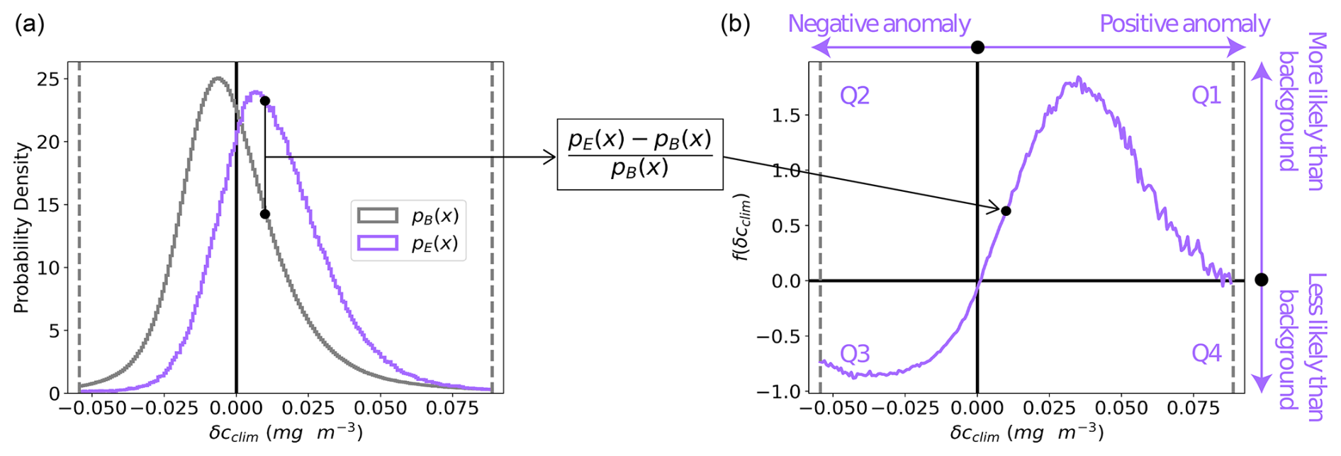
Figure 2 A schematic demonstration of the transformation of the probability density distribution of the climatological chl a anomaly in an eddy type (p_E(δc_clim)) to its relative difference from the background (f(δc_clim); Eq. 2). In panel (a), artificial data representing the background are plotted in gray and an artificial eddy type in purple. The vertical dotted lines represent the cutoffs at the 1st and 99th percentiles of the background probability density distribution. Panel (b) shows the relative difference between the eddy and background probability density distributions of δc_clim, demonstrating the difference in the likelihood of a given chl a anomaly to occur in the eddy type compared to the background ocean.

We define a local eddy-associated chl a anomaly used to analyze the evolution of blooms in individual features in Sect. 3.3,

$$\begin{array}{}\text{(3)}& \mathit{\delta }{c}_{\mathrm{loc}}=\underset{\mathrm{Inside}\mathrm{Eddy}}{\underbrace{{\displaystyle \frac{\mathrm{1}}{A_{\mathrm{in}}}}\underset{\mathrm{I}}{\oint }c(x,y)dI}}-\underset{\mathrm{Outside}\mathrm{Eddy}}{\underbrace{{\displaystyle \frac{\mathrm{1}}{A_{\mathrm{out}}}}\underset{\mathrm{O}}{\oint }c(x,y)dO}},\end{array}$$

where I is the eddy polygon with area A_in, and O is the annulus (the polygon from the boundary of the eddy to a circle with twice the eddy radius) with area A_out. The first term of Eq. (3) is the average chl a inside the eddy, and the second is the average in the immediate surroundings. A positive δc_loc indicates that the mean chl a concentration is higher within the eddy than outside. Since this metric follows an eddy through time and space, it can be considered a Lagrangian chl a anomaly.

2.4 Confidence intervals

Tests of statistical significance are uninformative when comparing the distributions of large datasets because the p value converges to zero (e.g., Lin et al., 2013), as is the case here when aggregating 2 decades of satellite chl a data. Alternatively, we computed confidence intervals for f(δc_clim) (as suggested in Hubbard and Armstrong, 2006) using a nonparametric bootstrapping method (Efron, 1979). First, the numpy.random.choice( ) Python function was used to randomly resample the δc_clim datasets with replacement a number of times equivalent to the original sample size (sample sizes range from 411 546 to 25 960 826; Tables C2 and C3). “With replacement” means that each data point could be sampled in every draw, even if previously chosen. Next, we calculated f(δc_clim) from the probability density distribution of the bootstrap dataset. These steps were repeated 1000 times for each eddy type. Finally, we estimated 95 % confidence intervals for every δc_clim value from the 2.5 to 97.5 percentiles of the 1000 bootstrap f(δc_clim) distributions.

3 Results

3.1 Gyre-scale chlorophyll signatures of eddy trapping

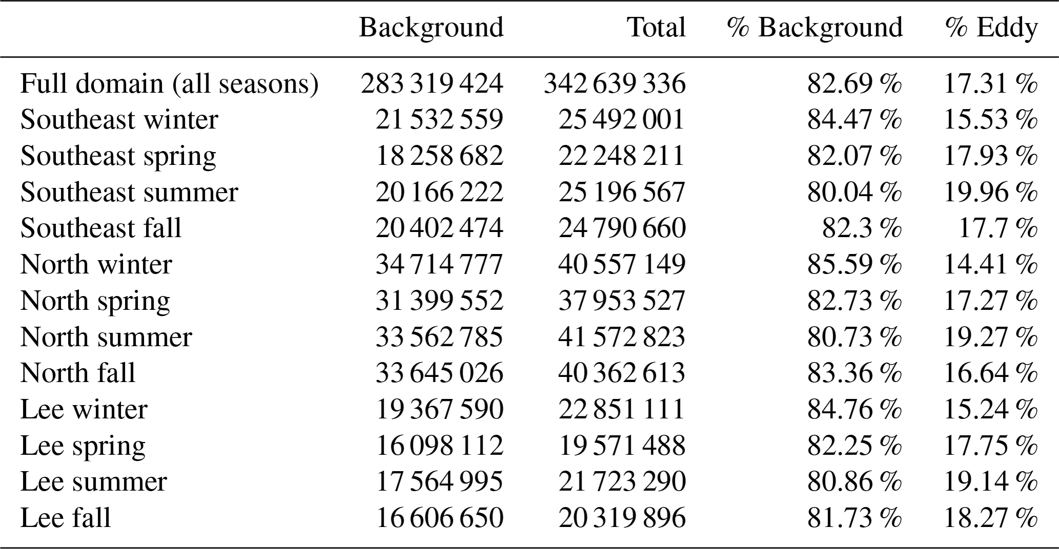
To isolate eddy-driven changes in chl a, we subtracted the climatological seasonal cycle at each grid cell in the satellite chl a fields (Eq. 1), yielding climatological chl a anomaly fields from 2000 through 2019. We binned the chl a anomaly data by the categorizations described in Sect. 2.2: anticyclonic RCLV, anticyclonic SLA eddy, anticyclonic SLA excluding RCLV, cyclonic RCLV, cyclonic SLA eddy, cyclonic SLA excluding RCLV, or background. Of the chl a measurements, 82.7 % were collected in the background ocean (i.e., outside of all eddy types; n=283 319 424) while 17.3 % were in an Eulerian and/or Lagrangian eddy (n=59 319 912; Table C4).

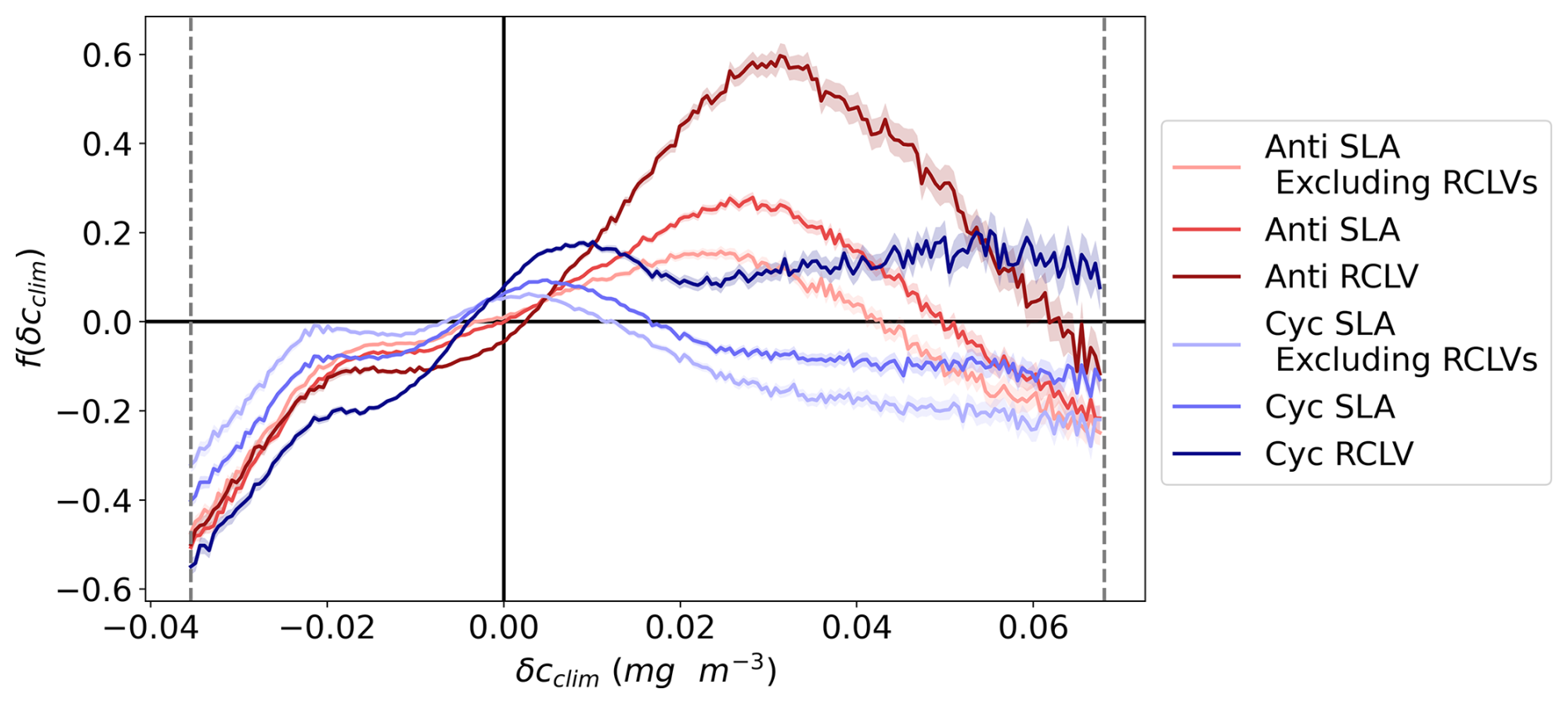
Figure 3 The cumulative chlorophyll signature of NPSG eddies, categorized by the lateral trapping behavior. f(δc_clim) is the relative difference in the eddy probability density distributions from the background (Eq. 2), including data from the 1st to 99th percentiles (labeled with the vertical dotted gray lines). A positive f(δc_clim) indicates that the given δc_clim is more likely to be observed in an in-eddy water parcel than in the background. The anticyclones are plotted in red and cyclones in blue, where the darkest colors represent the chlorophyll within rotationally coherent Lagrangian vortices (RCLV), and the lightest represent the chlorophyll of the leakiest eddy zones (SLA excluding RCLV). The shaded regions represent the 95 % confidence intervals. Figure B5 shows the corresponding probability density distributions of δc_clim.

3.1.1 Anticyclonic eddies

NPSG anticyclonic eddies tend to contain waters with elevated chl a relative to the non-eddy background. Figure 3 plots f(δc_clim) (Eq. 2), or the likelihood of observing a given chlorophyll anomaly by eddy type relative to the background, with the anticyclones in red. Negative values of δc_clim are less likely to occur within all anticyclonic eddy types than in the background. Positive chl a anomalies are more common in all anticyclones compared to outside eddies, except at extremely high values. More specifically, anomalies over 0.049 mg m⁻³ occurring in SLA eddies and 0.061 mg m⁻³ in RCLVs are rarer than in the background. Therefore, anticyclones elevate chl a but only up to a threshold magnitude. To contextualize these anomalies, the average surface chl a concentration in the NPSG from 2000 to 2020 was 0.068 mg m⁻³ (although this varies regionally and seasonally (Fig. B4)). Thus, anticyclonic RCLVs are 59.7 % more likely than the background ocean to contain chl a blooms with concentrations roughly 1.5 times the average (δc_clim=0.031 at max(f)=0.597) but are not likely to double the average concentration.

Of satellite pixels co-located within anticyclonic SLA eddies, 21 % are also contained within an RCLV (Table C2). In other words, only one-fifth of the aggregate SLA eddy area is strictly coherent for 1 month or longer. The leaky zones of SLA eddies, or SLA excluding RCLVs, are more likely than the background to contain positive δc_clim, but only up to 0.043 mg m⁻³. This threshold is lower than for RCLVs and the all-inclusive SLA eddy categories, indicating that the highest chl a anomalies associated with SLA eddies are largely contained within nested Lagrangian coherent structures.

3.1.2 Cyclonic eddies

Cyclonic eddies alter surface chlorophyll in the NPSG compared to outside-eddy waters with signatures that differ in some ways from anticyclones (shown in blue in Fig. 3). Negative climatological anomalies are less likely to occur in all cyclonic eddy types than in the background ocean and the least likely in RCLVs, as was the case for anticyclones. Cyclonic RCLVs are up to 20.4 % likelier to have positive chl a anomalies than the non-eddy background ocean. In contrast to anticyclonic RCLVs, cyclonic coherent structures elevate or maintain chl a at very high anomaly values. Yet, moderately positive δc_clim are less likely to occur in cyclones compared to anticyclones. Other than for very modest values (<0.016 mg m⁻³), SLA cyclones are less likely to have positive chl a anomalies than the background.

Of satellite pixels in cyclonic SLA eddies, 23 % are also contained within an RCLV (Table C3) and are not included in the “SLA eddies excluding RCLVs” category. The leakiest components of SLA eddies are less likely than the background to contain a positive chlorophyll anomaly greater than 0.016 mg m⁻³. Hence, in both cyclones and anticyclones, coherent structures within SLA eddies are more often associated with positive chl a anomalies than the background.

3.1.3 Gyre-scale summary

RCLVs of both polarities are less likely to have negative chl a anomalies and more likely to have positive anomalies compared to the background and SLA eddies. Fewer positive chl a anomalies are attributed to SLA eddies when excluding nested RCLVs than to all-encompassing SLA eddies. Together, these data support the hypothesis that coherent features trap and maintain phytoplankton blooms which are instead rapidly diluted via lateral mixing in less coherent eddies.

3.2 Regional and seasonal subdomains

Here we explore the sub-regional and seasonal variations in the chl a signature of eddy trapping in the NPSG. Subdomains of contrasting mesoscale eddy activity by polarity are revealed in Fig. 4a by the eddy polarity probability (P) (Chaigneau et al., 2009), defined as

$$\begin{array}{}\text{(4)}& P(x,y)={\displaystyle \frac{F_A(x,y)-F_C(x,y)}{F_A(x,y)+F_C(x,y)}}.\end{array}$$

F_A(x,y) (F_C(x,y)) is the number of times the pixel at location (x, y) was inside an anticyclone (cyclone) from 2000 through 2019. Anticyclonic eddy polarity is more frequent than cyclonic when P>0. There is more anticyclonic activity north of latitude 23° N, cyclonic domination to the east of Hawai`i, and signatures of the lee eddies to the west of the islands. We found distinct and sometimes dramatic differences in the chl a responses between anticyclonic and cyclonic eddies of the north, southeast, and Hawaiian lee provinces. The monthly chl a climatologies vary moderately by region (Fig. B8).

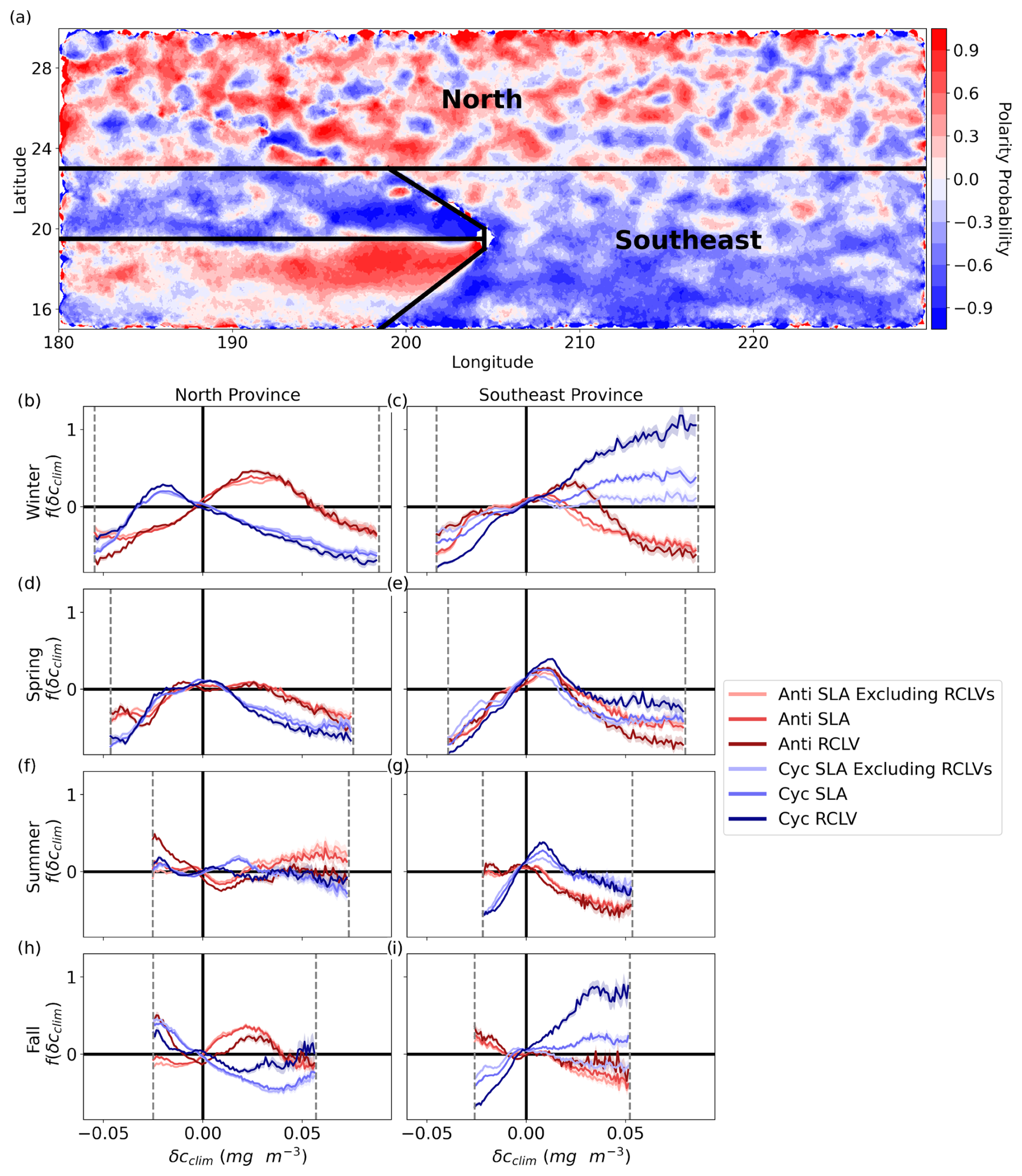
Figure 4 Chl a signature of north and southeast NPSG eddies. (a) RCLV polarity probability (Eq. 4). Red (blue) indicates that anticyclones (cyclones) are more common at the location. The black lines delineate the provinces defined in this study. (b–i) The relative difference in the probability density distribution of the eddy-associated climatological chl a anomaly (δc_clim) from the background (f(δc_clim)) for each eddy type. Each row corresponds with a season such that winter includes December through February, and so on. The dotted gray lines show the 1st to 99th percentiles of the background ocean for the given season and region. These cutoff boundaries ensure sufficient data underlie the calculations of f(δc_clim). The shaded regions represent the 95 % confidence intervals. Figures B6 and B7 show the corresponding probability density distributions of δc_clim.

3.2.1 Northern eddies

In the winter and spring (Fig. 4b and d), there are no substantial disparities in chl a anomalies between northern RCLVs and SLA eddies. However, some differences emerge in the summer and fall (Fig. 4f and h), indicating an influence of eddy trapping on chlorophyll patchiness in the surface ocean. Although collectively across the gyre there is an overall increase in positive chl a anomalies within RCLVs compared to SLA eddies (Sect. 3.1), this pattern does not necessarily hold in the north province. This emphasizes the need for focused regional and seasonal analyses and illustrates the complexity of biogeochemical response to mesoscale eddies.

Anticyclones

Occurrences of positive δc_clim are up to 46.5 % more common in all types of anticyclones (represented by the red curves in Fig. 4) than in the background during the northern winter, up to approximately 0.056 mg m⁻³. This aligns with observations of elevated surface chl a in wintertime anticyclonic eddies in subtropical gyres globally (Dufois et al., 2016). However, the average chl a concentration is highest in the northern winter, so the northern anticyclones are likely to elevate chl a by relatively similar quantities as in the fall: up to 56.5 % of average concentrations in the fall versus 59.9 % in the winter (Fig. B8b). During the summer and fall, anticyclonic RCLVs, but not SLA eddies, are likelier to have a negative chl a anomaly than the background. This suggests that, in some cases, limited dilution in RCLVs yields a local depletion of chl a. On the other hand, SLA anticyclones have f(δc_clim)>0 for more positive values of δc_clim than RCLVs in the summer and fall.

Cyclones

Northern cyclonic eddies (represented by the blue curves in Fig. 4) generally exhibit fewer positive chl a anomalies than the background across all seasons except the summer, where the distributions resemble the background ocean. Moreover, cyclonic RCLVs are less prone to have positive anomalies than SLA eddies in all seasons except for the fall, indicating that eddy trapping does not typically heighten chlorophyll levels in cyclonic features of the northern province. In the winter and fall, northern cyclones of all types are likelier to display negative δc_clim values than the background.

3.2.2 Southeastern eddies

The probability density distributions of δc_clim exhibit substantial disparities between RCLVs and SLA eddies within the southeast province, especially in cyclones, for all seasons (Fig. 4c, e and i) except for the summer (Fig. 4g). Notably, anticyclones are much less prevalent than cyclones in the southeast province, so observations of anticyclones in this region play a small role in their overall effects in the gyre shown in Fig. 3. Conversely, the high frequency of cyclones in the southeast contributes largely to the data in Fig. 3.

Anticyclones

Southeastern anticyclonic eddies have distinct relationships with chl a compared to their northern counterparts. In winter, anticyclonic RCLVs are more likely to exhibit positive δc_clim values than the background ocean, but up to a lower threshold (0.037 mg m⁻³) than in the north (0.054 mg m⁻³). Unlike in the north, wintertime SLA anticyclones have distributions more akin to the background. During spring, all anticyclonic eddy types are likelier than the background to have small positive δc_clim, up to 0.024 mg m⁻³. However, positive chl a anomalies in southeastern anticyclones are unlikely in summer and fall, with all types in the fall showing a propensity for negative anomalies. This differs from the northern fall where positive δc_clim values are found in anticyclonic eddies and only RCLVs are likely to have negative anomalies.

Cyclones

Cyclonic δc_clim distributions in the southeast province differ greatly from the north. All cyclone types exhibit f(δc_clim)<0 for negative δc_clim throughout the year, suggesting that cyclones consistently enhance chl a in this region. During fall and winter, cyclonic RCLVs are much likelier than both the background and SLA eddies to have positive δc_clim, especially at high values. For example, wintertime southeastern cyclonic RCLVs are 118.3 % more likely than the background to contain δc_clim=0.077 mg m⁻³, or a doubling of the background average chl a concentration (Fig. B8b). Because the chl a signatures of cyclonic SLA eddies excluding RCLVs are similar to the background, positive anomalies in the SLA eddies can be largely attributed to RCLVs nested within their bounds. Thus, eddy trapping plays a prominent role in elevating local chl a anomalies in cyclones of the southeast province.

Anomalies are rarer during spring and summer when southeastern cyclones are only more likely than the background to have positive δc_clim up to a threshold magnitude. This cutoff is 0.018 mg m⁻³ for cyclonic SLA eddies in the spring and 0.026 mg m⁻³ for RCLVs. In summer, it is 0.019 mg m⁻³ for SLA eddies and 0.021 mg m⁻³ for RCLVs. For context, the average chl a concentration in the southeast spring is 0.063 and 0.060 mg m⁻³ in the summer (Fig. B8b), so RCLVs are likely to enhance chl a by up 41.3 % and 35.0 % of spring and summer average concentrations, respectively.

3.2.3 Hawaiian lee eddies

The “Hawaiian lee eddies” are large, long-lived features that consistently form in the lee of the Hawaiian Islands (Fig. 5a). Anticyclones are generated by the shear instability between the eastward-flowing Hawaiian Lee Countercurrent and the westward-flowing North Equatorial Current (Calil et al., 2008; Yoshida et al., 2010; Liu et al., 2012). Lee cyclones are produced from wind stress curl anomalies due to trade wind blocking by the islands (Lumpkin, 1998; Dickey et al., 2008; Yoshida et al., 2010). The Hawaiian Lee Countercurrent to the south and the westward-flowing Hawaiian Lee Current to the north sustain the cyclonic vorticity, evident from bands in the sign of polarity probability to the west of the islands (Fig. 4a).

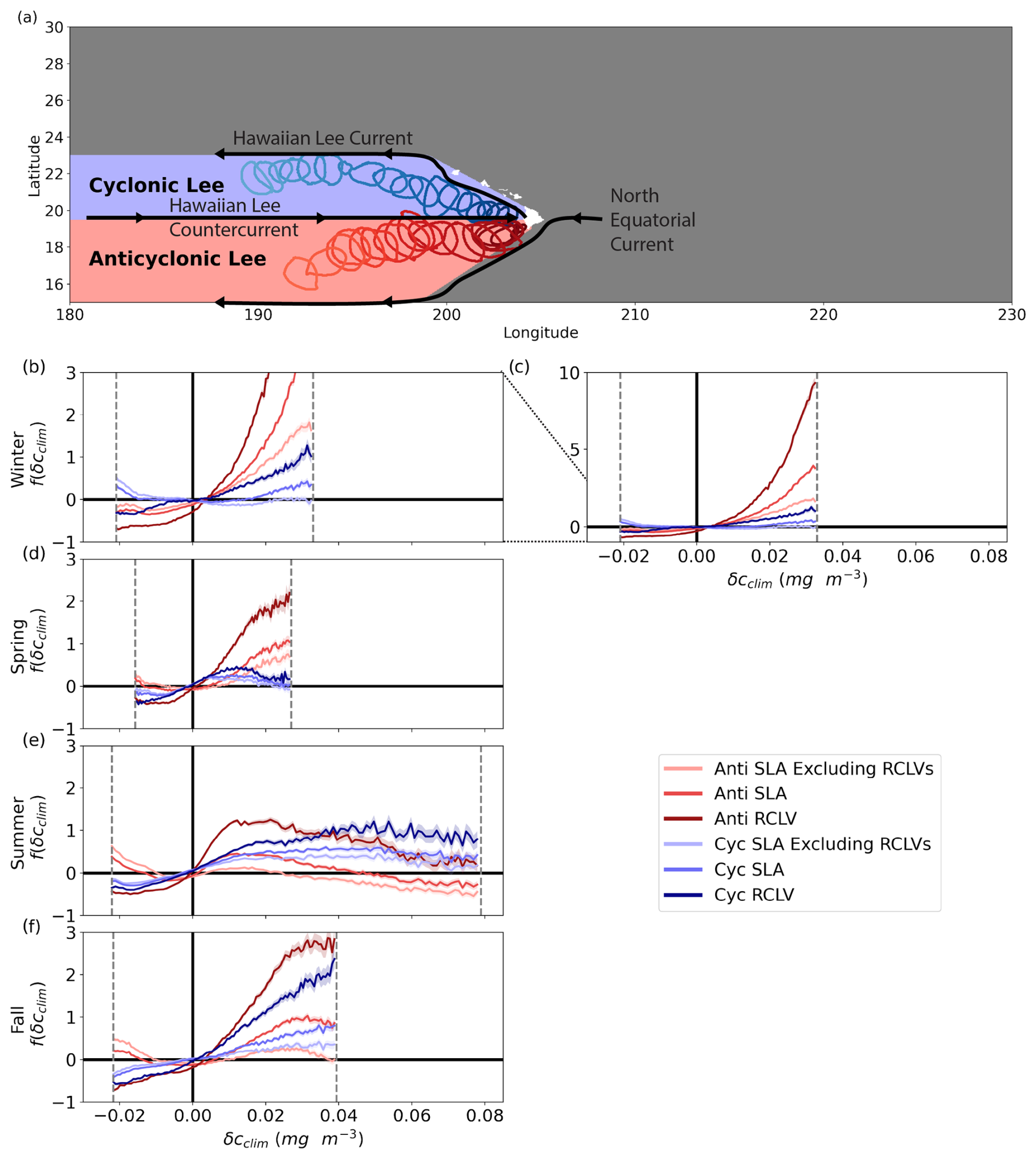
Figure 5 Chl a signature of Hawaiian lee eddies. (a) Schematic of the currents that sustain the Hawaiian lee eddies. The region dominated by anticyclones (cyclones) is red (blue). The boundaries of two RCLVs are plotted every 16 d to show the common propagation pathways westward from the islands, where the darker contours represent young eddies and the lighter represent old eddies. (b–f) The relative difference in probability density distributions of the climatological chl a (δc_clim) anomaly from the background (f(δc_clim)). The dotted gray lines show the 1st to 99th percentiles of the background ocean for the season and region. These cutoff boundaries ensure sufficient data underlie the calculations of f(δc_clim). The shaded regions represent the 95 % confidence intervals. Figure B9 shows the corresponding probability density distributions of δc_clim. Note that the y axis differs from Figs. 3 and 4 to accommodate larger values of f(δc_clim). Panel (c) includes the same information as (b) with a different y axis to expose the entirety of the curves.

RCLVs and SLA lee eddies of both polarities drive more positive chlorophyll anomalies than the background throughout the entire annual cycle (Fig. 5b–f), distinguishing them from features in the north and southeast provinces (Fig. 4). RCLVs of both polarities have more positive chl a anomalies than their corresponding SLA eddies and the background across all seasons. SLA eddies excluding RCLVs more closely resemble the background, highlighting the importance of trapping for locally enhancing the chl a signature of the Hawaiian lee eddies.

Although the chl a anomalies of the lee eddies are consistently positive, the magnitudes vary seasonally. In summer and fall, δc_clim distributions are similar between cyclones and anticyclones, whereas, during the winter and spring, anticyclones are much more prone to positive anomalies. Even the leakiest anticyclonic features host positive δc_clim on par with cyclonic RCLVs during these seasons. Wintertime anticyclonic RCLVs host the most extreme positive δc_clim compared to all other eddies in the domain. For example, they have a 933.0 % higher likelihood than the background ocean to contain δc_clim=0.032 mg m⁻³, or a 51.6 % increase in chl a concentration compared to the regional and seasonal average (Fig. B8). Summer and fall witness more negative anomalies of chl a in anticyclonic SLA eddies than in the background, suggesting that chl a can also be depleted in these features. This is only the case for cyclonic SLA eddies in the winter.

3.2.4 Regional summary

To summarize the regional variations, the signs of the chl a anomalies in anticyclones and cyclones differ in the northern NPSG, but there is little contrast between SLA eddies and RCLVs there. The role of dilution limitation via eddy trapping in this region is likely being counteracted by other biophysical interactions. In the southeast and the lee of the Hawaiian Islands, there are large differences between chl a anomalies in SLA and RCLV features, suggesting trapping plays an important role in maintaining chl a in the southern latitudes of the NPSG. This southern signature dominates the differences in chl a anomalies between SLA eddies and RCLVs in the collective gyre-scale analysis (Sect. 3.1).

3.3 Evolution of long-lived coherent eddies

Feature tracking in the RCLV atlas enables examination of chl a patches as they evolve through time as quasi-isolated systems. We address whether there is a common sequence or trend in chlorophyll anomalies in strongly coherent features as a function of eddy age. We hypothesized stronger anomalies in the early, growing phase, weakening with age, but the data reveal a more complex pattern.

We analyzed the in-eddy anomaly compared to the immediate surroundings, δc_loc (Eq. 3), as a function of age for the 245 RCLVs (109 anticyclones, 136 cyclones) that maintained coherency for 150 or more days. Figure 6a illustrates the consistent westward propagation of these features. Figure 6b shows the magnitudes of the local Lagrangian chlorophyll anomalies with age, separated by season and province. There is not a single consistent pattern of change in δc_loc with age, rather it depends on the region, season, and polarity, complementing the results of Sect. 3.2.

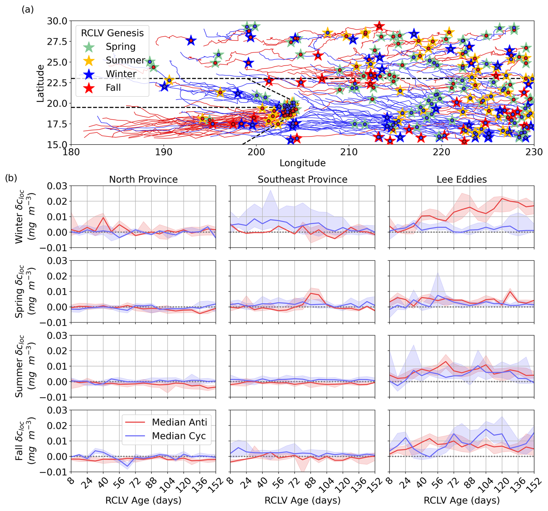
Figure 6 (a) Trajectories of the eddy centers for long-lived (150+ d) RCLVs from 2000 through 2019. The anticyclonic (cyclonic) eddy trajectories are in red (blue). The stars indicate the location of the eddy genesis and are color-coded by the birth season. The dotted black lines show the boundaries of the mesoscale provinces used for the analysis in this study. (b) Local chl a anomalies (δc_loc) in RCLVs with lifespans of 150+ d. Each column corresponds to a mesoscale-driven province and each row with the season. Anticyclonic (cyclonic) eddies are in red (blue). The solid lines show the median δc_loc by RCLV age, and the shaded areas are the ranges of the 25th to 75th percentiles.

RCLVs in the north have minimally altered chl a compared to their immediate surroundings except in wintertime anticyclones, which show some elevation relative to their surroundings early in their lifetimes. Southeastern cyclonic RCLVs foster heightened chl a relative to their surroundings in the winter and fall, and these anomalies decline with eddy age. Hawaiian lee cyclonic and anticyclonic RCLVs have substantially enhanced chl a relative to their surroundings throughout their entire lifetimes. There is a notable trend in wintertime lee eddy anticyclones, where δc_loc monotonically increases with eddy age.

4 Discussion

Harnessing the temporal and spatial coverage of satellite observations, we compared Lagrangian (RCLV) and Eulerian (SLA) eddy atlases to differentiate the biological signatures of coherent eddies, dispersive eddies, and the background ocean in the NPSG over 2 decades. Aggregated to the gyre-scale, more positive climatological chl a anomalies are observed in RCLVs than in SLA eddies or outside-eddy waters (Fig. 3), supporting our hypothesis: coherent features maintain eddy-driven anomalies more intensely, and for longer, than their leaky counterparts due to the limitation of lateral dilution. However, this domain-wide response largely reflects the behavior of the southeastern (Fig. 4) and Hawaiian lee eddies (Fig. 5) and is not evident in the northern NPSG (Fig. 4). We tested whether there is a pattern in the intensity of chl a anomalies as a function of age in the longest-lived RCLVs, finding this also depended on the region, season, and polarity (Fig. 6). There was often no trend, but the strongest observed pattern was linearly increasing positive anomalies of chl a concentrations in Hawaiian lee anticyclones over their lifetimes.

Our results reveal a complex relationship between surface chl a concentrations and Lagrangian eddy trapping, with close coupling to the seasonal cycle and eddy location within the subtropical gyre. Here we discuss the potential mechanisms of this variability, the implications of these results on interpretations of eddy-driven biogeochemical changes, and comment on the nonlinearity parameter (a metric historically used to estimate eddy coherency). Lastly, we suggest topics worthy of future investigation and limitations of the satellite observations.

4.1 Regional variations and mechanisms

Positive anomalies are equally or more likely to occur in northern SLA anticyclones compared to in RCLVs during winter, summer, and fall (Fig. 4); this suggests that the net population growth rate is higher in SLA eddies to counteract or negate the chl a accumulation fostered by trapping. This may occur if lateral dilution drives higher growth rates (Ser-Giacomi et al., 2023) or reduces the grazing pressure (Lehahn et al., 2017). Other potential mechanisms that could drive this pattern include increased vertical mixing associated with submesoscale filaments on SLA eddy edges (Calil and Richards, 2010; Peterson et al., 2011; Mahadevan, 2016; Liu et al., 2017; Wang et al., 2018; Guo et al., 2019), eddy–eddy interactions (Guidi et al., 2012), wind interactions (Gaube et al., 2013, 2015), or the horizontal advection of chlorophyll or nutrient-rich waters into the eddy interior (Kuwahara et al., 2008; Nencioli et al., 2008; Xu et al., 2019).

Some RCLVs have more negative chl a anomalies than the background, including both polarities in the northern fall, wintertime cyclones in the north, anticyclones in the northern summer, and southeastern anticyclones in the fall (Fig. 4). Low chl a concentrations can result from deeper density surfaces in anticyclones that decrease the nutrient supply or high rates of phytoplankton mortality. In the interior of cyclones, phytoplankton cells may decrease their chlorophyll-to-carbon ratio if light availability increases (Geider, 1987; Macintyre et al., 2000) from shoaling isopycnals. In an RCLV where lateral dilution is minimized, negative anomalies are expected to be preserved longer than in SLA eddies because the chl a deficit is shielded from mixing with surrounding waters. However, negative anomalies occur more often within SLA eddy boundaries than their RCLV counterparts in some seasons in the Hawaiian lee eddy province (Fig. 5) and in cyclones in the northern fall (Fig. 4h). This could occur if the grazing pressure is higher on eddy edges than in their coherent centers (Froneman and Perissinotto, 1996; Goldthwait and Steinberg, 2008; Godø et al., 2012; Schmid et al., 2020) or if the eddy zone detected from the SLA is too liberal.

The Hawaiian lee eddies consistently form close to land, making them accessible for shipboard studies, and accordingly, the lee cyclones in particular have been heavily sampled. Though considered “model systems” for ocean eddies by some studies (Falkowski et al., 1991; Olaizola et al., 1993; Bidigare et al., 2003; Benitez-Nelson et al., 2007), we find that the lee eddies are not representative of eddies in the surrounding gyre. Hawaiian lee eddies of all types elevate chl a more than any other subdomain, even compared to features with similar lateral trapping capabilities. This is consistent with reports of dissimilar biogeochemical responses to eddies between Station ALOHA and the lee of Hawai`i (reviewed in Appendix A). The lee eddies of either polarity may act as carriers of blooms stimulated by the “island mass effect” (Hasegawa et al., 2009; Cardoso et al., 2020), where the coastal upwelling of subsurface nutrients or run-off from islands acts as fertilizer that enhances chl a concentrations and marine primary production (Doty and Oguri, 1956; Messié et al., 2020). This effect has been recognized in the lee of the Hawaiian Islands (Gilmartin and Revelante, 1974; Messié et al., 2022; Feloy et al., 2024), but separating its influence from other eddy-driven phytoplankton stimulants is challenging. For example, the high angular velocities of the lee cyclones may support more extreme isopycnal doming and eddy pumping of nutrients compared to eddies generated to the north or southeast of the islands (Friedrich et al., 2021). Ekman pumping from eddy–wind interactions likely drives blooms in the anticyclonic lee eddies (Gaube et al., 2014, 2015), consistent with our finding that chl a is most elevated in wintertime Hawaiian lee anticyclones, with trapping further enhancing local concentrations (Fig. 5) that linearly increase over their long lifetimes (Fig. 6). Nitrogen-fixing diazotroph blooms could also contribute to elevated chl a in the lee anticyclones, as found in a regional model study (Friedrich et al., 2021) and similarly observed in anticyclones north of Hawai`i (Church et al., 2009; Fong et al., 2008; Dugenne et al., 2023; Wilson et al., 2019; Cheung et al., 2020). However, these observations were primarily in the summer, which is the season with the least extreme likelihood of enhanced satellite chl a compared to the background ocean (Fig. 5e). In situ investigations of microbial communities in lee anticyclones are currently lacking but may be necessary to understand possible seasonal variations in plankton groups that contribute to increased chl a in these features.

4.2 Implications of the results

The observed variability in eddy trapping and chl a anomalies complicates estimates of the impact of subtropical gyre eddies on biogeochemical cycles. It is typical of in situ studies to have low sample sizes, identify eddy boundaries from an Eulerian method such as the SLA, and not characterize the trapping properties of features in a Lagrangian manner. In this study, only 22 % of SLA eddy-affiliated chl a observations are also within an RCLV (Tables C2 and C3), so it is more likely for in situ NPSG samples to be collected within dispersive eddy zones than coherent cores without a targeted approach. Since SLA eddies are found to alter chl a in some regions and seasons, the biogeochemical impacts of leaky eddies may be underestimated because mixing with surrounding waters can quickly dilute in-eddy concentrations. Furthermore, many studies compare “in eddy” and nearby “outside eddy” conditions to quantify eddy-driven biogeochemical anomalies. However, altered waters that leave the SLA eddy bounds may act to change nearby background concentrations, resulting in an underestimation of the eddy impacts. Understanding elevated chl a in RCLVs is also nontrivial because, at any given life stage, a coherent eddy could passively advect a phytoplankton patch or actively stimulate growth via vertical processes (Calil and Richards, 2010; Jönsson et al., 2009; Hernández-Carrasco et al., 2018). Distinguishing active and passive plankton dynamics in eddies is essential to quantify mesoscale contributions to primary production (Jönsson et al., 2011; Jönsson and Salisbury, 2016). We encourage future studies to consider the Lagrangian trapping strengths and advective histories of sampled eddies to support such biogeochemical interpretations.

4.3 A comment on the nonlinearity parameter

Many studies invoke the nonlinearity parameter, or the ratio of the eddy rotational to translation speed, to determine the trapping strength of SLA eddies. However, we found the nonlinearity parameter of SLA eddies (as computed by Chelton et al. (2011b)) poorly predicts Lagrangian eddy trapping and eddy-associated chl a anomalies. The nonlinearity parameter decreases with latitude in our domain (Fig. B10) and globally (Chelton et al., 2011b), which implies that eddy trapping should have a stronger influence on localizing chl a in the north. In direct opposition to this assumption, surface chl a anomalies are often more distinct in RCLVs than SLA eddies in the southern latitudes (Fig. 7b). Furthermore, we found a negligible difference in the nonlinearity parameter for SLA eddies that overlapped with an RCLV (median =5.566) and SLA eddies that did not (median = 5.545). Of SLA eddies that did not have an RCLV, 99.2 % had a nonlinearity parameter > 1 in this dataset, the threshold commonly used to suggest eddy coherency (Flierl, 1981; Chelton et al., 2011b, a). Previous studies have shown that the nonlinearity parameter is not predictive of Lagrangian coherency for eddies in other regions, including the Agulhas leakage (Beron-Vera et al., 2013), Gulf of Mexico (Beron-Vera et al., 2019), East Australian Current (Cetina-Heredia et al., 2019), North Brazil Current (Andrade-Canto and Beron-Vera, 2022), and South China Sea (Liu et al., 2022). We also find that the nonlinearity parameter is insufficient to determine eddy trapping strength in the NPSG. Given the consistency of these findings across various oceanic systems, we do not recommend using the nonlinearity parameter criterion alone to infer effective eddy coherency without further testing. Although Lagrangian metrics are more involved and computationally expensive, they are frame independent and more informative.

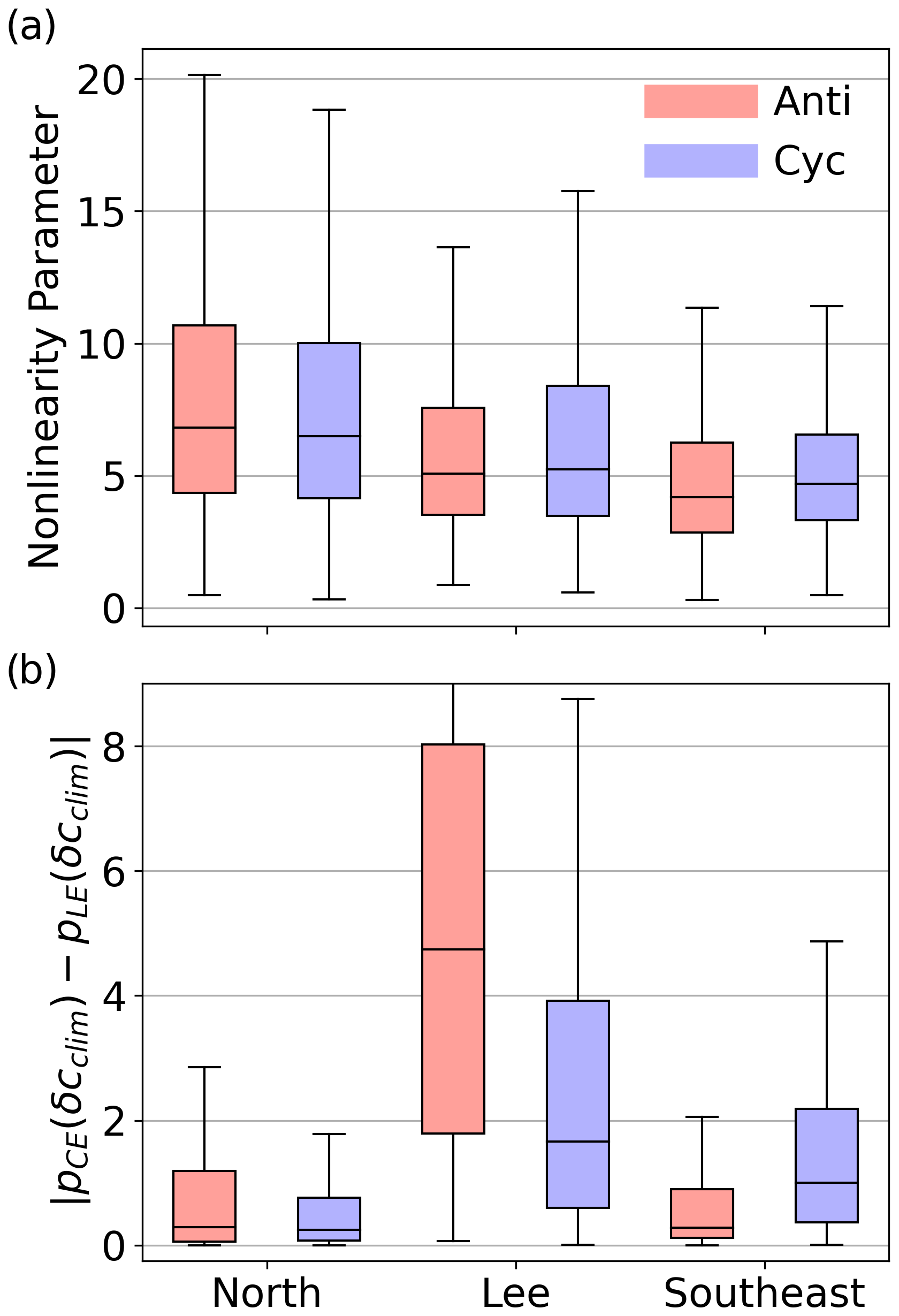
Figure 7 (a) Box plots showing the distribution of the nonlinearity parameter of SLA eddies by province and polarity. The provinces correspond to the delineations in Fig. 4a. The middle lines in the boxes are the medians of the data, the box edges represent the first and third quartiles, and the whiskers span the inter-quartile range. (b) The absolute difference in the likelihood of a given δc_clim to occur in coherent (p_CE) versus leaky eddies (p_LE). Larger values indicate that the chl a signature of eddy trapping is more distinct.

4.4 Future investigation and limitations

The difference in the polarity probability between the northern and southeast domains (Fig. 4a) remains unexplained, but there are analogous bands of dominating polarity across the global ocean (Dong et al., 2022). It is unclear whether the strong difference in the chl a signature of eddy trapping would differ across such bands in other regions or if the shift in the NPSG was coincidental. Furthermore, the north–south difference in the effect of eddy trapping on chlorophyll anomalies remains difficult to understand, but it may indirectly reflect large-scale patterns in the local environment. For example, background chl a concentrations are higher year-round in the northern latitudes of the NPSG compared to the southern, the euphotic zone is deeper to the north, and the mixed layer depths are deeper in the north than the southeast in the winter and have a higher seasonal amplitude. The nutricline shoals from the northern to the southern part of the gyre. These factors and the rich set of potential biophysical interactions described above in Sect. 4.1 make simple interpretations challenging. A physically and biologically well-resolved numerical simulation of the gyre could be used to attempt to tease apart the important dynamics but beyond the scope of this empirical study.

Satellite-observed changes in chl a at the mesoscale remain enigmatic concerning the underlying ecological dynamics because chlorophyll is not a direct measurement of phytoplankton biomass. For example, it is unknown whether elevated chl a in wintertime subtropical gyre anticyclones is due to increased productivity (Dufois et al., 2016) or changes in the cellular chlorophyll-to-carbon ratio due to photoacclimation (Cornec et al., 2021; He et al., 2021; Strutton et al., 2023). While both can be true (Su, 2021), higher fish catch occurs in anticyclones than cyclones around the Hawaiian Islands (Arostegui et al., 2022), potentially suggesting that increased phytoplankton productivity supports higher trophic levels. Changes in chl a may also indicate a change in community structure: Waga et al. (2019) used a size structure ocean color algorithm to infer that anticyclones in subtropical gyres support larger phytoplankton cells than cyclonic eddies. Hernández-Carrasco et al. (2023) found that Lagrangian coherence promoted diatom blooms in the Mediterranean Sea, but to what extent phytoplankton community structure may differ in RCLVs and SLA eddies remains an open question. Further, a succession of phytoplankton types, as found in a model simulation of Hawaiian lee eddies (Friedrich et al., 2021), may underlie observed chl a concentrations. A retrospective Lagrangian analysis of existing eddy observations would provide valuable insight into the relationship between eddy trapping and phytoplankton functional types. We are unaware of any reported in situ estimates of chl a or plankton communities in lee anticyclones or eddies to the southeast of the islands, so satellite observations and model simulations are heavily relied upon to study these areas. This highlights the need for targeted in situ observations of these features, especially because they can have extremely inflated surface chl a concentrations.

Although satellites are the only ocean observing systems that obtain nearly full spatial coverage within days, a fundamental limitation is that the observations are restricted to the surface optical depth. A deep chlorophyll maximum (DCM) layer persists in the NPSG where phytoplankton grow at a depth that efficiently balances nutrient and light availability. Elevated chl a concentrations have been observed at the DCM in cyclones relative to anticyclones north of the islands (Seki et al., 2001; Xiu and Chai, 2020; Barone et al., 2022), in contrast to the surface observations reported here. Thus, the biological response to eddies at depth may differ from the surface (Huang and Xu, 2018; Zhao et al., 2021). Eddies can also alter the depth of this DCM (Gaube et al., 2019; Xiu and Chai, 2020) and the vertical microbial community structure (Olaizola et al., 1993; Brown et al., 2008; Fong et al., 2008; Barone et al., 2019). Lagrangian coherence could change with depth as well, where some RCLVs may be coherent throughout the water column, while others may have a leaky bottom (Nencioli et al., 2008; Ntaganou et al., 2023) or narrow in size with depth (Deogharia et al., 2024). Our methods are based on geostrophic currents, so dispersive ageostrophic currents in the surface Ekman layer generated from wind events could transport waters out of the bounds of the geostrophic RCLVs (e.g., Johnson et al., 2024). Another limitation of satellite chl a observations is missing data from cloud coverage including during storms, which can stimulate phytoplankton blooms in eddies (Liu et al., 2009; Peterson et al., 2011; Shang et al., 2015; Villar et al., 2015; Chacko, 2017; Mikaelyan, 2020). Co-locating the bounds of RCLVs with autonomous vehicle and shipboard observations are promising avenues of future exploration to circumnavigate satellite limitations.

5 Conclusions

By co-locating satellite chl a observations with 2 decades of Eulerian and Lagrangian coherent eddies in the NPSG, we found more positive chl a anomalies within the bounds of strictly coherent RCLVs compared to leaky SLA eddies, and more positive anomalies in SLA eddies compared to the background. This supports the hypothesis that lateral processes dilute recent local changes to biomass in dispersive eddies. However, there are significant regional and seasonal differences in the chl a signature of eddy trapping across the NPSG. Notably, the signature of trapping is clear in the southern gyre where, compared to leaky eddies and the background ocean, coherent cyclonic eddies in the fall and winter and Hawaiian lee eddies of both polarities and all seasons elevate chl a. In the north, eddy trapping appears to play a minimal role in shaping chl a, evidenced by similar concentrations of chl a in leaky and coherent eddies. We also identified regional and seasonal variability in the relationship between RCLV age and chl a bloom evolution. While there is often no pattern, the exceptions are the southeast wintertime cyclonic eddies that have decreasing chl a with age and the Hawaiian lee anticyclones that elevate chl a with age during the same season. Lastly, we argue that chl a concentrations are more influenced by Lagrangian coherent trapping than the strength of the nonlinearity parameter. In sum, our results suggest that there is high variability in the chl a response to eddies in the subtropical gyre that is a function of Lagrangian trapping and dispersal, polarity, location, season, and sometimes eddy age. We encourage future studies to quantify the Lagrangian trapping properties of eddies to determine whether the observed biogeochemical responses should be interpreted as the product of coherent isolation or active lateral mixing with surrounding waters. Our reproducible methodology can be applied to other ocean regions to reveal regional complexities and unifying patterns in the chl a signatures fostered by eddy trapping and dispersal.

Appendix A: Biogeochemical NPSG eddy observations

The vast majority of in situ biogeochemical observations within eddies are limited to two main regions of the NPSG: (i) the southwest lee of Hawai`i and (ii) north of the Hawaiian Islands (including the long-term monitoring site Station ALOHA). Elevated chl a has been observed in several cyclonic Hawaiian lee eddies (Falkowski et al., 1991; Seki et al., 2001; Vaillancourt et al., 2003; Brown et al., 2008; Rii et al., 2008; Landry et al., 2008). The E-Flux campaign found that a diatom bloom in a lee cyclone was efficiently grazed (Landry et al., 2008) and the community shifted back to being dominated by smaller phytoplankton types within 8 d (Brown et al., 2008). The biogeochemical state in a different lee cyclone was similar to surrounding waters and the eddy was presumed to be in a decay phase (Rii et al., 2008). The E-Flux campaign suggests that bottom-up and top-down controls can drive variable phytoplankton community structure (and thus, chl a) throughout the lifetime of individual features. Further, it was hypothesized that lee eddies are not only subjected to vertical nutrient injections at the spin-up phase of the eddy but also sporadically throughout the lifetime (Nencioli et al., 2008), which is supported by a regional model study (Friedrich et al., 2021).

Although blooms of diatoms and diazotrophs have been observed in eddies north of Hawai`i (Letelier et al., 2000; Church et al., 2009; Dugenne et al., 2023), in the aggregate, the depth-integrated anomalies of chl a are close to zero at Station ALOHA (Huang and Xu, 2018). Previous studies suggest that surface chl a anomalies are uncorrelated with SLA in this region (Barone et al., 2019; Xiu and Chai, 2020). While this appears to contrast the results of Dufois et al. (2016), who argue that anticyclones have significantly more chlorophyll than cyclones in the winter in all subtropical gyres, the relationship is weak at Station ALOHA. The relationship was inverse specifically to the southeast of the Hawaiian Islands (see Fig. 1a of Dufois et al., 2016), in agreement with our findings. Further, from a cross-correlation of chl a anomalies and sea surface height, Gaube et al. (2014) revealed multiple regional differences in the NPSG region around Hawai`i for which eddy polarity favored positive or negative chl a anomalies (see Fig. 1a of Gaube et al., 2014). Clearly, our chosen subtropical domain of interest is complex, and more targeted campaigns of mesoscale biophysical interactions would provide greater insight.

Appendix B: Additional figures

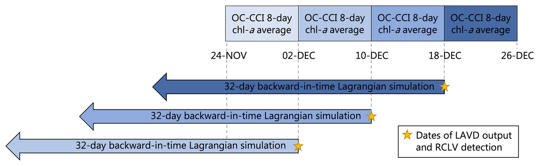
Figure B1 A schematic of the temporal alignment between 32 d backward-in-time Lagrangian trajectories, RCLV detection, and the 8 d average OC-CCI chl a observations. The blue colors match the RCLV detection dates and the collocated chl a 8 d averages.

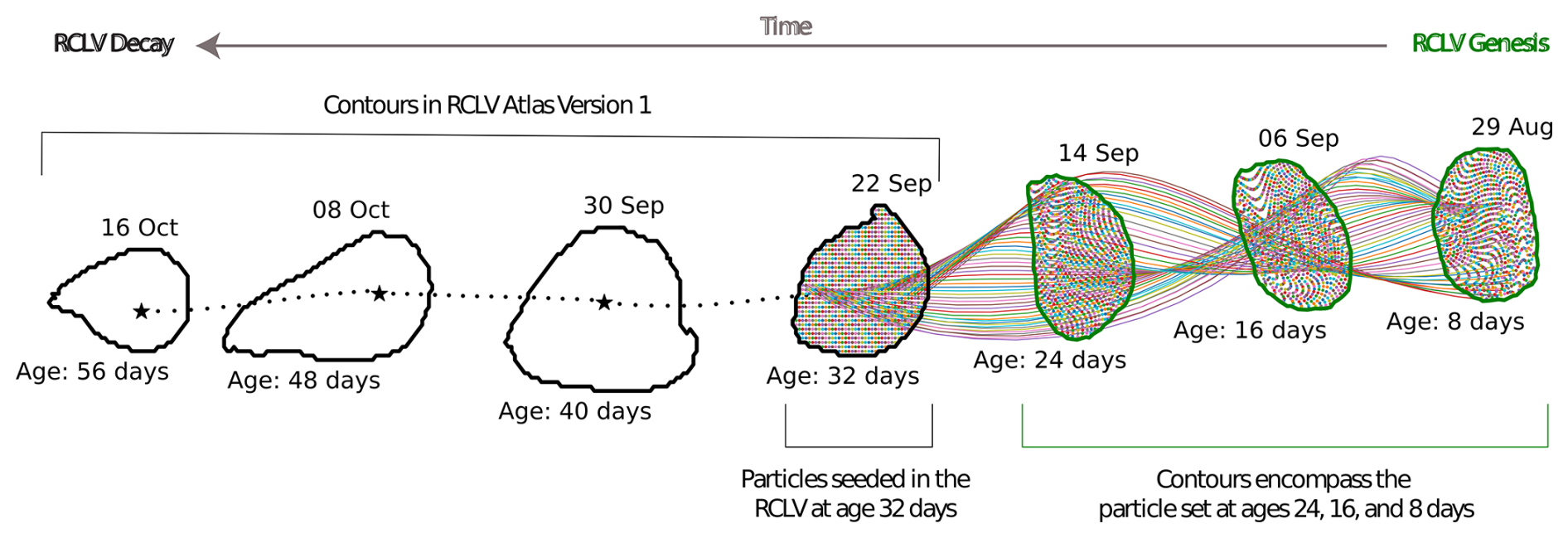
Figure B2 A schematic of the eddy genesis extension of RCLV Atlas Version 1 to 2. From Version 1, RCLVs were tracked starting at age 32 d (22 September), shown by the black contours in this example. To simulate the RCLV genesis in Version 2, we initialized Lagrangian particles (multicolored dots) in 32 d old RCLVs and tracked them backward in time (multicolored lines). The green contours drawn around the particle set are the contours included in the extended atlas, representing the RCLV boundaries at ages 24 (14 September), 16 (6 September), and 8 d (29 August).

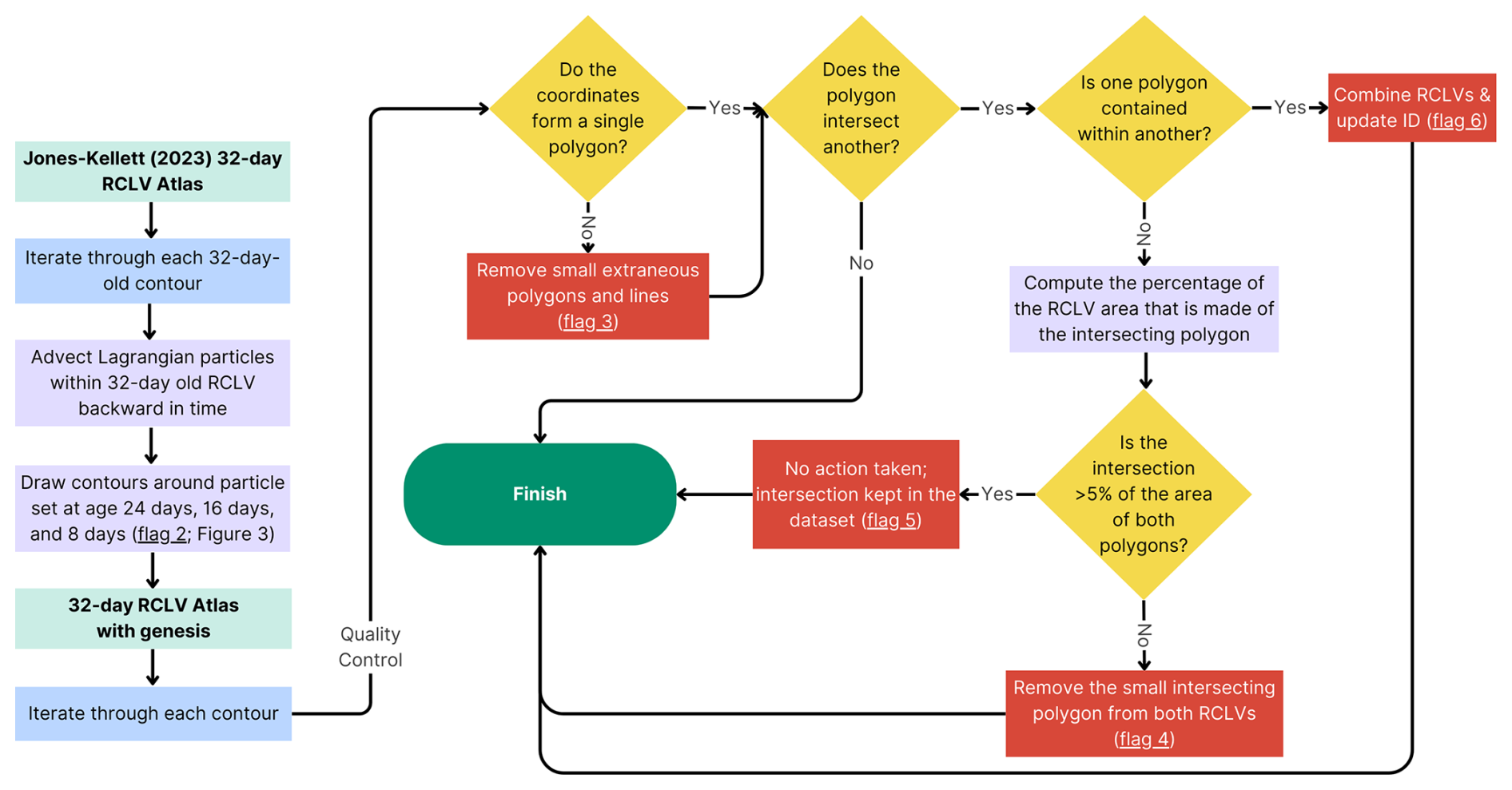
Figure B3 RCLV genesis and quality control pipeline. Particle sets were initialized in 32 d old RCLVs, and closed contours were drawn around the particles as they were advected backward-in-time. This captured the eddy genesis boundaries at ages 24, 16, and 8 d. Extraneous lines or multi-polygons were smoothed to create a single polygon (flag 3). In some rare cases, the eddy genesis contours intersected with another feature on the same day (see Table C1 for the percentage of contours). If there was a complete overlap, RCLVs were combined and assumed to be “skipped” between time steps due to noise in the SLA (flag 6). Small overlaps (<5 % of the contour areas) were removed (flag 4), and large overlaps were flagged and left unaltered (flag 5). This figure was generated with Canva software.

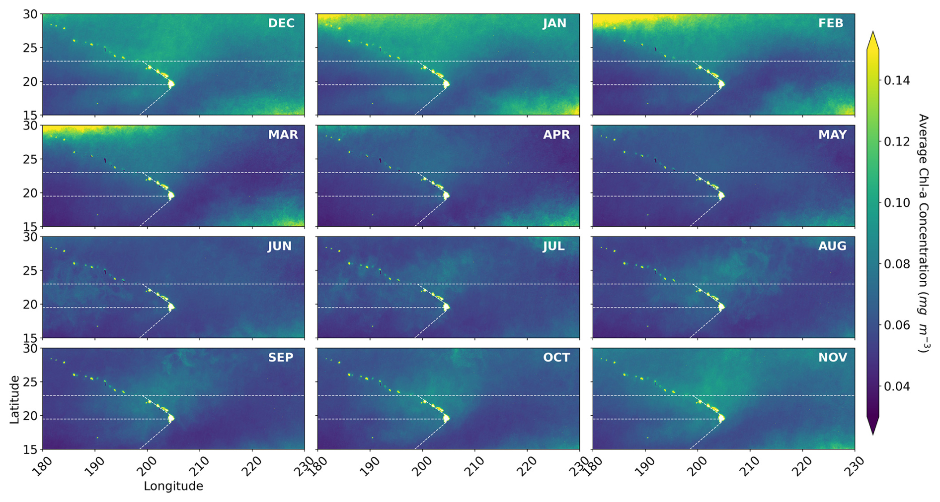
Figure B4 Monthly mean chl a derived from 2000 through 2019 OC-CCI 8 d averages. The dotted white lines delineate the regional provinces examined in this study.

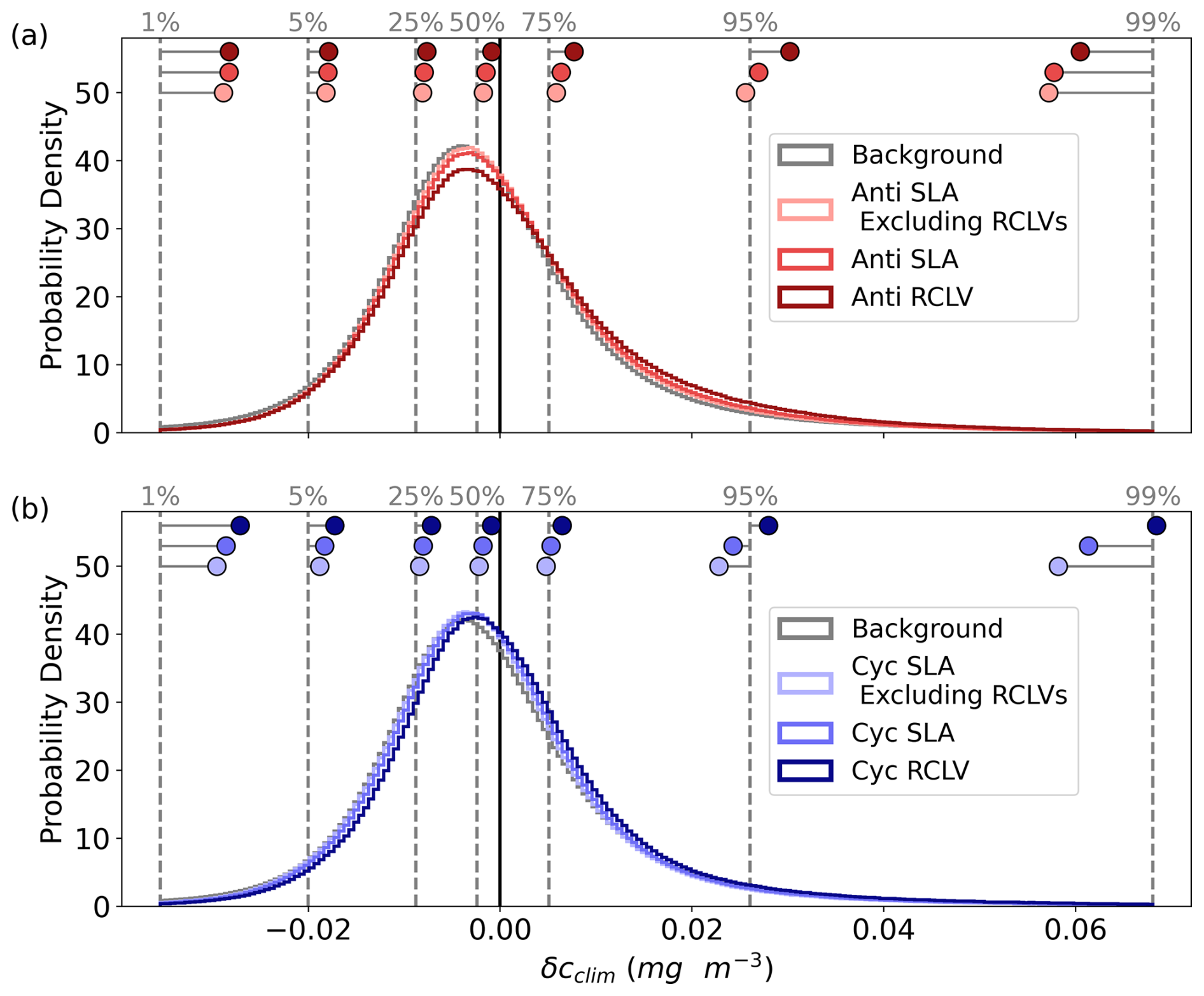
Figure B5 The probability density distributions of the climatological chl a anomalies (δc_clim; Eq. 1) for all (a) anticyclones and (b) cyclones from the 1st to 99th percentiles. The vertical, dotted gray lines depict the background distributions' percentiles (labeled with gray text). The dots show the equivalent percentiles for each eddy category, demonstrating the shifts in the distributions from the background.

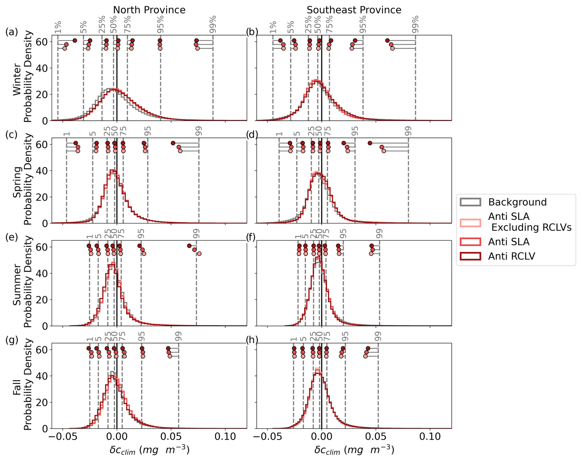
Figure B6 Probability density distributions of climatological chl a anomaly (δc_clim) for anticyclonic eddies in the north and southeast provinces. The vertical dotted gray lines depict the background distributions' percentiles (labeled with gray text) for that province and season, and the dots show the equivalent percentiles for each eddy category. The ranges shown for the histograms are from the 0.1 to 99.9 percentiles of the background δc_clim.

Figure B7 Same as Fig. B6 but for cyclonic eddies.

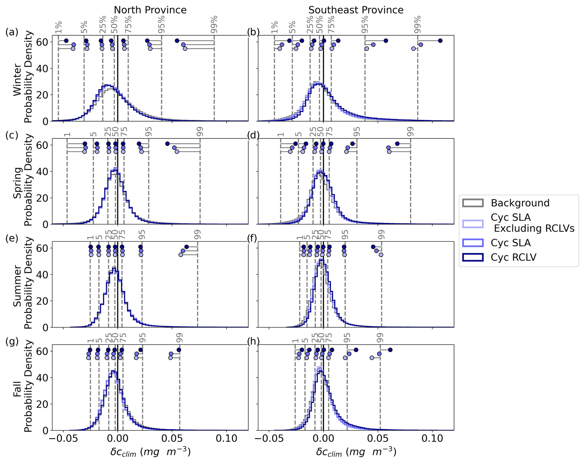
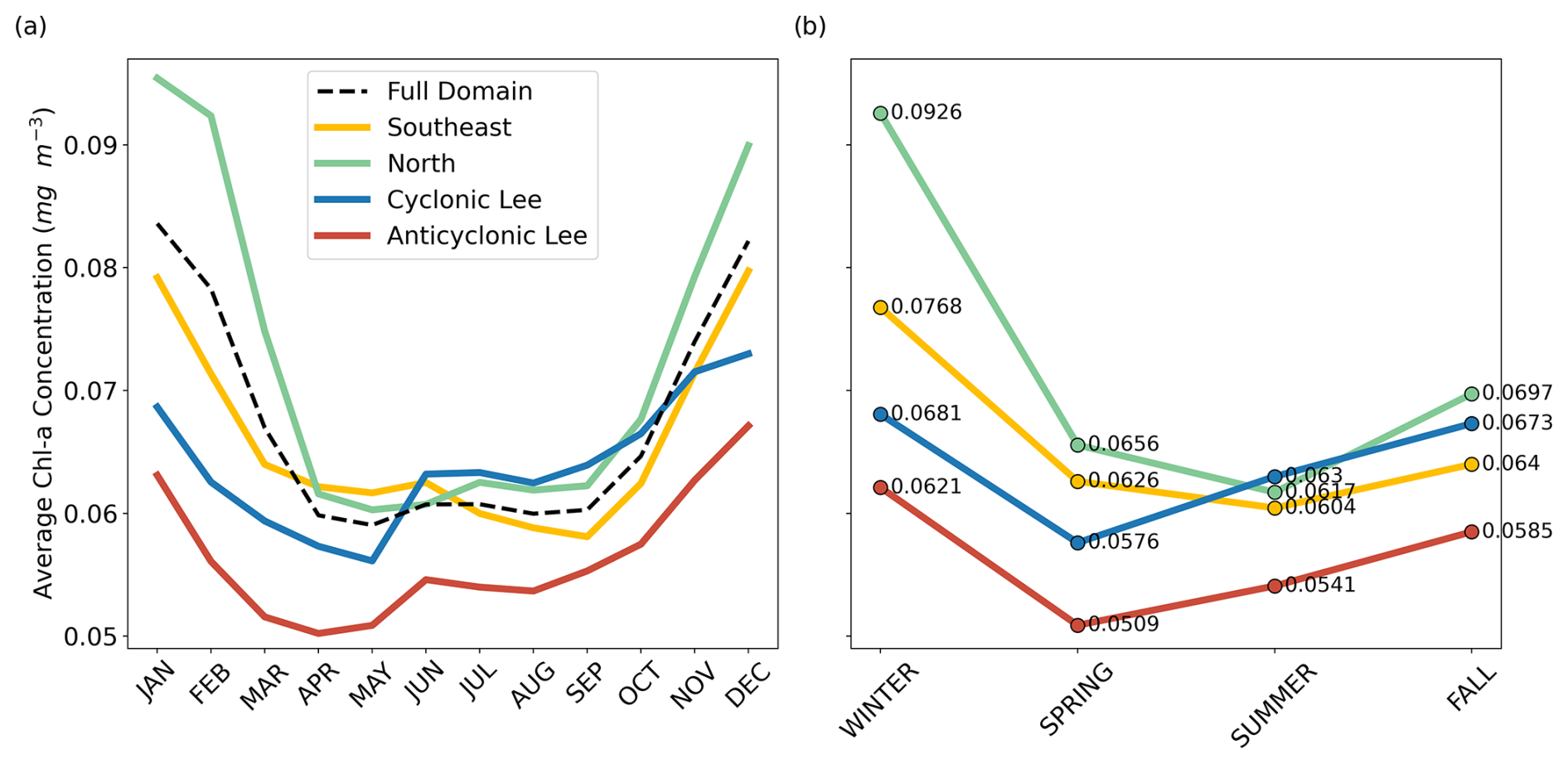
Figure B8 (a) Monthly mean chl a by province, calculated from 2000 through 2019 OC-CCI 8 d averages. The provinces correspond to the delineations made in Fig. 4a. The full domain average is closer to the north and southeast signatures because they cover the largest surface area. (b) Seasonal mean chl a by province. The numerical values of the average chl a concentrations are displayed for reference.

Figure B9 Same as Figs. B6 and B7 but for the Hawaiian lee eddies.

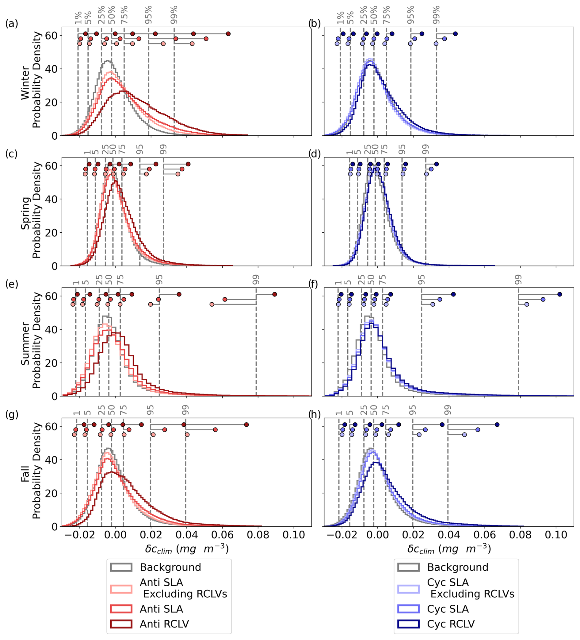
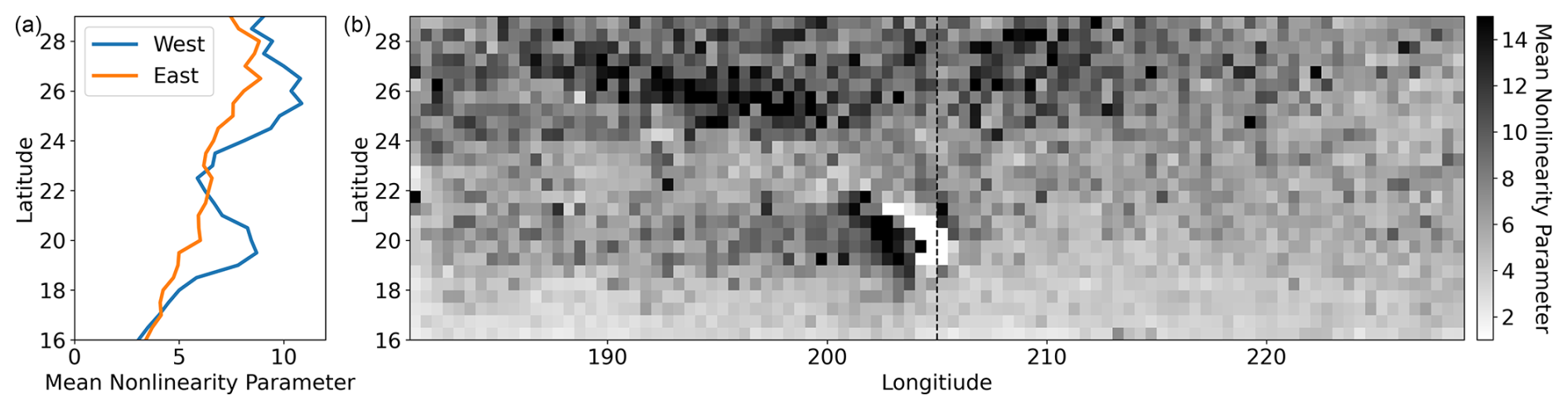
Figure B10 (a) The mean nonlinearity parameter by latitude, and (b) mapped by 1/2° grid resolution. The latitudinal averages were split by east and west at 205° E.

Appendix C: Additional tables

Table C1 RCLV Atlas Version 2 quality control flags. Note that the flags are not mutually exclusive (see Fig. B3).

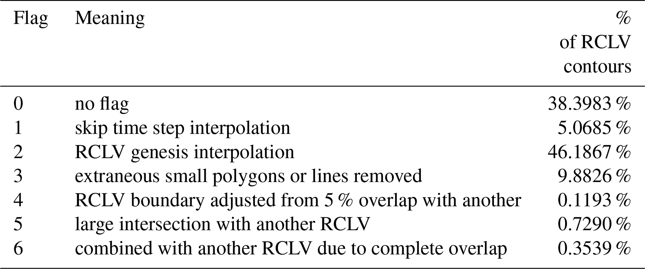
Table C2 The number of satellite Level 4 chl a pixels in each anticyclonic feature type. These counts do not include pixels where chl a is unknown due to cloud coverage or bad quality control scores.

Table C3 Same as Table C2 but for cyclonic features.

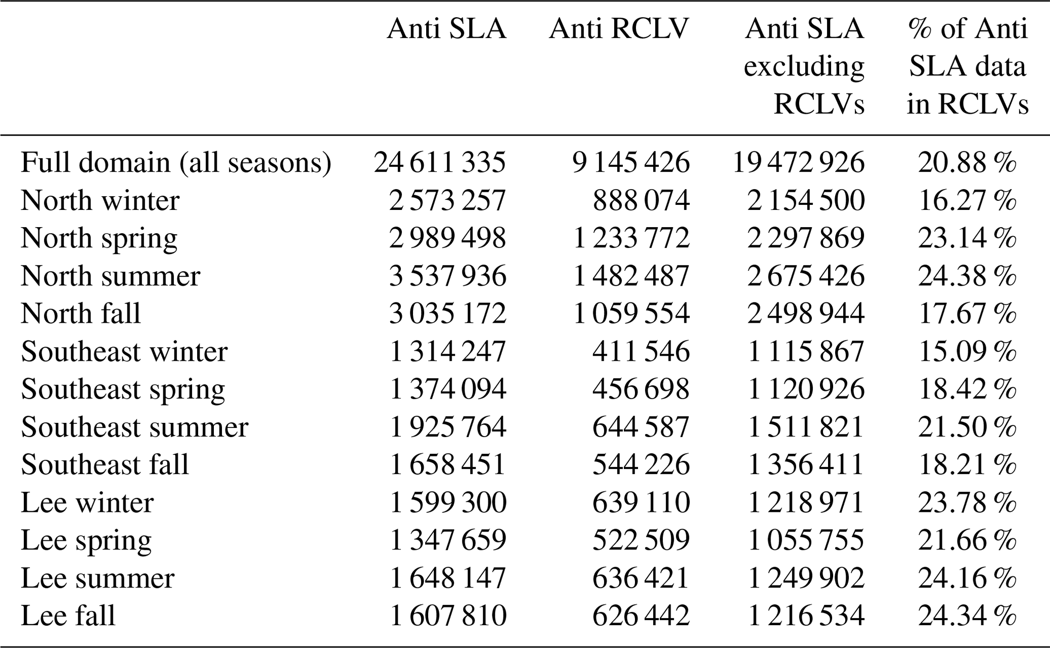
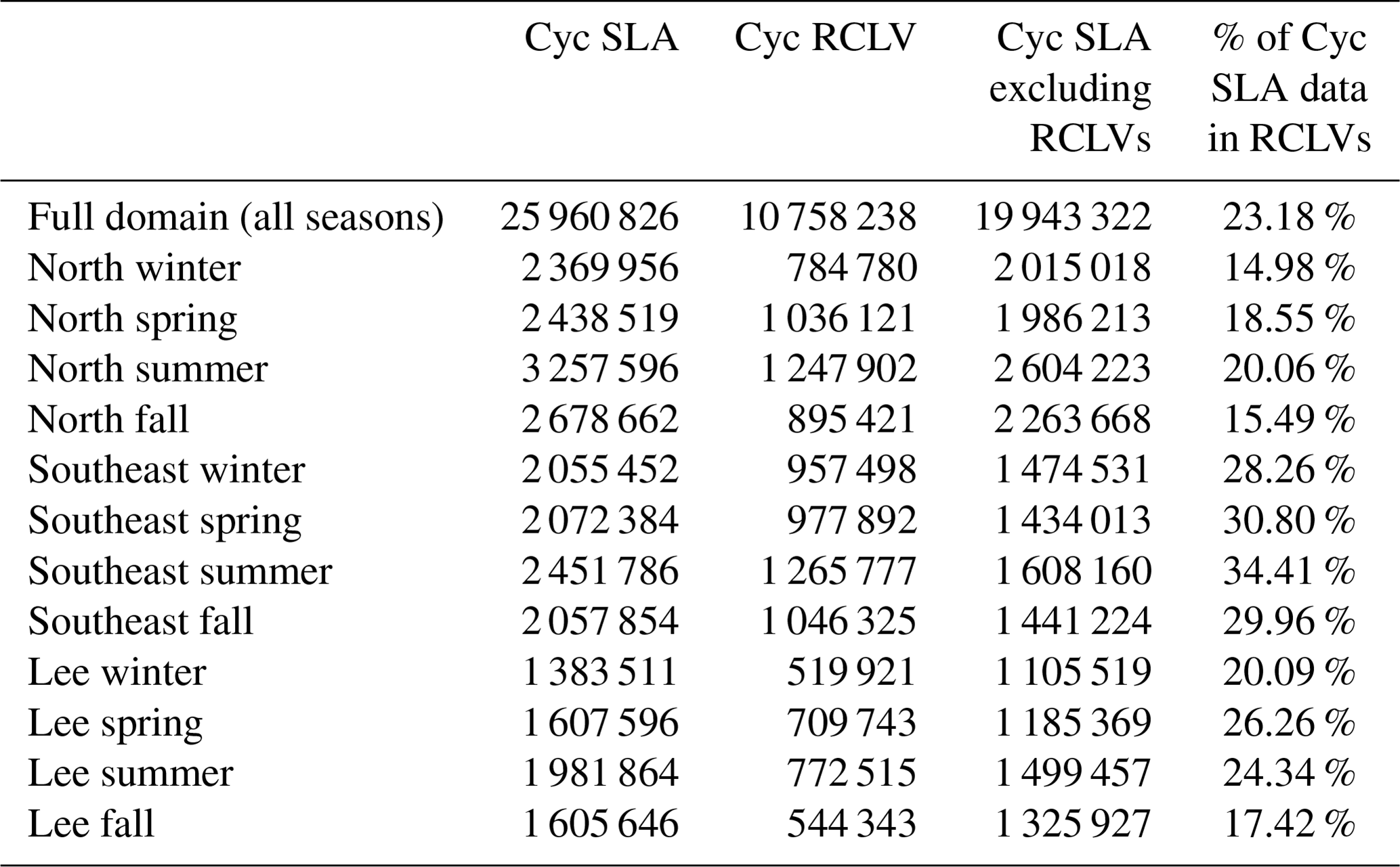
Table C4 The number of satellite Level 4 chl a pixels in the background ocean (non-eddying) and in total (background + eddy). These counts do not include pixels where chl a is unknown due to cloud coverage or bad quality control scores.