Long-term prediction of the Gulf Stream meander using OceanNet: a principled neural-operator-based digital twin

Many meteorological and oceanographic processes throughout the eastern US and western Atlantic Ocean, such as storm tracks and shelf water transport, are influenced by the position and warm sea surface temperature of the Gulf Stream (GS) – the region's western boundary current. Due to highly nonlinear processes associated with the GS, predicting its meanders and frontal position has been a long-standing challenge within the numerical modeling community. Although the weather and climate modeling communities have begun to turn to data-driven machine learning frameworks to overcome analogous challenges, there has been less exploration of such models in oceanography. Using a new dataset from a high-resolution data-assimilative ocean reanalysis (1993–2022) for the northwestern Atlantic Ocean, OceanNet (a neural-operator-based digital twin for regional oceans) was trained to predict the GS's frontal position over subseasonal to seasonal timescales. Here, we present the architecture of OceanNet and the advantages it holds over other machine learning frameworks explored during development. We also demonstrate that predictions of the GS meander are physically reasonable over at least a 60 d period and remain stable for longer. OceanNet can generate a 120 d forecast of the GS meander within seconds, offering significant computational efficiency.

1 Introduction

1.1 Background: the Gulf Stream meander

The Gulf Stream (GS) is part of the western boundary current of the Atlantic Ocean. Easily identifiable by the sea surface height (SSH) contours (Fig. 1), the GS carries warm equatorial water northward to the middle to high latitudes. The GS can be divided into two frequently studied segments: the Loop Current, which flows into and out of the Gulf of Mexico, and the Gulf Stream meander (GSM), which extends to the east once the GS passes Cape Hatteras, North Carolina (Fig. 1). Due to its vast spatial coverage and anomalously warm temperatures, the GS influences much of the weather along the eastern coast of the US, as well as western Europe (Minobe et al., 2008). Given its importance, there has been significant effort among modelers to forecast the position of the GS across various timescales.

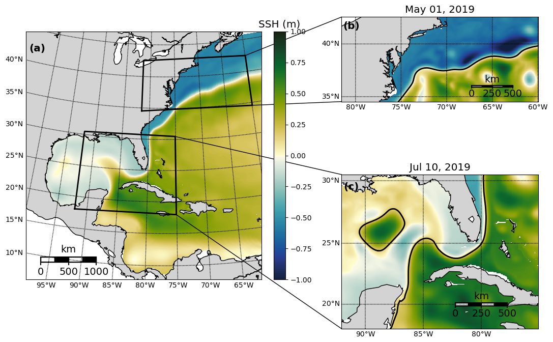
Figure 1 (a) The domain for the reanalysis data covering the northwestern Atlantic. The two subdomains used to develop OceanNet, specifically (b) the GS separation point and the GSM from the central US east coast to 60° W and (c) the Loop Current eddy-shedding region in the eastern Gulf of Mexico, extending from 92° W into the Atlantic at 75° W (not explored in this study). The mean SSH from 1993 to 2020 in the reanalysis data is shown in panel (a), while panels (b) and (c) depict the daily mean SSH on 1 May 2019 and 10 July 2019, respectively. All three domains share the same color scale.

Robinson et al. (1988) attempted to model a 26 d period of the “[GSM] and Ring region” using feature modeling techniques derived from remote-sensing data and the Harvard quasi-geostrophic open boundary model. The authors carried out multiple experiments across durations; GSM positions; and combinations of sea surface temperature, topography, and boundary conditions that were present. The following features were determined to be imperative to correctly simulate and achieve a convincing GSM and ring region: ring (eddy) formation via GSM break-offs; ring coalescence with the GSM; and ring–ring mergers, interactions, and contacts. Chen et al. (2014) modeled a case study of one particular eddy: a warm-core eddy event that lasted 27 d, detached and reattached the to GSM, and resulted in heat and salinity fluxes on the order of 6–9 times larger than mean values. Although the authors do mention that this was likely the largest and most energetic event in decades, visual inspection of sea surface variable plots (temperature, height, currents, etc.) demonstrates how mesoscale-eddy structures are frequently present around the GSM. These structures, as seen in Chen et al. (2014), can greatly influence the overall circulation and fluxes of state variables.

It has been a challenging task for numerical models to robustly simulate and predict GS dynamics, especially its separation point off Cape Hatteras, North Carolina, as well as mesoscale activity along the GSM (Chassignet and Marshall, 2008). A horizontal resolution of at least $\mathrm{1}/\mathrm{10}$° is necessary to achieve a realistic separation point (Chassignet and Marshall, 2008). Higher resolutions are needed to adequately represent the variability in the GSM, including GS meanders and eddies, and the zonal penetration of the GS (Chassignet and Xu, 2017). As GSM simulations are the result of interactions on relatively small scales that propagate to much larger processes, numerical models must be carefully calibrated and include high-resolution physics. The open boundary to the east of the GS exacerbates these challenges by requiring larger domains to properly capture meridional fluxes into the system. These compounding factors result in the need for massive compute power, time, and funding for numerical modelers. Conversely, machine learning predictions require a fraction of the resources; while these models may be slow to train, taking hours or even days, they result in extremely fast, cheap models that can exponentially reduce compute times and cost without making sacrifices in terms of resolution.

1.2 Machine learning in marine sciences

In the weather and climate modeling communities, data-driven machine learning methods have become a popular field of exploration and have delivered promising results in the prediction of complex atmospheric circulation (Kurth et al., 2023; Bi et al., 2023; Lam et al., 2023). Such models have demonstrated the aforementioned advantages of machine learning while also outperforming state-of-the-art numerical weather models for lead times of 8–10 d (Kurth et al., 2023; Bi et al., 2023; Lam et al., 2023). A significant limitation of these models arises when they are integrated over longer timescales (2 weeks or longer), leading to instability and the emergence of nonphysical features (see Chattopadhyay and Hassanzadeh, 2023, their Fig. 1). The cause of this instability was identified as “spectral bias”, an inductive bias in all deep neural networks that hinders their ability to capture small-scale features in turbulent flows. Chattopadhyay and Hassanzadeh (2023) proposed a potential solution in the form of a framework to construct long-term stable digital twins for atmospheric dynamics. That is not to say numerical weather models have a prediction horizon much longer (if at all) than 2 weeks, but the fact that machine learning atmospheric models are as accurate as they are on a global scale for any lead time – even if they grow unstable – is a tremendous feat. While these advances are proving fruitful for the atmospheric sciences, there has yet to be progress of equivalent magnitude in predicting physical systems in marine sciences.

Efforts to emulate ocean dynamics with deep-learning-based approaches have primarily focused on predicting large-scale circulation features, such as those resolved by empirical orthogonal functions (EOFs), or on constructing low-dimensional representations (Wang et al., 2019; Agarwal et al., 2021). Zeng et al. (2015) demonstrated the ability to predict SSH fields in the Gulf of Mexico associated with the Loop Current with about a 4-week lead time (up to 6 weeks in some cases) based on principle component time series of satellite-observed SSH fields. Zeng et al. (2015) later became the basis of Wang et al. (2019), where, after decomposing SSH fields in the Gulf of Mexico into principle component time series, the authors used a recurrent neural network, the long short-term memory (LSTM) model, to make a temporally informed prediction. This method achieved valuable results, showing improved prediction accuracy of SSH fields in the Gulf of Mexico for up to 12 weeks compared to persistence, which was used as the baseline. While Zeng et al. (2015) and Wang et al. (2019) are both impressive, they share a similar problem of neglecting small-scale interactions that are important to the propagation of larger-scale features, such as the separation of a Loop Current eddy from the Loop Current. These studies are certainly a step in the right direction, but there is ample need for more data-driven ocean models (e.g., Wang et al., 2024, similar to the data-driven global weather models seen in Kurth et al., 2023; Bi et al., 2023; and Lam et al., 2023).

In an attempt to advance the progress of machine learning in marine sciences, examined here is the development and performance of a neural-operator-based digital twin for the northwestern Atlantic Ocean's western boundary current, named OceanNet, built upon the same principles as the FouRKS model introduced in Chattopadhyay and Hassanzadeh (2023). OceanNet relies on a Fourier neural operator (FNO), which incorporates a predict–evaluate–correct (PEC) integration scheme to suppress autoregressive error growth. Additionally, a spectral regularizer is employed to mitigate spectral bias at small scales. OceanNet is trained on historical SSH data from a high-resolution northwestern Atlantic Ocean reanalysis and demonstrates remarkable stability and competitive skills. OceanNet, on average, outperforms SSH predictions made by the state-of-the-art Regional Ocean Modeling System (ROMS) across a 120 d period while also maintaining a computational cost that is 4 000 000× cheaper (ROMS: 10 h across 144 CPUs; OceanNet: 1.18 s on a single NVIDIA A100 GPU) following a training period of approximately 12 h (on an NVIDIA A100 GPU with 40 GB of memory).

This paper focuses on comparing variations in OceanNet and the arrival at the best architecture. For an in-depth discussion of the physical and mathematical theory behind OceanNet and each of its components, see Chattopadhyay et al. (2024).

2 Data and methods

2.1 Northwestern Atlantic Ocean reanalysis

A high-resolution northwestern Atlantic regional ocean reanalysis dataset was utilized to train OceanNet (Fig. 1) (He et al., 2025). This reanalysis was generated using ROMS with the ensemble Kalman filter data assimilation method (EnKFDA). Unlike the 4D-Var method, the EnKFDA method does not rely on future time step observations or require forward and adjoint model iterations during data assimilation. This approach enables the efficient creation of a data-assimilative ocean reanalysis, allowing OceanNet to be trained on a time–space continuous reanalysis dataset. The dataset features a horizontal resolution of $\mathrm{1}/\mathrm{25}$° with 50 vertical layers. For surface atmospheric forcing, data from the European Center for Medium-Range Weather Forecasts (ECMWF) Reanalysis v5 (ERA5) was employed, while open boundary conditions were derived from the Copernicus Global Ocean Physics Reanalysis (GLORYS). A total of 10 major tidal constituents from the Oregon State University TPXO tide database were used. The model incorporated 120 river inputs, sourced from the National Water Model and climatological datasets. The temporal scope of the reanalysis data used spans from 1 January 1993 to 31 December 2020, with daily averaged output. The assimilated observations encompass a variety of sources, including AVHRR and MODIS Terra sea surface temperature; AVISO along-track sea surface height anomaly; glider temperature and salinity observations from the Integrated Ocean Observing System (IOOS); and the EN4 dataset, which aggregates data from Argo floats, shipboard surveys, drifters, moorings, and other sources.

2.2 Model development

A summary of the model configurations discussed in the following sections can be found in Table 1 in Sect. 3.

Table 1 Summary of experiments conducted. SR refers to “spectral regularization”, “MHD saturation” refers to the number of days it takes for the saturation value to be reached, and “CC=0” denotes the amount of time it takes the respective model to have a correlation coefficient value of zero. Metrics are explained in further detail below.

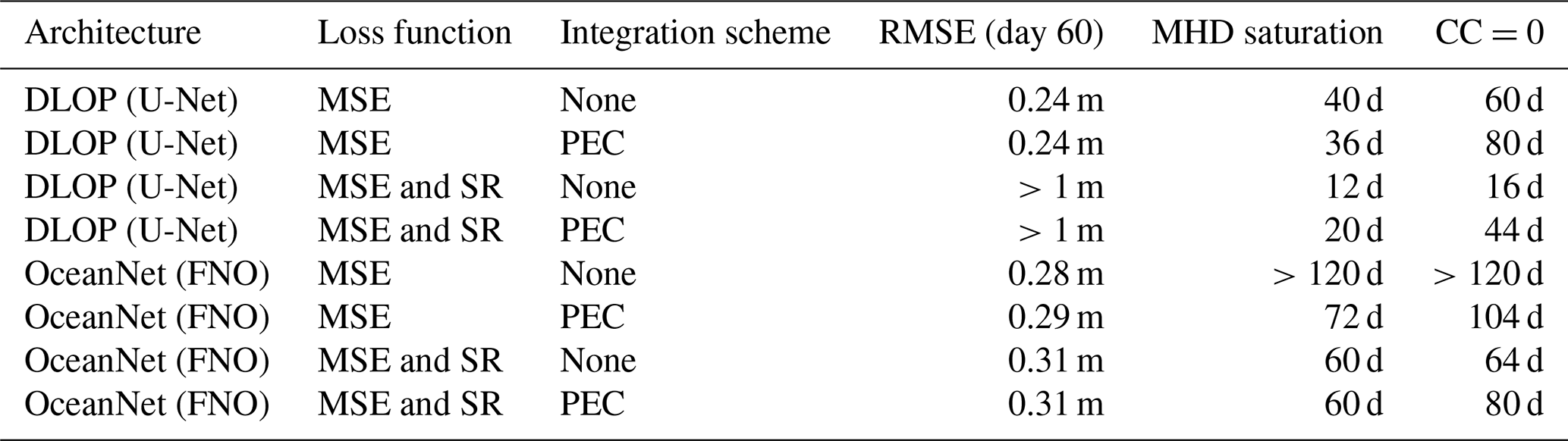
Previously undefined abbreviations used in the table are as follows: RMSE – root-mean-square error; MHD – modified Hausdorff distance; MSE – mean-squared error loss.

2.2.1 Deep learning ocean prediction

One of the ground-breaking machine learning models for weather prediction was introduced by Weyn et al. (2019): the Deep Learning Weather Prediction (DLWP) model. According to Weyn et al. (2019), DLWP has the ability to predict 500 hPa geopotential height at forecast lead times of up to 3 d and can “…easily outperform persistence, climatology, and the dynamics-based isotropic vorticity model, but not beat an operational full-physics weather prediction model”. Furthermore, Weyn et al. (2019) showed that their DLWP model can output realistic atmospheric states for up to 14 d. The capabilities of DLWP made it an attractive starting point for modeling the SSH field in regional ocean; thus, it became the first iteration of OceanNet – henceforth referred as the Deep Learning Ocean Prediction (DLOP) model.

DLOP is a relatively simple U-Net that is generally less complicated than DLWP, although the core idea is the same: pixel-wise connections of 2D fields of physical variables between time steps are sufficient to predict the evolution of such fields through time. The training of DLOP consisted of passing randomly shuffled 2D SSH images from the reanalysis dataset from the years 1993 through 2018 with a simple constraint of mean-squared error of the predicted 2D SSH field. Due to the slower evolution of ocean states than that of the 500 hPa fields used in DLWP, a lead time of 4 d was used for training. The SSH fields were resampled to 5 d running-mean fields to remove the high-frequency noise associated with the SSH, such as tidal variations. If X(t) is the initial 5 d mean field of SSH at time step t, then $X(t+\mathrm{\Delta }t)=\text{DLOP}\left(X\right(t\left)\right)$, where Δt was determined during training to be 4 d. The specifics of training of DLOP are almost identical to the final training of OceanNet – explained more thoroughly in Sect. 2.4.

Once trained, DLOP was used to autoregressively predict SSH fields out to 120 d. Initially, predictions from DLOP appeared to show quite good performance – root-mean-square error (RMSE) and correlation coefficient (CC) values for a 4 d or 8 d prediction were on-par with or better than other predictive models (time series of metrics for models discussed here can be found in Sect. 3); however, predictions using DLOP tended to a mean state within a couple of time steps before eventually growing completely unstable and, thus, nonphysical (Fig. 2). A thorough investigation of DLOP led to a similar conclusion to that of Chattopadhyay and Hassanzadeh (2023): the shortcomings of the DLOP's U-Net backbone reside in its inability to capture small-scale features in turbulent flows, as evident from the mismatch of high wavenumbers present in the fields.

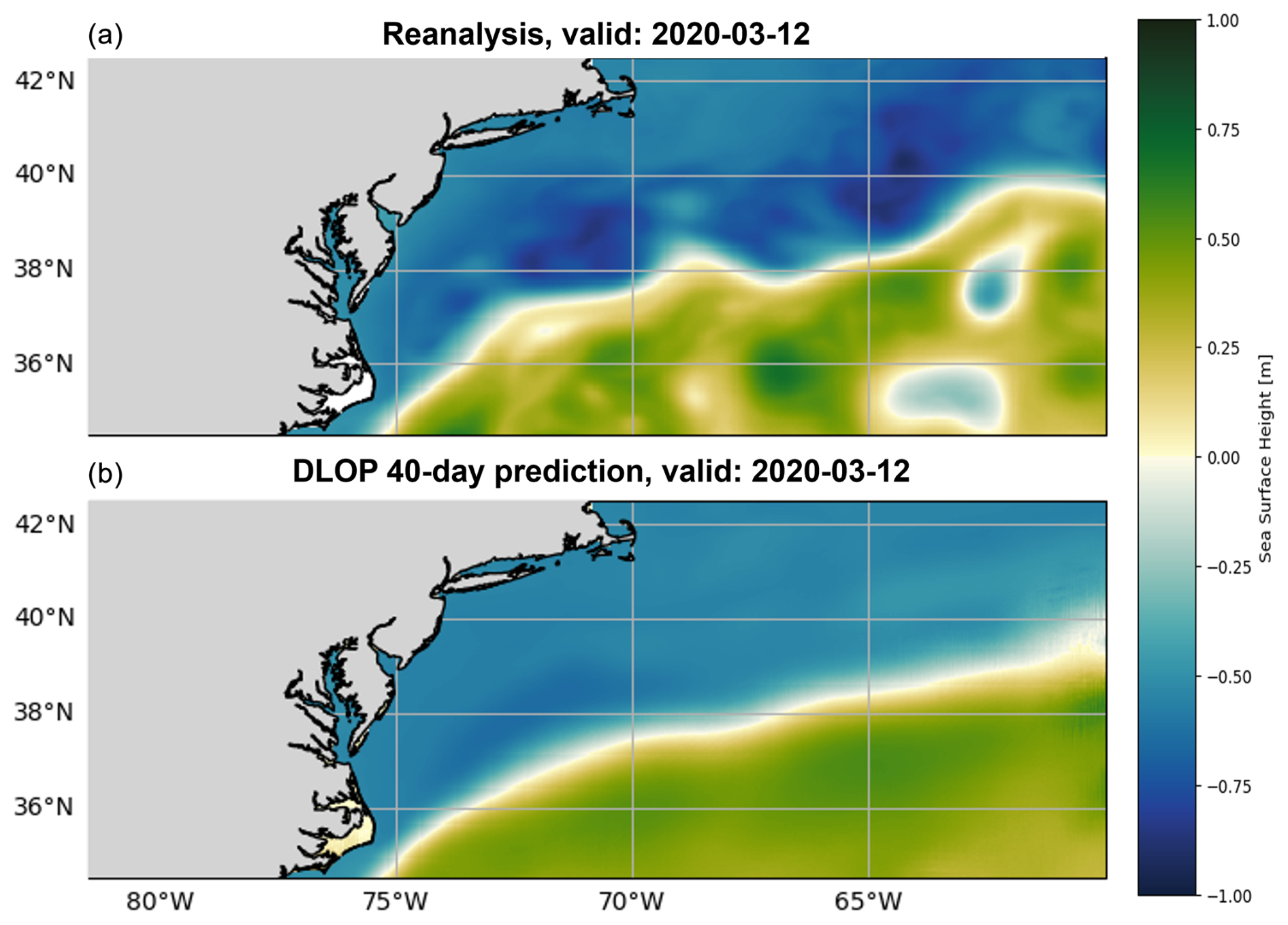
Figure 2 Predictive performance of DLOP on the GSM region at 40 d. Panel (a) presents the SSH field from the reanalysis dataset 40 d after DLOP's initialization. Panel (b) corresponds to the SSH field of DLOP's 40th day of prediction, demonstrating the model tending to the background state of the GSM.

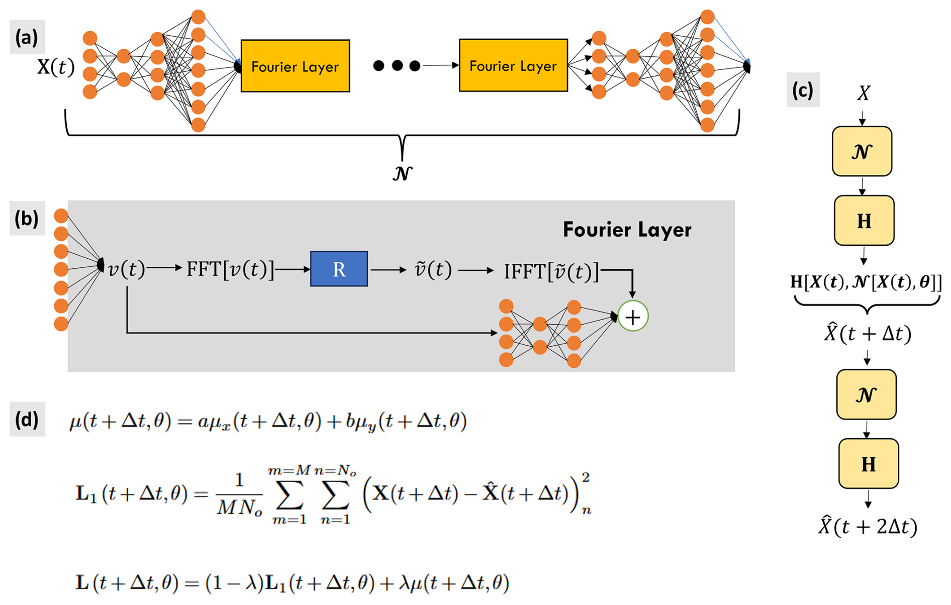
Figure 3 A schematic of the OceanNet model with input image X(t). Panel (a) presents the Fourier neural operator, 𝒩. Prior to entering the Fourier layers, the input image is fed through a multilayer perceptron consisting of two convolutions. The output of each of the Fourier layers is activated with the Gaussian error linear unit function. Following the last Fourier layer, the data are fed through two more convolutions to preserve the dimensions of the final output. Panel (b) shows the Fourier layer. A Fourier transform is performed on ν(t), the higher-dimensional representation of the input image, followed by a linear operation, R, to reduce the highest Fourier modes to zero, resulting in $\stackrel{\mathrm{̃}}{\mathit{\nu }}\left(t\right)$. An inverse Fourier transform brings $\stackrel{\mathrm{̃}}{\mathit{\nu }}\left(t\right)$ back to its original space. The resulting tensor is then concatenated with the input to the Fourier layer, to which a 2D convolution has been applied. OceanNet contains four Fourier layers. Panel (c) presents the two-time-step scheme with the numerical integration operator, H. Panel (d) shows the point-wise loss function used, constructed by the spectral regularizer μ and MSE, L₁, for M samples and applied to all N_o ocean points. The loss function is discussed in greater detail in Sect. 2.4.1.

Efforts were made to try and combat this documented phenomenon, specifically those prescribed by Chattopadhyay and Hassanzadeh (2023) known as the FouRKS framework. The FouRKS framework consists of employing numerical integration (Sect. 2.3.2) and spectral regularization (Sect. 2.4.1) techniques to suppress autoregressive error growth and encourage the model's attention to correctly predict the smaller-scale features present. The inclusion of numerical integration in the model architecture did improve the stability horizon of the model and, thus, led to much lower metric values of the RMSE and CC over the 120 d prediction period, but an investigation into the actual images being produced by the model showed that DLOP was slowly tending to what can only be described as a background state of the GSM. While the numerical integration techniques helped to some degree, the spectrum of the model was still an inaccuracy of interest that could potentially be fixed when paired with the spectral regularizer. Unfortunately, both with and without the presence of the numerical integration scheme, the spectral regularizer caused DLOP to become even more unstable than before, as can be seen from the metrics alone – after two time steps, the model loses all physicality and immediately propagates noise throughout the domain.

The failures of DLOP quickly evolved into a complicated problem. Despite the documentation for what was being seen by Chattopadhyay and Hassanzadeh (2023), a stable and accurate U-Net for ocean prediction could not be achieved. In numerical modeling, the suppression of error can typically be handled by integrating on shorter timescales or by adding constraints to the system to discourage the development of instability. For DLOP, integrating on shorter timescales would mean predicting with a smaller lead time each time step, which was attempted. Although the results are not shown here, extensive trial and error revealed that integrating on lead times of less than 4 d led to DLOP not propagating anything forward – in other words, the evolution of the SSH field over 3 d or fewer is so small that the training process resulted in DLOP determining it would achieve the lowest error if it kept the field completely static with every prediction. This may not be a problem with atmospheric prediction, as in DLWP, because the evolution of the atmosphere is noticeable over much shorter timescales. As for constraining the system to suppress error, this was the intent of the spectral regularization techniques but no improvement was observed.

2.3 OceanNet

Given that the analysis of the DLOP results is consistent with previous literature and that there was a noticeable improvement in the stability of DLOP with the inclusion of the numerical integration scheme, the techniques seen in Chattopadhyay and Hassanzadeh (2023) continued to be employed. While the spectral regularization scheme did not provide much (if any) improvement to DLOP, the idea of constraining the system's distribution of wavenumbers and stabilizing autoregressive prediction remained attractive; however, instead of using the typical 2D convolutions with a U-Net structure, Fourier neural operators (FNOs) with a multi-time-step loss function were thought to provide similar behavior. This section provides more information regarding FNOs and numerical integration, while Sect. 2.4.1 further explains the spectral regularization and the multi-time-step constraints used in the final version of OceanNet.

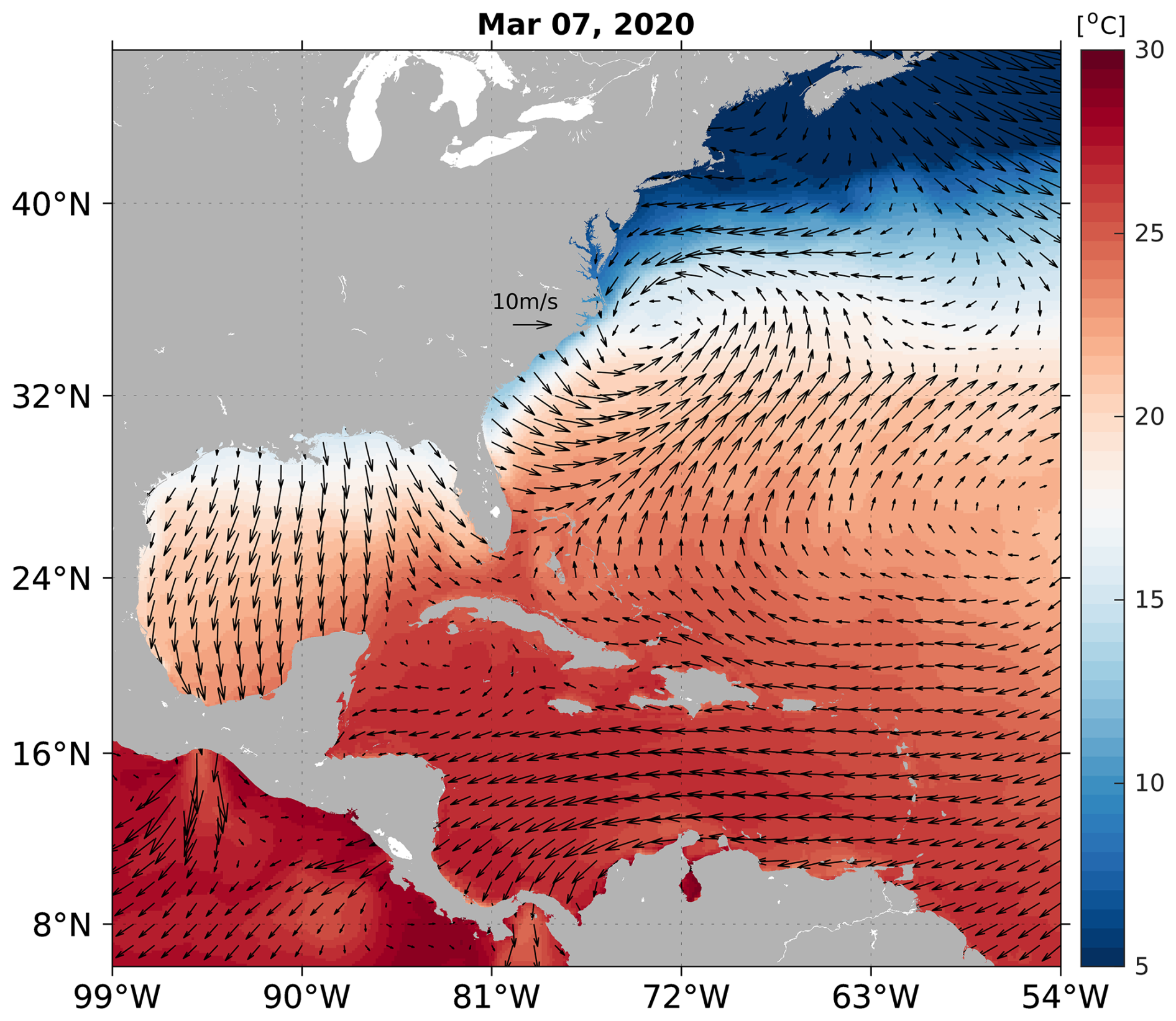
Figure 4 An example of atmospheric conditions used to force the uncoupled numerical simulations in ROMS – used in the simulation initialized on 7 March 2020. Variables shown in the figure are as follows: 2 m air temperature (shading) and 10 m wind vectors (every eighth grid point plotted for visual clarity).

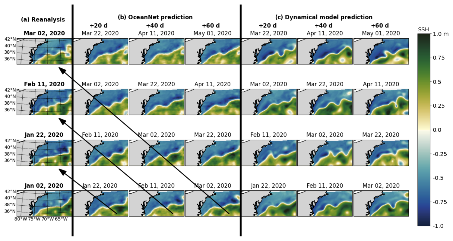
Figure 5 Performance of OceanNet for GS prediction. Panel (a) presents the SSH fields from the ocean reanalysis. Panel (b) shows the predicted SSH generated by OceanNet. Panel (c) displays the ROMS dynamical model forecasts. In both OceanNet and dynamical model predictions, each row was initialized with the corresponding reanalysis data in the left column. SSH forecasts are provided for 20, 40, and 60 d. To evaluate the predictions, we can perform a diagonal comparison with the reanalysis SSH, as indicated by the black arrows in panel (b). The same diagonal comparison can also be conducted with the ocean reanalysis data in panel (c).

2.3.1 Fourier neural operator (FNO)

OceanNet is built upon the FNO. FNOs were introduced in Li et al. (2020), where the authors demonstrate higher performance benchmarks in terms of speed and error than any other deep learning technique to date when modeling complex fluid flow problems such as Burgers' equation, Darcy flow, and the Navier–Stokes equations. Due to performing operations in Fourier space, the FNO is considered to be resolution-agnostic; this is an advancement in and of itself because prior methods of deep learning for image-to-image translation required the consistent use of the training data's resolution. The speed of FNOs comes from the various advancements in the computer science fields which have led to extremely efficient implementations of the fast Fourier transform. Furthermore, FNOs do not rely on scanning the information in 2D space as convolution and pooling layers do; instead, they integrate the whole field at once. Our implementation of the FNO, denoted by 𝒩, begins with the input field X(t) being fed through a multilayer perceptron consisting of two convolution layers before passing to the Fourier layers. Following the methods of Li et al. (2020), a Fourier layer takes a high-dimensional representation of the input field, applies a Fourier transform, reduces the highest Fourier modes to zero, and applies an inverse Fourier transform to bring the data back to their original space (Fig. 3b). The resulting tensor is then concatenated with the input to the Fourier layer, to which a 2D convolution has been applied to account for aperiodicity in the data (Fig. 3b). OceanNet includes four Fourier layers, with Gaussian error linear unit activations following each layer.

As with DLOP, training utilizes labeled pairs of historical 5 d running-mean SSH data in the GSM, X(t) (image), X(t+Δt) (label), and X(t+2Δt) (label), where Δt=4 d. The training assumes that the governing partial differential equation for the reduced ocean system involves ocean states X(t):

$$\begin{array}{}\text{(1)}& {\displaystyle }{\displaystyle \frac{\mathrm{d}\mathbf{X}}{\mathrm{d}t}}=\mathbf{F}\left(\mathbf{X}\left(t\right)\right).\end{array}$$

To integrate the system from the initial condition, X(t), Eq. (1) is represented in its discrete form:

$$\begin{array}{}\text{(2)}& {\displaystyle }{\displaystyle }\widehat{\mathbf{X}}(t+\mathrm{\Delta }t)=\underset{\mathbf{H}[\circ ]}{\underbrace{\mathbf{X}\left(t\right)+\underset{t}{\overset{t+\mathrm{\Delta }t}{\int }}\underset{\mathcal{N}[\circ ,\mathit{\theta }]}{\underbrace{\mathbf{F}\left(\mathbf{X}\left(t\right)\right)}}\mathrm{d}t}}.\end{array}$$

Here, $\widehat{\mathbf{X}}(t+\mathrm{\Delta }t)$ is the new SSH field resulting from a single predictive step. $\mathcal{N}[\circ ,\mathit{\theta }]$ is the neural network which will parameterize F with four Fourier layers, similar to Li et al. (2020), with each layer retaining 64 Fourier modes. θ represents the $\approx \mathrm{80}\times {\mathrm{10}}^{\mathrm{6}}$ trainable parameters of the FNO. H[∘] represents an operator encompassing the numerical technique used to evaluate the right-hand side of Eq. (2) and will henceforth be referred to as the “numerical integration scheme”; e.g.,  the final version of OceanNet uses a higher-order predictor–evaluate–corrector (PEC) integration scheme (Sect. 2.3.2).

$$\begin{array}{}\text{(3)}& {\displaystyle }{\displaystyle }⟹\widehat{\mathbf{X}}(t+\mathrm{\Delta }t)=\mathbf{H}\left[\mathbf{X}\right(t),\mathcal{N}[\mathbf{X}\left(t\right),\mathit{\theta }\left]\right]\end{array}$$

In practical terms, the increment Δt is predicted by feeding the initial image X(t) into our neural network 𝒩 with parameters θ. The numerical integration scheme H is then applied to the outputs, as discussed in Chattopadhyay and Hassanzadeh (2023), to give the future time step X(t+Δt).

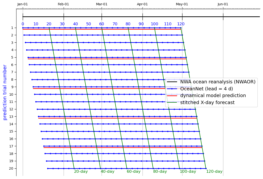
Figure 6 OceanNet's performance metrics in the northwestern Atlantic – RMSE (top), CC (middle), and MHD (bottom) – compared to the persistence forecast and ROMS dynamical model forecast. The performance statistics, calculated based on forecasts of 0–120 d, are displayed as mean values (lines) with their standard deviations (shading). The horizontal dashed black lines denote saturation values, which are determined as 95 % of the means derived from 1000 pairs of random images in the reanalysis dataset. These representations illustrate how each method's statistics compare with the target SSH from the reanalysis dataset.

2.3.2 Predict–evaluate–correct (PEC) integration scheme

Similar to the higher-order integration scheme in the form of fourth-order Runge–Kutta (RK4) used in Chattopadhyay and Hassanzadeh (2023), the PEC scheme is implemented in OceanNet, represented by the operator, H[∘]. The operations in H[∘] are given by the following:

$$\begin{array}{ll}\text{(4a)}& {\displaystyle }& {\displaystyle }{\mathcal{N}}_{\mathrm{1}}=\mathcal{N}\left[\mathbf{X}\left(t\right),\mathit{\theta }\right],{\displaystyle }& {\displaystyle }\widehat{\mathbf{X}}(t+\mathrm{\Delta }t)=\mathbf{H}\left[\mathbf{X}\right(t),\mathcal{N}[\mathbf{X}\left(t\right),\mathit{\theta }\left]\right]\\ \text{(4b)}& {\displaystyle }& {\displaystyle }=\mathbf{X}\left(t\right)+\mathcal{N}\left[\mathbf{X}\left(t\right)+{\displaystyle \frac{\mathrm{1}}{\mathrm{2}}}{\mathcal{N}}_{\mathrm{1}},\mathit{\theta }\right],\end{array}$$

where 𝒩₁ represents the operations of the neural network, prior to being numerically integrated. The final predicted state is given by $\mathbf{H}\left[\mathbf{X}\right(t),\mathcal{N}[\mathbf{X}\left(t\right),\mathit{\theta }\left]\right]$. Recall that 𝒩 is our neural network and H[∘] is the operator performing the numerical integration.

Although most of the higher-order integration schemes, including RK4, demonstrate good performance for this problem, PEC has been identified as the most effective choice due to its compromise between higher-order integration and memory consumption during training. A theoretical study of the effect of each integration scheme on the inductive bias of the trained N is an active area of research, especially for understanding the role that it plays on the subsequent spectral bias (Krishnapriyan et al., 2023).

As mentioned above, H[∘] may be chosen as any numerical integration scheme. For example, if one were to choose to use the implicit Euler scheme, Eq. (4b) would become

$$\begin{array}{}\text{(5)}& {\displaystyle }{\displaystyle }\widehat{\mathbf{X}}(t+\mathrm{\Delta }t)=\mathbf{H}\left[\mathbf{X}\right(t),\mathcal{N}[\mathbf{X}\left(t\right),\mathit{\theta }\left]\right]=\mathbf{X}\left(t\right)+\mathcal{N}\left[\mathbf{X}\right(t),\mathit{\theta }].\end{array}$$

In Sect. 3, experiments are described for a variety of models, some of which did not employ a numerical integration scheme in their methods. In such cases, the integration scheme is not present during the training of the neural network, 𝒩; thus, the model is directly predicting the next time step as is commonly seen in convolutional neural network (CNN) and U-Net models, such as those discussed in Sect. 2.2.1. The equation representing such models can be given as follows:

$$\begin{array}{}\text{(6)}& {\displaystyle }{\displaystyle }\widehat{\mathbf{X}}(t+\mathrm{\Delta }t)=\mathbf{H}\left[\mathcal{N}\right[\mathbf{X}\left(t\right),\mathit{\theta }\left]\right]=\mathcal{N}\left[\mathbf{X}\right(t),\mathit{\theta }].\end{array}$$

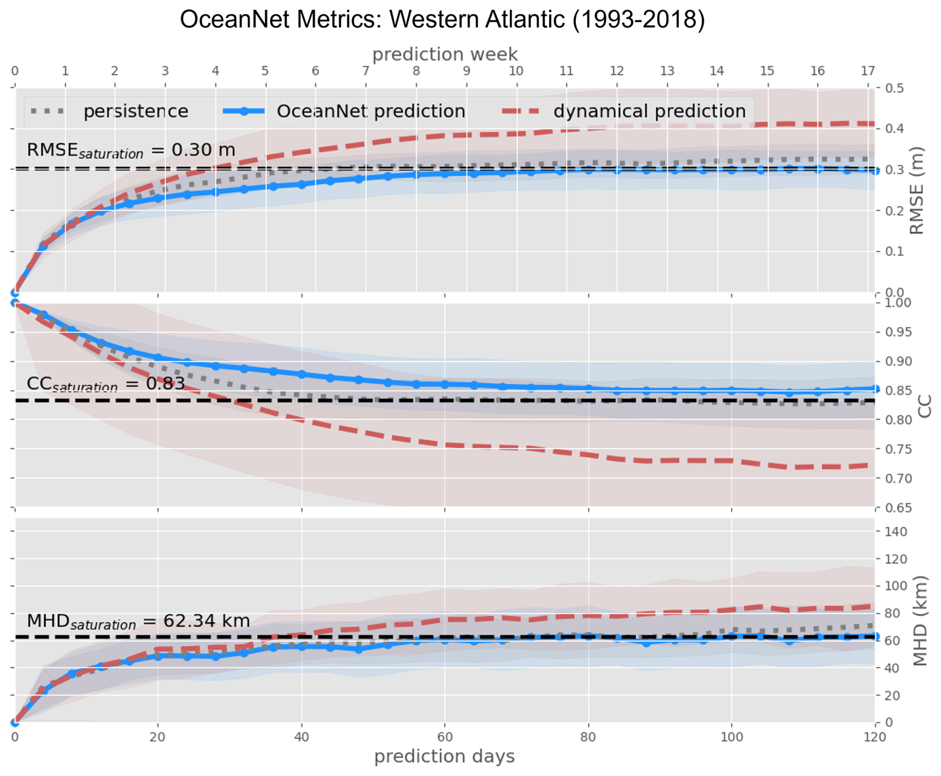
Figure 7 Visual explanation (example) of the ensembling of metrics for the evaluation of OceanNet across various ocean states. The explanation is framed with reference to OceanNet, but it applies to the analysis of all iterations of the DLOP and FNO models. The black line shows the time period covered by the reanalysis dataset with daily output. Blue lines represent individual OceanNet prediction trials spanning 120 d, each initialized 1 d apart, while blue dots indicate output time steps of the model (every 4 d). Red lines represent individual ROMS predictions, which were initialized every 5 d with output given every day. Trials where the initialization dates between both ROMS and OceanNet align were compared qualitatively (visual comparison of output fields) along the green lines and quantitatively (RMSE, CC, and MHD) at all time steps.

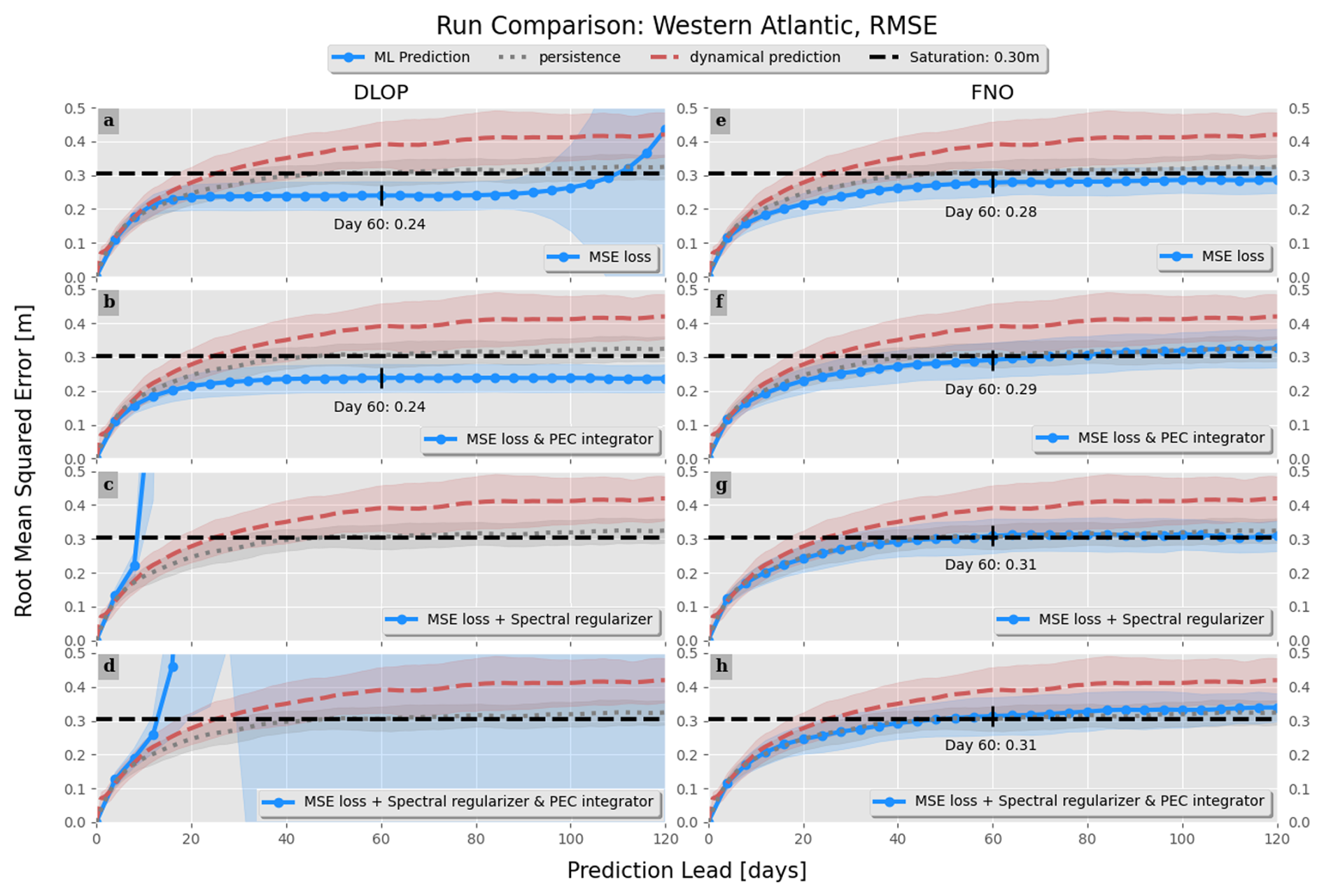
Figure 8 Comparison of the RMSE between combinations of models, integration schemes, and loss function terms. Values with an RMSE at day 60 are indicated. Line colors and styles are indicated by the legend and represent the mean value across all model runs. Shading represents the range of ±1 standard deviation. Panels (a)–(d) show the DLOP models, whereas panels (e)–(h) present the FNO models. Panels (a) and (e) are the MSE loss function with no integration scheme present, panels (b) and (f) are the MSE loss function with PEC integration, panels (c) and (g) are the MSE with spectral regularization and no integration scheme present, and panels (d) and (h) are the MSE with spectral regularization and PEC integration. Due to instabilities in the models, panels (c) and (d) had RMSE values of high enough magnitude that we are unable to show them in a meaningful plot.

2.4 Training and validation

OceanNet for the GSM was trained on 5 d running-mean SSH reanalysis fields from 1993 to 2018, which helped remove high-frequency features like tides. The years 2019 and 2020 were reserved for validation and testing. All data used for training, validation, and testing underwent the same 5 d running-mean procedure. Before training, all of the data were randomly shuffled. There are two general steps to training OceanNet: single-time-step training and multi-time-step training. Prior to either training segment, the SSH data are normalized by removing the pixel-wise 30-year mean and dividing by the pixel-wise 30-year standard deviation. After normalization, the input images are fed into the model where a 4 d lead prediction is given. For single-time-step training, the prediction and the reanalysis image of the corresponding day are evaluated by the loss function (described in Sect. 2.4.1). For multi-time-step training, the output of the model is fed back through the model to produce an 8 d lead prediction which is then evaluated by the two-time-step loss function. Based on hyperparameter optimization via the Optuna Python package, the optimal training workflow included 180 epochs of single-time-step training followed by 180 epochs of multi-time-step training. Two values were used to validate OceanNet's performance: the modified Hausdorff distance (MHD; explained in Sect. 3) and the value of the loss function.

2.4.1 Spectral regularization in Fourier space and the two-time-step loss function

In OceanNet's loss function, spectral regularization was incorporated based on Fourier transforms, introduced in Chattopadhyay and Hassanzadeh (2023). This is in addition to the standard mean-squared error loss (MSE) function, which is computed exclusively for grid points located over the ocean. The spectral regularizer penalizes deviations in the Fourier modes present in the SSH field at small wavenumbers. Such deviations arise due to spectral bias, which represents an inherent inductive bias in deep neural networks (Xu et al., 2019; Chattopadhyay and Hassanzadeh, 2023). This bias is responsible for their limitations in learning the fine-scale dynamics of turbulent flow. This regularization was carried out across both x and y dimensions to ensure that the high wavenumbers in the Fourier spectrum of the SSH remain consistent with the target Fourier spectrum.

$$\begin{array}{ll}{\displaystyle }& {\displaystyle }{\mathit{\mu }}_x(t+\mathrm{\Delta }t,\mathit{\theta })={\displaystyle \frac{\mathrm{1}}{M(K_{N_x}-K_{\mathrm{c}x})}}\\ \text{(7a)}& {\displaystyle }& {\displaystyle }\times \sum _{m=\mathrm{1}}^{m=M}\sum _{k=K_{\mathrm{c}x}}^{k=K_{N_x}}\left|{\widehat{\mathcal{F}}}_x\right[\mathbf{X}(t+\mathrm{\Delta }t)]-{\widehat{\mathcal{F}}}_x[\widehat{\mathbf{X}}(t+\mathrm{\Delta }t)]{|}_k,{\displaystyle }& {\displaystyle }{\mathit{\mu }}_y(t+\mathrm{\Delta }t,\mathit{\theta })={\displaystyle \frac{\mathrm{1}}{M(K_{N_y}-K_{\mathrm{c}y})}}\\ \text{(7b)}& {\displaystyle }& {\displaystyle }\times \sum _{m=\mathrm{1}}^{m=M}\sum _{k=K_{\mathrm{c}y}}^{k=K_{N_y}}\left|{\widehat{\mathcal{F}}}_y\right[\mathbf{X}(t+\mathrm{\Delta }t)]-{\widehat{\mathcal{F}}}_y[\widehat{\mathbf{X}}(t+\mathrm{\Delta }t)]{|}_k\end{array}$$

$$\begin{array}{}\text{(8)}& {\displaystyle }{\displaystyle }\mathit{\mu }(t+\mathrm{\Delta }t,\mathit{\theta })=a{\mathit{\mu }}_x(t+\mathrm{\Delta }t,\mathit{\theta })+b{\mathit{\mu }}_y(t+\mathrm{\Delta }t,\mathit{\theta })\end{array}$$

Here, M is the number of training samples (batch size); k represents a single Fourier mode; K_N is the highest Fourier mode present along the respective axis; K_c is the “cutoff” Fourier mode, i.e., the minimum mode of interest; and ${\widehat{\mathcal{F}}}_x$ and ${\widehat{\mathcal{F}}}_y$ denote Fourier transforms along the zonal and meridional axis, respectively. Recall that $\widehat{\mathbf{X}}\left(t\right)$ is the predicted SSH field at time t and X(t) is the SSH field given by the reanalysis at time t. After extensive trial and error, the best performance of OceanNet was observed with K_cx=10 and K_cy=30. Coefficients a and b are scaling factors used to ensure that the order of magnitude of μ_x agrees with the order of magnitude of μ_y as well as the magnitude of the MSE loss (Eq. 9a). Both a and b were determined via hyperparameter optimization to be 0.25. After combining our spectral loss function with the typical MSE loss, the full loss function for t+Δt given by $L(t+\mathrm{\Delta }t,\mathit{\theta })$ is as follows:

$$\begin{array}{ll}{\displaystyle }& {\displaystyle }{\mathbf{L}}_{\mathrm{1}}(t+\mathrm{\Delta }t,\mathit{\theta })={\displaystyle \frac{\mathrm{1}}{M{N}_{\mathrm{o}}}}\\ \text{(9a)}& {\displaystyle }& {\displaystyle }\times \sum _{m=\mathrm{1}}^{m=M}\sum _{n=\mathrm{1}}^{n=N_{\mathrm{o}}}\left(\mathbf{X}\right(t+\mathrm{\Delta }t)-\widehat{\mathbf{X}}(t+\mathrm{\Delta }t){)}_n^{\mathrm{2}},\text{(9b)}& {\displaystyle }& {\displaystyle }\mathbf{L}(t+\mathrm{\Delta }t,\mathit{\theta })=(\mathrm{1}-\mathit{\lambda }){\mathbf{L}}_{\mathrm{1}}(t+\mathrm{\Delta }t,\mathit{\theta })+\mathit{\lambda }\mathit{\mu }(t+\mathrm{\Delta }t,\mathit{\theta }),\end{array}$$

where L₁ is the MSE over N_o ocean grid points and λ is a weighting factor determined via hyperparameter optimization to be 0.2. During single-time-step training, a weighted loss function of spectral regularization and MSE is used to constrain the model. To stabilize the model over multiple autoregressive predictions, the loss function is generalized to incorporate the sum of the loss function evaluated at each predictive step. The number of time steps over which the loss is calculated can be extended to any number of autoregressive steps. However, with each increase in the number of time steps the memory requirement for the subsequent backpropagation process during training grows exponentially; thus, the compromise of two time steps was reached.

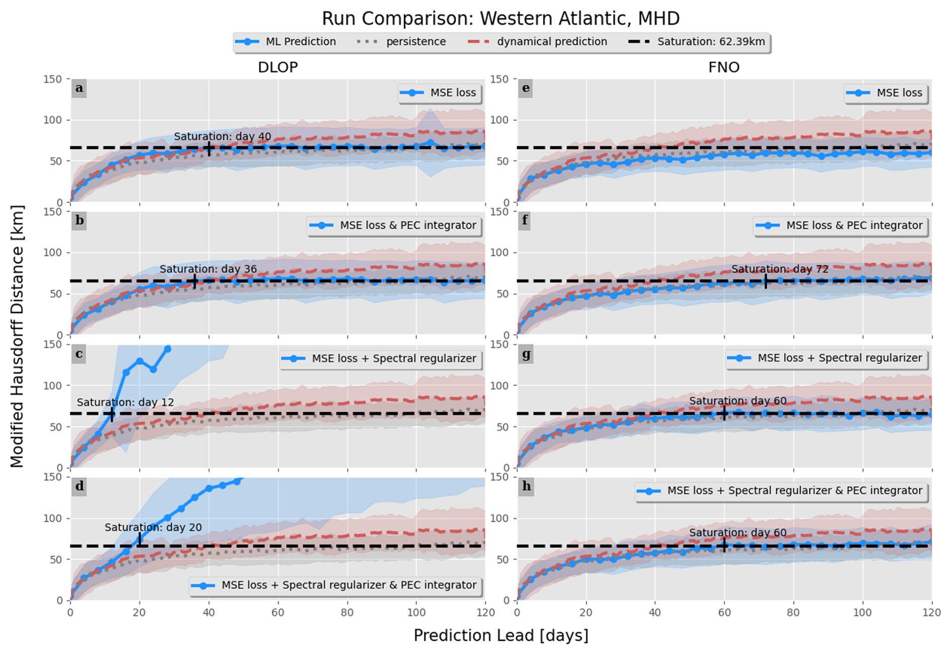
Figure 9 Same as Fig. 8 but for the MHD. The day on which each iteration of the models crosses the saturation value is indicated.

Figure 10 Same as Fig. 8 but for the anomaly correlation coefficient (ACC). The day on which each iteration of the models reaches a value of zero is indicated.

3 Results

This section presents a comparison of mesoscale ocean circulation dynamics represented by the spatiotemporal evolution of SSH fields generated by various iterations of DLOP and OceanNet with the dynamical ROMS forecast using independent reanalysis data. To assess the performance rigorously, both qualitative and quantitative measures are employed. The metrics for evaluating the predictive accuracy of SSH include the RMSE and CC, which are widely recognized and employed in forecasting (Kurth et al., 2023; Bi et al., 2023; Lam et al., 2023; Chattopadhyay and Hassanzadeh, 2023). In addition, a specialized object-tracking metric to evaluate the prediction of major ocean features delineated by SSH contours is incorporated: the modified Hausdorff distance (MHD; Dukhovskoy et al., 2015). The MHD quantifies the comparison of predicted objects to their counterparts between grids; identical shapes at identical locations yield an MHD of zero. To calculate the MHD, at least one shape needs to be identified in each image. For the GSM, the contour identifying the northern frontal boundary of the meander was chosen to be used in MHD calculations. This boundary of the GSM is indicated using a contouring threshold of SSH pertaining to the average SSH across all points in the reanalysis dataset with geostrophic speeds exceeding the average zonal maximum. This SSH contour is approximately −0.17 m. While this defined northern boundary of the GSM is not illustrated by a contour line on most figures, an example of it can be seen in Fig. 1b. The choice of this method for defining the GSM's position proves convenient because it provides a single object that is present in all images – if a contouring level that captures the shapes of individual eddies independent of the GSM is chosen, the calculation of the MHD score becomes tedious due to the possibility of having a mismatch in the number of objects between prediction and validation images. To provide a comprehensive assessment, qualitative snapshots of the predicted SSH fields generated by OceanNet, ROMS dynamical forecasts, and the independent SSH fields derived from the reanalysis are shown.

The ROMS forecasts used for comparison consists of 69 uncoupled 120 d predictions initialized 5 d apart. For fair comparison with the reanalysis dataset, the 5 d mean SSH fields of the ROMS output were compared. As OceanNet has no knowledge of the atmospheric states or ocean boundary conditions during its inferencing, the ROMS forecasts were forced with persistent atmospheric and ocean boundary conditions for each run.

In regional ocean forecasting, defining surface and boundary forcing is a significant challenge, particularly when accurate and continuous global ocean and atmosphere forecasting data for extended periods are unavailable. In this study, persistence refers to the assumption that future conditions will resemble past conditions. While persistence can provide a baseline, it is not expected to capture the full variability or trends in long-term forecasts. We acknowledge the limitations of using persistent forcing to drive ROMS forecasts in this study. This limitation lies not with ROMS, as a dynamical model, but with the specific ROMS forecast configuration that we adopted in this study. An example showing the 2 m air temperature and 10 m wind vectors used to initialize and force a single ROMS simulation is provided (Fig. 4).

A qualitative assessment reveals that OceanNet effectively captures the SSH propagation of undulations in the northern boundary of the GSM (Fig. 5). Moreover, OceanNet skillfully captures large-scale eddies traveling into and out of the domain, even without receiving any boundary information. In contrast, the ROMS dynamical model forecast tends to overpredict SSH and the meridional amplitude of the northern boundary. While it is sensitive to initial conditions, OceanNet remains physically consistent over long-term forecasts in this region. Also, OceanNet provides stable and physically reasonable SSH predictions for the GSM for at least 120 d (not shown for brevity).

For quantitative comparisons, predictions from each model (OceanNet and ROMS) and persistence are compared to the reanalysis dataset to derive metrics at each day of prediction and are presented as averages of the nth day of prediction (Fig. 6). This method allows performance to be evaluated by forecast lead time across various initialization states; an evaluation of the RMSE on the 20th day of prediction is an average measure of model performance with a forecast lead of 20 d given 69 different initial conditions. Each model was also compared to the saturation value of each metric: the 95th percentile of the corresponding metric calculated from 1000 random pairs of images from the entire reanalysis dataset (Delsole, 2004; Dalcher and Kalnay, 1987). If a metric exceeds the corresponding saturation value, the confidence in the prediction is considered to be no more trustworthy than that of selecting a random field of SSH from the reanalysis dataset. It is also important to note that not just the means of the ensemble metrics are investigated, but the corresponding standard deviations of each metric are also considered. If the means of two objects of comparison fall within the standard deviations of each other, not much weight can be put into claiming that one model performs better than the other. In this manner, OceanNet consistently outperforms ROMS with respect to the RMSE, CC, and MHD computed between the predicted SSH values and the reanalysis SSH over 120 d (Fig. 7). Persistence forecasting also fares reasonably well in this region due to the strong background state of the GSM; however, OceanNet can still outperform persistence in all three metrics over 120 d on average. The MHD of OceanNet is shown to cross the saturation value of 62.34 km on day 60, suggesting that the northern boundary of the GSM predicted by OceanNet is no better than selecting a random image from the reanalysis dataset. This is not to say that the position of the entire GSM is off but, rather, that the undulations present in the GSM's northern boundary are completely out of phase. When this is the case, OceanNet does maintain the correct relative position of the GSM, while ROMS frequently places the GSM too far north or south.

The RMSE, anomaly correlation coefficient (ACC), and MHD are compared across different iterations of the DLOP and FNO models, focusing on integration schemes and loss function terms. The two integration schemes compared were the absence of integration (Eq. 6) and PEC. Recall that a difference in integration schemes corresponds to an entire retraining of the model and, thus, results in a different model. The loss function terms compared were MSE and MSE with spectral regularization. This combination of model types, integration schemes, and loss function terms results in eight models to compare, following the same approach as before (ensemble metrics; Fig. 6), against each other and with ROMS and persistence predictions.

The RMSE not only indicates the magnitude of values present but also serves as a measure of accuracy and stability. A high RMSE suggests that the magnitudes in the analyzed field are, on average, less realistic. If the RMSE continues to increase over time, it implies that the model is becoming unstable. In terms of the RMSE, the two DLOP models with spectral regularization included in the loss functions can immediately be identified as becoming unrealistic and unstable within a couple time steps, as they almost immediately cross the saturation threshold and continue to rise (Fig. 8). The two DLOP models with only MSE in their loss function appear to perform well, especially when the PEC integration scheme is present, but the very basic DLOP model with MSE loss and no other augments does appear to become unstable around day 100. Out of all the DLOP models, the only one with a competitive RMSE at all time steps is the iteration with PEC integration and MSE loss. For the FNO model, all combinations of integration schemes and loss function terms are approximately the same; however, they all show a slightly higher RMSE at day 60, which continues to increase in time, than the DLOP model with PEC integration and MSE loss.

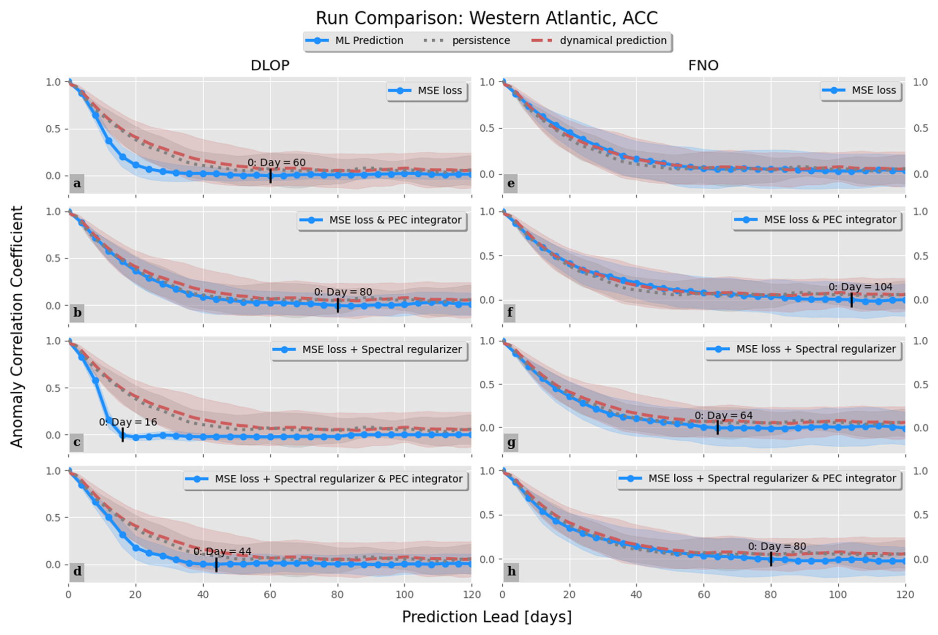
The plots regarding the RMSE are a great initial impression of performance, but other metrics are important to consider when choosing the best model. That said, the MHD plots tell a similar story to the RMSE, with the only differences to note being as follows: (1) DLOP with MSE loss does not become unstable in terms of MHD and (2) all of the FNO models remain under the saturation value for longer than the two best DLOP models identified in the RMSE plots (Fig. 9). Taking the analyses of the RMSE and MHD together, it seems as though the best model may be any of the FNOs or DLOP with MSE loss. The final metric investigated is the ACC. Like the CC, the ACC is a comparison of how closely correlated two sets of data are, but the ACC considers the field with the long-term point-wise mean removed prior to comparison. The removal of the long-term mean allows comparison of the two datasets on a finer scale. From the ACC, the results of the RMSE and MHD analyses are confirmed, and the qualifying best models are selected to be any version of the FNO and the DLOP model with PEC integration and MSE loss, as these models are at least competitive with the ROMS predictions across all time steps in all three metrics (Fig. 10). This is the extent of the analysis possible from the provided metrics; thus, to identify the absolute best model, one must compare the actual fields of SSH predictions produced by each model to ensure that they make physical sense.

While there are four versions of the FNO model which, metrically, appear to be competitive, extensive hyperparameter tuning and subsequent verification revealed the best of these to be the FNO with PEC integration and MSE loss with spectral regularization. This model, with the addition of the two-time-step loss described in Sect. 2.4.1, became what is presented here as OceanNet. Covering the individual results of hyperparameter tuning each FNO model and then comparing the verification of their physical fields is beyond the scope of this paper. An example prediction of a single instance of prediction with a lead of 40 d made by the best DLOP model, ROMS, and the finalized OceanNet model is shown to demonstrate the difference between the physical fields predicted by each type of model (Fig. 11).

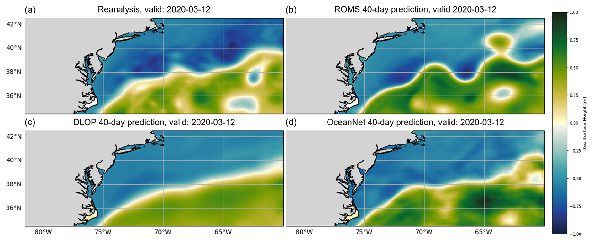
Figure 11 Predictive performance of DLOP, ROMS, and OceanNet on the GSM region at 40 d. The SSH field 40 d after model initialization on 1 February 2020, as described in Sect. 3, for (a) the reanalysis dataset, (b) ROMS, (c) DLOP, and (d) OceanNet.

4 Discussion and conclusions

This study demonstrates the capabilities of the neural-operator-based OceanNet: a data-driven machine learning model for GSM prediction over subseasonal to seasonal timescales. The techniques explained throughout Sects. 2.3 and 2.4 (FNO, PEC integration, spectral regularization, and multi-time-step criterion) mitigate autoregressive error growth and the spectral bias seen in other data-driven architectures, making OceanNet a solid candidate to function as a digital twin for long-term regional ocean circulation simulations.

Using high-resolution SSH data for the years 1993 through 2018, OceanNet was trained to predict ocean states with a 4 d lead time. The ability of OceanNet to autoregressively forecast the mesoscale ocean processes of the GSM over 60–120 d was evaluated by standard metrics used in machine learning and oceanographic communities. The results of this study provide two main conclusions: (1) OceanNet remains remarkably stable over many iterations of autoregressive prediction and (2) the model consistently outperforms ROMS dynamical forecasting across various initial ocean states in terms of RMSE, CC, and MHD. In addition, an inherit advantage of machine learning models in general are their ability to inference at tremendous speeds (4 000 000 times faster, in this case). These results demonstrate the potential of utilizing scientific machine learning to develop long-term, stable, and accurate data-driven ocean models of great computational efficiency, paving the way for realizing a data-driven digital twin encompassing the entire climate system.

While the skill of OceanNet is impressive, the conclusions presented here are not without limitations. This study was conducted and trained on a single ocean feature, with a single spatial and temporal scale, from a reanalysis dataset utilizing only a single variable. Real-world ocean forecasting systems operate with full-physics dynamical ocean models and real-time observational ocean data, covering dynamical processes across diverse spatial and temporal scales. The disparities between these data sources and scales necessitate further investigation into OceanNet's performance across various ocean applications. The comparisons between OceanNet and ROMS can also be considered to have a major caveat: ROMS, as a regional ocean model, depends on providing forcing conditions on the ocean surface and at open boundaries, for which persistence was provided in this study. This method would not be used in conventional prediction scenarios over the timescales considered here; as such, it may be more fair to compare the performance of OceanNet to a model that does not require boundary conditions, such as a global ocean model, or to a configuration of ROMS forced with forcing and boundary conditions taken from predictions produced by a global model. The use of a global model would be expensive due to the resolution that OceanNet uses, so perhaps the best comparison could be done once OceanNet is expanded to cover the global ocean as well. Efforts by our research team to apply OceanNet to the global ocean are currently underway and will be reported in a future correspondence. In the meantime, the potential for OceanNet to include multiple state variables, such as surface currents, temperature, or even depth-averaged variables, could improve the prediction of smaller-scale circulations and events, such as shelf break jets and frontal currents, and provide more variables to compare to numerical methods. In addition, OceanNet produces very smooth, continuous fields which can potentially lead to an underestimation of the magnitudes of extreme ocean events; therefore, additional research is imperative to assess OceanNet's performance under extreme ocean conditions, e.g., during severe storms.

Significant opportunities exist for improvement in both AI-based methods and dynamical model-based ocean forecasting. In the AI domain, potential advancements involve the integration of subsurface ocean states and additional ocean variables, the incorporation of temporal dimensions through the training of 4D deep networks, and the exploration of more complex network architectures with increased depth and breadth. In the realm of numerical ocean forecast modeling, the development of pre- and post-processing techniques can help mitigate the inherent biases found in ocean models. We expect that a hybrid approach, combining data-driven and dynamical numerical models, will play a pivotal role in pushing the boundaries of excellence in ocean prediction.