the Creative Commons Attribution 4.0 License.
the Creative Commons Attribution 4.0 License.
 | 12 Jan 2024
Technical note: Extending sea level time series for the analysis of extremes with statistical methods and neighbouring station data
Morten Andreas Dahl Larsen
Martin Drews
Erik Nilsson
Anna Rutgersson
Extreme sea levels may cause damage and the disruption of activities in coastal areas. Thus, predicting extreme sea levels is essential for coastal management. Statistical inference of robust return level estimates critically depends on the length and quality of the observed time series. Here, we compare two different methods for extending a very short (∼ 10-year) time series of tide gauge measurements using a longer time series from a neighbouring tide gauge: linear regression and random forest machine learning. Both methods are applied to stations located in the Kattegat Basin between Denmark and Sweden. Reasonable results are obtained using both techniques, with the machine learning method providing a better reconstruction of the observed extremes. By generating a set of stochastic time series reflecting uncertainty estimates from the machine learning model and subsequently estimating the corresponding return levels using extreme value theory, the spread in the return levels is found to agree with results derived by more physically based methods.
- Article
(3055 KB) - Full-text XML
- BibTeX
- EndNote


Extreme sea levels (ESLs) can have disastrous consequences in coastal zones in terms of flooding vulnerable assets, loss of lives, and disturbances (Brown et al., 2018; Vousdoukas et al., 2020; Wahl et al., 2017). Coastal floods generally result from a combination of ESLs, wind, waves, tides, and local conditions, including bathymetry and terrain features. Climate change also affects ESL events due to sea level rise and changes in storm frequency and/or intensity (Rutgersson et al., 2022). Reliable estimates of current and future ESLs are urgently needed to mitigate the impacts of disaster risks and to inform adaptation to climate change. Long time series of observed sea levels are essential for improving confidence in statistically inferred return levels (RLs) (Menéndez et al., 2010; Woodworth et al., 2011) and are often considered essential for coastal planning. International initiatives such as the Global Sea Level Observing System (GLOSS) (Caldwell, 2012; Merrifield et al., 2012) and other works (Woodworth et al., 2010) have highlighted this necessity and called for the recovery of historical records in what is known as “data archaeology”. Nevertheless, the temporal paucity of sea level time series (Holgate et al., 2013) remains a limitation for adequately estimating RLs and ESLs in many places.
This technical note evaluates a machine learning method called random forest (RF) (Breiman, 2001) for extending the sea level time series obtained by a tide gauge of interest using a longer time series at a neighbouring tide gauge in the context of analysing sea level extremes. This is particularly relevant when the initial time series is very short, e.g. in the order of ∼ 10–20 years, which is principally too short to allow reliable statistical inference of ESLs (e.g. a RL corresponding to a 100-year event). The RF methodology is compared to a linear regression (LR) model, which could also be expected to perform adequately for short time series.
Our study area lies within the Kattegat Basin, located on the western coast of Sweden, around the city of Halmstad (Fig. 1). Here, according to the Swedish Meteorological and Hydrological Institute (SMHI), the highest recorded Swedish sea level of 235 cm was observed in November 2015. This event was mainly due to local conditions leading to a sea level increase of 50–100 cm in comparison with neighbouring stations, such as Viken; however a seiche effect could also have added around 25 cm to the total sea level (Johansson, 2018). In this area, tides vary with an amplitude of around 20 cm during spring tides (Svansson, 1975), and current ESLs are mainly due to storm surge effects. However, other factors could also play a role, such as the preconditioning of the Baltic Sea (Andrée et al., 2023). Hieronymus and Kalen (2020) showed that the Swedish western coast is expected to be one of Sweden's most exposed areas due to rising sea levels.
Different methods have been proposed to extend sea level records. For example, Bernier et al. (2007) used short observation time series associated with a 40-year hindcast surge model. Reconstructions by Cid et al. (2018) were based on tide gauge data and atmospheric conditions. Hieronymus et al. (2019) showed good performance of neural networks with respect to predicting sea levels at tide gauges located along the Swedish coast based on different atmospheric variables and tide gauge records. Granata and Di Nunno (2021) found similar results when forecasting tides in the Venice region using different machine learning methods, including RF, regression tree, and multilayer perceptron. Recently, Bellinghausen et al. (2023) demonstrated the utility of using an RF classifier to satisfactorily predict the occurrence of ESLs at a few stations around the Baltic Sea within 3 d based on surface wind and pressure fields, precipitation, and the pre-filling state of the Baltic Sea.
In the following, we systematically evaluate the performance of RF as means of extending a very short time series of only 10 years and of reconstructing past sea level variations based on a more extended time series from a neighbouring station. This approach is compared to the linear regression approach. Both methods have previously been found to reduce biases efficiently and are relatively computationally inexpensive with low complexity when applied to a small number of input variables, as is the case in this study. To evaluate the sensitivity of the reconstructed sea level with respect to the geographic distance from neighbouring stations, we apply the method to data from different stations. Finally, we consider the method's potential and limitations with respect to the reconstruction of sea level extremes when the time series of interest is very short and inherently provides a poor sampling of even moderately extreme events.
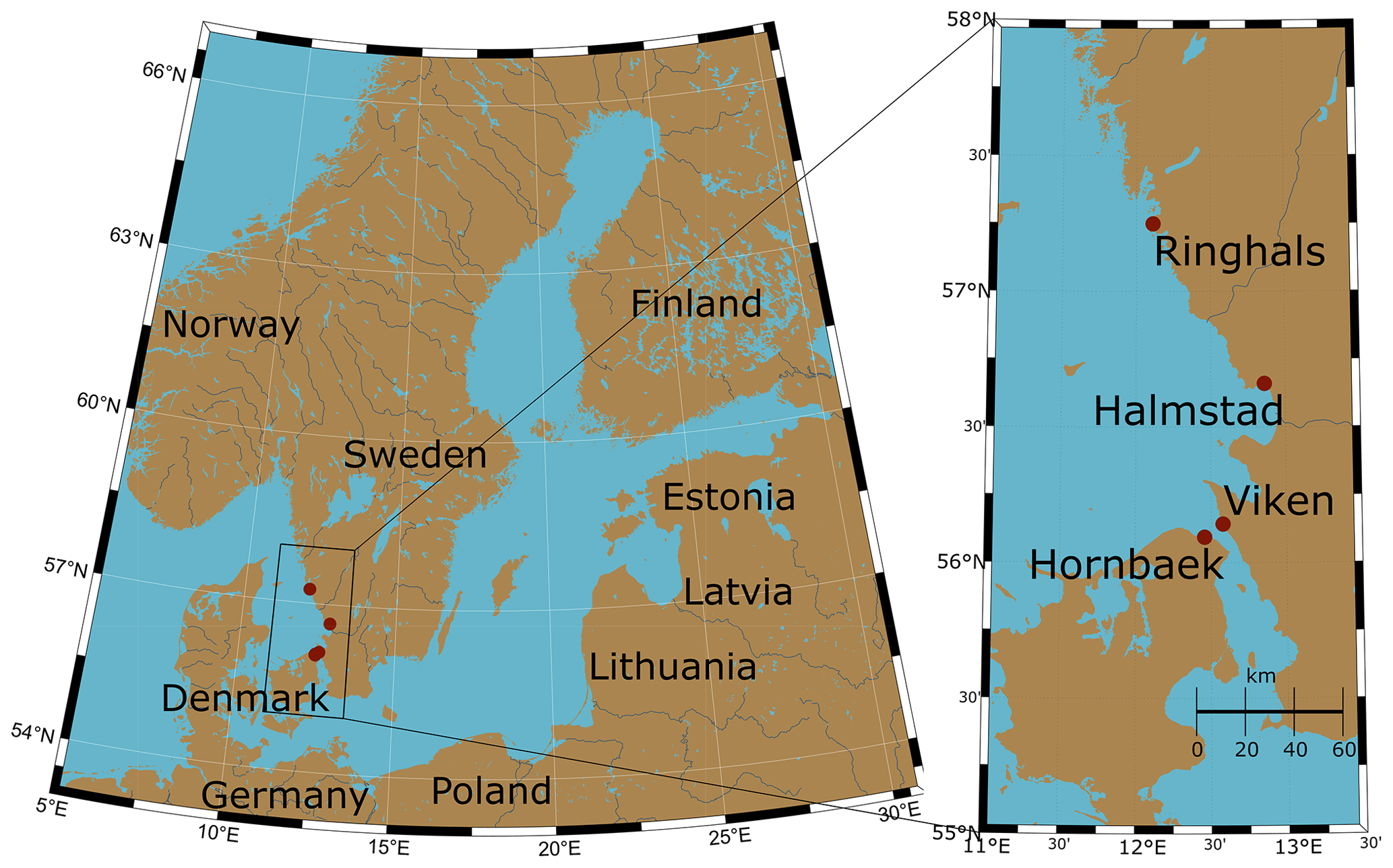
Figure 1Map of northern Europe indicating the study area and the tide gauge stations (red dots).
2.1 Sea level data
The datasets used in the analysis are hourly sea level observations from different stations available from SMHI (SMHI, 2021) and the Danish Meteorological Institute (DMI). Three stations are located on the western coast of Sweden – Ringhals (station no. 2105, “RINGHALS”), Halmstad (station no. 35115, “HALMSTAD SJÖV”), and Viken (station no. 2228, “VIKEN”) – and one station is located on the east coast of Denmark – Hornbæk (Hansen, 2007) (Fig. 1). The distance between Hornbæk and Viken is around 9 km, the distance between Hornbæk and Ringhals is around 130 km, and the distance between Viken and Ringhals is around 127 km (Table 1). The geographical location of the stations is important, as it can change how the water level behaves, for example, stations may be constricted in a channel, such as Viken and Hornbæk. Here, ESLs are defined as the total highest measured sea level including tides and storm surges; this choice is motivated by the low tidal range in the area (Svansson, 1975).
Each hourly time series is first linearly detrended and transformed into a time series of daily maxima from which the annual maximum is determined for each year in the series. When determining the annual daily maximum, we enforce a minimum temporal separation of 2 d to ensure the independence of events at each station. The datasets are of varying lengths (Fig. 2), ranging from 12 years (Halmstad station) to 129 years (Hornbæk station). Long-term linear trends (i.e. sea level rise) were estimated over the whole time series for all stations and found to be 0.33 cm (Ringhals), 0.35 cm (Hornbæk), 1.47 cm (Viken), and 5.51 cm (Halmstad) per decade.
After being detrended, the Hornbæk sea level varied from −145 to 187 cm, the Viken sea level ranged between −114 and 166 cm, the Ringhals sea level ranged between −105 and 162 cm, and the Halmstad sea level ranged between −94 and 213 cm relative to the mean sea level (Fig. 2).
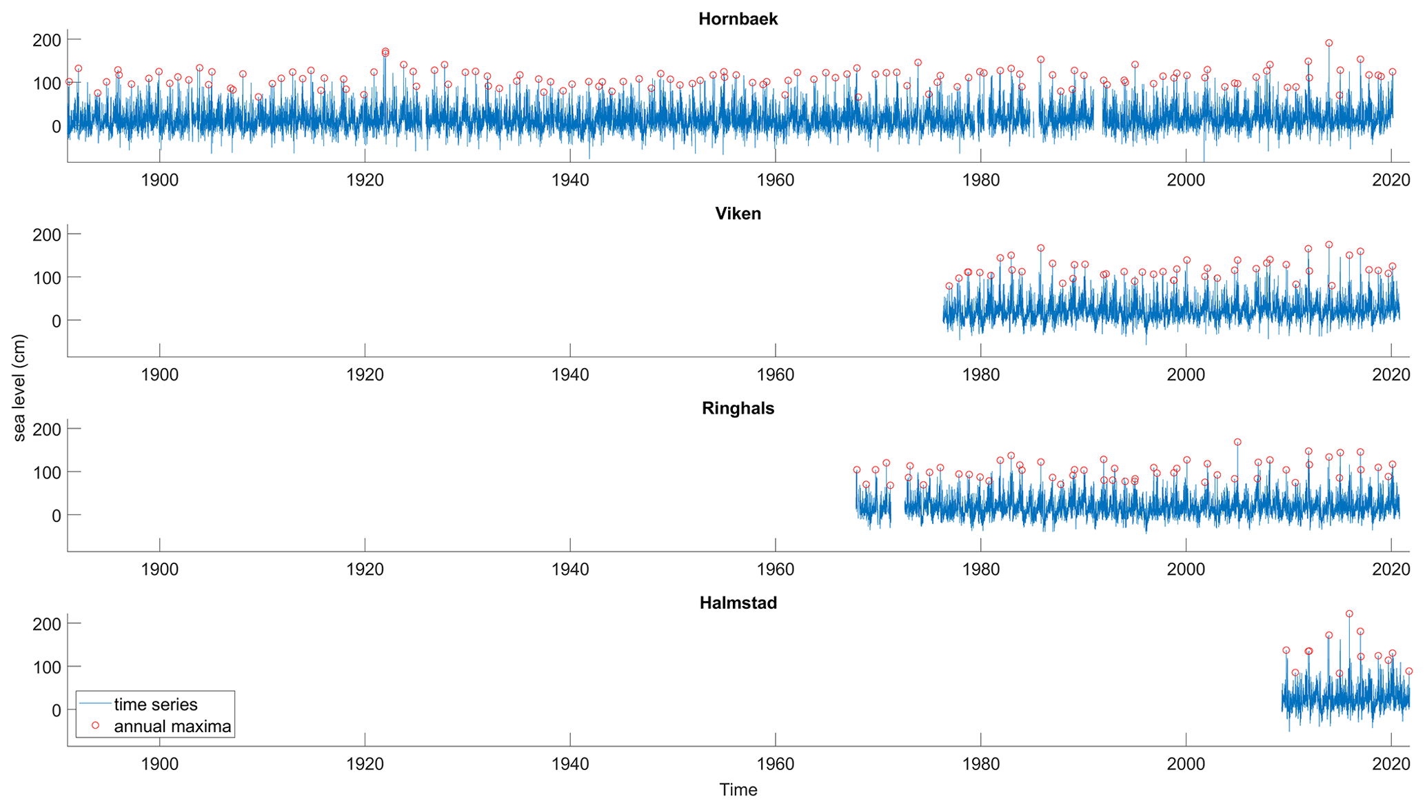
Figure 2Sea level time series from the four tide gauge stations showing daily maximum values (blue) and yearly maximum values (red circles).
2.2 Methods
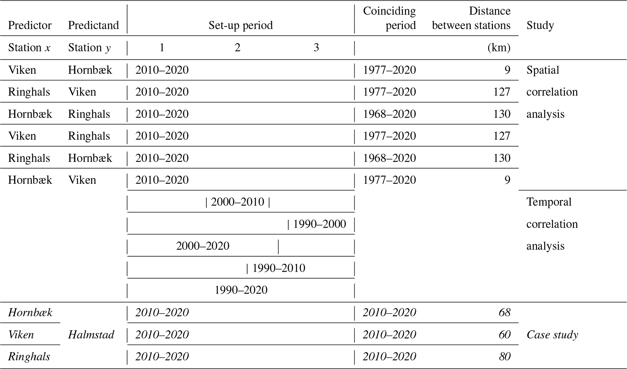
The proposed approach for temporally extending short observed sea level time series at the station of interest (y) is based on using longer observed sea level time series at a neighbouring station (x) constituting the predictor. For each x–y station pair (Table 1), we use a temporally coinciding time series to set up each prediction model (e.g. 10 years). We will refer to this as the “set-up period”. Within the set-up period, models are fitted or trained using both time series for 80 % (8 years in our example) of overlapping data (training dataset), whereas the last 20 % (2 years in our example) serve as the validation dataset to provide an unbiased evaluation of the model fit. The coinciding period outside of the set-up period constitutes the testing period. Two overall predictor approaches are employed: one using simple LR and one based on RF machine learning.
For both approaches, we only use the sea level of the daily maxima at station y at time t, denoted as yt, predicted from the sea level at station x at time t, denoted as xt. Nevertheless, as the sea level is sensitive to meteorological conditions, which are advected by the winds, the sea level at one station at time t might be better predicted using the time-lagged sea level from another station, e.g. the sea level at time t± a few days. Here, we use the daily maxima, which might buffer this effect to some extent. However, it is most likely that some slight improvements could be found when applying some time-delayed variables. Therefore, a short analysis has been done to test time-lagged variables for the set-up period of 30 years for each x–y station pair. Three different tests have been done. The first one, in which no time-delayed predictors were added, is the one used in this paper: yt= RF(xt). In the second one, we add two time-delayed variables, time t−1 d and time t−2 d: yt= RF(xt, xt−2, xt−1). In the third one, we add four time-delayed variables, time t−1 d, time t−2 d, time t+1 d, and time t+2 d: yt= RF(xt, xt−2, xt−1, xt+1, xt+2). Slight improvements in the root-mean-square error (RMSE) values (around 1–2.5 cm) and r values (around 0.03–0.08) are found for all x–y station pairs, with the best test being the third one, although the second one also presented intermediate improvement. Bias values barely changed, with maximum changes of 0.2 cm; however, towards the extremes, values from tests 2 and 3 presented a bigger underestimation than those from test 1. Thus, for this study, we believe that the method used within the paper (test 1) is sufficient and might even be the best method to reproduce ESLs. This might be due to the fact that RF is statistically based and is only applied to stations in close proximity to each other (max 130 km) that are, therefore, mostly submitted to the same synoptic atmospheric phenomena within 1 d of one another. More testing could be done to really assess the potential added value of using time-delayed variables, but this is outside of the scope of this study.
2.2.1 Linear regression
Based on each x–y predictor–reconstruction station pair, a linear equation is found using the least-squares method as means of determining the best-fit coefficients. Based on the resulting equation, yt is predicted from xt.
All coefficients values from the linear fits are positive and fairly close to 1 (0.765–1.12), meaning that a low sea level at one station corresponds to a low sea level at another station; a similar effect is also then found for high and intermediate sea levels. Therefore, the sea level at one station varies at a rather similar rate to the other station, as a coefficient value of 1 would mean that the sea level measured at one station would be increasing or decreasing as the same rate at another station. The x_Hornbæk–y_Halmstad set presents a coefficient that is closer to 1, highlighting a strong correlation between those two stations. Only the x_Ringhals–y_Halmstad and x_Viken–y_Halmstad station pairs present a coefficient higher than 1. This suggests that the sea level at Halmstad varies at a higher pace than at the two predictor stations.
2.2.2 Random forest
A probabilistic RF model is trained using the sea level at one station as the predictor (x) and the sea level at another station as the predictand (y). The RF method yields a mean and a standard deviation for each predicted value (Breiman, 2001). The RF model is implemented using the TreeBagger (https://se.mathworks.com/help/stats/treebagger.html, last access: 20 April 2023) MATLAB function, in which the regression method is based on a number of trees and minimum leaf size hyperparameters. The mean and standard deviation values are predicted using the predict (https://se.mathworks.com/help/stats/treebagger.predict.html, last access: 20 April 2023) MATLAB function. We use the predict function for our regression problem; in the MATLAB documentation, there is a further description of the function for the weighted average of the prediction using selected trees. We do not use the TreeWeights option, but we do employ the output of the standard deviations of the computed responses over the ensemble of the grown trees for regression: [Yfit,stdevs] = predict(B,X). Here, Yfit is a vector of predicted responses for the predictor data in the table or matrix X, based on the ensemble of bagged decision trees B. By default, the predict function takes a democratic (non-weighted) average vote from all trees in the ensemble. Here, these parameters are set to 500 and 1, respectively which were values chosen after a brief sensitivity analysis and are not the default choices for regression models. The LR is fitted and the RF model is trained using the same set-up period for each station pair (Table 1).
2.2.3 Model testing
To evaluate the proposed methodology, different analyses with different combinations of stations are used to test the spatial and temporal sensitivity (Table 1). Six analyses using different combinations of station data obtained at Hornbæk, Viken, and Ringhals are carried out using the recent 10 full years (2010–2020) as the common set-up period for model training and validation (see Sect. 2.2.2). Six additional analyses are carried out to predict Viken sea levels from Hornbæk data using the two previous time periods (2000–2010 and 1990–2000) as well as using a 20-year set-up period (1990–2010 and 2000–2020) and a 30-year set-up period (1990–2020) for training and validation to evaluate the temporal sensitivity. All 36 possible combinations have then been analysed to better estimate the spatial and temporal sensitivity. Finally, we compare the reconstructed sea levels at Halmstad using the station data from Hornbæk, Viken, and Ringhals, respectively (see Sect. 3.2), for the period from 2010 to 2020. In the latter case, we also estimate RLs based on the reconstructed time series and compare them to previous results reported for Halmstad.
To assess the performance of each model, different goodness-of-fit (GOF) metrics are chosen: the root-mean-square error (RMSE) and the Pearson correlation coefficient (r). Moreover, the general bias (bias) and the 95th percentile bias (perc95-bias) between the observations and both model reconstructions (LR and RF) within the validation period are calculated.
To evaluate the model's performance towards the extremes, annual maxima and values above the 95th, 97th, and 99th percentiles from observations are compared with the corresponding predicted values.
Table 1Experimental set-up and summary of analyses. The case study of Halmstad city is highlighted in italic.
2.2.4 RF method with random sampling to evaluate RLs
The RF method estimates the standard deviation associated with the predicted sea level daily maximum at each time point. We denote the following introduced methodology as the “RF method with random sampling”. Based on the RF daily means and standard deviations, we select the corresponding annual maxima from the reproduced time series and their associated standard deviations. We assume that a Gaussian distribution describes the probability for each predicted annual maximum. RLs are subsequently calculated using a generalized extreme value (GEV) distribution fitted to the annual maxima (Coles, 2001). This yields an ensemble of randomly drawn RL curves. The 95th percentile of the ensemble spread is calculated.
We denote x, the predictor time series of daily maxima; y, the predicted time series of daily maxima; and SDy, the standard deviation associated with y which is obtained by = RF(xt) at time t with RF, the trained RF model.
We can then extract the time series of annual maxima from the mean predictions and its associated standard deviation (which we denote as Yn and , respectively) with , where N is the number of years in y. Let us introduce a random variable R that is distributed normally:
Therefore, for each annual maximum, we can then randomly get a value that gives us one set of N annual maxima values. We then repeat this operation 10 000 times to get 10 000 sets of N randomly obtained annual maxima. We next fit a GEV distribution for each set, which ultimately gives us 10 000 randomly drawn RL curves. This is what we call the ensemble spread, from which we extract the 95th percentile to get a reasonable uncertainty spread.
This method is further compared with the commonly used GEV approach applied directly to the N-year annual maxima of the predicted mean values from the RF model, which we simply refer to as RF.
3.1 Model validation
To validate the models, GOF metrics are calculated (and partly presented in Table 2). For the time series of daily maxima, roughly similar statistics are found for all datasets, irrespective of whether the RF or LR is used. In general, we find slightly (but not significantly) better r and RMSE values associated with the LR and a slightly better perc95-bias for the RF (not shown). For the annual maxima, the 95th, 97th, and 99th percentile sets show marginally higher r and lower RMSE values for the LR in nearly all cases, with a maximum difference of 4 cm for the RMSE (except for 4 simulations of the 36 where RMSE values vary by up to 10 cm towards the extremes) and 0.10 for the r value. Overall, RMSE values are between 10 and 40 cm and r values are between 0.4 and 0.9 in most cases when looking at the extreme sets. Smaller RMSE values ranging from 5 to 15 cm and r values above 0.75 are found when looking directly at the predicted time series. Hence, error metrics are generally worse for both methods when calculated for extreme values (annual maxima and high percentiles) compared with the overall values calculated from the full time series of predicted daily maxima values. For extremes, represented by the high-percentile datasets, bias values range from −30 to −2 cm, i.e. an underestimation of the observed extreme values for both the LR and RF. As shown in Table 2, biases vary, with a maximum difference between models of ∼ 10 cm in almost all cases. This highlights the fact that both models lose accuracy with respect to predicting ESLs compared with predicting less extreme events. This seems to be caused by the non-linear effects occurring during the extremes, as the decrease in r shows. Figure 3 depicts the correlation between observations and models with respect to predicting Viken sea levels from the Hornbæk data trained on the 2010–2018 period. A similar picture is observed in nearly all cases (not shown). As shown in Fig. 3, the RF model returns significantly higher sea levels and shows higher variability towards the most extreme range compared with the LR, except when predicting Hornbæk sea levels from Viken data, where the model is trained on observations from the 1990–2000 and 2000–2010 set-up periods (not shown). In those two cases, the RF does not correctly reproduce the extreme range (as they are out-of-sample data, whereas the predicted values are bounded) because it can only reproduce in-sample events; however, those events correspond to the highest ESLs, which the LR also struggles to reproduce, and the RF, therefore, does not give much lower values than the LR in this case. This effect disappears when the model is trained on a longer time period, as we could see when investigating at the 20- and 30-year set-up periods (not shown). Compared with the LR, it is clear that the inherently non-linear RF is better able to account for the few moderate extremes that occur during the 8-year training period, whereas they are likely to be suppressed in a linearized model.
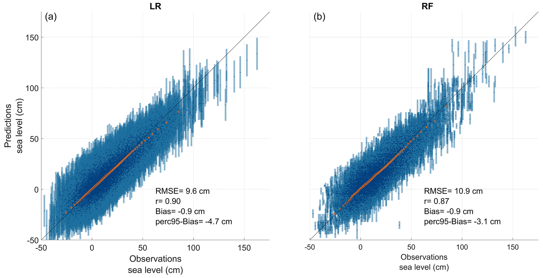
Figure 3Scatter plot between observations and the LR (a) and RF (b) for predicting Viken sea level (y) from the Hornbæk tide gauge (x) for the set-up period from 2010 to 2020. Blue points show the daily maxima, each corresponding blue bar shows the standard deviation, and coloured stars correspond to percentile values ranging from the 1st percentile to the 99th percentile of the dataset.
Table 2RMSE and bias values between different datasets evaluated in the validation period. Noticeable improvements (> 5 cm) in terms of model bias with respect to annual maxima using the RF model are highlighted in bold. A negative bias corresponds to an underestimation of the predicted values, whereas a positive bias (italic) corresponds to an overestimation. Error metrics calculated over the testing period for the case study of Halmstad city are displayed in bold italic. Because of the short length of the testing period, we do not calculate the bias on the annual maxima.
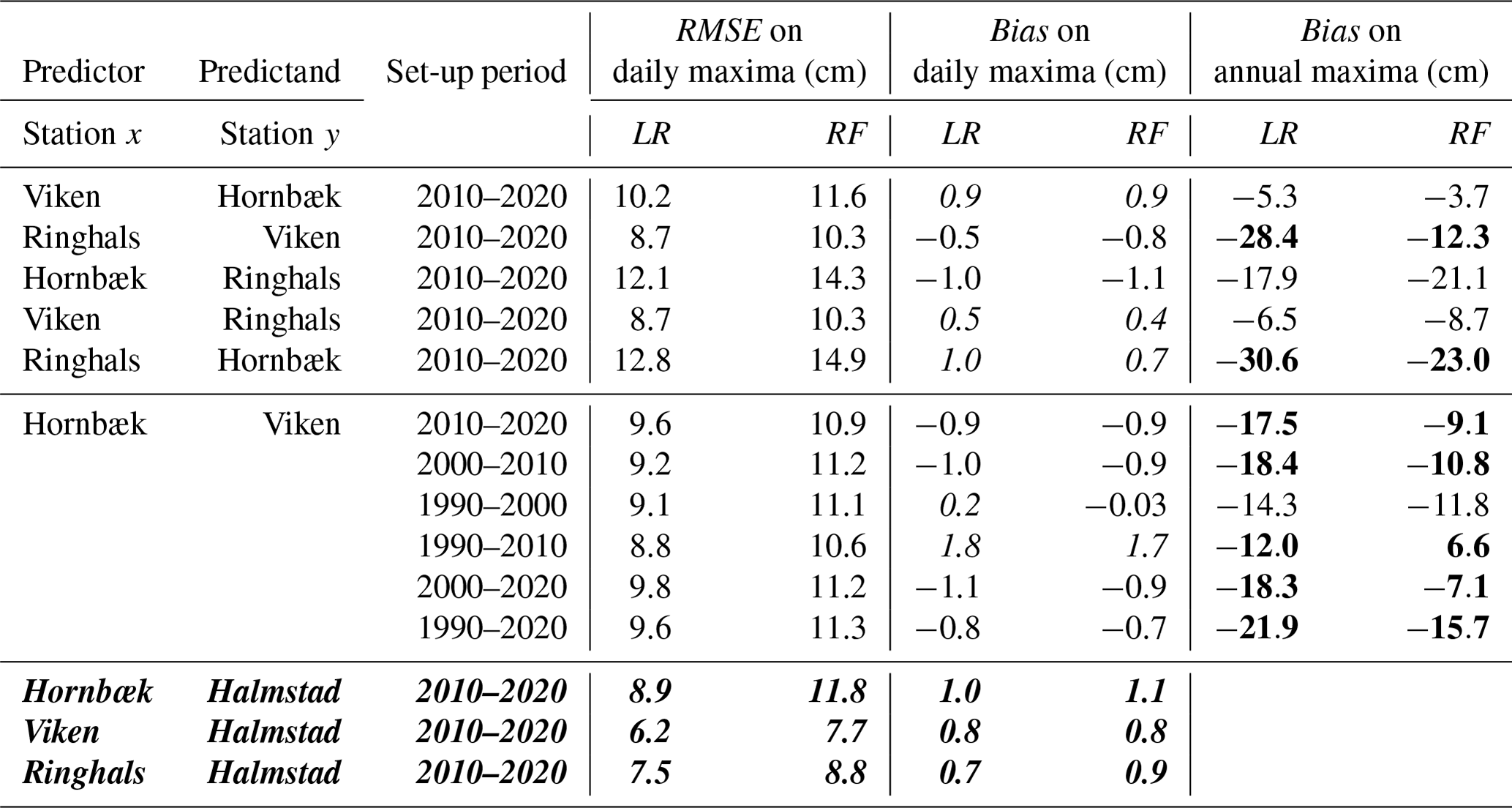
Table 2 analyses the sensitivity to the distance between the two tide gauges for the 2010–2020 period. When the distance between two stations grows, the accuracy of both models seems to decrease, especially towards the extremes. For example, when looking at daily maxima values as well as the extreme set values, RMSE values of around 8–20 cm and r values of around 0.7–0.9 are found for the sets reproducing the Viken sea level from the Hornbæk tide gauge and its mirror set (9 km apart), compared with RMSE values of around 12–40 cm and r coefficients of around 0.3–0.8 when reproducing the Ringhals sea levels from Hornbæk data and its mirror set (130 km apart) (Table 2). The highest differences are also observed for the extremes (annual maxima or the 95th, 97th, and 99th percentiles). Similar results are found when comparing the sea level time series for Hornbæk and Ringhals based on Viken data and when comparing predictions for Viken and Hornbæk sea levels based on Ringhals data (not shown). When comparing results from mirrored sets (e.g. when predicting Viken sea levels from Ringhals data or predicting Ringhals sea levels from Viken data), we do not always find the same performance, especially towards the extremes, as measured by the GOF metrics. This can probably be explained on physical grounds due to localized phenomena resulting, for example, from the topography or the local meteorological conditions; however, this is beyond the scope of the current technical note. Indeed, there are two sets of stations with very significant geographical differences: Hornbæk and Viken stations lie inside of a channel (almost at the entrance), whereas other stations are located on the open coast. In general, the RF method seems to be more accurate than the LR when predicting ESLs, for which it is essential to capture the non-linear behaviour and variability associated with the complex natural interactions between the drivers of ESL events. The non-linear behaviour and variability are likely to become more prominent when observations are obtained at sites further away. Conversely, LR is inherently constrained by a linearity assumption.
3.2 Halmstad
The highest sea level recorded in Sweden occurred in Halmstad, indicating that Halmstad is highly susceptible to ESLs. However, the length of the local sea level time series is very short. Subsequently, three stations – Hornbæk, Viken, and Ringhals – are used to reconstruct the Halmstad sea level time series (Table 2). As shown above, using an RF or LR method, we can, in principle and with reasonable confidence, reconstruct Halmstad sea levels back until 1891 for the period before observations became available in 2009 using Hornbæk station as a predictor, as it has the longest observed time series.
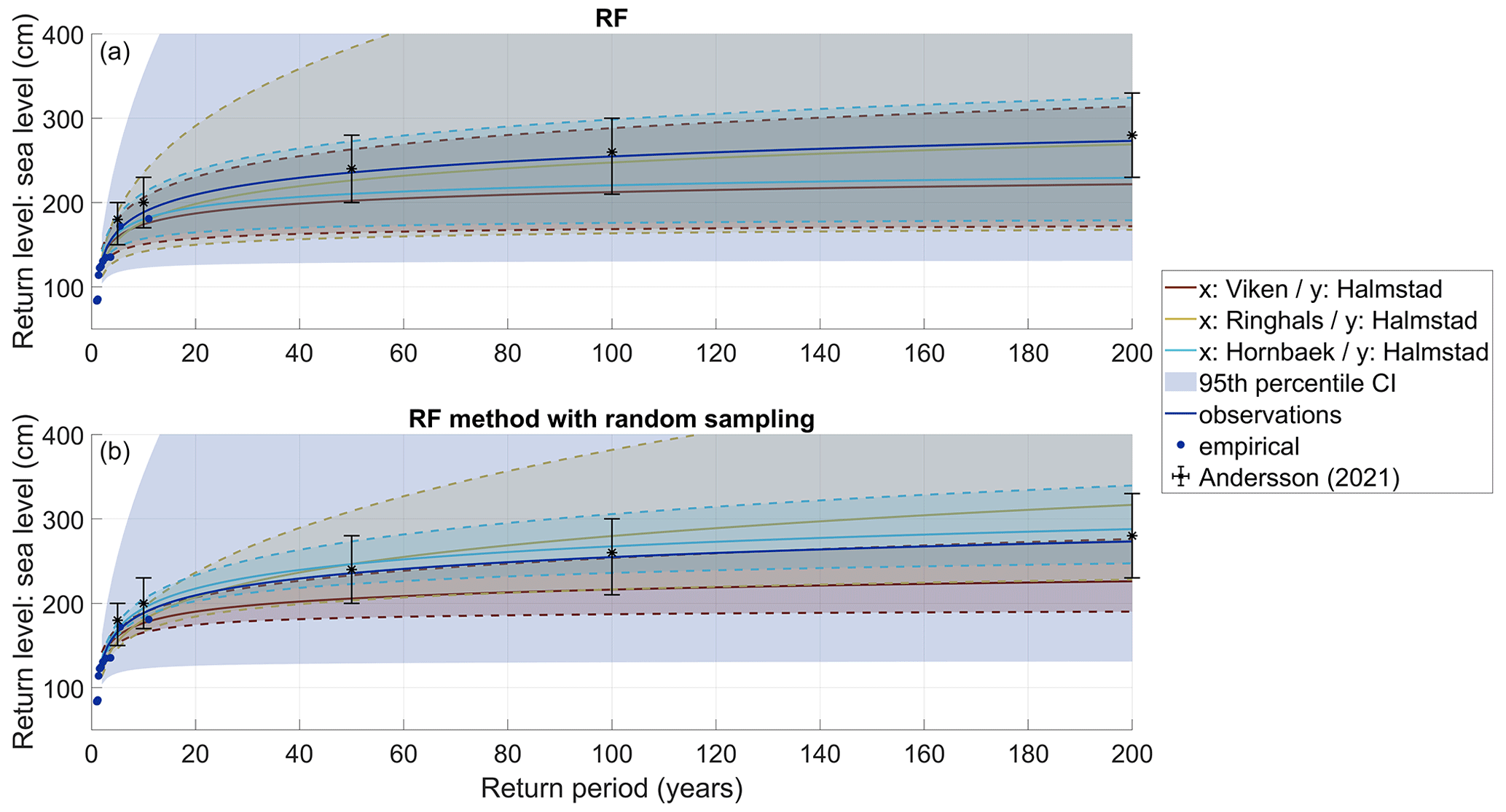
Figure 4RLs from each reconstructed time series to predict the sea level for Halmstad based on RF model mean outputs (a) and following the RF method with random sampling (b). The figure displays maximum likelihood estimates of the GEV distribution fits of each dataset associated with 95th percentile confidence intervals (CIs) (a) and the 95th percentile ensemble spread (b) in background colours, while the dots represent the empirical data from observations. Black error bars show RLs and the 95th percentile CIs calculated from Andersson (2021).
Because of the short length of the Halmstad time series, the training period is almost identical to the full time series; in practice, this makes it difficult to assess the model behaviour on extremes. Therefore, we used different 2-year testing and 8-year training periods to analyse how the model behaves for Halmstad station (the set-up period was from 2010 to 2020 with different testing periods: 2010–2012, 2011–2013, 2012–2014,..., 2017–2019, and 2018–2020); this has also been done to predict the Halmstad sea level from Hornbæk, Ringhals, and Viken separately. Overall, the difference between each testing period is rather small, with RMSE values ranging from 1.5 to 4.1 cm, r values ranging from around 0.03 to 0.06, a bias from 5.2 to 6.8 cm, and a perc95-bias ranging from 5.4 to 16.5 cm. We found that, as in the other simulations done (predicting Viken from Hornbæk for example), the RF visually (from correlation plots; not shown) behaves better towards the extremes (at least slightly) than the LR for all sets and tests, except for the testing period from 2015 to 2017 when predicting Halmstad from Viken or Hornbæk. Furthermore, between the LR and RF, RMSE values only vary by a maximum of 2.9 cm (x_Hornbæk–y_Halmstad) or 1.9 cm (in the two other sets). The x_Viken–y_Halmstad set has the lowest RMSE values, with an average across the simulations of 6.4 and 7.9 cm, a bias of −0.2 and −0.4, and a perc95-bias of −2.7 cm in both the LR and RF, respectively. Therefore, it seems that the model behaves relatively well on extremes for Halmstad station, even though we cannot fully ensure its behaviour because of the short length of observations. Moreover, this conclusion is partly reinforced by the analysis between surrounding stations where the testing could be done over a larger time period using the 2018–2020 period as testing with the 2010–2020 period as the set-up period.
In previous studies, Halmstad's RLs have been calculated for current and future climate scenarios based on reconstructed sea levels from local wind speed observations of the Nidingen offshore station and Viken tide gauge data (Andersson, 2021). For Halmstad, RLs based on extended time series using the three neighbouring stations permit a reduction of the 95th percentile confidence interval (CI) compared with observations. Here, the full-period length of Halmstad's observed values (station y) are concatenated with the predicted time series to get the longest and more accurate extended time series possible before a GEV fit is applied. Even so, RLs are still lower, although they are within the uncertainty range of those displayed by Andersson (2021), which is a good sign, except for the 200-year RL with Viken as a predictor when based on the RF mean outputs (Fig. 4a, Table 3). This could possibly be explained by the underestimation found towards the extremes on the predicted and, therefore, extended time series. This is why we introduced the RF method with random sampling which allows us to represent more extreme values.
Table 3Halmstad's RLs from reconstructed time series using the outputs from the RF method and the RF method with random sampling applied to the Hornbæk (italic) station compared with the assessment by Andersson (2021; bold italic).
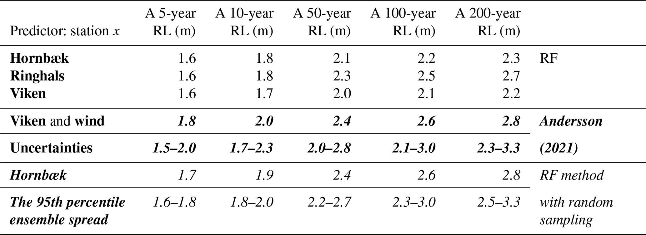
Conversely, we apply RF-based random sampling to predict RLs probabilistically, as described in Sect. 2.2.4 (Fig. 4b), at Hornbæk, Viken, and Ringhals (which results in an extended time series of around 120 years, 35, and 45 years, respectively). As would be expected due to the long time series, estimates based on Hornbæk data deliver the best performance and yield what seems like a reasonable 95th percentile ensemble spread (Fig. 4). The inferred RLs are slightly higher than the RLs derived directly from observations, which are associated with a very large 95th percentile CI due to the short length of the time series. The predictions using Viken data present the lowest RLs, with a 95th percentile ensemble spread (upper values) almost corresponding to the median RLs from observations probably underestimating the extremes. On the other hand, predictions from Ringhals result in the highest RLs; however, like Viken, these values are also associated with a rather large ensemble spread. Because of the lengths of the respective time series, there is low confidence in return periods of rare occurrences such as a 200-year event (although this is a little less pronounced for Hornbæk-based predictions). This challenge with respect to rare occurrences is evident when looking at the 95th percentile CIs for each RL curve resulting from the RF method with random sampling. For Halmstad, RLs based on inputs from the Hornbæk station following the RF method with random sampling are close to those reported by Andersson (2021), highlighting the importance of considering the full uncertainty range when predicting high sea levels from a small sample of such events (Table 3).
It is evident that our statistical reconstructions are limited by several factors, in particular local ocean dynamics and the length of the time series used. Both are especially important for extreme analysis. We implicitly assume that a time window of only 10 years is sufficient to describe the relationship between two stations under normal ocean conditions. While this study seems to support this hypothesis, it is by no means assured that this will be the case for any two neighbouring stations, especially when the relationship is found to be highly non-linear. For non-normal situations like ESLs, it is evident that our set-up period is principally much too short to learn the (inherently non-linear) dynamics related to rare sea level extremes and that our modelling essentially yields an extrapolation of the normal ocean dynamics relating two sites, which may introduce significant biases in the subsequent RL estimates. This limitation is general for most, if not all, types of extensions of observed time series using neighbouring data. Even so, it is trivial to assume that non-linear and non-parametric methods like RF outperform other methods in terms of capturing extreme trends within a very short time window.
As indicated earlier, RF is limited in range by the input values. Hence, in principle, this method is not suitable for extrapolating to higher values than what is seen in the training period, as highlighted when predicting the Hornbæk sea levels from the Viken tide gauge based on the 1990–2000 and 2000–2010 set-up periods. This limitation is a known issue when applying RF-based prediction models (Tyralis et al., 2019; Hengl et al., 2018); it can be mitigated to some extent by using many extended time series for model training as new data become available. In this study, we did not find out-of-sample issues to have a strong influence, as the RF model reproduced extremes rather well. Adding additional sources (e.g. observed wind information) may also improve predictions (Johansson, 2018) or reanalysis (Hieronymus et al., 2019). However, these approaches were outside the scope of this technical note, which focused on exploring the limitations and advantages of only using neighbouring observations of sea level. If more complex methods can achieve additional accuracy, this is of course of great value, but it may also confuse the interpretations at times, which is not preferable. In preliminary tests, additional improvements due to adding reanalysis and hindcast data did not appear to add enough value to warrant the decreased interpretability, but this is certainly a promising research area.
Finally, this study focused on a limited area of the Swedish western coast. The methodology is generally applicable, but it is contingent on local conditions; hence, further research is needed to investigate if similar performance can be found when applying the proposed method to other areas with different ocean dynamics.
This study demonstrates that a sea level time series of daily maxima can be relatively successfully reconstructed from a neighbouring station employing the LR or RF approaches using even very short overlapping intervals (10 years). As expected due to the short length of the overlap, ESLs are somewhat underestimated. The RF model is better able to capture the inherent non-linearities and, hence, proves to be more accurate under those conditions. The corresponding absolute bias values are generally lower than those found from the LR. The best reconstructions are generally achieved for stations spatially closer to each other, although this can be partially offset using the RF, which is found to yield better results than the LR for stations located further away from each other. We tested another method that we named the RF method with random sampling in the case of Halmstad. When applied to reconstructed time series from a 10-year dataset, the method confirmed the results from a previous more physically based study, reproducing RLs with a reasonable uncertainty range given by the 95th percentile ensemble spread.
The method is easily applicable to other sites and can also be applied across regions as long as two neighbouring stations' sea level time series are available. Overall, using the RF method with random sampling to represent the uncertainty in extremes could be an advantage compared with many single-output machine learning predictions.
The code used to generate the figures and tables can be acquired by contacting the first author (kevin.dubois@geo.uu.se).
The Hornbæk data used are available upon request from the Danish Meteorological Institute. The data from the different Swedish stations are available from https://www.smhi.se/data/oceanografi/ladda-ner-oceanografiska-observationer#param=sealevelrh2000,stations=core (last access: 14 October 2021).
KD developed the code and conducted the analysis. KD prepared the manuscript with contributions from all co-authors.
The contact author has declared that none of the authors has any competing interests.
Publisher's note: Copernicus Publications remains neutral with regard to jurisdictional claims made in the text, published maps, institutional affiliations, or any other geographical representation in this paper. While Copernicus Publications makes every effort to include appropriate place names, the final responsibility lies with the authors.
The work forms part of the “Extreme events in the coastal zone – a multidisciplinary approach for better preparedness” project.
This research was funded by the Swedish Research Council FORMAS (grant no. 2018-01784) and the Centre of Natural Hazards and Disaster Science (CNDS). Anna Rutgersson and Erik Nilsson were also partially funded by the Research Council of Norway “Machine Ocean” project (project no. 303411).
This paper was edited by Anne Marie Treguier and reviewed by two anonymous referees.
Andersson, M.: Climate Adaptation by Managed Realignment. Future mean and extreme sea levels, SMHI, Report number: 2021/912/9.5, 16–17, 2021.
Andrée, E., Su, J., Dahl Larsen, M. A., Drews, M., Stendel, M., and Skovgaard Madsen, K.: The role of preconditioning for extreme storm surges in the western Baltic Sea, Nat. Hazards Earth Syst. Sci., 23, 1817–1834, https://doi.org/10.5194/nhess-23-1817-2023, 2023.
Bellinghausen, K., Hünicke, B., and Zorita, E.: Short-term prediction of extreme sea-level at the Baltic Sea coast by Random Forests, Nat. Hazards Earth Syst. Sci. Discuss. [preprint], https://doi.org/10.5194/nhess-2023-21, 2023.
Bernier, N. B., Thompson, K. R., Ou, J., and Ritchie, H.: Mapping the return periods of extreme sea levels: Allowing for short sea level records, seasonality, and climate change, Glob. Planet. Change, 57, 139–150, https://doi.org/10.1016/j.gloplacha.2006.11.027, 2007.
Breiman, L.: Random Forests, Mach. Learn., 45, 5–32, https://doi.org/10.1023/A:1010933404324, 2001.
Brown, S., Nicholls, R. J., Goodwin, P., Haigh, I. D., Lincke, D., Vafeidis, A. T., and Hinkel, J.: Quantifying Land and People Exposed to Sea-Level Rise with No Mitigation and 1.5 ∘C and 2.0 ∘C Rise in Global Temperatures to Year 2300, Earth's Futur., 6, 583–600, https://doi.org/10.1002/2017EF000738, 2018.
Caldwell, P.: Tide gauge data rescue, Proceedings of The Memory of the World in the Digital age: Digitization and Preservation, 134–149, https://www.sonel.org/IMG/pdf/caldwell_2012unesco.pdf (last access: 20 April 2023), 2012.
Cid, A., Wahl, T., Chambers, D. P., and Muis, S.: Storm Surge Reconstruction and Return Water Level Estimation in Southeast Asia for the 20th Century, J. Geophys. Res.-Ocean., 123, 437–451, https://doi.org/10.1002/2017JC013143, 2018.
Coles, S.: An Introduction to Statistical Modeling of Extreme Values, Technometrics, 44, 397–397, https://doi.org/10.1198/tech.2002.s73, 2001.
Crameri, F., Shephard, G. E., and Heron, P. J.: The misuse of colour in science communication, Nat. Commun., 11, 1–10, https://doi.org/10.1038/s41467-020-19160-7, 2020.
Granata, F. and Di Nunno, F.: Artificial Intelligence models for prediction of the tide level in Venice, Stoch. Environ. Res. Risk Assess., 35, 2537–2548, https://doi.org/10.1007/s00477-021-02018-9, 2021.
Hansen, L.: Technical Report 07-09 Hourly values of sea level observations from two stations in Denmark, Hornbæk 1890–2005 and Gedser 1891–2005 Colophon, 1–12, https://www.dmi.dk/fileadmin/Rapporter/TR/tr07-09.pdf (last access: 20 October 2021), 2007.
Hengl, T., Nussbaum, M., Wright, M. N., Heuvelink, G. B. M., and Gräler, B.: Random forest as a generic framework for predictive modeling of spatial and spatio-temporal variables, PeerJ, 6, e5518, https://doi.org/10.7717/peerj.5518, 2018.
Hieronymus, M. and Kalén, O.: Sea-level rise projections for Sweden based on the new IPCC special report: The ocean and cryosphere in a changing climate, Ambio, 49, 1587–1600, https://doi.org/10.1007/s13280-019-01313-8, 2020.
Hieronymus, M., Hieronymus, J., and Hieronymus, F.: On the application of machine learning techniques to regression problems in sea level studies, J. Atmos. Ocean. Technol., 36, 1889–1902, https://doi.org/10.1175/JTECH-D-19-0033.1, 2019.
Holgate, S. J., Matthews, A., Woodworth, P. L., Rickards, L. J., Tamisiea, M. E., Bradshaw, E., Foden, P. R., Gordon, K. M., Jevrejeva, S., and Pugh, J.: New data systems and products at the permanent service for mean sea level, J. Coast. Res., 29, 493–504, https://doi.org/10.2112/JCOASTRES-D-12-00175.1, 2013.
Johansson, L.: Extremvattenstånd i Halmstad, SMHI, Report number: 2018/955/9.5, 5–8, https://lastkaj.msb.se/Karteringar/oversvamning-kust/halmstad.pdf (last access: 10 May 2023), 2018.
Menéndez, M. and Woodworth, P. L.: Changes in extreme high water levels based on a quasi-global tide-gauge data set, J. Geophys. Res.-Ocean., 115, 1–15, https://doi.org/10.1029/2009JC005997, 2010.
Merrifield, M., Holgate, S., Mitchum, G., Pérez, B., Rickards, L., Schöne, T., Woodworth, P., and Wöppelmann, G.: Global Sea-level Observing System (GLOSS) Implementation plan – 2012, UNESCO-IOC, https://aquadocs.org/handle/1834/42088 (last access: 20 April 2023), 2012.
Rutgersson, A., Kjellström, E., Haapala, J., Stendel, M., Danilovich, I., Drews, M., Jylhä, K., Kujala, P., Larsén, X. G., Halsnæs, K., Lehtonen, I., Luomaranta, A., Nilsson, E., Olsson, T., Särkkä, J., Tuomi, L., and Wasmund, N.: Natural hazards and extreme events in the Baltic Sea region, Earth Syst. Dynam., 13, 251–301, https://doi.org/10.5194/esd-13-251-2022, 2022.
SMHI: ladda-ner-oceanografiska-observationer, https://www.smhi.se/data/oceanografi/ladda-ner-oceanografiska-observationer#param=sealevelrh2000,stations=core, last access: 14 October 2021.
Svansson, A.: Physical and chemical oceanography of the Skagerrak and the Kattegat, Report, Fish. Bd. Sweden, Inst. Mar. Res., https://scholar.google.com/scholar, 1975.
Tyralis, H., Papacharalampous, G., and Langousis, A.: A brief review of random forests for water scientists and practitioners and their recent history in water resources, Water (Switzerland), 11, 910, https://doi.org/10.3390/w11050910, 2019.
Vousdoukas, M. I., Mentaschi, L., Hinkel, J., Ward, P. J., Mongelli, I., Ciscar, J. C., and Feyen, L.: Economic motivation for raising coastal flood defenses in Europe, Nat. Commun., 11, 1–11, https://doi.org/10.1038/s41467-020-15665-3, 2020.
Wahl, T., Haigh, I. D., Nicholls, R. J., Arns, A., Dangendorf, S., Hinkel, J., and Slangen, A. B. A.: Understanding extreme sea levels for broad-scale coastal impact and adaptation analysis, Nat. Commun., 8, 1–12, https://doi.org/10.1038/ncomms16075, 2017.
Woodworth, P. L., Menéndez, M., and Gehrels, W. R.: Evidence for Century-Timescale Acceleration in Mean Sea Levels and for Recent Changes in Extreme Sea Levels, Surv. Geophys., 32, 603–618, https://doi.org/10.1007/s10712-011-9112-8, 2011.
Woodworth, P. L., Pouvreau, N., and Wöppelmann, G.: The gyre-scale circulation of the North Atlantic and sea level at Brest, Ocean Sci., 6, 185–190, https://doi.org/10.5194/os-6-185-2010, 2010.