Seasonal variability in the semidiurnal internal tide – a comparison between sea surface height and energetics

We investigate the seasonal variability in the semidiurnal internal tide steric sea surface height (SSSH) and energetics using 8 km global Hybrid Coordinate Ocean Model (HYCOM) simulations with realistic forcing and satellite altimeter data. In numerous previous studies, SSSH has been used to explore the seasonal changes in internal tides. For the first time, we compare the seasonal variability in the semidiurnal internal tide SSSH with the seasonal variability in the semidiurnal baroclinic energetics. We explore the seasonal trends in SSSH variance, barotropic to baroclinic conversion rate, kinetic energy, available potential energy, and pressure flux for the semidiurnal internal tides. We find that the seasonal cycle of monthly semidiurnal SSSH variance in the Northern Hemisphere is out of phase with the Southern Hemisphere. This north–south phase difference and its timing are in agreement with altimetry. The amplitudes of the seasonal variability in SSSH variance are about 10 %–15 % of their annual mean values when zonally averaged. The normalized amplitude of the seasonal variability is higher for the SSSH variance than for the energetics. The largest seasonal variability is observed in Georges Bank and the Arabian Sea, where the seasonal trends of monthly SSSH variance and energetics are in phase. However, outside these hotspots, the seasonal variability in semidiurnal energetics is out of phase with semidiurnal SSSH variance, and a clear phase difference between the Northern Hemisphere and Southern Hemisphere is lacking. While the seasonal variability in semidiurnal energy is driven by seasonal changes in barotropic to baroclinic conversion, semidiurnal SSSH variance is also modulated by seasonal changes in surface stratification. Surface-intensified stratification at the end of summer enhances the surface perturbation pressures, which enhance the SSSH amplitudes.

1 Introduction

The interaction between surface tides and bathymetry, in the presence of density stratification, leads to the generation of internal tides (Huthnance, 1981; Baines, 1982; Gerkema and Zimmerman, 2008; Buijsman et al., 2020). These internal waves propagate away from their generation sites and eventually dissipate. It is important to study internal tides, as their dissipation may cause water mass mixing (Waterhouse et al., 2014; Melet et al., 2016), affecting the global ocean circulation (Munk and Wunsch, 1998; St Laurent and Garrett, 2002). The mixing caused by internal tides also affects sediment transport (Sinnett et al., 2018) and the dispersal of nutrients (Tuerena et al., 2019). Internal tides from the deep ocean propagate toward the coast, where they break, scatter, and cause local mixing on the shelf (Siyanbola et al., 2023, 2024). Model simulations and satellite and in situ observations have shown that internal tides feature temporal variability over different timescales (Rainville and Pinkel, 2006; Shriver et al., 2014; Zaron and Egbert, 2014; Ponte and Klein, 2015; Buijsman et al., 2017; Zaron, 2017; Nelson et al., 2019; Löb et al., 2020; Zhao and Qiu, 2023; Solano et al., 2023; Yadidya et al., 2024). Ultimately, this variability may contribute to the time variability in ocean mixing. In this study, we compare the seasonal variability in semidiurnal steric sea surface height (SSSH) with internal tide energetics in global ocean model simulations.

The seasonal variability in internal tides has been observed and simulated in numerous studies. Ray and Zaron (2011) noticed significant seasonal variations in internal tide sea surface height (SSH) in the northern South China Sea region using the in-phase component of the M₂ harmonic constant. The in-phase component of the internal tides has a constant phase and amplitude depending on the duration of the time series (Colosi and Munk, 2006; Ansong et al., 2015; Buijsman et al., 2020). Zaron (2019) showed global maps of annual modulations of M₂ baroclinic SSH using satellite altimeter data and reported that seasonal variations are observed in the Arabian Sea, the region between the Seychelles and Madagascar, the South China Sea, and the region offshore the Amazon River plume. The annual modulations of the M₂ internal tides create a signal at MA₂ and MB₂ frequencies, where MA₂ is M₂ minus the annual frequency and MB₂ is M₂ plus the annual frequency (Huess and Andersen, 2001; Zaron, 2019). Zhao (2021) used 25 years of global satellite altimeter data and observed that seasonal phase variations are more dominant than seasonal amplitude variations for phase-locked internal tide SSH. Zhao (2021) also noticed strong seasonal variations in areas where a seasonal cycle in stratification is observed. Zhao and Qiu (2023) analyzed the seasonal variability in M₂ internal tides in the Luzon Strait. They suggested that ocean stratification and the Kuroshio Current may be responsible for the seasonal variability.

Numerical model studies investigating the seasonal variability in internal tides mainly focus on regional areas (Gerkema et al., 2004; Jan et al., 2008; Osborne et al., 2011; Zaron and Egbert, 2014; Yan et al., 2020). Gerkema et al. (2004) observed seasonal dependence in the generation and propagation of the simulated internal tides in the Bay of Biscay region. They found that the area-integrated barotropic to baroclinic conversion rate is 15 % higher in summer than in winter, which can be attributed to the seasonal thermocline. Zaron and Egbert (2014) showed around 10 % of seasonality in the mode 1 phase speed of M₂ internal tides in a simulation centered on the Hawaiian Ridge.

Only a few studies have used global numerical models to identify seasonal variability in internal tides (Müller et al., 2012; Shriver et al., 2014). Müller et al. (2012) used the STORMTIDE model to show differences in the phase-locked M₂ internal tide SSH amplitude for summer and winter months. They found a root mean square error of the amplitude differences between the summer and winter seasons exceeding 5 mm in the western Pacific, around Madagascar, and the Bay of Bengal. Shriver et al. (2014) utilized the global Hybrid Coordinate Ocean Model (HYCOM) to study the seasonal variability in phase-locked M₂ internal tide SSH by calculating the annual cycle in amplitude. They observed significant seasonal variability in the amplitude of the M₂ internal tide in the Arabian Sea and the tropics.

The variability in the internal tide at the generation site can be due to seasonal fluctuations in barotropic tidal forcing (Liu et al., 2015) and stratification (Gerkema et al., 2004; Zhao, 2021; Schindelegger et al., 2022). Wind, stratification, or ice cover changes can impact the variability in barotropic tides over time (Kang et al., 2002; Müller et al., 2012; St. Laurent et al., 2008; Bij de Vaate et al., 2021). Additionally, changes in stratification can affect the perturbation pressure, which, in turn, influences the rate of barotropic to baroclinic energy conversion. As the internal tides propagate, they can be influenced by the refraction of beams due to the temporal and spatial variability in eddies and stratification (Ponte and Klein, 2015; Buijsman et al., 2017; Duda et al., 2018) and dissipation (de Lavergne et al., 2019; Mukherjee et al., 2023).

The understanding of the seasonal variability in internal tides in the global ocean has been limited by the short duration of time series available from numerical experiments and the low spatial and temporal resolution of field measurements. While the SSH of internal tides has been used in previous studies to explore seasonal changes, the seasonal variability in internal tide SSH and energetics has never been compared. This study aims to answer the following questions: (a) Which areas in the global ocean have high seasonal variability in semidiurnal internal tides? (b) How do the spatial and temporal variabilities in internal tide SSH and energetics from a global HYCOM simulation compare? (c) What explains their differences? (d) What mechanisms cause the seasonal variability? To answer these questions, we analyze the seasonal variability in semidiurnal internal tides using two global HYCOM simulations with output durations of 5 years and 1 year. We examine the seasonal trends in SSSH variance, barotropic to baroclinic conversion rate, kinetic energy (KE), available potential energy (APE), and pressure flux for semidiurnal internal tides.

The rest of the paper is organized as follows: Sect. 2 explains the model simulation and the methodology applied. In Sect. 3, we compare the seasonal variability in the semidiurnal SSSH variance with the variability in the internal tide energetics. To confirm the accuracy of our findings, we also compare the model results with satellite altimeter observations. Section 4 discusses the causes of the disparity in seasonal trends between SSSH variance and internal tide energetics. Finally, Sect. 5 summarizes the key findings of the study.

2 Model and methodology

2.1 Model simulations

This study uses two existing global non-data assimilative HYCOM simulations, expt 06.1 and expt 18.5, and an altimetry dataset. The list of datasets extracted from these simulations is given in Table 1. While we have a 5-year SSSH time series from expt 18.5, we do not have the necessary three-dimensional (3D) fields to calculate the internal tide energy terms. To address this, we have utilized data from a shorter-duration simulation, expt 06.1, which provides the required 3D fields.

Buijsman et al. (2020)Raja et al. (2022)Zhao (2021)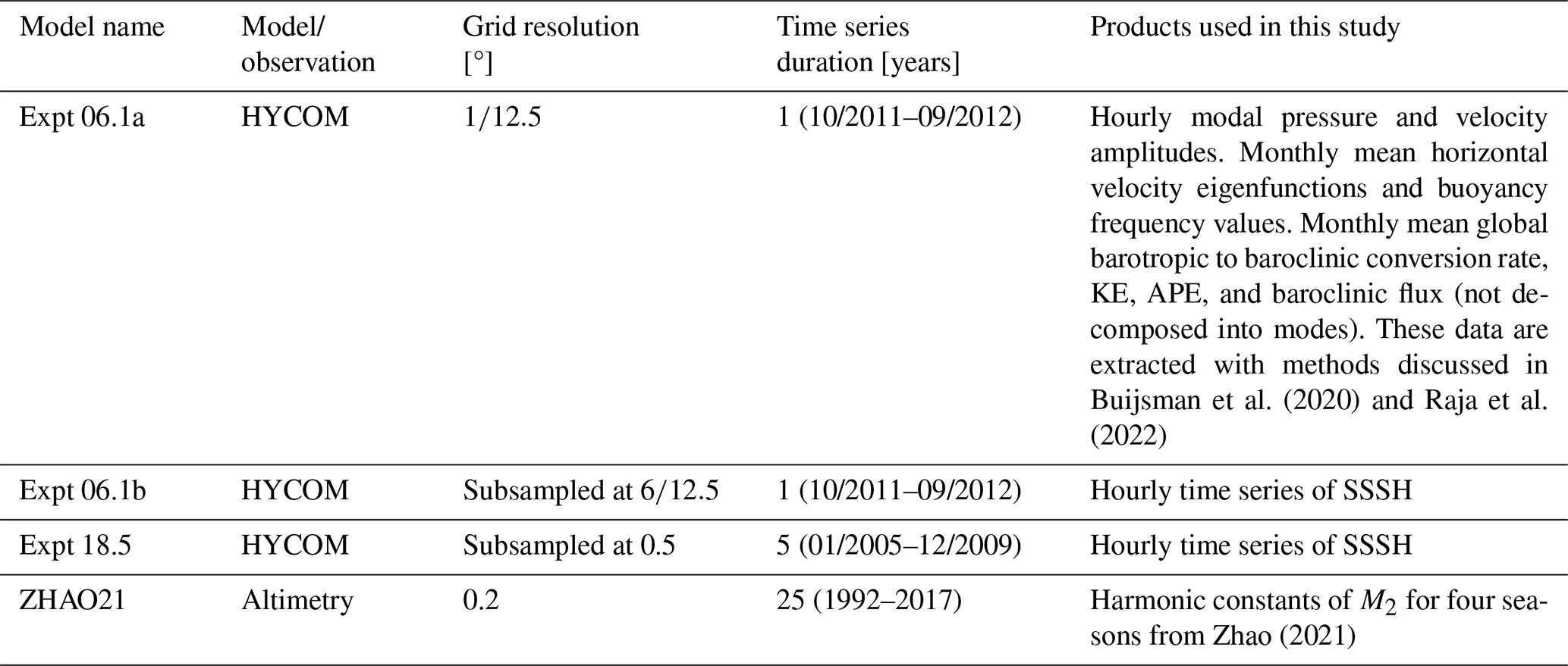

Table 1 List of datasets used in this study.

2.1.1 Expt 06.1

For expt 06.1, the data are available for 1 year, from October 2011 to September 2012. We use SSSH and internal tide energy terms from this simulation. This non-data assimilative simulation is forced with realistic atmospheric and tidal forcing (M₂, S₂, N₂, K₁, O₁). This simulation uses realistic atmospheric forcing from the NAVY Global Environmental Model (NAVGEM) (Hogan et al., 2014). The horizontal resolution is 8 km with 41 vertical layers. In expt 06.1, an augmented state ensemble Kalman filter (ASEnKF) technique (Ngodock et al., 2016) is applied to improve the accuracy of barotropic tides. A parameterized topographic wave drag (Jayne and St. Laurent, 2001) and a scalar self-attraction and loading correction (SAL; Hendershott, 1972; Ray, 1998) are used. The spin-up time of the background circulation and tides for this model simulation is 15 years and 2 months, respectively (Buijsman et al., 2017). For more details on this simulation, the reader is referred to Buijsman et al. (2017) and Buijsman et al. (2020).

We use hourly SSSH snapshots subsampled at $\mathrm{6}/\mathrm{12.5}$° to analyze the seasonal variability in the semidiurnal internal tide SSSH. We refer to this time series as “expt 06.1b” (Table 1). The monthly mean and depth-integrated semidiurnal barotropic to baroclinic conversion rate, KE, APE, and baroclinic flux fields (not decomposed into modes) are computed by reconstructing harmonic time series for the sum of the M₂, S₂, and N₂ constituents. The global mean SSSH amplitude ratio of $M_{\mathrm{2}}:S_{\mathrm{2}}:N_{\mathrm{2}}$ is $\mathrm{1.0}:\mathrm{0.44}:\mathrm{0.30}$. In addition, the modal pressure and baroclinic velocity amplitudes as well as the horizontal velocity eigenfunctions are used to calculate mode 1 baroclinic (BC) SSH and energy terms. We refer to these data as “expt 06.1a” (Table 1).

2.1.2 Expt 18.5

We also use 5-year-long datasets from a global HYCOM simulation with a horizontal resolution of 8 km and 32 vertical layers to analyze the seasonal variability. This simulation features realistic atmospheric and tidal forcing. It is forced with four semidiurnal constituents (M₂, S₂, N₂, and K₂) and four diurnal constituents (K₁, O₁, P₁, and Q₁). This simulation is run from 2003 to 2011 with the atmospheric forcing from the Navy Operational Global Atmospheric Prediction System (NOGAPS) (Rosmond et al., 2002). A parameterized topographic wave drag (Arbic et al., 2010) and a scalar self-attraction and loading correction (SAL; Hendershott, 1972; Ray, 1998) are used. The spin-up time of the background circulation and tides for this model simulation is 13 years and 13 months, respectively (Metzger et al., 2010; Buijsman et al., 2016). For more details on this simulation, the reader is referred to Shriver et al. (2012), Buijsman et al. (2016), and Nelson et al. (2019).

To analyze the seasonal cycle in the semidiurnal internal tide SSSH, we use SSSH snapshots that are saved once per hour from 1 January 2005 to 31 December 2009. These snapshots are subsampled at 0.5° grid resolution.

2.2 Methodology

2.2.1 Seasonal variability in steric sea surface height

We analyze the seasonal variability in the semidiurnal SSSH. Steric SSH is calculated in real time as part of the HYCOM simulation (Savage et al., 2017). Although it has been shown in Zaron and Ray (2023) and Kaur (2024) that the semidiurnal internal tide amplitude of SSSH is larger than the true semidiurnal internal tide SSH amplitude by about 20 %, Kaur (2024) shows that the spatiotemporal variability is the same for the semidiurnal SSSH and the true semidiurnal internal tide SSH. We use harmonic analysis to extract the M₂, S₂, and N₂ constituents, from which we calculate the semidiurnal signal. To extract the semidiurnal signal, we prefer harmonic analysis over bandpass analysis because the latter method also captures some mesoscale variance, particularly at higher latitudes (results not shown), and numerical noise (thermobaric instability; Buijsman et al., 2020).

We extract monthly M₂, S₂, and N₂ amplitudes using the 5-year hourly time series of SSSH from expt 18.5. Using a least-squares fit analysis, we compute the harmonic constants of the M₂, S₂, N₂, K₁, and O₁ constituents for each month (730 h). The duration of 730 h is long enough to resolve these five constituents. However, there is a possibility of tidal aliasing due to K₂ and P₁. This is because both K₂ and S₂ and K₁ and P₁ are separated by two cycles per year. It is important to note that this tidal aliasing only affects the semiannual signal for S₂ and not the annual signal (results not shown). The SSSH time series of the M₂, S₂, and N₂ internal tide can be written as

$$\begin{array}{}\text{(1)}& \mathit{\eta }(t{)}_m=\sum _j{a}_j(m)\cos \left({\mathit{\omega }}_{j}t\right)+b_j(m)\sin \left({\mathit{\omega }}_{j}t\right),\end{array}$$

where t is time; m is the index for each month; a and b are harmonic constants for the month; j refers to the M₂, S₂, and N₂ constituents; and ω is the frequency. The semidiurnal SSSH variance for each month is calculated as

$$\begin{array}{}\text{(2)}& {\mathit{\sigma }}_{D\mathrm{2}}^{\mathrm{2}}\left(m\right)={\displaystyle \frac{\mathrm{1}}{T}}\int {\left({\mathit{\eta }}_m\right)}^{\mathrm{2}}\mathrm{d}t,\end{array}$$

where T is the number of hours in each month.

To calculate the seasonal variability in the semidiurnal internal tide SSSH variance, the annual cycle is fitted to the 5-year time series of the monthly semidiurnal SSSH variance (${\mathit{\sigma }}_{D\mathrm{2}}^{\mathrm{2}}$) with a least-squares method after removing the linear trend

$$\begin{array}{}\text{(3)}& {\widehat{\mathit{\sigma }}}_{D\mathrm{2}}^{\mathrm{2}}\left(m\right)=A_{\mathrm{a}}\cos \left({\mathit{\omega }}_{\mathrm{a}}{t}_m-{\mathit{\varphi }}_{\mathrm{a}}\right),\end{array}$$

where ω_a is the annual frequency; A_a and ϕ_a are the amplitude and phase of the annual signal, respectively; ${\widehat{\mathit{\sigma }}}_{D\mathrm{2}}^{\mathrm{2}}$ is the fitted time series; t_m=30.42m; and each month has 30.42 d.

We calculate the coefficient of determination (R²) for the annual fit of the time series of the monthly variance. It identifies how much of the variability in the semidiurnal SSSH variance is due to the seasonality. The coefficient of determination for the fit is given by

$$\begin{array}{}\text{(4)}& R^{\mathrm{2}}=\mathrm{1}-{\displaystyle \frac{{\sum }_{m=\mathrm{1}}^M\left[{\mathit{\sigma }}_{D\mathrm{2}}^{\mathrm{2}\prime }\right(m)-{\widehat{\mathit{\sigma }}}_{D\mathrm{2}}^{\mathrm{2}}(m){]}^{\mathrm{2}}}{{\sum }_{m=\mathrm{1}}^M\left[{\mathit{\sigma }}_{D\mathrm{2}}^{\mathrm{2}\prime }\right(m){]}^{\mathrm{2}}}},\end{array}$$

where ${\mathit{\sigma }}_{D\mathrm{2}}^{\mathrm{2}\prime }\left(m\right)$ is the detrended time series of the monthly semidiurnal variance and M is the total number of months.

2.2.2 Internal tide energetics

We analyze the seasonal variability in the semidiurnal internal tide energetics and compare it with the SSSH variance. Following Buijsman et al. (2017), we compute the monthly mean and depth-integrated semidiurnal barotropic to baroclinic energy conversion rate, KE, APE, and baroclinic energy flux from hourly 3D data of expt 06.1a. Initially, two sets of energy terms are computed for each month. For the first set, we bandpass the monthly time series of the 3D fields between 9 and 15 h, compute the energy terms every hour, remove the first and last 24 h to mitigate the effects of ringing, and finally average over time to compute the time-mean energy terms. For the second set, we bandpass the time series of the 3D fields between 9 and 15 h; extract the harmonic constants for the M₂, S₂, and N₂ constituents; reconstruct the harmonic time series; compute the energy terms every hour; remove the first and last 24 h to mitigate the effects of ringing; and finally average over time to compute the time-mean energy terms. The order of most steps is similar for both sets, which allows us to compare the total (bandpassed) internal tide energetics of the first set with the phase-locked internal tide energetics of the second set (Buijsman et al., 2017). However, at high latitudes, mesoscale motions and numerical noise adulterate the energetics of the first set. Hence, we use the second set based on the harmonic time series in this paper.

The depth-integrated and time-averaged internal tide energy balance equation is written as (Buijsman et al., 2016; Kang and Fringer, 2012)

$$\begin{array}{}\text{(5)}& \langle C\rangle =\langle {\displaystyle \frac{\partial E}{\partial t}}\rangle +\langle {\mathrm{\nabla }}_h\cdot \mathit{F}\rangle +\mathcal{R},\end{array}$$

where 〈〉 indicates the time average over a month; C is the depth-integrated barotropic to baroclinic conversion; E is the depth-integrated total baroclinic wave energy; ∇_h⋅F is the horizontal divergence of the depth-integrated baroclinic energy flux $\mathit{F}=(F_x,F_y)$; ℛ is the residual, which is mostly due to baroclinic energy dissipation; and $\frac{\partial E}{\partial t}$ is the tendency term. For periodic internal waves in the open ocean, the energy tendency is about 0 when averaged over multiple tidal cycles (Buijsman et al., 2016, 2020).

The depth-integrated and time-averaged conversion of baroclinic tides from barotropic tides for each x, y coordinate is

$$\begin{array}{}\text{(6)}& \langle C\rangle ={\displaystyle \frac{\mathrm{1}}{T}}\underset{\mathrm{0}}{\overset{T}{\int }}W(z=-H,t)p^{\prime }(z=-H,t)\mathrm{d}t,\end{array}$$

where $W(z=-H,t)$ is the vertical barotropic velocity at the sea floor, $p^{\prime }(z=-H,t)$ is the perturbation pressure at the sea floor, z is the vertical coordinate, and H is the water depth. The perturbation pressure is calculated as in Nash et al. (2005) and by removing the depth mean pressure. The vertical barotropic velocity at the sea floor for each x, y coordinate is given by

$$\begin{array}{}\text{(7)}& W(z=-H,t)=-\mathit{U}\left(t\right)\cdot {\mathrm{\nabla }}_{h}H,\end{array}$$

where $\mathit{U}=(U,V)$ are the barotropic velocities in the x and y directions. The depth-integrated and time-averaged baroclinic flux for each x, y coordinate is calculated as

$$\begin{array}{}\text{(8)}& \langle \mathit{F}\rangle ={\displaystyle \frac{\mathrm{1}}{T}}\underset{\mathrm{0}}{\overset{T}{\int }}\underset{-H}{\overset{\mathrm{0}}{\int }}{\mathit{u}}^{\prime }(z,t)p^{\prime }(z,t)\mathrm{d}z\mathrm{d}t,\end{array}$$

where ${\mathit{u}}^{\prime }=(u^{\prime }$, v^′) are the horizontal baroclinic velocities in the x and y directions. The depth-integrated and time-averaged KE for each x, y coordinate is calculated as

$$\begin{array}{}\text{(9)}& \langle KE\rangle ={\displaystyle \frac{\mathrm{1}}{T}}\underset{\mathrm{0}}{\overset{T}{\int }}\underset{-H}{\overset{\mathrm{0}}{\int }}{\displaystyle \frac{\mathrm{1}}{\mathrm{2}}}{\mathit{\rho }}_{\mathrm{0}}\left(u^{\prime }\right(z,t{)}^{\mathrm{2}}+v^{\prime }(z,t{)}^{\mathrm{2}})\mathrm{d}z\mathrm{d}t,\end{array}$$

where ρ₀ is the reference density. The depth-integrated and time-averaged APE for each x, y coordinate is calculated as

$$\begin{array}{}\text{(10)}& \langle \mathrm{APE}\rangle ={\displaystyle \frac{\mathrm{1}}{T}}\underset{\mathrm{0}}{\overset{T}{\int }}\underset{-H}{\overset{\mathrm{0}}{\int }}{\displaystyle \frac{g^{\mathrm{2}}{\mathit{\rho }}^{\prime }(z,t{)}^{\mathrm{2}}}{\mathrm{2}{\mathit{\rho }}_{\mathrm{0}}{N}^{\mathrm{2}}(z,t)}}\mathrm{d}z\mathrm{d}t,\end{array}$$

where g is the gravitational acceleration, N is the buoyancy frequency, and ρ^′ is the perturbation density. The depth-integrated total baroclinic energy is the sum of depth-integrated KE and APE. The buoyancy frequency is calculated as

$$\begin{array}{}\text{(11)}& N^{\mathrm{2}}=-{\displaystyle \frac{g}{{\mathit{\rho }}_{\mathrm{0}}}}{\displaystyle \frac{\partial \langle \mathit{\rho }\rangle }{\partial z}},\end{array}$$

where 〈ρ〉 is the mean potential density and $\left(\frac{\partial \langle \mathit{\rho }\rangle }{\partial z}\right)$ is the vertical density gradient. In the remainder of the paper, we will drop the 〈〉 when discussing the time-averaged energy terms.

For expt 06.1, all variables (SSSH variance, barotropic to baroclinic conversion, KE, APE, total energy, and flux) are calculated for each month from October 2011 to September 2012. The exact number of hours per month is used. The hours for each month from October 2011 to September 2012 are as follows: 744, 720, 744, 744, 696, 744, 720, 744, 720, 744, 383, and 889. For August, we use the first 2 weeks of data because the model data for the third week were corrupted in storage. We add the last week of August to September, resulting in 5 weeks of data for September. However, the short months, February and August, show outlier values. The 14 d of August are not sufficient to resolve the M₂, S₂, and N₂ constituents because M₂ has a beat period of 27.55 d with N₂. While February has 29 d, the mean is computed over 27 d because the tail ends of the time series are omitted. We believe that these 2 missing days may have impacted the energy values for the month of February globally. Therefore, we remove the monthly mean values for February and August for each grid point and then linearly interpolate the values for these 2 months using data from adjacent months. The SSSH variance values are subsampled at $\mathrm{6}/\mathrm{12.5}$° resolution. Hence, we also subsample KE, APE, total energy, and flux at $\mathrm{6}/\mathrm{12.5}$° resolution.

2.2.3 Modal energetics

We decompose internal tide SSH and energetics into vertical modes to better understand the discrepancies in seasonal trends between SSSH variance and energy terms. For the calculation of mode 1 baroclinic SSH, KE, and APE, 3D HYCOM fields from expt 06.1a are decomposed into vertical modes following Buijsman et al. (2020) and Raja et al. (2022). The eigenfunctions of the first five modes are computed for each month by solving the Stürm–Liouville equation using the monthly mean and spatially varying buoyancy frequency (Gerkema and Zimmerman, 2008). The horizontal velocity eigenfunctions are projected onto the perturbation pressure and baroclinic velocity time series to obtain a modal amplitude time series for pressure and velocities.

To compare with SSSH, we compute the mode 1 SSH. For each x, y coordinate the following applies:

$$\begin{array}{}\text{(12)}& p_{\mathrm{1}}(z,t)={\stackrel{\mathrm{̃}}{p}}_{\mathrm{1}}\left(t\right){\mathcal{U}}_{\mathrm{1}}\left(z\right),\end{array}$$

where p₁ is the mode 1 pressure, ${\stackrel{\mathrm{̃}}{p}}_{\mathrm{1}}\left(t\right)$ is the mode 1 amplitude time series of pressure, and 𝒰₁(z) is the horizontal velocity eigenfunction of mode 1. The mode 1 SSH is calculated as

$$\begin{array}{}\text{(13)}& {\mathit{\eta }}_{\mathrm{1}}\left(t\right)={\displaystyle \frac{p_{\mathrm{1}}(z=\mathrm{0},t)}{g{\mathit{\rho }}_{\mathrm{0}}}}.\end{array}$$

We extract the harmonic constants for the M₂, S₂, and N₂ internal tide from the hourly time series of mode 1 SSH and bottom perturbation pressure ($p_{\mathrm{1}}(z=-H,t)$) for each month. Then, the variance for semidiurnal mode 1 SSH and bottom perturbation pressure is calculated using Eqs. (1) and (2).

For calculation of the mode 1 semidiurnal KE and APE, we extract the harmonic constants for M₂, S₂, and N₂ constituents for each month from the time series of the mode 1 amplitudes of baroclinic velocities and pressure. The mode 1 semidiurnal KE and APE are calculated as (Kelly et al., 2012)

$$\begin{array}{}\text{(14)}& {\displaystyle }K{E}_{\mathrm{1}}=\sum _j\left(|{\widehat{u}}_{\mathrm{1}j}{|}^{\mathrm{2}}+|{\widehat{v}}_{\mathrm{1}j}{|}^{\mathrm{2}}\right){\displaystyle \frac{H{\mathit{\rho }}_{\mathrm{0}}}{\mathrm{4}}},\text{(15)}& {\displaystyle }AP{E}_{\mathrm{1}}=\sum _j\left(\mathrm{1}-{\displaystyle \frac{f^{\mathrm{2}}}{{\mathit{\omega }}_j^{\mathrm{2}}}}\right){\displaystyle \frac{|{\widehat{p}}_{\mathrm{1}j}{|}^{\mathrm{2}}}{c_{\mathrm{1}}^{\mathrm{2}}{\mathit{\rho }}_{\mathrm{0}}}}{\displaystyle \frac{H}{\mathrm{4}}},\end{array}$$

where ${\widehat{u}}_{\mathrm{1}j}$, ${\widehat{v}}_{\mathrm{1}j}$, and ${\widehat{p}}_{\mathrm{1}j}$ are the mode 1 complex harmonic constants of the baroclinic velocities and perturbation pressure for constituent j; c₁ is the mode 1 eigenspeed; and f is the Coriolis frequency.

The mode 1 variables are also linearly interpolated for February and August for each grid point using the same methodology as we employed for the undecomposed fields. Additionally, we subsample these variables at $\mathrm{6}/\mathrm{12.5}$° resolution to compare with the SSSH variance.

2.2.4 Satellite altimeter data

We validate the seasonal variability in the HYCOM mode 1 M₂ baroclinic SSH variance and KE with the satellite altimeter data of Zhao (2021). Zhao (2021) analyzed the seasonal variability in the mode 1 M₂ internal tide using 25 years of multisatellite altimeter data from 1992 to 2017. Zhao (2021) could only extract mode 1 M₂ amplitudes with reasonable accuracy for four seasons: winter (January, February, and March), spring (April, May, and June), summer (July, August, and September), and fall (October, November, and December). Thus, the satellite observations may underestimate the amplitudes of the seasonal variability. The variance for each season is calculated as

$$\begin{array}{}\text{(16)}& {\mathit{\sigma }}_s^{\mathrm{2}}={\displaystyle \frac{{A_s}^{\mathrm{2}}}{\mathrm{2}}},\end{array}$$

where A_s is the mode 1 M₂ internal tide SSH amplitude for season s.

3 Results

3.1 Spatial variability in SSSH and energy

The mean values over 12 months for semidiurnal SSSH variance, depth-integrated semidiurnal barotropic to baroclinic conversion rate, depth-integrated semidiurnal baroclinic energy, and depth-integrated semidiurnal baroclinic flux for expt 06.1 are shown in Fig. 1. The baroclinic energy and flux values are subsampled at $\mathrm{6}/\mathrm{12.5}$° to compare with the SSSH variance.

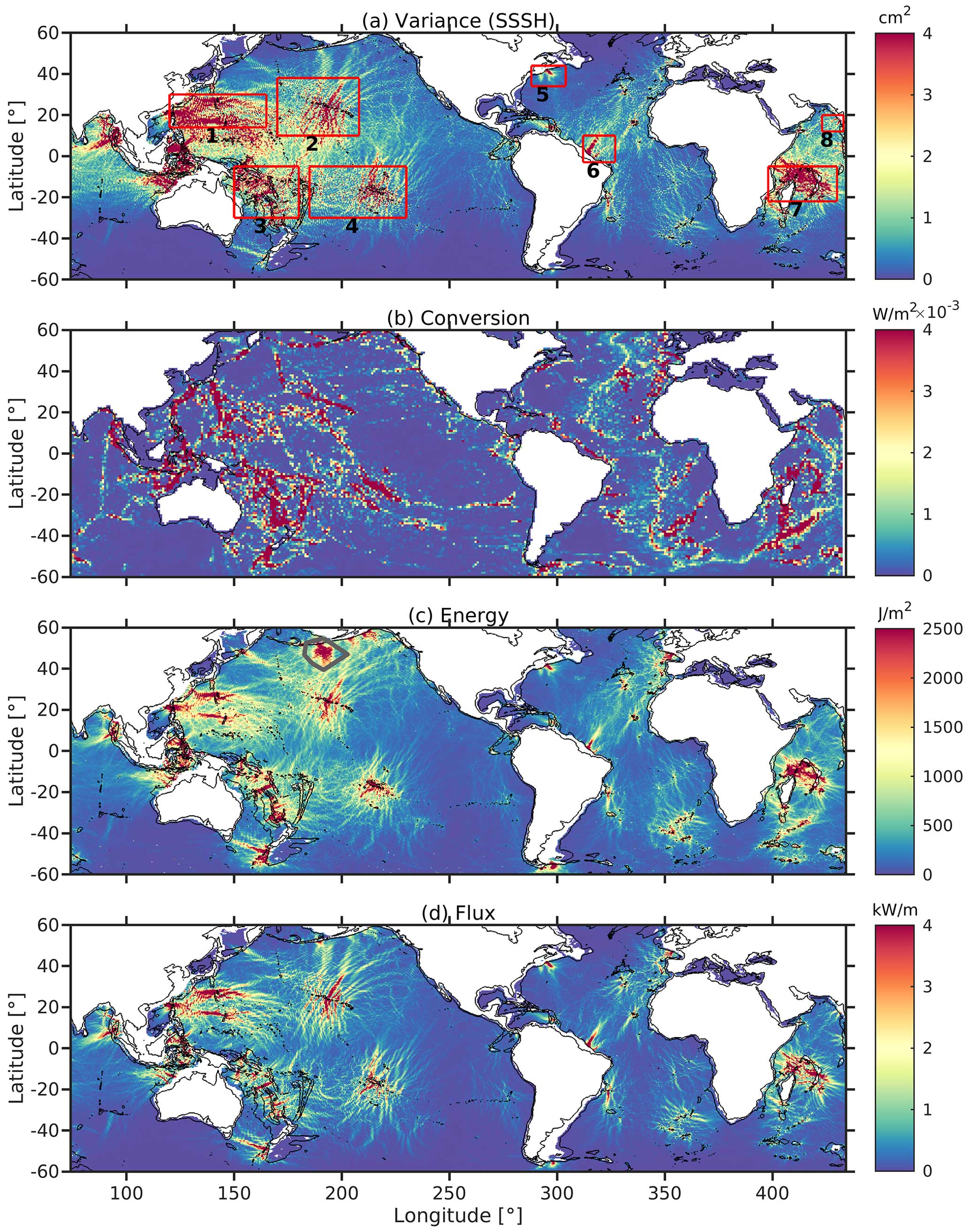
Figure 1 (a) Monthly semidiurnal SSSH variance, (b) depth-integrated semidiurnal barotropic to baroclinic conversion rate, (c) baroclinic semidiurnal energy, and (d) baroclinic semidiurnal flux of expt 06.1 averaged over 12 months. In (a), (c), and (d), black bathymetry contours are plotted at 0 m and 2000 m. In (a), the following regions are marked: (1) east of Philippines, (2) Hawaii, (3) tropical SW Pacific, (4) tropical South Pacific, (5) Georges Bank, (6) Amazon Plume, (7) Madagascar, and (8) Arabian Sea. In (b), conversion rates are area-averaged to 1° grid resolution, and black bathymetry contours are plotted at 0 m. In (c), the gray polygon marks the area affected by thermobaric instabilities.

The barotropic to baroclinic conversion rate in Fig. 1b is higher at ridges and rough topography, highlighting the internal tide generation sites. SSSH variance, energy, and flux values are also higher near the generation sites (Fig. 1). The patterns for APE and KE (not shown) are the same as total energy (Fig. 1c). The polygon in Fig. 1c marks an area in the North Pacific with elevated KE, which may be attributed to thermobaric instability (TBI). TBI is a numerical instability present in Lagrangian/isopycnic vertical coordinate ocean models due to inaccurate compensation for compressibility in calculating pressure gradient accelerations (Hallberg, 2005). TBI is known to occur in the North Pacific Ocean in both expt 06.1 and expt 18.5 (Buijsman et al., 2016, 2020). Although TBI is a broadband signal with a variable phase, it is possible that some of this noise projects on the harmonic constants. We omit the area with TBI because it adversely impacts the seasonal variability analysis.

3.2 Seasonal variability in steric sea surface height

The first objective is to analyze the seasonal variability in semidiurnal internal tide SSSH variance. We use the detrended monthly variance (${\mathit{\sigma }}_{D\mathrm{2}}^{\mathrm{2}\prime }$) of the combined M₂, S₂, and N₂ internal tides, which is computed with hourly time series of SSSH from expt 18.5. We use expt 18.5 because this simulation has a 5-year duration, which benefits the calculation of the annual seasonal cycle. Using a least-squares fit analysis, we calculate the annual cycle of the monthly variance in semidiurnal internal tide SSSH. The amplitude of the annual cycle is normalized by the mean semidiurnal variance over 60 months (Fig. 2a). We use the normalized amplitude (Fig. 2a) and R² (Fig. 2c) as indicators of the seasonal variability. If the normalized amplitude is small, there is not much seasonal variability in SSSH variance. Hence, we focus on areas where both the normalized amplitude and R² are significant.

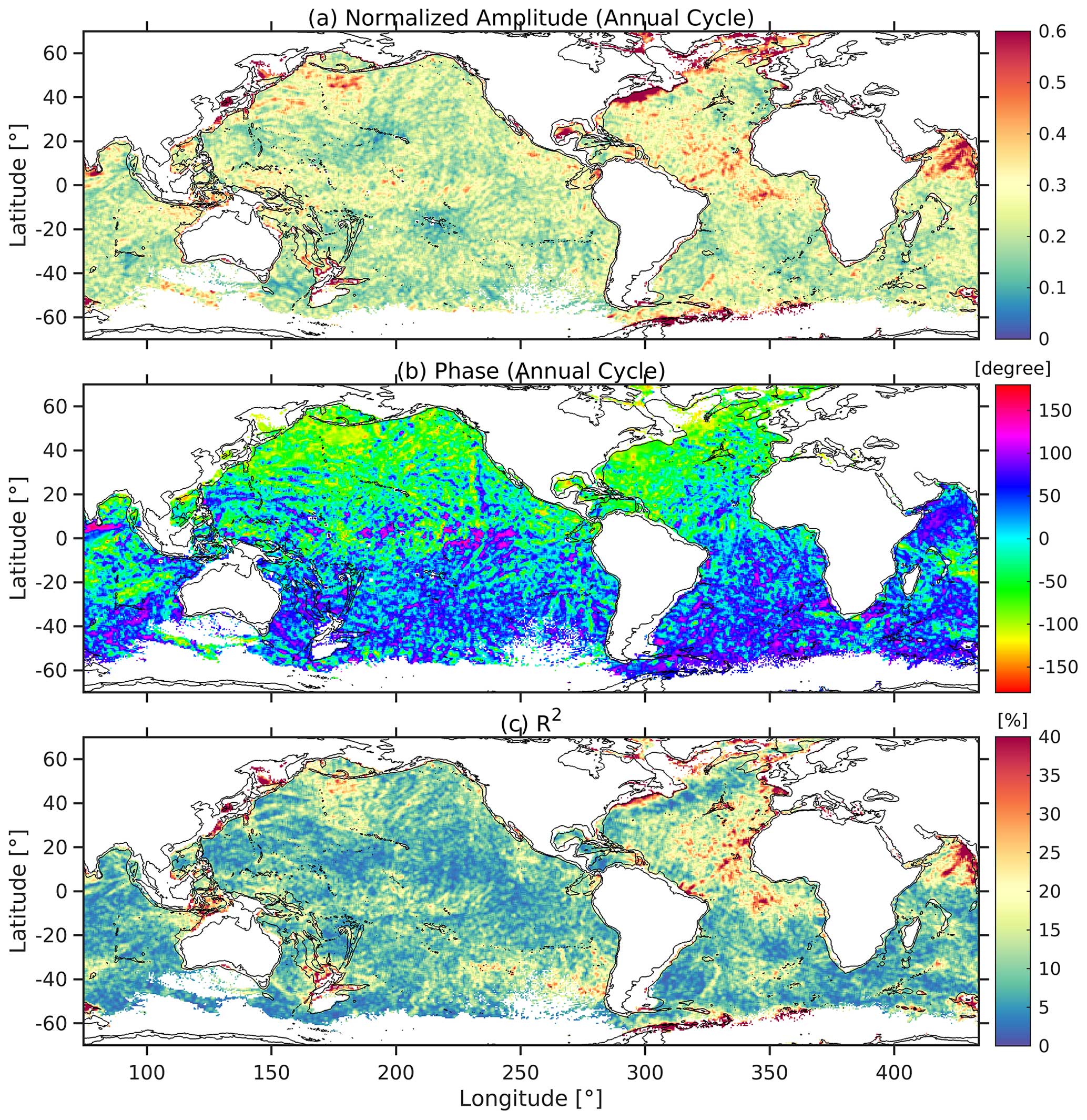
Figure 2 (a) The normalized amplitude and (b) phase of the annual cycle of the monthly semidiurnal SSSH variance (${\mathit{\sigma }}_{D\mathrm{2}}^{\mathrm{2}\prime }$). (c) The coefficient of determination (R²) for the fit. Black bathymetry contours are plotted at 0 and 2000 m. The normalized amplitude, phase, and R² are computed for each point and smoothed by taking a nine-point (3×3 square box) running mean. The areas with small internal tides (mean monthly variance < 0.01 cm²) are removed. Data are from expt 18.5.

The internal tides generated in the coastal areas of Georges Bank and the Arabian Sea display the largest seasonal variability (Fig. 2a and c). Figure 2b shows that the seasonal cycle of the semidiurnal internal tide SSSH variance in the Northern Hemisphere is 180° out of phase with the variance in the Southern Hemisphere. If the phase is 90° (−90°), the semidiurnal SSSH variance is maximum in April (October), which implies internal tides are stronger in respective fall months in the Northern Hemisphere and Southern Hemisphere. This suggests that seasonal changes in the semidiurnal SSSH variance may be due to stratification, which can affect the propagation and/or generation of the internal tides. In the next section, we investigate whether the same seasonal variability is present in the internal tide energetics.

3.3 Seasonal variability in internal tide energetics

In this section, we analyze the seasonal trend in semidiurnal internal tide energetics and compare it with the seasonal trend in semidiurnal SSSH variance. To do so, we use 1-year data from expt 06.1 to calculate the monthly semidiurnal SSSH variance, depth-integrated conversion rate, KE, APE, energy, and flux for M₂, S₂, and N₂ constituents. Unfortunately, the annual cycle fit similar to Fig. 2 for the internal tide energetics is very noisy because 1 year of data is insufficient to fit the annual signal accurately. Hence, we do not show these results.

To better visualize the seasonal trends, we zonally average the conversion rate, flux, SSSH variance, KE, APE, and total energy over 10° latitude bins for the Atlantic and the Pacific oceans for each 1-month period. The values in areas shallower than 100 m are excluded from the analysis because the model does not resolve internal tides satisfactorily in these areas. To derive the anomaly time series for these variables, we remove and normalize by their annual mean values. The anomaly plots are presented in Figs. 3 and 4 for the Pacific and Atlantic oceans, respectively. In Appendix A, we calculate the zonally averaged SSSH variance anomaly time series from expt 18.5 for all 5 years, following a similar approach to that for expt 06.1. Our findings indicate that the seasonal variability in expt 18.5 closely resembles that of expt 06.1. Hence, we use this method to analyze the seasonal variability in expt 06.1.

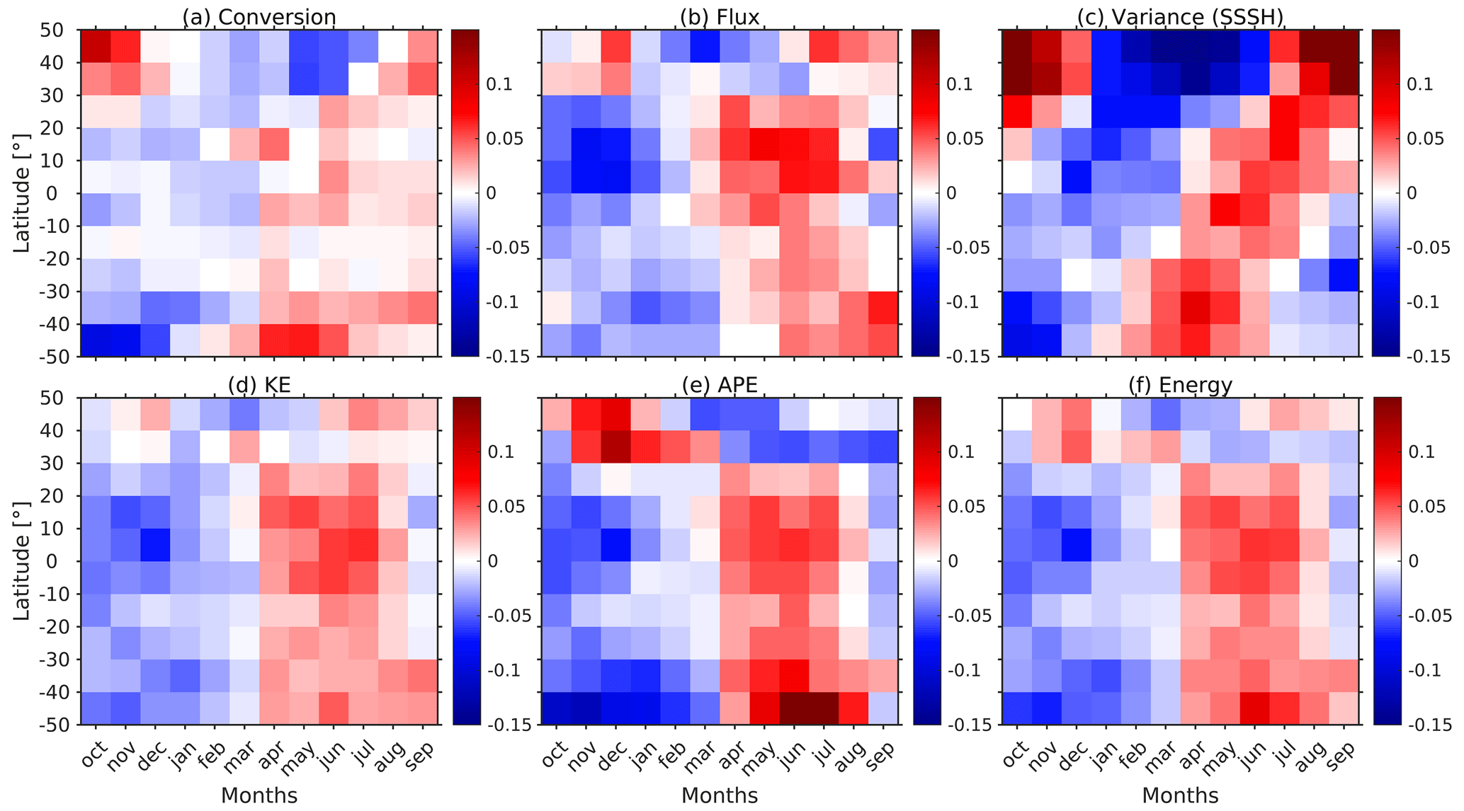
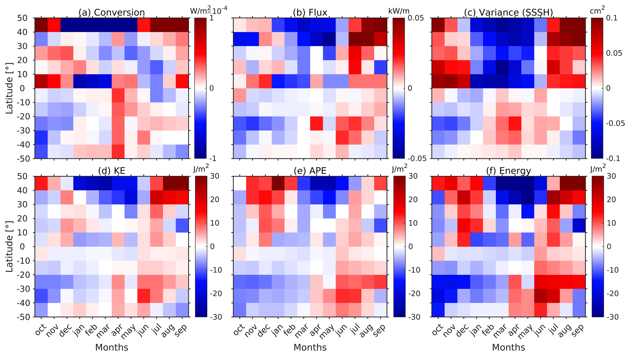
Figure 3 Zonally averaged anomaly time series of monthly semidiurnal (a) barotropic to baroclinic conversion rate, (b) baroclinic energy flux, (c) SSSH variance, (d) KE, (e) APE, and (f) total energy for the Pacific Ocean. The anomalies are computed by removing and normalizing by the annual mean values. Data are from expt 06.1.

Figure 4 The same as Fig. 3, but for the Atlantic Ocean.

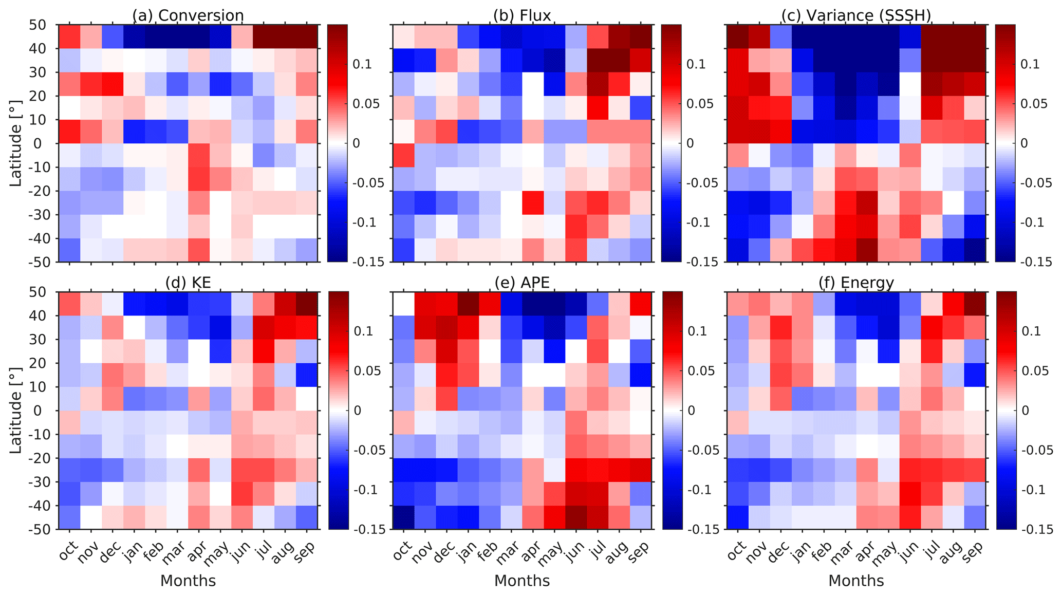
A seasonal cycle is observed in all variables (conversion rate, flux, SSSH variance, KE, APE, and total energy) in both the Pacific and Atlantic oceans (Figs. 3 and 4). While the seasonal trends are broadly similar for the energy terms in both oceans, they differ from the trends in the SSSH variance. Similar to Fig. 2b, the seasonal cycle of the SSSH variance is out of phase in the Northern Hemisphere and Southern Hemisphere in Figs. 3 and 4. By contrast, the energy terms do not follow the same trends for the two hemispheres. The seasonal cycles of the energy terms are out of phase with SSSH variance, and no apparent differences are present between the Northern Hemisphere and the Southern Hemisphere. However, both SSSH and energetics tend to show the largest amplitudes at higher latitudes.

The amplitude of the seasonal cycles in Figs. 3 and 4 is maximally about 15 % of the annual mean value. The percentage change is higher for the SSSH variance as compared to the conversion rate and KE. The percentage change for APE is also larger than the conversion rate and KE at higher latitudes. For a free-propagating internal tide, $\frac{\mathrm{KE}}{\mathrm{APE}}=\frac{{\mathit{\omega }}^{\mathrm{2}}+f^{\mathrm{2}}}{{\mathit{\omega }}^{\mathrm{2}}-f^{\mathrm{2}}}$ (Alford and Zhao, 2007). As ω≈f at higher latitudes, APE tends to 0. Therefore, APE is small at higher latitudes, and the percentage change for APE is large. To determine that the normalization is not misrepresenting the seasonal signal, we show the non-normalized anomalies in Figs. B1 and B2 in Appendix B. These figures show that the seasonal trends remain consistent. However, there is a difference in the amplitude because if the internal tide signal is small (large), it can increase (decrease) the percentage change. Additionally, it is important to emphasize that this study focuses primarily on trends and percentage change; therefore, utilizing the normalized data is preferable.

In the Pacific Ocean, the seasonal signal for the SSSH variance in the tropical region, spanning −20 to 20°, is marginally out of phase when compared with the polar regions (Fig. 3c). In this region, the seasonal signal in the SSSH variance is in sync with the internal tide energetics. In the Atlantic Ocean (Fig. 4), the seasonal cycle for energy terms is noisier than in the Pacific Ocean. This may be because the internal tide generation is weaker in the Atlantic Ocean, with most of the generation happening at deep ridges. The strong seasonal signal in the conversion from 40 to 50° N in Fig. 4a (and B2a) is attributed to Georges Bank.

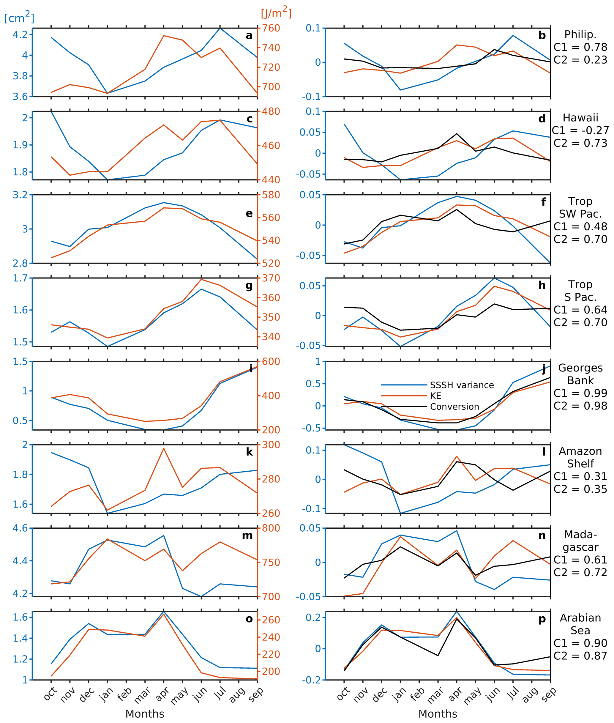
Figure 5 Area-averaged (left column) monthly semidiurnal SSSH variance (blue line) and KE (orange line) and (right column) normalized anomaly time series of monthly semidiurnal SSSH variance (blue line), KE (orange line), and conversion (black line) for regions marked by the red boxes in Fig. 1a. C1 and C2 are the correlation coefficients between SSSH variance and conversion and between KE and conversion, respectively. Data are from expt 06.1.

To further compare the seasonal signals, we plot in Fig. 5 the area-averaged semidiurnal SSSH variance, KE, and conversion anomalies for each month for eight regions (red boxes in Fig. 1a). The seasonal signal of KE and conversion is similar to that of the SSSH variance for Georges Bank and the Arabian Sea, where the strongest seasonal variability in internal tides is observed (Fig. 5i, j, o, and p). The strong seasonal variability in conversion rates in the Arabian Sea and Georges Bank and their relation to the stratification are further explained in Appendix C. The seasonal amplitudes of SSSH variance, KE, and conversion at Georges Bank and the Arabian Sea are ∼ 50 % and ∼ 20 %, respectively. This percentage is obtained from the normalized anomaly time series shown in the right column of Fig. 5. The correlation coefficient between SSSH variance and conversion at Georges Bank and the Arabian Sea is 0.99 and 0.90, respectively. However, for the tropical SW Pacific and the tropical South Pacific (Fig. 5e, f, g, and h), the seasonal signal of KE is similar to the SSSH variance but with a phase lag. For other regions, the discrepancies are more complex. Overall, the conversion shows a better correlation with KE than with SSSH variance, except east of the Philippines, where the correlation coefficient between KE and SSSH variance (0.78) is higher than between KE and conversion (0.23).

Our analysis indicates that the conversion rate is the primary factor responsible for the seasonal variability in internal tide energetics because the seasonal trends of conversion and other energy terms are similar. The amount of internal tide energy in the ocean is governed by the internal tide energy input over topography, which is computed with the conversion metric. However, the seasonal trends of SSSH variance are different from the trends in the energy terms, except for Georges Bank and the Arabian Sea, where the seasonal variability is the strongest. In Appendix C, we discuss the seasonal cycles in conversion for Georges Bank and the Arabian Sea and the environmental drivers in more detail. In the next section, we validate the seasonal variability in HYCOM with altimetry to ensure that the seasonal variability in HYCOM sea surface height is realistic. In the discussion section, we explain the observed differences in the seasonal variability between SSSH variance and internal tide energetics.

3.4 Comparison with the satellite altimeter data

To validate the seasonal variability in our model, we compare the mode 1 M₂ internal tide variance from the satellite altimeter data from Zhao (2021) for each season with the mode 1 M₂ SSH variance and mode 1 M₂ KE from the HYCOM simulation expt 06.1a in Fig. 6. It is discussed and shown later that semidiurnal mode 1 SSH variance and semidiurnal SSSH variance are in good agreement. To ensure accuracy, we omit areas with strong mesoscale activity from the satellite altimeter and HYCOM data. Additionally, we interpolate the mode 1 M₂ SSH variance and KE from the HYCOM simulation to the same locations as the altimetry data for each season. We then zonally average the M₂ variance from the satellite altimeter data, the M₂ baroclinic SSH variance, and the KE over 10° latitude bins for the Atlantic and the Pacific oceans for each season while also removing regions of weak internal tides (as in Zhao (2021), areas with M₂ internal tide SSH amplitude < 0.2 cm are removed). Finally, we remove and normalize by the annual mean.

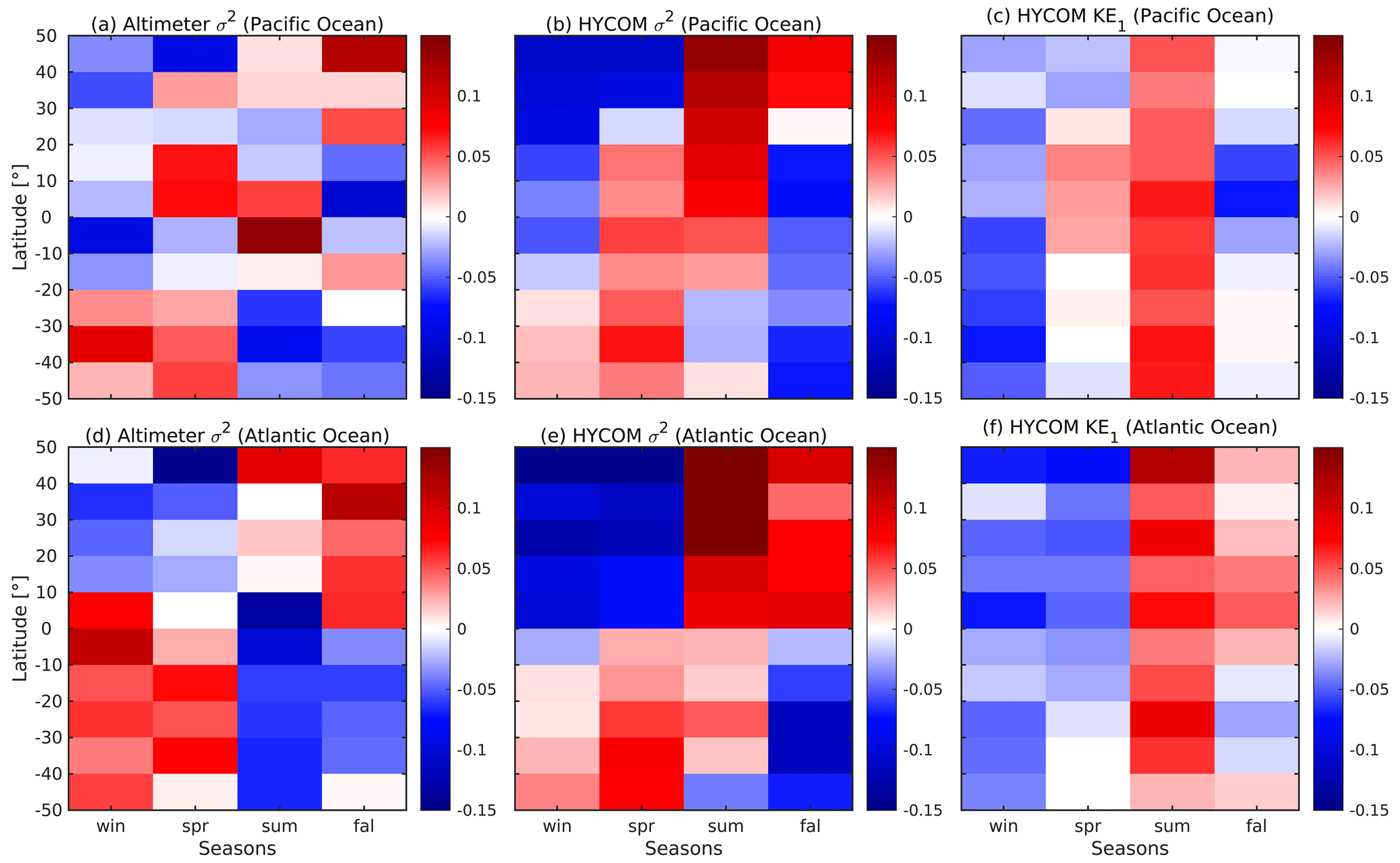
Figure 6 Zonally averaged normalized anomaly time series of seasonal mean mode 1 M₂ internal tide SSH variance for (a, d) the satellite altimeter data and (b, e) the HYCOM expt 06.1 data and (c, f) the mode 1 M₂ KE from HYCOM expt 06.1. The anomaly time series for the Pacific Ocean are in (a)–(c) and for the Atlantic Ocean they are in (d)–(f).

The seasonal variability in both HYCOM and satellite altimeter M₂ SSH variance for the Pacific and Atlantic oceans is in reasonable agreement. However, the level of agreement between the two is stronger in the Atlantic Ocean than in the Pacific Ocean. Moreover, the seasonal SSH variance in the satellite altimeter data is noisier than the HYCOM SSH variance. The reasons for this are not clear to us. It could be attributed to the sparseness of the satellite altimeter data in time and space. Despite these discrepancies, the trends observed in KE are different from both the HYCOM and satellite altimeter SSH variance, indicating that the seasonal variability in KE is different from the internal tide SSH variability. This comparison suggests that the trends in baroclinic SSH variance in HYCOM are realistic but that they do not reflect the seasonal variability in the internal tide energy except in Georges Bank and the Arabian Sea (Fig. 5).

4 Discussion

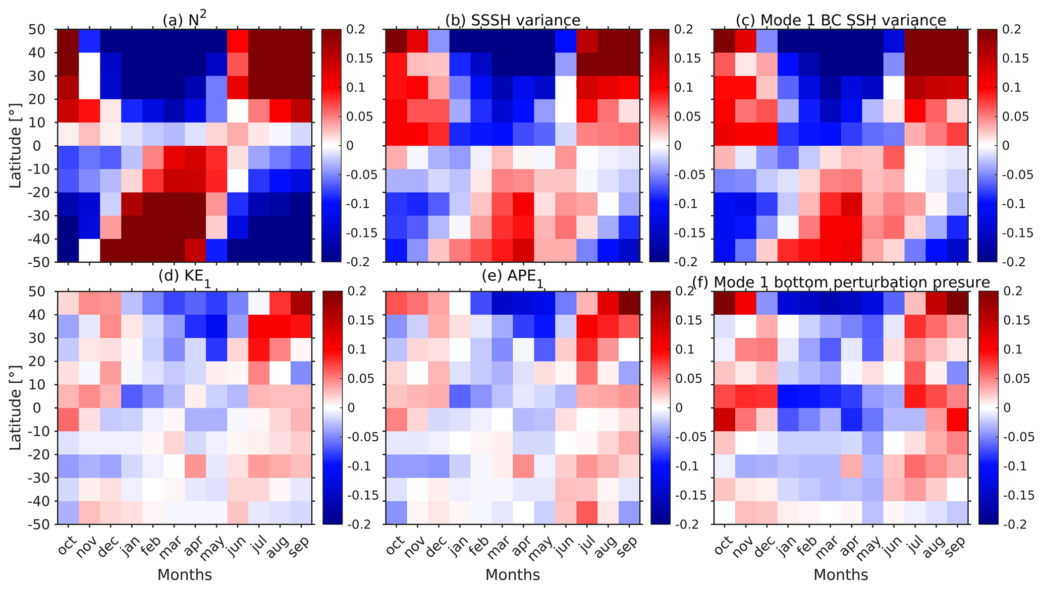
In this section, we explore the causes of the differences in the seasonal variability between SSSH variance and the energy terms. SSSH is strongly affected by the density of the surface layers, which varies significantly due to seasonal temperature changes (Qu and Melnichenko, 2023). Based on our analysis, the seasonal changes in semidiurnal SSSH variance may not accurately represent the actual seasonal changes in internal tide energy because the internal tide SSH may be modulated by changes in surface temperature. To understand this better, we compare the seasonal variability in SSSH variance with mode 1 SSH variance, KE, APE, bottom perturbation pressure variance, and depth mean buoyancy frequency.

We compute the mode 1 semidiurnal baroclinic SSH variance, bottom perturbation pressure variance, KE, and APE for each month using 3D fields from expt 06.1a. These variables are based on reconstructed time series for the M₂, S₂, and N₂ constituents. We consider mode 1 because the internal tide SSSH is dominated by mode 1 (Zhao et al., 2019; Buijsman et al., 2020). The spatial patterns of the time-mean bottom perturbation pressure variance are similar to the time-mean semidiurnal SSSH variance in Fig. 1a and are not shown.

We compare the seasonal trends in semidiurnal SSSH variance, mode 1 semidiurnal baroclinic SSH variance, KE, APE, bottom perturbation pressure variance, and N² for the Pacific and Atlantic oceans in Figs. 7 and 8. We zonally average these variables over 10° latitude bins for each basin and 1-month segment. For all variables, shallow areas are removed (depth < 100 m). To derive the anomaly time series, we remove and normalize by the annual mean values. We consider the seasonal variability in the bottom perturbation pressure variance to better understand the effect of surface stratification on the SSSH variance. As expected, the undecomposed SSSH variance and the mode 1 SSH variance have identical spatial and seasonal trends in Figs. 7b and c and 8b and c. By contrast, for both the Atlantic and Pacific oceans, the seasonal variability in bottom perturbation pressure variance resembles that of the energy terms and not that of the mode 1 SSH variance, which is based on the surface perturbation pressure. Interestingly, the seasonal trend in the depth mean buoyancy frequency is similar to the SSSH variance and mode 1 SSH variance, but it is 1–2 months ahead of the SSSH variance. The seasonal signal in the buoyancy frequency is out of phase in the Northern Hemisphere and Southern Hemisphere, which is similar to what we observe for the SSSH variance.

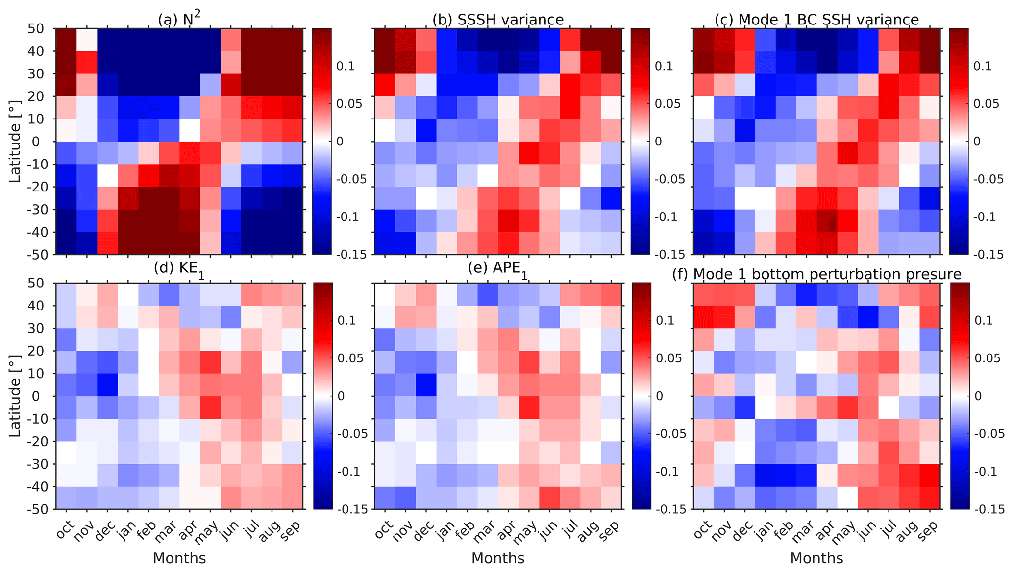
Figure 7 Zonally averaged normalized anomaly time series of monthly mean (a) depth mean N² and semidiurnal (b) undecomposed SSSH variance, (c) mode 1 SSH variance, (d) mode 1 KE, (e) mode 1 APE, and (f) mode 1 bottom perturbation pressure variance for the Pacific Ocean. The anomalies are computed by removing and normalizing by the annual mean values. Data are from expt 06.1.

Figure 8 The same as Fig. 7, but for the Atlantic Ocean.

The mode 1 SSH is computed as $\frac{\stackrel{\mathrm{̃}}{p_{\mathrm{1}}}\left(t\right){\mathcal{U}}_{\mathrm{1}}(z=\mathrm{0})}{g{\mathit{\rho }}_{\mathrm{0}}}$. To understand what is modulating the semidiurnal mode 1 SSH variance, we study the seasonal trend in mode 1 horizontal velocity eigenfunction at z=0 and the variance in the semidiurnal mode 1 perturbation pressure amplitude for the Pacific and Atlantic oceans (Fig. 9). The seasonal trends in ${\mathcal{U}}_{\mathrm{1}}^{\mathrm{2}}(z=\mathrm{0})$ are similar to the mode 1 SSH variance. The area-averaged correlation coefficient between the mode 1 SSH variance and ${\mathcal{U}}_{\mathrm{1}}^{\mathrm{2}}(z=\mathrm{0})$ is 0.84 and 0.89 for the Pacific and Atlantic oceans, respectively. Moreover, the seasonal variability in ${\mathcal{U}}_{\mathrm{1}}^{\mathrm{2}}(z=\mathrm{0})$ is similar to the depth-averaged buoyancy frequency anomaly in Figs. 7a and 8a. Specifically, when the buoyancy frequency is surface intensified at the end of summer, ${\mathcal{U}}_{\mathrm{1}}^{\mathrm{2}}$ is also surface intensified. Therefore, we conclude that the surface density stratification is the main factor that modulates the seasonal variability in semidiurnal SSSH variance. By contrast, the variance in the semidiurnal mode 1 perturbation pressure amplitude ($\stackrel{\mathrm{̃}}{p_{\mathrm{1}}}$) in Fig. 9c and f is more in agreement with the mode 1 KE and APE variability in Figs. 7 and 8. We note that 𝒰₁(z) does not contribute to the depth-integrated monthly values of mode 1 KE and APE because of the normalization condition ($\frac{\mathrm{1}}{H}{\int }_{-H}^{\mathrm{0}}{\mathcal{U}}_{\mathrm{1}}^{\mathrm{2}}\left(z\right)\mathrm{d}z=\mathrm{1}$; Buijsman et al., 2020). Hence, the seasonal effect due to stratification observed for surface values of 𝒰₁ disappears when depth-integrated.

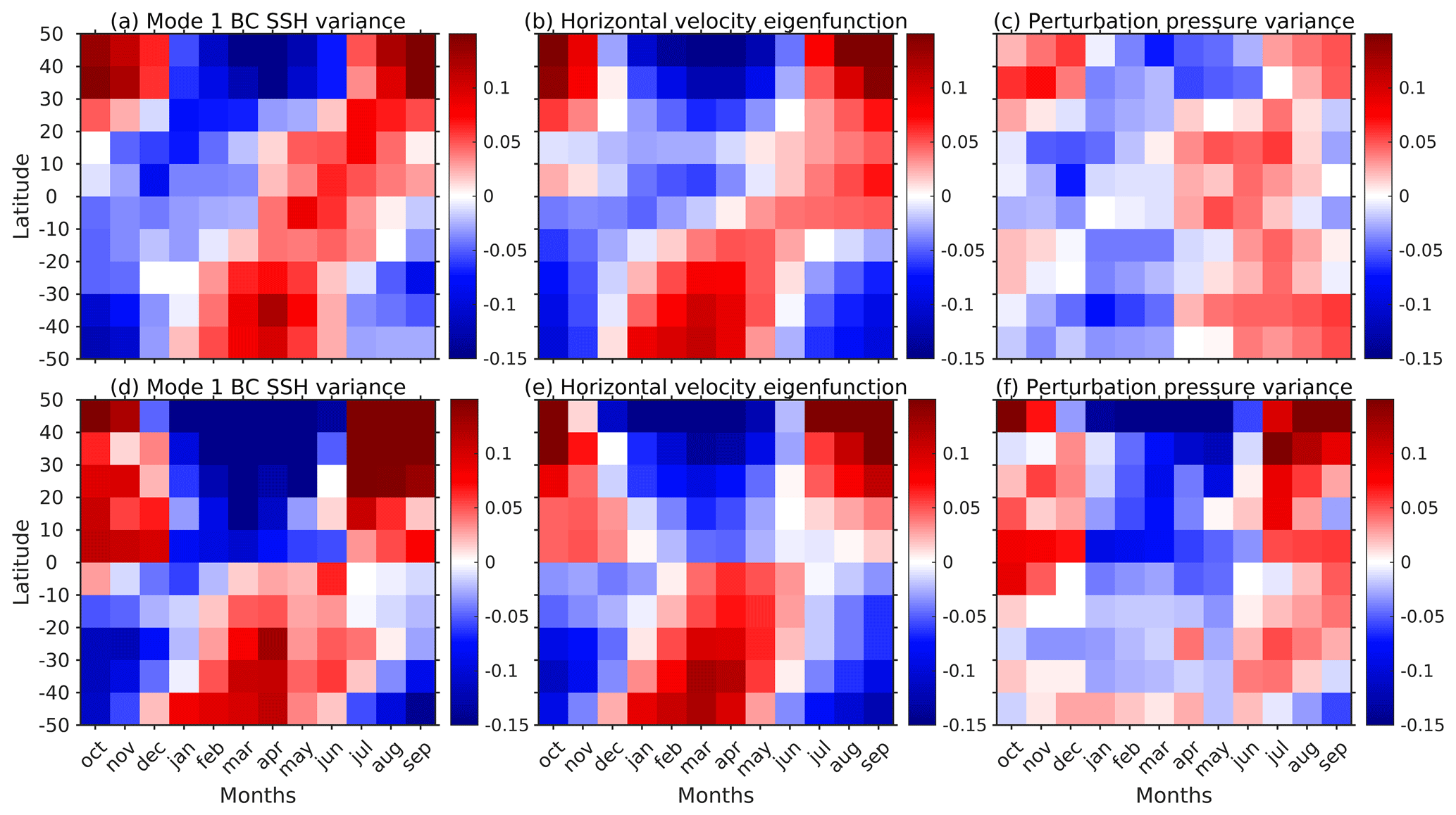
Figure 9 Zonally averaged normalized anomaly time series of (a, d) semidiurnal mode 1 baroclinic SSH variance, (b, e) mode 1 horizontal velocity eigenfunction (${\mathcal{U}}_{\mathrm{1}}^{\mathrm{2}}$) at z=0, and (c, f) semidiurnal mode 1 perturbation pressure amplitude ($\stackrel{\mathrm{̃}}{p_{\mathrm{1}}}$) variance for the Pacific Ocean (top row) and Atlantic Ocean (bottom row). Data are from expt 06.1.

Alternatively, we can also explain the modulation by considering APE. If we assume that the barotropic to baroclinic conversion rate remains constant throughout the year, we can assume that APE is constant. APE is proportional to $\frac{{\mathit{\rho }}^{\prime }(z,t{)}^{\mathrm{2}}}{N^{\mathrm{2}}(z,t)}$ (Eq. 10). If there is an increase (decrease) in surface temperature, N also increases (decreases), which means that ${\mathit{\rho }}^{\prime }(z,t)$ will also increase (decrease) for APE to remain constant. This increase (decrease) in ${\mathit{\rho }}^{\prime }(z,t)$ results in an increase (decrease) in SSSH.

5 Conclusions

In this study, we compare the seasonal variability in semidiurnal steric sea surface height (SSSH) with internal tide energetics, which are extracted from two non-data assimilative global Hybrid Coordinate Ocean Model (HYCOM) simulations. We analyze the seasonal trends in SSSH variance, barotropic to baroclinic conversion rate, kinetic energy (KE), available potential energy (APE), and pressure flux for semidiurnal internal tides. The seasonal variability in the HYCOM simulation is also compared with the satellite altimeter data of Zhao (2021).

The seasonal cycle of the semidiurnal SSSH variance is 180° out of phase in the Northern Hemisphere and Southern Hemisphere, which indicates that stratification may be responsible for this seasonal variability. We find that the amplitude of the seasonal cycles is about 10 %–15 % of the annual mean values when zonally averaged. The strongest seasonal variability in the semidiurnal SSSH variance is observed in Georges Bank and the Arabian Sea.

We compare the seasonal trend in semidiurnal SSSH variance with depth-integrated semidiurnal barotropic to baroclinic energy conversion rate, baroclinic energy flux, KE, and APE. The seasonal trends in the energy terms are quite similar. The conversion rate is dominant in influencing the seasonal variability in the internal tide energetics. However, we observe differences in the seasonal cycles between SSSH variance and the energy terms. Seasonal maxima in energy terms and SSSH do not coincide in space and time. Moreover, the seasonal cycles in the Northern Hemisphere and Southern Hemisphere are not clearly out of phase as for SSSH. The seasonal cycles of SSSH variance and the energy terms are only in phase for Georges Bank and the Arabian Sea, where seasonal variability in internal tides is strong.

After comparing the seasonal variability in the HYCOM simulation with the satellite altimeter data from Zhao (2021), we find that the seasonal trends in M₂ internal tide SSH variance from the satellite altimeter data and the HYCOM simulation are quite similar. The trend observed in mode 1 M₂ KE from the HYCOM simulation is different from both the HYCOM and satellite altimeter mode 1 M₂ baroclinic SSH variance for the Pacific and Atlantic oceans alike. Therefore, we conclude that the seasonal variability in the energy terms is different from the internal tide SSH variability in most places.

Next, we investigate potential mechanisms that may explain the differences in the seasonal variability between semidiurnal SSSH variance and the energy terms. We explore the modulation of SSSH by the seasonal stratification. SSSH is strongly affected by the density of the surface layers, which varies significantly due to seasonal temperature changes. We compare the seasonal trends in semidiurnal SSSH variance with mode 1 semidiurnal SSH variance, bottom perturbation pressure variance, KE, APE, and buoyancy frequency. Although the seasonal cycles for both mode 1 SSH variance and the undecomposed SSSH variance are similar, they differ from the mode 1 bottom perturbation pressure variance, KE, and APE. The seasonal cycle in the mode 1 SSH variance is mostly due to changes in the mode 1 horizontal velocity eigenfunction at the surface and not due to changes in the mode 1 perturbation pressure amplitude. The strong stratification in summer causes the horizontal velocity eigenfunction to be surface intensified, which leads to an increase in semidiurnal surface perturbation pressure and SSSH variance.

Our analysis suggests that internal tide sea surface height may not be the most accurate indicator of the true seasonal variability in internal tides. Seasonal changes in the surface density stratification can modulate the seasonal variability in sea surface height. Because surface density values and stratification also change on weekly to monthly time scales, it may be that the internal tide nonstationarity (Shriver et al., 2014; Zaron, 2017) is overestimated when considering sea surface height. Nevertheless, sea surface height can still be useful in regions where there is a strong seasonal variability in internal tides, such as the Arabian Sea and Georges Bank.

Appendix A: Seasonal trends in semidiurnal steric sea surface height variance from expt 18.5

We compute the zonally averaged anomaly time series of steric sea surface height (SSSH) variance from expt 18.5 for all 5 years in a similar manner to expt 06.1. We calculate the semidiurnal SSSH variance using the harmonic time series constructed for M₂, S₂, and N₂ for each 1-month segment over areas with a seafloor depth greater than 100 m, average the variance over 10° latitude bins for the Atlantic and Pacific oceans, and remove and average by the annual mean variance. The seasonal variability observed in the 5-year time series in Fig. A1 closely resembles that of the 1-year simulation expt 06.1 in Figs. 3c and 4c. Similar to expt 06.1, the maximum SSSH variance occurs in the Northern Hemisphere in September and October, while the maximum variance in the Southern Hemisphere is observed in March and April. The only difference observed is in the Pacific Ocean at lower latitudes, which may be due to S₂ and K₂ aliasing. Note that the seasonal variability in the M₂ variance is the same for expt 18.5 and expt 06.1 (not shown). We also observe that the interannual variability is weak.

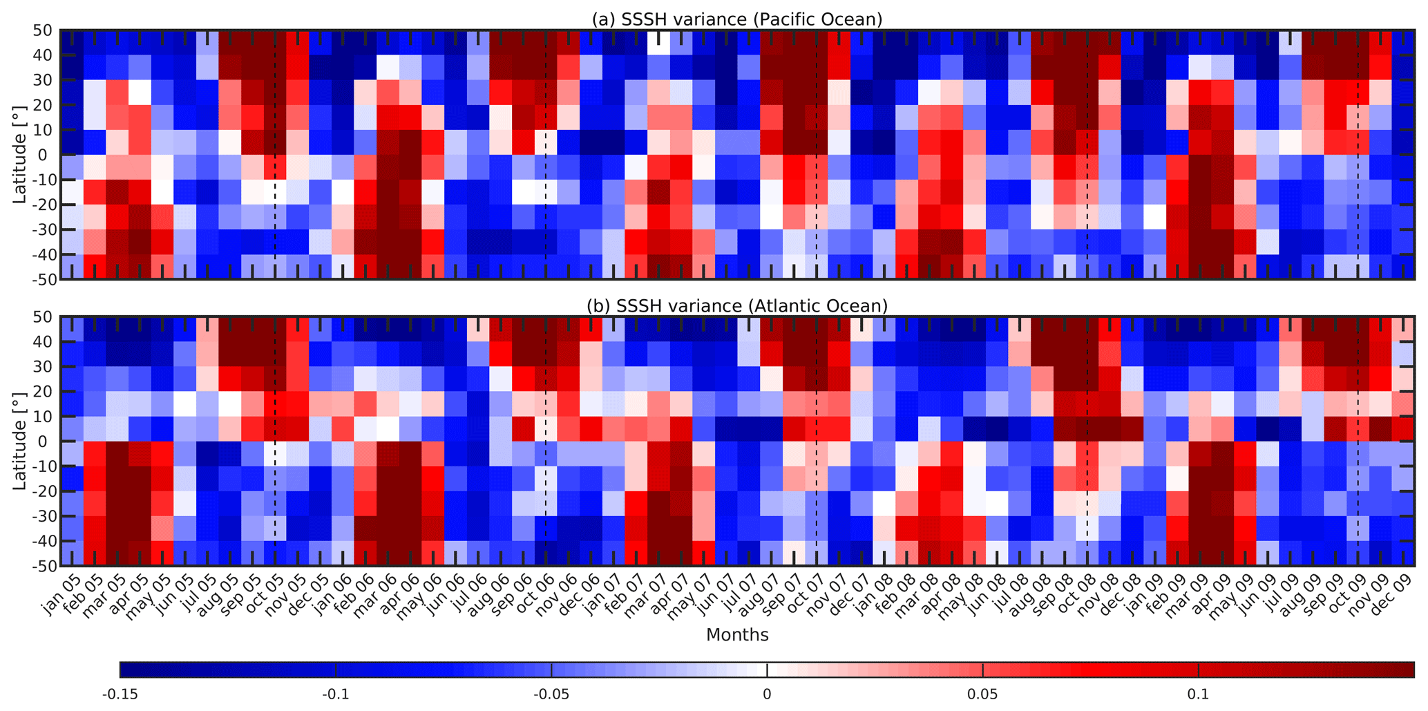
Figure A1 Zonally averaged anomaly time series of monthly variance in semidiurnal SSSH from expt 18.5 for the (a) Pacific and (b) Atlantic oceans. The anomalies are computed by removing and normalizing by the annual mean values.

Appendix B: Seasonal trends in non-normalized energy terms and steric sea surface height variance

Here, we show the seasonal trends for the non-normalized semidiurnal barotropic to baroclinic conversion rate, baroclinic energy flux, SSSH variance, baroclinic kinetic energy (KE), available potential energy (APE), and their sum for the Pacific and Atlantic oceans in Figs. B1 and B2, respectively. To compute the seasonal trends, we zonally average the conversion rate, flux, SSSH variance, KE, APE, and energy over 10° latitude bins for the Atlantic and the Pacific oceans for each 1-month segment. For all variables, shallow areas are removed (depth < 100 m). The anomalies are computed by removing the annual mean values. The non-normalized anomalies look similar to the normalized plots in Figs. 3 and 4, except at higher latitudes.

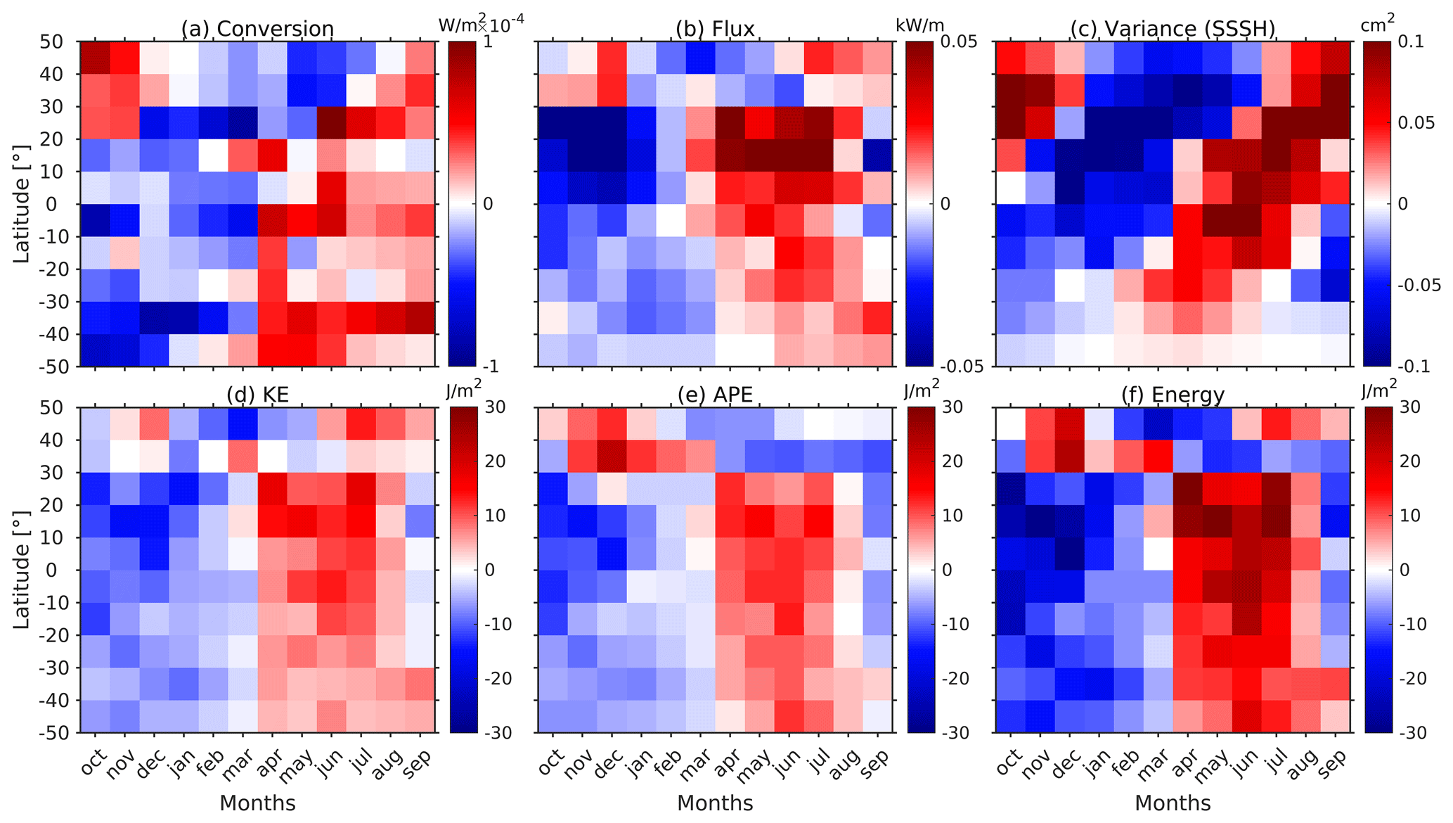
Figure B1 Zonally averaged anomaly time series of semidiurnal (a) barotropic to baroclinic conversion rate, (b) baroclinic energy flux, (c) SSSH variance, (d) KE, (e) APE, and (f) KE + APE for the Pacific Ocean. Data are from expt 06.1.

Figure B2 The same as Fig. B1, but for the Atlantic Ocean.

Appendix C: Georges Bank and the Arabian Sea

In Section 3.3, we showed that KE, conversion rate, and SSSH variance exhibit similar seasonal trends in Georges Bank and the Arabian Sea (Fig. 5i, j, o, and p). Furthermore, the seasonal variability is strongest in these two regions (Fig. 2a and c). In this section, we aim to understand the mechanisms causing the seasonal variability in the semidiurnal internal tides in these areas. Specifically, we investigate the impact of changes in the vertical profile of stratification on the barotropic to baroclinic conversion throughout the year. To do this, we calculate the vertical profile of the conversion rate using the following equation (Kang and Fringer, 2012):

$$\begin{array}{}\text{(C1)}& C_v\left(z\right)={\displaystyle \frac{\mathrm{1}}{T}}\underset{\mathrm{0}}{\overset{T}{\int }}{\mathit{\rho }}^{\prime }(z,t)gW(z,t)\mathrm{d}t,\end{array}$$

where $W\left(z\right)=-W(z=-H)\frac{z}{H}$.

Georges Bank and the Gulf of Maine are located in the Northwest Atlantic Ocean. Internal tides are generated on the northeast flank of Georges Bank and the Northeast Channel in this region (Fig. 1b) (Chen et al., 2011; Schindelegger et al., 2022). The M₂ barotropic tides are strong in this area, but there are only small seasonal changes in barotropic sea surface height amplitude (Godin, 1995; Katavouta et al., 2016). However, studies have reported seasonal changes in tides related to stratification in the Gulf of Maine (Chen et al., 2011; Katavouta et al., 2016; Shen et al., 2020; Schindelegger et al., 2022). To understand the mechanisms causing the seasonal variability, we compare the conversion rate and buoyancy frequency for the location where the conversion rate is at its maximum (42.09° N, 294.48° E). We compare the depth-integrated and monthly mean conversion rates calculated with Eq. (6) (method 1) and Eq. (C1) (method 2) and observe that both methods yield similar values (Fig. C1a). Additionally, we observe a similar seasonal cycle for the depth-integrated conversion rate and depth-averaged buoyancy frequency at this location. Interestingly, we discover that when stratification is stronger near the surface (depths less than 100 m), the conversion rate is also higher for those months throughout the entire water column (Fig. C1c and e). The factors affecting stratification in Georges Bank are summer surface heating, surface heat transfer and cold winds during winter, interaction between the Gulf Stream and the southward movement of Labrador Sea water, and advection due to eddies (McLellan, 1957; Gatien, 1976; Brown and Beardsley, 1978; Csanady and Hamilton, 1988; Petrie and Drinkwater, 1993; Katavouta et al., 2016).

In the Arabian Sea region, strong internal tides are generated on the shelf break, which generally propagate offshore (Zhao, 2019; Zaron, 2019; Subeesh et al., 2021; Ma et al., 2021). On the slope, internal tides are stronger in March than in July due to the deepening of the pycnocline during the pre-monsoon period (Subeesh et al., 2021). In the Arabian Sea, the monsoonal winds, which change direction seasonally (Clemens et al., 1991), influence ocean circulation (Shetye et al., 1990, 1991; Beal et al., 2013) and are responsible for changes in pycnocline depth (Rudnick et al., 1997). We compare the vertical profile of the barotropic to baroclinic conversion with buoyancy frequency in Fig. C1 for a location where the conversion rate is maximum (18.24° N, 430.64° E). We get similar results for the depth-integrated and monthly mean conversion rates calculated for the two methods as shown in Fig. C1b. In contrast to Georges Bank, the seasonal trends in depth-integrated conversion rate and depth-averaged buoyancy frequency are not similar. We observe that the conversion rate is large for the months where the magnitude of buoyancy frequency is high at the greater depths (150–250 m) (Fig. C1d and f).

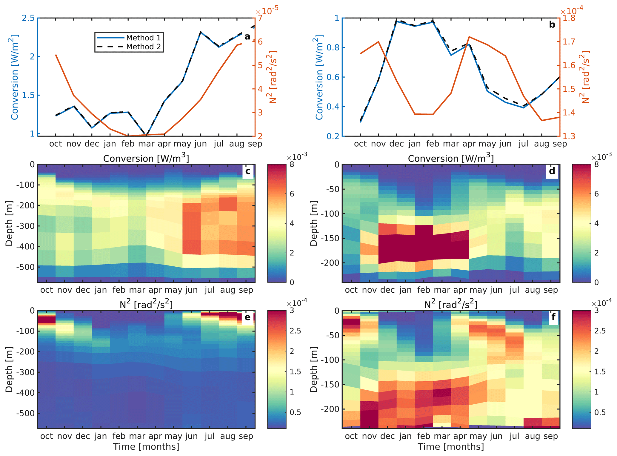
Figure C1 (a, b) Time series of monthly mean depth-integrated conversion and depth-averaged buoyancy frequency for a location on the shelf slope in Georges Bank (left column) and the Arabian Sea (right column). Methods 1 and 2 represent the depth-integrated conversion computed using Eqs. (6) and (C1), respectively. (c, d) Vertical conversion profile and (e, f) vertical buoyancy frequency profile for Georges Bank (left column) and the Arabian Sea (right column). Data are from expt 06.1.

In conclusion, at both Georges Bank and the Arabian Sea, the seasonality in stratification greatly affects the conversion. However, at Georges Bank, these stratification changes occur mainly at the surface, whereas in the Arabian Sea, these changes mostly take place at depth.