the Creative Commons Attribution 4.0 License.
the Creative Commons Attribution 4.0 License.
 | 12 Sep 2024
Exploring variability in climate change projections on the Nemunas River and Curonian Lagoon: coupled SWAT and SHYFEM modeling approach
Natalja Čerkasova
Rasa Idzelytė
Jūratė Lesutienė
Ali Ertürk
Georg Umgiesser
This study advances the understanding of climate projection variabilities in the Nemunas River, Curonian Lagoon, and southeastern Baltic Sea continuum by analyzing the output of a coupled ocean and drainage basin modeling system forced by a subset of climate models. A dataset from a downscaled high-resolution regional atmospheric climate model driven by four different global climate models was bias-corrected and used to set up the hydrological (Soil and Water Assessment Tool, SWAT) and hydrodynamic (Shallow water HYdrodynamic Finite Element Model, SHYFEM) modeling system. This study investigates the variability and trends in environmental parameters such as water fluxes, timing, nutrient load, water temperature, ice cover, and saltwater intrusions under Representative Concentration Pathway 4.5 and 8.5 scenarios. The analysis highlights the differences among model results underscoring the inherent uncertainties in projecting climatic impacts, hence highlighting the necessity of using multi-model ensembles to improve the accuracy of climate change impact assessments. Modeling results were used to evaluate the possible environmental impact due to climate change through the analysis of the cold-water fish species reproduction season. We analyze the duration of cold periods (<1.5 °C) as a thermal window for burbot (Lota lota L.) spawning, calculated assuming different climate forcing scenarios and models. The analysis indicated coherent shrinking of the cold period and presence of changepoints during historical and different periods in the future; however, not all trends reach statistical significance, and due to high variability within the projections, they are less reliable. This means there is a considerable amount of uncertainty in these projections, highlighting the difficulty of making reliable climate change impact assessments.
- Article
(8456 KB) - Full-text XML
- BibTeX
- EndNote


A river–lagoon–sea continuum is a very complex system that forms a unique and vulnerable environment, providing a broad spectrum of the ecosystem services (Kaziukonytė et al., 2021; Inácio et al., 2018) and playing an important socioeconomic role. On a larger scale, the climate change impacts are extensively analyzed and already shows that the coastal zone will be impacted by global warming and sea level rise by altering freshwater runoff, frequency and intensity of coastal storms, and precipitation and nutrients patterns (Viitasalo and Bonsdorff, 2022; Lu et al., 2018). Modeling becomes an important tool to project climate change impact, with the focus on the intensity and direction of future changes. However, there are a lot of uncertainties regarding the trends and projected impacts due to climate change (IPCC, 2013). The uncertainties and variations in projected future scenarios emerge due to unknowns in global or regional climate models (GCMs and RCMs), proposed scenarios (RCPs), or statistical techniques used for data preparation. Therefore, uncertainty analysis is commonly used to quantify the possible discrepancies between the projections and their impacts on possible future changes. There is a wide variety of studies focused on quantification of climate projection uncertainties around the world, including Lithuania (e.g., Chen et al., 2022; Song et al., 2020; Akstinas et al., 2019). Most of these studies analyze only hydrological changes due to meteorological input.
The uncertainty in climatic studies arises from various factors, as highlighted by Foley (2010). One key factor is the scenario used as the basis for climatic projections. These scenarios range from significantly reduced CO2 emissions to business-as-usual cases, i.e., continuation of high-emission-based economic growth, leading to vastly different climate trajectories (Latif, 2011; Taylor et al., 2012). Even if the underlying assumptions are consistent, the climate models used handle the physics differently, leading to different results of the key parameters (Lehner et al., 2020). Apart from the atmospheric models, there is also a variety of ocean models – for example, NEMO (Madec et al., 2016), POM (Mellor, 2004), ROMS (Shchepetkin and McWilliams, 2005), MITgcm (Marotzke et al., 1999), SHYFEM (Umgiesser et al., 2004), and others – which have to be considered. All of these models have different discretization, resolution, and representation of the physics modeled. Drainage basin models crucially depend on the changing land use of the basin (Wang et al., 2012; Lin et al., 2015; Waikhom et al., 2023), with subsequent effects on downstream coastal ecosystems.
The development of integrated modeling tools is a high-priority task that supports the management of the ecosystems at the land–sea interface, prone to both the riverine effects and the sea level rise. This study is a continuation of the previously published paper by Idzelytė et al. (2023a), where the framework of coupled hydrological and hydrodynamic models was used to explore future climate scenarios based on the ensemble mean values for the Nemunas River watershed, Curonian Lagoon, and Baltic Sea continuum. Here, we explore a subset of the possible variation space. We look at different scenarios computed by different climate models using only one ocean model (Umgiesser et al., 2004) and one drainage basin model (Čerkasova et al., 2018). This allows us to come up with a reasonable estimate of the variability in climate projections, its impact on the hydrology, and its application to the ecological evaluation of the studied Nemunas River basin, the Curonian Lagoon, and the southeastern Baltic Sea system as a whole.
It is expected that explicit analysis of the climate scenarios will help decision-makers in the development of climate change adaptation and mitigation strategies, adjustment of water quality management, and achievement of regional nutrient policy goals and measures. The level of uncertainty is crucial in the decision-making process; therefore, we aim to test model averaging (Idzelytė et al., 2023a) versus the ensemble method, where we combine the results of several models to form an ensemble projection. The diversity in projections among the ensemble components may reveal the level of variability and aid in combining agriculture nutrient runoff policies with climate mitigation policies that involve integrating strategies to address the two issues simultaneously.
Climate prediction uncertainty has important implications for the conservation efforts of endangered or vulnerable species as meteorological-hydrological factors play a primary role in shaping species habitat conditions, life cycle completion, spread, and survival. In addition to the variability in projections for the region, we specifically tackle the question of how considerably the imposed changes could be reflected in ecosystem function and habitat conditions for the species. As the response of climate forcing is most pronounced in water temperature, we selected the stenotherm species burbot (Lota lota L.). As a cold-water fish species, the burbot is particularly sensitive to changes in thermal habitat availability (Harrison et al., 2016) and suffered severe declines throughout its distribution range worldwide (Stapanian et al., 2010). Evaluating the impact of climate change on spawning habitats is essential for projecting the future status of the vulnerable burbot population in the Curonian Lagoon.
2.1 Study area
Our study site is a large transboundary basin–coastal lagoon–sea system: the Nemunas River basin, the Curonian Lagoon, and the southeastern Baltic Sea. The Curonian Lagoon is a shallow estuarine lagoon located in the territories of Lithuania and Russian Federation and connected to the southeastern Baltic Sea through the narrow Klaipėda Strait (Fig. 1). The lagoon covers an area of 1584 km2, with its widest section stretching up to 46 km in the southern part. Conversely, in the northernmost part (Klaipėda Strait), it narrows down to approximately 400 m in width. The drainage area of the Curonian Lagoon covers 100 458 km2, of which 48 % lies in Belarus, 46 % in Lithuania, and 6 % in the Kaliningrad region. Previous hydrodynamic modeling studies revealed that the lagoon consists of two different regions from the water exchange point of view, a transitional region at the northern part of the lagoon and a stagnant southern region which has a considerably higher water residence time. The predominant flow of water is from the south to the north, discharging approximately 23 km3 yr−1 into the Baltic Sea.
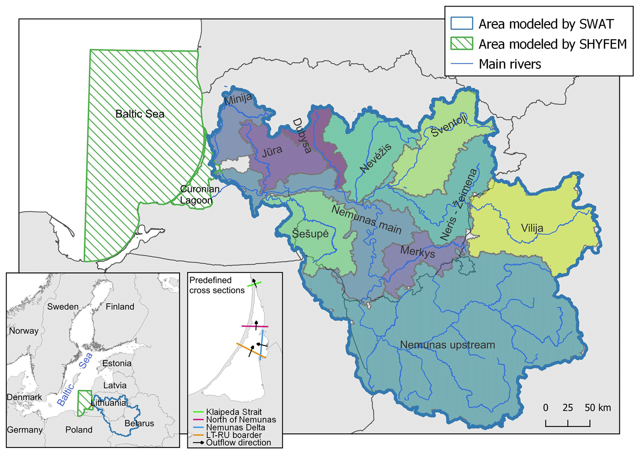
Figure 1Location of the Curonian Lagoon and Nemunas River watershed.
The largest river that discharges into the Curonian Lagoon is the Nemunas River, which, together with the Minija River, brings about 95 % of the total riverine input to the lagoon (Zemlys et al., 2013). Both rivers enter the lagoon in the middle of the eastern coast. The average annual discharge of the Nemunas River is 22–24 km3 (Umgiesser et al., 2016), and it exhibits a strong fluctuating seasonal pattern, peaking with snowmelt during the flood season in February–April. Due to discharge from the Nemunas River and other smaller rivers, the southern and central portions of the lagoon are considered to be freshwater.
The Curonian Lagoon and Nemunas Delta area both include protected territories with various statuses: biosphere polygons, reserves, Natura 2000 (special protection areas, EC Birds Directive; sites of community importance, EC Habitats Directive), and Ramsar List sites (List of Wetlands of International Importance) (Kaziukonyte et al., 2021). The Curonian Lagoon and Nemunas Delta are the most important areas for commercial fishing in Lithuania, contributing about 95 %–98 % of the total inland fishery (Ivanauskas et al., 2022). Bream (Abramis brama L.), pikeperch (Sander lucioperca L.), and smelt (Osmerus eperlanus L.) are the main commercial fish species in the lagoon. In the context of climate change, cold-water species like burbot (Lota lota L.) are particularly sensitive. They rely on low water temperatures during winter to initiate the spawning season.
2.2 Modeling system
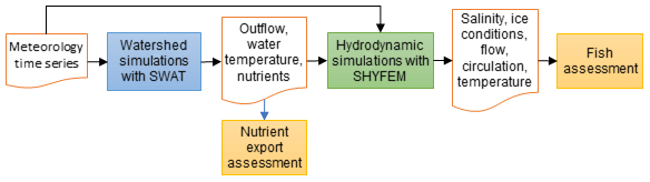
Due to limitations in current technology and tools, accurately representing the entire Nemunas River basin, Curonian Lagoon, and southeastern Baltic Sea system at high resolution with a single tool is impossible. As a result, we divided the area and utilized various modeling tools suited for specific purposes, which were then coupled. The modeling system that consists of two main models and numerous utilities mostly developed to transfer the outputs from one model as inputs to other models is summarized in Fig. 2. The system is characterized by two pivotal models: (1) the hydrological Soil and Water Assessment Tool (SWAT) model and (2) the hydrodynamic Shallow water HYdrodynamic Finite Element Model (SHYFEM). The SWAT and SHYFEM models depict main water flow dynamics in a Nemunas River watershed–Curonian Lagoon–Baltic Sea continuum.
The Nemunas River watershed is modeled using the SWAT model (Neitsch et al., 2009), which is widely used to simulate hydrological processes and water quality of watersheds. This model was developed, calibrated, and validated for the Nemunas River basin in previous studies (Čerkasova et al., 2021, 2019, 2018). SWAT is a comprehensive tool that requires numerous model inputs for hydrological parameterization and watershed characterization. The inputs can differ based on modeling demands and the topographic characteristics of the region. For the Lithuanian part of the watershed, regional high-resolution data (such as a digital elevation model, land use, soil, stream network, and reservoir information) were gathered from governmental institutions in Lithuania (see Table 1). Where data were not available, European or global datasets were used in combination with information found in relevant literature. To ensure accuracy, we manually digitized the stream network (used as the burn-in layer for watershed delineation and routing information), reservoir and pond geometry (used to identify the standing waterbody location and for parameter calculation), and major forest outlines (used to correct the land use layer).
Due to the large basin area and heterogeneity in topography and land management in the region, the entire watershed covering the entire Nemunas River basin was split into separate SWAT sub-models, each representing a sub-watershed of the main Nemunas River branch. Furthermore, to achieve better parametrization, a separate sub-model represents the Nemunas and all smaller tributaries situated in the territories of Belarus and Poland. The outcome of division into the sub-models produced the following configuration:
-
one sub-model in the Belarus territory (Neris in Lithuanian and
 in Belarusian);
 -
two transboundary watersheds, namely
-
Šešupė (
 in Russian and Szeszupa in Polish) and
 -
Nemunas upstream (
 in Russian and Belarusian);
-
-
seven sub-models with more than 95 % of the territory in the boundary of Lithuania or entirely situated in Lithuania, namely
-
Minija,
-
Merkys,
-
Jūra,
-
Dubysa,
-
Šventoji,
-
Nevėžis, and
-
Neris–Žeimena;
-
-
one sub-model, the main branch of Nemunas, discharging into the Curonian Lagoon.
A total of 11 sub-models were built, subdivided into subbasins (9012 in total), which were further subdivided into hydrological response units (HRUs; 148 212 in total), all of them configured, connected, and parametrized. The concept of the 11 SWAT models that are represented as sub-models for the entire study area is given in Fig. 1 (denoted as separate colors of the watershed). These models can be used individually or, as in this study, in a framework, where the upstream sub-models provide the input information to the downstream areas. Outputs from the main outlets on the Nemunas and Minija rivers were used as boundary conditions for the hydrodynamic model.
Calibration and validation of each sub-model were conducted manually by adjusting parameters linked to specific processes. The multisite calibration process followed an approach typical of hydrological models (Daggupati et al., 2015; Feyereisen et al., 2007). Calibration began with the upstream regions followed by the downstream areas, focusing on flow, sediment, total nitrogen (TN), and total phosphorus (TP). This methodology was applied to both individual sub-models and overall modeling framework. Details can be found in Čerkasova et al. (2021).
The hydrodynamics of the Curonian Lagoon and the southeastern Baltic Sea were simulated using the open-source Shallow water HYdrodynamic Finite Element model SHYFEM, accessible at https://github.com/SHYFEM-model/ (last access: 28 November 2023). The model uses an unstructured grid (finite elements) to discretize the studied basin (Curonian Lagoon and part of the Baltic Sea). The use of finite elements is crucial in order to simulate the narrow connection of the lagoon with the sea (Klaipėda Strait). However, it varies from 250 m close to the Klaipėda Strait to up to 2.5 km in the central part of the lagoon and up to 10 km in the Baltic Proper. The atmospheric forcing has been interpolated directly from the regular grid of the regional climate model data into the finite-element nodes by bi-linear interpolation. Lateral boundary conditions were taken from Copernicus data and interpolated onto the finite-element grid (water levels, T, and S). The COARE 3.0 module is used for bulk formulation. The model solves shallow water equations and, in this study, the two-dimensional version of the model was used. SHYFEM simulates key physical variables, such as circulation, waves, water level, temperature, and salinity fields, that are needed to characterize the water matrix. To compute the water fluxes across the sides of the elements, first, the conservation of mass in the finite volume around a node that is guaranteed by the continuity equation is used. The fluxes over the lines delimiting the finite volume element per element are made divergence-free by subtracting the storage of water inside the node. With these finite-volume fluxes, the fluxes over the element sides are computed. This tool has been applied to a large number of lagoons around Europe. Details can be found in Idzelytė et al. (2020), Umgiesser et al. (2004, 2014, 2016), and Zemlys et al. (2013).
2.3 Data
Our modeling system incorporates different input data, varying according to the specific model utilized – either hydrological or hydrodynamic (as outlined in Table 1). Given that this study follows the research conducted by Idzelytė et al. (2023a), to delve into the specifics of the input data utilized in our study, we refer the reader to their previously published work.
Table 1Input and validation data types for the hydrological and hydrodynamic modeling system and their respective sources.
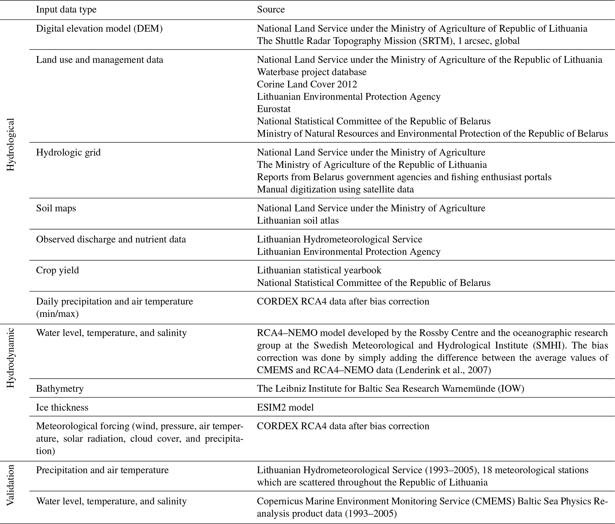
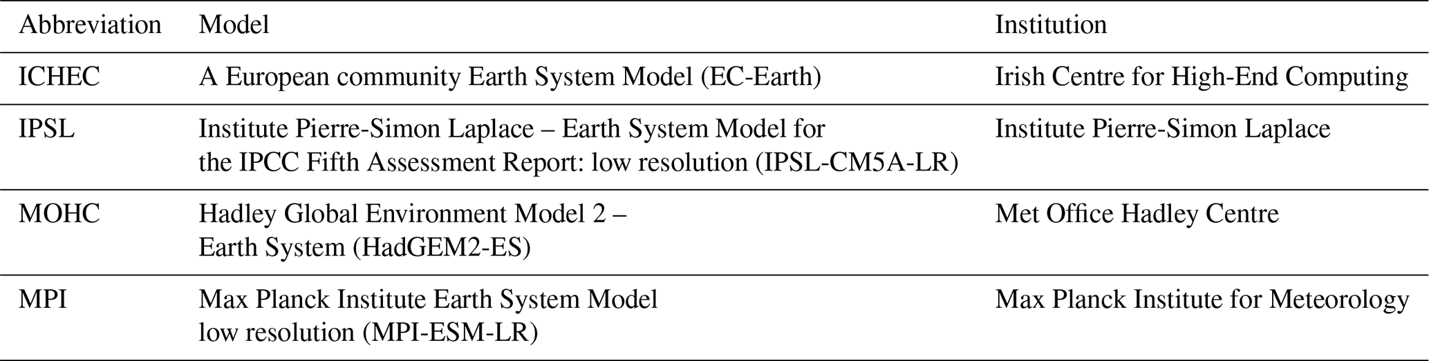
Both hydrological and hydrodynamic models were run using the same bias-corrected future meteorological forcing data described in Table 2. Data were obtained from CORDEX (Coordinated Regional Climate Downscaling Experiment) scenarios for Europe, employing the Rossby Centre high-resolution regional atmospheric climate model (RCA4). This involved four sets of simulations (downscaling), driven by four global climate models. The datasets are spanning the historical period of 1970–2005 and the projection period of 2006–2100. Projections are based on two Representative Concentration Pathway (RCP) scenarios, specifically RCP4.5 and RCP8.5 of the Coupled Model Intercomparison Project Phase 5 (CMIP5). The bias correction was conducted by applying the climate data bias-correction tool (Gupta et al., 2019). The ice thickness data utilized in our study were derived using ESIM2 (Enhanced Sea Ice Model) (Tedesco et al., 2009; Idzelytė and Umgiesser, 2021). This model was run independently, as a standalone system, and the resulting output time series were integrated into our hydrodynamic modeling framework as surface boundary input data. This approach allowed us to accurately incorporate ice thickness dynamics into our simulations, enhancing the overall reliability of our model during the ice season. A detailed description of all the datasets used for this study can be found in Idzelytė et al. (2023a), while the results derived from the modeling system can be found and accessed on the open-access Zenodo database (https://doi.org/10.5281/zenodo.7500744, Idzelytė et al., 2023b).
Table 2Meteorological forcing data sources for the hydrological and hydrodynamic modeling systems.
2.4 Analysis methods
2.4.1 Investigation of hydrological and hydrodynamic model results
The analysis was done for the environmental parameters corresponding to our preceding study (Idzelytė et al., 2023a). These include air temperature; precipitation; Nemunas River discharge; and water inflow and outflow from the lagoon at different locations, such as Klaipėda Strait, north of Nemunas, Nemunas Delta, and along the Lithuanian–Russian (LT–RU) border. In this analysis, we maintained the inflow and outflow categories as in our previous study (Idzelytė et al., 2023a). We analyzed the data by computing the 10-year moving average using yearly average fluxes, in this way ensuring an accurate representation of water flux dynamics throughout the study period. Water temperature and water level were evaluated for the southeast (SE) Baltic Sea and Curonian Lagoon. Saltwater intrusions (>2 g kg−1) were assessed in Juodkrantė, approximately 20 km south of Klaipėda Strait. Information on ice cover in the Curonian Lagoon encompasses the season duration and maximum thickness. Water residence time is analyzed for the northern and southern parts of the lagoon as well as the total lagoon area.
The analysis was done by combining historical (1975–2005) and future scenario projection (2006–2100) periods. That is, two periods/scenarios were assessed: RCP4.5 and RCP8.5, both ranging from 1975 to 2100. This approach facilitated a comprehensive assessment of the abovementioned environmental parameters, enhancing insight into trends and potential variations over time.
In our analysis, we examined the variability in different model runs and the presence of trends and their statistical significance, as indicated by the p values, across various environmental parameters under different climate models and scenarios. For this, we applied the Mann–Kendall trend analysis (Hussain and Mahmud, 2019). A p value less than 0.05 was considered statistically significant. The rate of change was quantified using the Theil–Sen estimator (Hussain and Mahmud, 2019). The trend analysis was conducted on model outputs, which were aggregated as yearly means or, in the case of precipitation, as a yearly sum.
The timing of spring peak flows was estimated by computing a 3 d moving average of the discharge of the Nemunas River to the delta region. The day of the maximum value during the typical spring flood window occurrence (from the start of February to the end of April) was noted for each year. The trend was calculated using the same Mann–Kendall trend analysis approach as described above, using the Julian day of peak flow for each year in the simulation period.
We analyzed the average annual export of total nitrogen (TN) and total phosphorus (TP) from the Nemunas River into the Curonian Lagoon. We assessed the trends using the Mann–Kendall test and the 10-year moving averages. These outputs were compared to the nutrient ceiling for the Nemunas River requirements outlined in the Helsinki Commission (HELCOM) Baltic Sea Action Plan (HELCOM, 2021), which is 29 338 t yr−1 for TN and 914 t yr−1 for TP. We further evaluated the feasibility of meeting these targets under the conditions of different scenarios and climate models.
The variability between the models, i.e., uncertainty, was assessed by computing the standard deviation and coefficient of variation using annual values over the entire investigation period (1975–2100). These metrics were based on the yearly average values of modeled parameters (or sum in the case of precipitation, ice season duration, and saltwater intrusions) for each of the four simulation results using meteorological forcing data from different climate models.
2.4.2 The possible impact on fish recruitment success
To evaluate the extent and possible impact of climate change on fish recruitment success, the analysis of the burbot spawning period was carried out. Burbot requires very cold temperatures (<2 °C) for spawning and egg development (Harrison et al., 2016; Ashton et al., 2019). Within the Curonian Lagoon, it moves to spawning habitats in the Nemunas River delta. Spawning is most intense at the lowest water temperatures (close to 0 °C) during December–February, usually under ice. The duration of the cold period in the projected time series of temperatures suitable for burbot spawning was calculated by summing days when temperature was below 1.5 °C for a given year (days in December were added to the next year). The R package changepoint (Killick and Eckley, 2014; Killick et al., 2022) was used to estimate the number and locations of changepoints in a time series of cold period duration. The changes in mean and variance at a single point were estimated using the cpt.meanvar function, employing the AMOC (“at most one change” method). The semi-automatic Pruned Exact Linear Time (PELT) algorithm was employed for the estimation of multiple changepoint locations and parameter estimates within segments (time periods). The number of changepoints was set to five using the parameter Q.
3.1 Ensemble dynamics
3.1.1 Water flows
There is a noticeable variability among the climate models in terms of the projected mean yearly water fluxes through the predefined lagoon's cross sections (Fig. 3). Despite this variability, a consistent pattern emerges across all models, with water outflow from the lagoon towards the sea being a prominent feature in every cross section examined. Each model captures unique hydrodynamic behaviors at different cross sections of the lagoon. Still, they all indicate that the cross sections of north of Nemunas and Klaipėda Strait generally experience higher water fluxes.
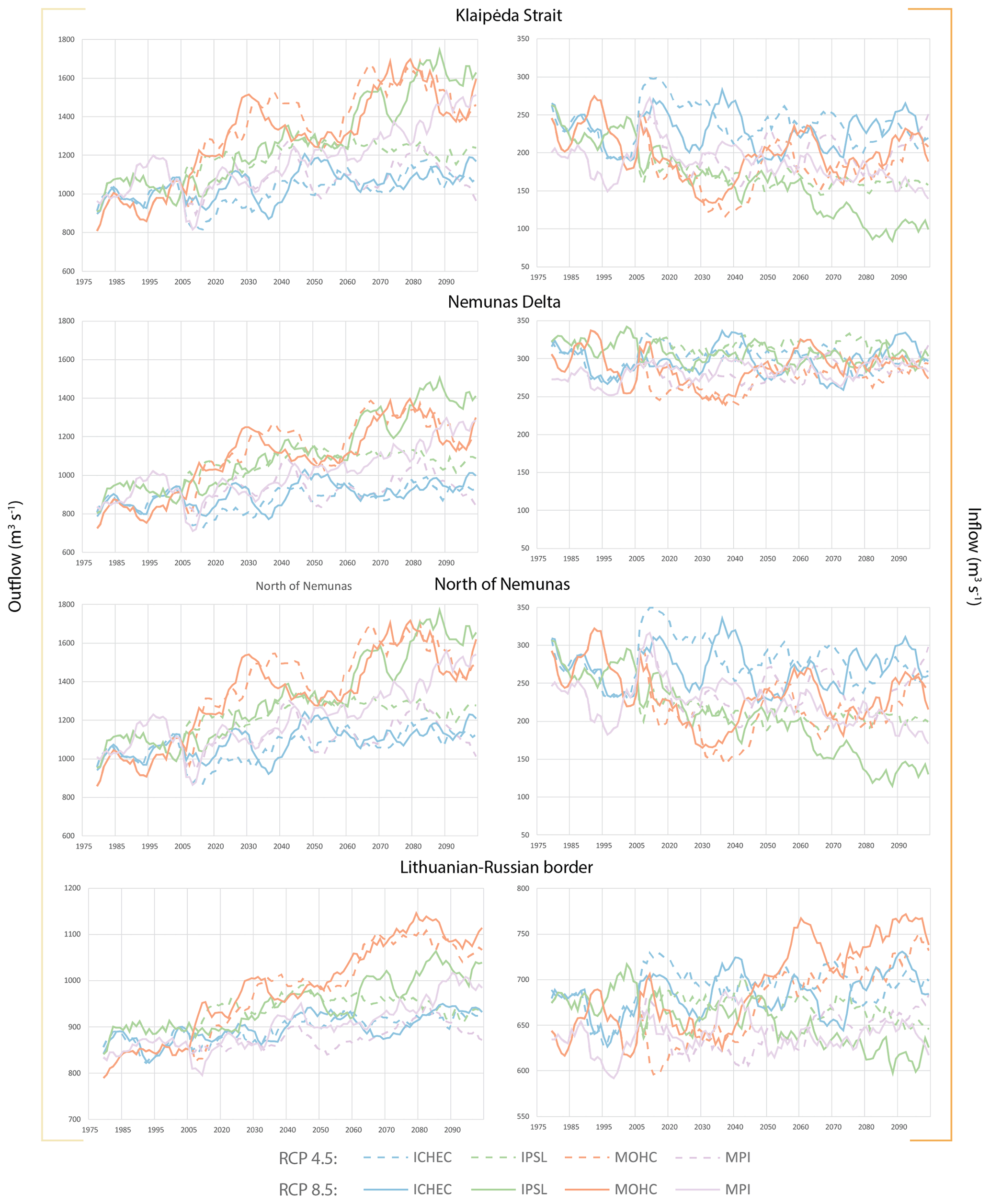
Figure 3Graphs showing the 10-year moving average of outflowing (left column) and inflowing (right column) water fluxes (in m3 s−1) across four cross sections within the Curonian Lagoon. Note the adjusted ranges of the y axis for fluxes passing through the Lithuanian–Russian border.
Across all models, the RCP8.5 scenario consistently results in higher mean outflowing water fluxes compared to RCP4.5, and the MOHC results stand out for consistently projecting the highest mean fluxes in both scenarios, suggesting a more pronounced increase in water movement through the lagoon compared to its counterparts. Both scenarios show a higher outflow to the sea discharge, with a possible increase of to m3 s−1 by the end of the century. These results could lead to the outflow from the lagoon reaching 37.8–50.4 km3 yr−1, which is 24 %–165 % higher compared to historical outflow.
Regarding the inflowing water fluxes from the Baltic Sea into the Curonian Lagoon, the IPSL model generally predicts lower fluxes in both scenarios compared to the other models. Inflowing fluxes through the Lithuanian–Russian border show the least variability in predictions across models, especially under the RCP8.5 scenario, indicating a consensus on the water flux through this cross section.
Regarding water residence time (Fig. 4 and Figs. A1 and A2 in Appendix A), IPSL tends to predict the shortest water residence times, suggesting a model inclination towards faster water turnover in the lagoon. In contrast, ICHEC and MPI, with their higher values, may incorporate factors leading to longer residence times. The shift from RCP4.5 to RCP8.5 and between different analysis areas does not uniformly affect the models.
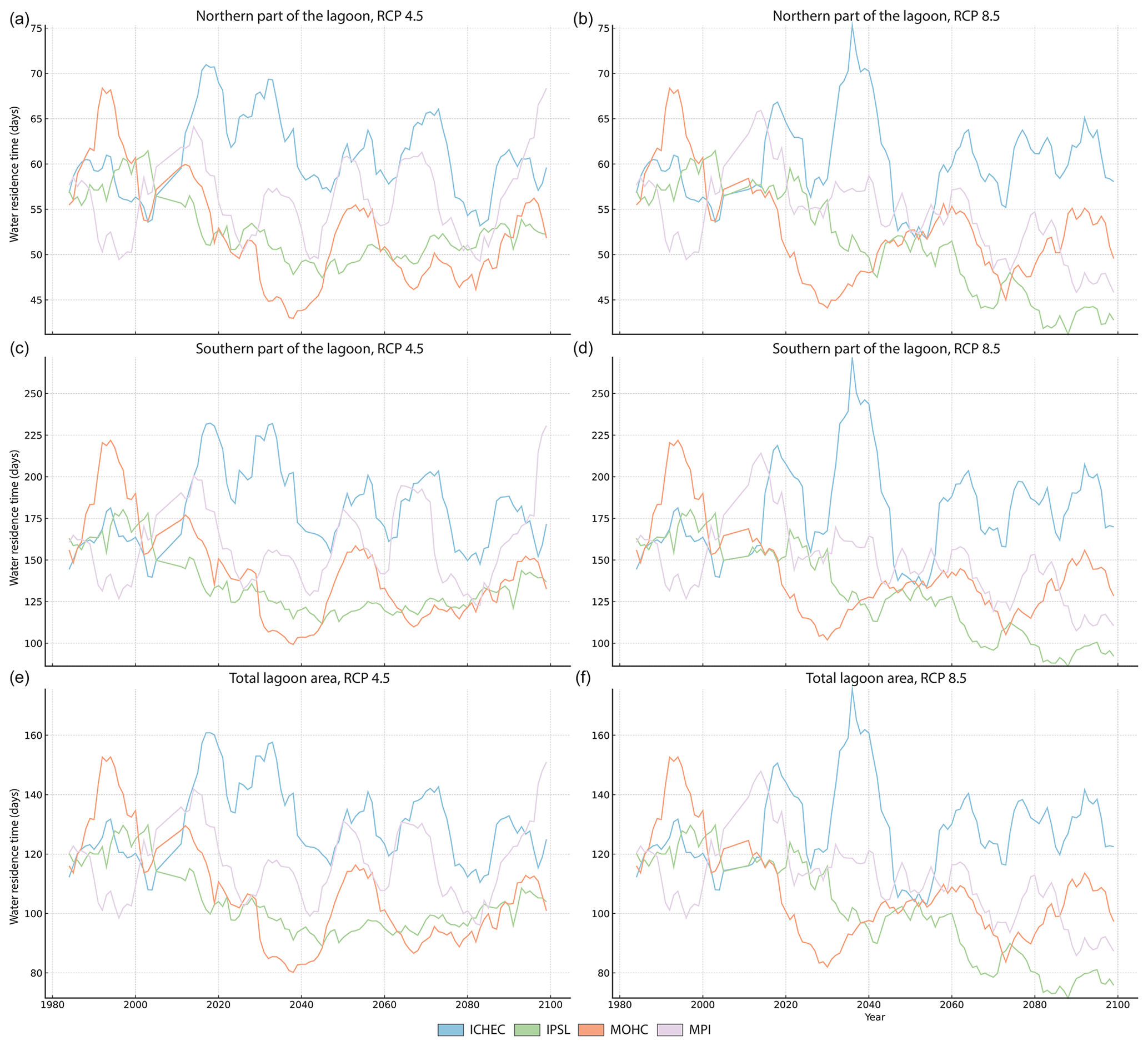
Figure 4The timing of the annual water residence times (in days) in the north (a, b) and south (c, d) parts of the lagoon and the total lagoon area (e, f) for both RCPs.
3.1.2 Timing of peak flows
The high discharge of the Nemunas River and subsequent flooding of the delta region is a nearly annual event which occurs in the late winter–spring season and is referred to as the “spring flood” in Lithuania. We use the same term in this study and consider the historic period of high river flows to be from 1 February to 30 April. The timing of spring floods in the Nemunas River delta was previously reported to shift to earlier days due to climate change (Čerkasova et al., 2021). Further statistical analysis of the projected flows shows that overall there is a statistically significant relationship between the independent variable “year” and the Julian day of occurrence of peak flows in the Nemunas River for both RCPs when analyzing the entire period (Fig. 5).
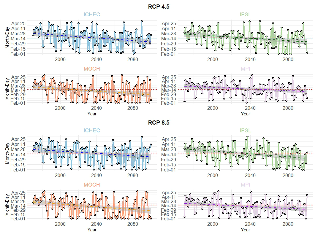
Figure 5The timing of occurrence of the average 3 d maximum flow rate in the spring (between 1 February and 30 April) of the Nemunas River to the delta region, with a trend line for each model. The horizontal red line depicts the period's middle date of 15 March.
The graphs show that the projected timing of spring high flows is expected to advance in all climate change scenarios, meaning that the maximum flows are expected to occur earlier in the year. The magnitude of the advance is greater for the higher-emission scenario (RCP8.5). Both IPSL and MOHC project a higher magnitude of change, judging by the steepness of the slope, whereas ICHEC and MPI project a moderate rate of change. This could have several impacts, such as disrupting fish spawning cycles and increasing the risk of flooding.
3.1.3 Nutrient loads
The projections suggest varying levels of variability and trends in the TN and TP loads from the Nemunas River across different RCPs and models (Fig. 6). RCP8.5 generally projects higher TN and TP loads compared to RCP4.5 for all models. This suggests that more extreme climate change scenarios lead to higher nutrient loads in the study region.
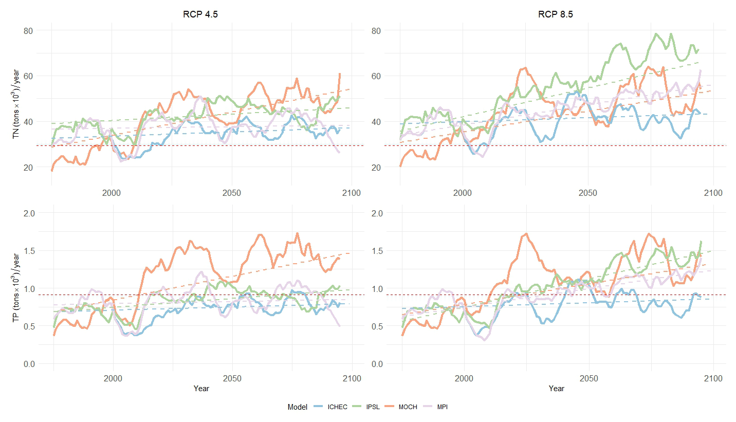
Figure 6The projected 10-year moving average of the annual mean TN and TP loads from the Nemunas River to the lagoon, with a trend line for each model. The horizontal red line depicts the revised nutrient input ceiling for the Nemunas river defined by the BSAP update (HELCOM, 2021).
The projected TN loads are expected to remain above the revised nutrient input ceiling for all four climate models and both climate change scenarios (RCP4.5 and RCP8.5) throughout the entire simulation period (shown as a red line in Fig. 6). Overall, the graph suggests that even in the stabilization scenario (RCP4.5), TN loads from the Nemunas River are expected to remain above the BSAP (Baltic Sea Action Plan) targets. Total P loads can fall below the maximum target during several brief periods, but the timing of this will depend on the actual climate scenario that unfolds. There is substantial variability between the models, which indicates a high level of uncertainty in the projections. Notably, under the condition of the MOHC model, the TP projections elevate mid-century and further stabilize at high loads by the end of the modeled period. The IPSL for RCP8.5 projects higher loads, whereas ICHEC and MPI display a moderate increase (Fig. 6). The lowest average annual nutrient load is projected under the ICHEC conditions for both RCPs.
3.1.4 Saltwater intrusions
The data of the number of days of saltwater intrusion events, i.e., when salinity in Juodkrantė exceeds the 2 g kg−1 threshold, show yearly variations across different models (Fig. 7). All models exhibit considerable year-to-year variability in the number of saltwater intrusion days, highlighting the complex interplay of climate variability and local hydrological processes affecting the intrusions. Both ICHEC and MPI often show higher numbers of saltwater intrusion days compared to IPSL and MOHC. When comparing the RCP4.5 scenario with RCP8.5, the models yield varying results; ICHEC and IPSL show a slight decrease in intrusion days, MOHC slightly increases, and MPI shows a moderate decrease.
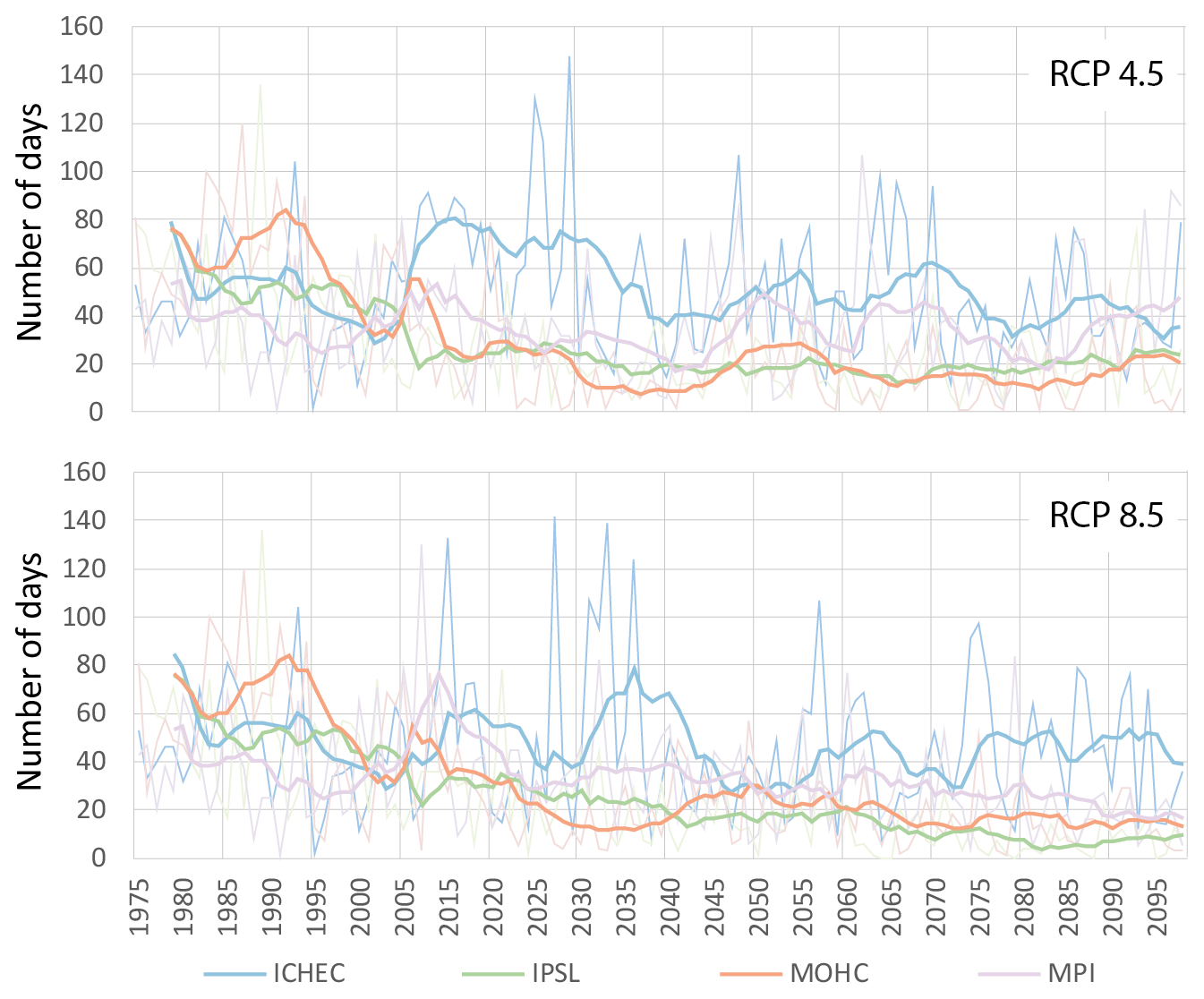
Figure 7Graphs showing the 10-year moving average of the number of days of saltwater intrusions (salinity exceeding 2 g kg−1 threshold) reaching Juodkrantė. Underlying time series denote annual saltwater intrusions.
3.1.5 Water temperature
The annual mean water temperature within the lagoon and adjacent coastal areas is depicted in Fig. 8. Under the severe RCP8.5 scenario, hydrodynamic model simulations predict a noticeable increase in both mean water temperatures and their variability compared to the RCP4.5 scenario, indicating higher temperatures with greater uncertainty ahead. The IPSL model consistently projects slightly warmer temperatures across scenarios, while the MOHC model shows the largest jump in variability, suggesting that it predicts greater uncertainty for RCP8.5. Despite model variations, the trend towards warmer and more uncertain climate conditions is universally acknowledged.
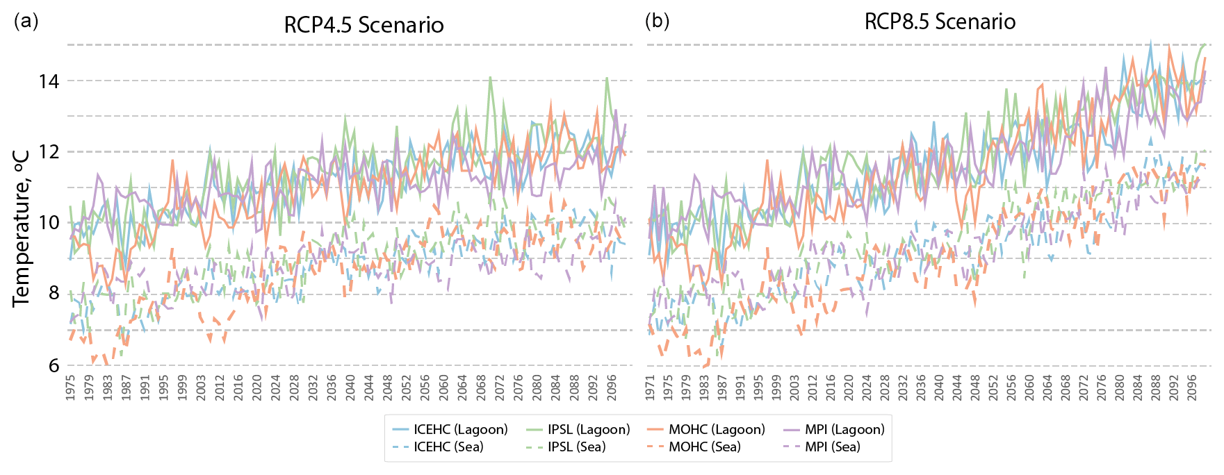
Figure 8Graphs showing the 10-year moving average of annual mean water temperature in the Curonian Lagoon and southeastern coastal area of the Baltic Sea.
3.1.6 Ice thickness
The comparative analysis of climate model projections for maximum ice thickness and ice season duration (Fig. 9) highlights the diverse outcomes projected by different model simulations over time and through various scenarios. All models indicate a shortening of the ice season and thinning of the ice. Notably, the MOHC model often showed lower thicknesses and shorter ice season duration compared to other models with a distinctive sinusoidal pattern. In contrast, ICHEC indicates a more gradual decline in ice season duration, whereas IPSL and MPI exhibit a greater variability over the years. Regarding maximum ice thickness, ICHEC and MPI show higher year-to-year variability.
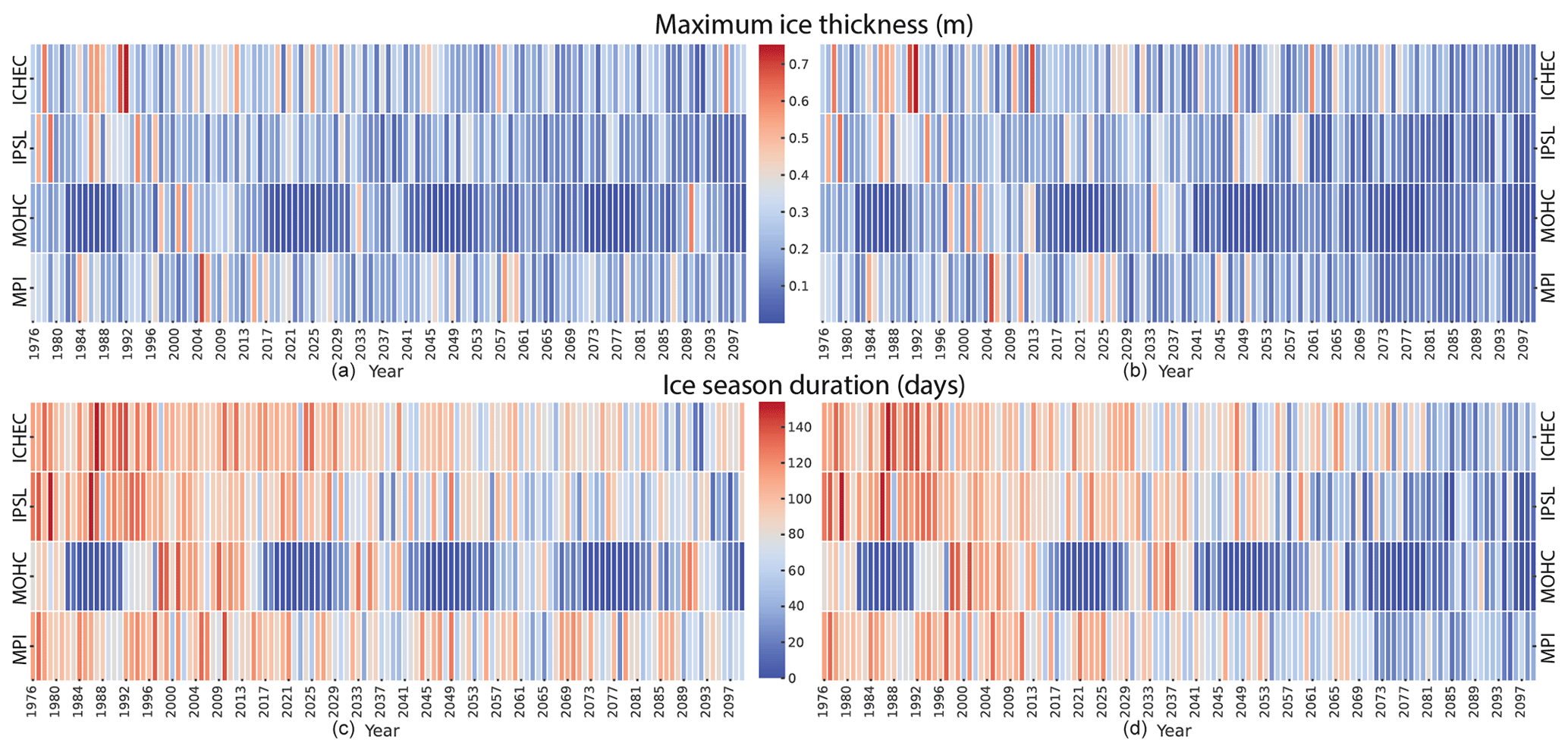
Figure 9Heatmaps of maximum ice thickness and ice season duration in the Curonian Lagoon for RCP4.5 (a, c) and RCP8.5 (b, d).
3.2 Trend analysis
Table 3 provides a comprehensive overview of trends, accompanied by their statistical significance (p values) and the rate of change (Theil–Sen estimator) for various environmental parameters in different climate scenarios. The results revealed that numerous parameters exhibited significant trends over time. Notably, air temperature and precipitation consistently show significant increasing trends in all scenarios. Although the rate of change varies among the climate models, precipitation exhibits a more pronounced increase compared to air temperature. Water temperature and water level also consistently exhibit increasing trends in all scenarios.
Table 3Mann–Kendall trend analysis results. Trends and their significance (p values assessed at a 0.05 confidence level) with their rate of change (Theil–Sen estimator) of key environmental parameters throughout historical and RCP4.5 and 8.5 scenarios in different geographical locations within the Curonian Lagoon and southeastern (SE) Baltic Sea. Cells are colored based on the direction of the trend.
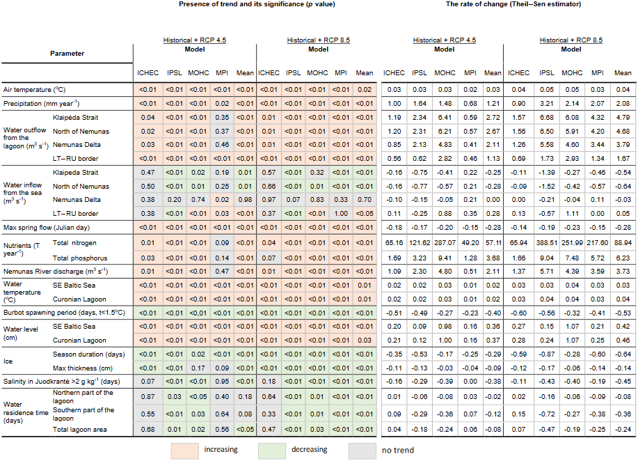
The MPI model exhibited the most frequent instances of statistically insignificant trends across the projected parameters. Notably, water inflow/outflow, nutrient discharge, riverine discharge, ice thickness, salinity, and water residence times all failed to meet the p<0.05 significance threshold. Interestingly, the MPI model produced the highest p value (0.02) for precipitation, which is the primary driver of other hydrological and hydrodynamic conditions in the model. It is worth noting that if the threshold for statistical significance were to be further reduced (e.g., p<0.01), the results for the MPI model could be entirely dismissed. This highlights the importance of carefully considering the chosen significance level when interpreting model outputs.
Theil–Sen slope estimates reveal a consistent pattern of increasing river discharge, nutrient loads, and water outflow across all projections. Conversely, consistent with these rising outflows, negative slopes were observed for inflows from the sea and salinity. These findings collectively suggest a projected increase in freshwater input to the Curonian Lagoon, potentially impacting its biological communities.
Figure 10 highlights a critical limitation of analyzing ensemble means alone: it can obscure the heterogeneity present within individual model projections. This is evident in the water inflow at the LT–RU border, where two models show statistically insignificant trends, yet the ensemble mean indicates a significant trend. Similarly, the individual model slopes for IPSL (−0.25) and ICHEC (0.88) portray contrasting projections (decrease vs. increase) compared to the ensemble mean (0.28), which leans towards an increase. These observations emphasize the importance of considering the spread of individual model projections and their uncertainties rather than solely relying on the ensemble mean.
3.3 Variability in the projections
Analysis of standard deviation (SD) values offers a comprehensive insight into the variations across simulation results using forcing from different climate models, while coefficients of variation (CV) provide a standardized measure of relative variability across the assessed environmental parameters (Table 4). Air and water temperatures have relatively low SD values. However, the deviation is more pronounced under the RCP8.5 scenario. Additionally, the SD is higher for air temperature compared to water temperature. In the case of precipitation, the SD presents more diverse results between the models, adding to the uncertainty in the modeling results.
Table 4Standard deviations of key environmental parameters throughout historical and RCP4.5 and 8.5 scenarios in different geographical locations within the Curonian Lagoon and southeastern (SE) Baltic Sea. Cells are colored based on the coefficient of variation.
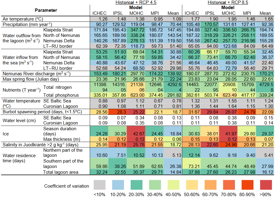
The low p values (Table 3) indicate that the trends in earlier maximum spring flows are statistically significant. Variability in the SD values across models and RCPs (Table 4) suggests that there is uncertainty associated with these projections. The range of Theil–Sen slopes also indicates variability in the rate of decline in the timing of maximum spring flows across different scenarios. Therefore, while the trends are significant, the variability in the projections should be considered when interpreting and using these results for decision-making. The SD values for the occurrence of maximum spring flows range from 21.79 (in the MPI 4.5 scenario) to 28.05 d (in the MOHC 8.5 scenario), where higher SD values indicate greater variability in the predicted time series data. Both IPSL and MPI models have lower prediction variability, whereas MOHC and ICHEC display larger variability. The RCP8.5 scenario indicates a greater degree of change, which is consistent with previous studies (Idzelytė et al., 2023a; Čerkasova et al., 2021). For both RCP4.5 and RCP8.5, the MPI model has the lowest CV (29 % and 32 %), while the MOHC model has the highest CV (38 % and 40 %). Based on these results, it can be concluded that the MPI model appears to be less variable compared to the other models for both RCP4.5 and RCP8.5 scenarios. Conversely, the MOHC model appears to be more variable compared to the other models for both scenarios.
The analysis of potential future TN and TP loads in the Nemunas River reveals a broad spectrum of possibilities. The variation is linked to the specific climate model and RCP scenario chosen. However, a consistent trend emerges across all models and RCPs – an upward trajectory for nutrient loads. Anthropogenic activities are the primary driver of nutrient loading from land sources. While climate factors, such as increased precipitation and subsequent nutrient wash-off, might exert a net negative impact on loads, a comprehensive future outlook requires incorporating anticipated changes in nutrient management practices and land use. This study acknowledges the omission of these factors, highlighting the need for further analysis to identify the most probable scenario and develop potential mitigation strategies for nutrient pollution in the Nemunas River.
When examining water dynamics within the lagoon, areas with greater fluctuations in SD are notably found in regions where water flow is more intense. This pattern is particularly different from the Nemunas Delta going northward to the Klaipėda Strait. Variability is much higher for water outflow than inflow. The most significant variation between the models is evident under the RCP4.5 scenario, where simulation results derived using MOHC datasets produce much higher SD than other models. A similar pattern is also evident for the ice season duration, while SD for saltwater intrusions in the lagoon is relatively similar between the different models. Water residence time exhibits the same variability between the models in all analysis sections. Notably, the IPSL model demonstrates a lower SD under the RCP4.5 scenario, while the ICHEC model exhibits a higher SD under the RCP8.5 scenario.
In almost all instances except for water level, the SD statistics derived from the model-averaged datasets exhibit lower values. This suggests a reduction in variability compared to individual models, emphasizing the smoothing effect achieved through model averaging. The most pronounced disparity in SD among the models is observed in the case of MOHC, particularly regarding the RCP4.5 scenario.
The differences between climate models become more apparent when considering coefficients of variation. While air and water temperatures show results that are relatively consistent with low CV values, parameters like salinity and ice-related variables display higher CV values, highlighting greater variability and uncertainty among the climate models. Among the parameters indicating water flow dynamics in different areas of the Curonian Lagoon, a clear disparity of the MOHC model can again be seen. This indicates the model's distinct response and emphasizes the need for careful consideration when employing the data of this climate model in hydrodynamic and hydrological simulations.
3.4 Changepoint analysis of burbot spawning period time series
The single-changepoint analyses of major shifts in mean and variance in time series of the duration of the cold season suitable for burbot spawning occur from 2013 to 2029 according to modeling results of RCP4.5 (Fig. B1 in Appendix B). The mean value of the time segment involving historical and recent past varies from 47 (MOHC RCP4.5) to 72 d (ICHEC RCP4.5). In the next period, it becomes shorter by 66 % according to MOHC and IPSL models and by 36 % and 51 % according to MPI and ICHEC models, respectively, taking no longer than 1 month. In three of the four RCP8.5 scenario models, the single changepoint could only be detected at the end of the time series, after 2040–2060, when the cold period duration is reduced to 6 to 9 d. An exception was generated by ICHEC RCP8.5 model results, indicating a changepoint in the historical past and showing that the duration of the cold period already decreased by 60 % in 1992 (Fig. B1 in Appendix B). Somewhat surprisingly, no changepoints in terms of variance are detected in the IPSL and ICHEC time series. Change in variance was detected in the IPSL time series in 1995 and in the MOHC time series in 2003 and 2013 (Fig. B2 in Appendix B), so both occurred within the historical period. Both model results indicate a variance of the cold period duration that is 2 to 3 times higher in the historical period than in the post-changepoint period (Fig. B2 in Appendix B).
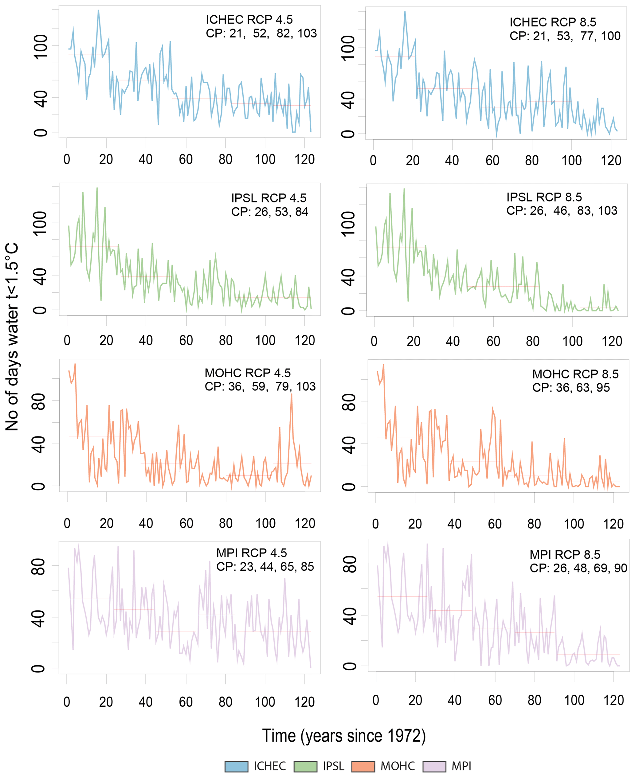
Figure 10Changepoint (CP) detection in the modeled time series of the burbot spawning period for the duration of t<1.5 °C conditions (Vente area). CP refers to changepoints indicated in a number of years since 1972.
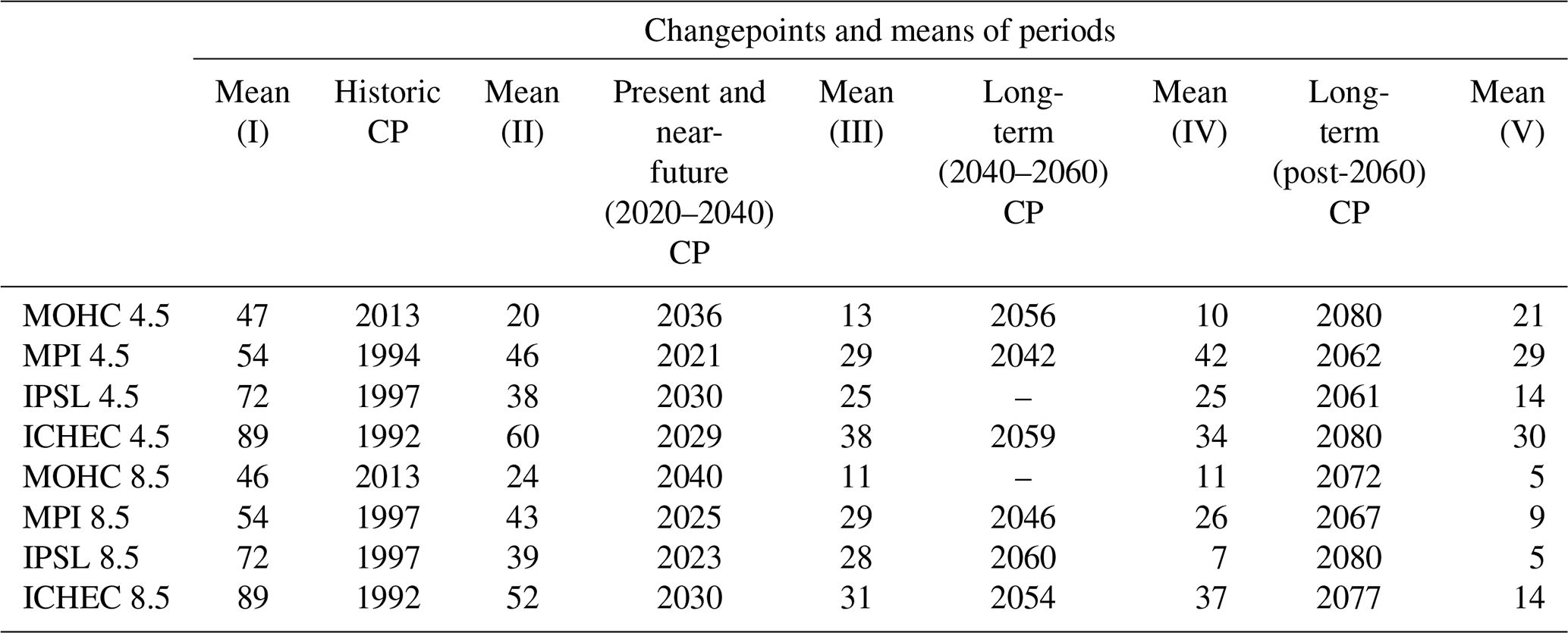
Multiple changepoint detection analyses indicated three to four changepoints in the modeled time series of cold period duration (Fig. 10). The significant decrease in a mean number of <1.5 °C days occurred in the 1990s according to MPI, IPSL, and ICHEC models, and the change was particularly obvious in the results of IPSL and ICHEC models at 46 %–47 % and 33 %–42 % reduction, respectively (Table 5). The cold period duration decreased from 3 to 2 months according to the ICHEC RCP4.5 model and to even less than 2 months in ICHEC RCP8.5 in 1992. The next time segment where all modeled time series had a changepoint is close to the present time and near future (Table 5). After this changepoint, the cold period further shrinks. If in the 1990s the MPI model showed only a slight decrease in the number of cold days (15 %), after 2021 (MPI RCP4.5) and 2025 (MPI RCP8.5), the reduction is more severe (46 %). After the second changepoint, 46 % to 72 % of the initial cold period duration is lost according to all model results. According to three out of four model results, the cold period duration is less than 1 month after the 2030s.
Table 5Multiple changepoints (CP; years) in modeled time series and mean values of the duration of the burbot spawning period (number of days when the temperature was <1.5 °C) in subsequent periods (I–V) at the Vente area.
Variability and uncertainty are not a flaw but a representative aspect of predicting complex systems. Multi-model ensembles (MMEs) are a vital tool in managing this uncertainty, providing a more robust and reliable basis for understanding future climate conditions and informing global efforts to mitigate and adapt to climate change. One common method to analyze MMEs for climate change impact assessment is ensemble averaging, which is often considered more accurate than any individual model's prediction, smoothing out model-specific biases. We performed this type of research in our previous study (Idzelytė et al., 2023a); however, investigating the dynamics of each model separately is important for evaluating the overall variability in impact predictions since relying only on multi-model averaging can obscure the detailed representation of extreme values and the variability in the parameters under study, potentially affecting the accuracy of projections (Tegegne et al., 2020).
In our study, two RCP model scenarios of one RCM driven by four GCMs were analyzed and each model showed independent variability in the parameters and its trends. In general, the trends are aligned in the same trajectory, but the slope differs: sharper decreases or increases occur in data series based on RCP8.5 forcing. Our study also indicates that even in the climate mitigation scenario RCP4.5, the changes in hydrological processes and temperature regimes are significant. The combined analysis of standard deviations and coefficients of variation provides valuable insights into the divergences between climate models in simulating hydrodynamic and hydrological processes.
4.1 Riverine inputs and water flows
The discharge of the Nemunas River exhibits a pronounced and statistically significant increasing trend accompanied by escalating rates of change. The overall water outflow from the lagoon also reveals increasing trends, suggesting changes in hydrological patterns, while water inflow varies in significance across scenarios and locations. The significance of the latter is inconsistent and varies between different climate models, with some of them (depending on the cross sections) displaying no significant trends, and others indicating a decrease in water inflow.
Results from the 10-year moving average imply much higher variability between the models in the long-term period, which reveals the cumulative effect of the uncertainties and complexity of the system. Our study results differ greatly compared to Jakimavičius et al. (2018) study based on the IPCC (2013) climate models without downscaling (GFDL-CM3, HadGEM2-ES, and NorESM1-M). The Jakimavičius et al. (2018) study applied the HBV (Hydrologiska Byråns Vattenbalansavdelning) hydrological model and used statistical methods to calculate the Baltic Sea parameters. With these techniques, the following main projected outputs were generated: (1) the Nemunas outflow decreases from 22.1 to 15.9 km3 with the RCP8.5 scenario, (2) the decreasing trend of the outflow to the sea induces only 0.7 % of the reference value, and (3) significant inflow increase to the lagoon due to sea level rise was calculated to be up to 61.3 % higher compared to the reference period (Jakimavičius et al., 2018).
Our study results are in line with Plunge et al. (2022), where the SWAT model with seven regional climate models was applied to test RCP4.5 and RCP8.5 scenarios. The Plunge et al. (2022) study projected the increase in the Nemunas River discharge by 9.7 % for RCP4.5 and by 35.4 % for the RCP8.5 scenario by the end of the century. The divergent results from various studies show the necessity to evaluate climate change scenarios with care. The use of the regional-bias-corrected data has a minor variation in the near future; however, the long-term projections are still uncertain. The trend analysis showed that the MOHC model projected the highest riverine input; as a result, most of the other parameters had more distinct results compared to those in other models.
The associated trends in water residence time (WRT) in different parts of the lagoon are diverse, with varying levels of significance and rates of changes. However, most of the RCP4.5 models did not show significant trends except for the mean trend for this scenario, while with RCP8.5 models, prevailing trends of decreasing water residence time can be observed. The decreasing trends can be explained by the higher Nemunas discharges and the increased outflow from the lagoon to the sea. Moreover, the timing of the maximum spring flood shifting to earlier days in the year could have important implications for the lagoon flushing rate in spring; for example, the absence of ice jam could profoundly reduce the likelihood of the sudden water level rise and extreme flood event risk. Earlier spring floods and the tendency to have shorter WRTs in the lagoon could have important implications for biogeochemical cycles, nutrient regimes, and associated phytoplankton primary production peaks and overall nutrient retention capacity. The projections show that the timing of spring high flows are moved to the boundary of the analyzed period (1 February), which indicates that the peak flow rate might occur even earlier in the year. Although they are not analyzed in this paper, a follow-up study will explore these projections using more appropriate methods for detecting trends in flood timing, i.e., using circular statistics approaches (Blöschl et al., 2017).
4.2 Saltwater intrusion into the freshwater system
The variability in water inflow from the Baltic Sea into the lagoon impacts saltwater intrusions in the northern part of the lagoon and has significant effects in the area, extending to around Juodkrantė, which is situated approximately 20 km southward of the Klaipėda Strait (sea inlet). The duration of saltwater intrusions in this specific area exhibits varying trends and rates of change, with certain scenarios displaying significant decreases in the number of days per year when salinity exceeds 2 g kg−1 and others showing no significant changes. The analysis of single-model saltwater intrusions showed huge variability between the years; in particular, it can be visible in ICHEC and MPI model projections. The large variabilities in the projected future salinity were discussed in other studies as well (Meier et al., 2022a, b), claiming that the considerable uncertainties in all salinity drivers together with the different responses to these drivers cause the variability in the salinity projections. In our study, ICHEC and MPI models for RCP4.5 and ICHEC for RCP8.5 showed no trend, suggesting that it is very difficult to project the changes in the future. It is worth noting that single-model projections of the saline water inflows from the North Sea to the Baltic Sea that can influence the saline water intrusions to the Curonian Lagoon were not analyzed. However, given that significant increase in river discharge is anticipated, the saltwater intrusion into the freshwater system is not likely.
4.3 Water temperature and ice regime in the Curonian Lagoon
All models showed a significantly increasing trend for the water temperatures, with the highest rate of change for the MOHC model and the lowest change for the MPI model. The analysis of the SD values strongly suggests that water temperature is the most stable parameter, and all models agree with the rise in water temperature. In general, all of the Baltic Sea displays the same trends for RCP4.5 and 8.5 projections: the water temperature will increase and the sea-ice cover extent will decrease (Meier et al., 2022b). The impact of the increased water temperatures will be mostly visible during winter periods and crucial for cold-water species. We did not analyze the possible upwelling and marine heatwave events that are important for the summer period and can have a significant influence on the ecological status of the lagoon and southern Baltic Sea coasts, which leaves the opportunity for future research directions.
Ice-related parameter results suggest a consistent and significant decline in ice season duration and maximum ice thickness across multiple climate models and scenarios. Results are in line with what the Jakimavičius et al. (2020) study accomplished with statistical methods using MPI, MOHC, and ICHEC model inputs for the Curonian Lagoon, where the ice duration was projected to last 35–45 d for RCP4.5 and 3–34 d for RCP8.5, with an expected decline in the ice thickness of up to 0–13 cm in the long-term analysis. In our study, the highest rates of change were expressed by the IPSL model, which was not included in the previous study. Nevertheless, both studies agreed that, in the future, the ice-covered season will be shorter or even absent (RCP8.5). Decreasing ice cover will affect WRTs (Idzelytė et al., 2023a, 2020) and will have consequences for the lagoon ecosystem.
4.4 Implications for nutrient load management
One of the greatest concerns of environmental managers is the projection of the river nutrient loads into the Curonian Lagoon, which heavily affects eutrophication (Vybernaite-Lubiene et al., 2018; Stakėnienė et al., 2023). This task also relates to the international commitment to reduce nutrient inputs into the Baltic Sea. According to our model results (ICHEC, IPSL, MPI), the TP threshold could be achieved during several periods with fluctuating patterns throughout the entire century if RCP4.5 scenario forcing is ensured. However, a severe discrepancy with the targeted loads of TN is projected by the middle of the century by all models and especially by MOHC, regardless of the RCP scenario. Despite the limitations of this study (i.e., not taking the possible land use and management change into account), a worrying trend emerges, with the increasing risk that with current regulations, Lithuania is unlikely to meet the nutrient input ceilings defined in the HELCOM Baltic Sea Action Plan during the century.
Some studies demonstrate that future socioeconomic pathways could have a greater effect than climate change on nutrient inputs to the Baltic Sea (Bartošová et al., 2019). Thus, decisions on policy within the BSAP framework do not lose their importance even in the context of climate-induced negative consequences, i.e., climate-driven increase in N loads. Measures designed and implemented can have a significant impact on environmental management achievements of the threshold targets, especially if combined with emission reduction policy and socio-economic transition towards more sustainable food and waste systems.
4.5 Implications for nature protection and conservation
Our study of climate change prediction uncertainty demands a re-evaluation of past approaches in biodiversity conservation, highlighting the need for adaptive strategies in this field. Burbot used to be a significant part of the commercial fish catch in the Curonian Lagoon before the 1990s and is still a very important target for recreational fishing, especially under the ice. However, both commercial and recreational catches have fallen in numbers, and despite massive restocking efforts, the stock is not improving. Some authors hypothesized that the main reason for the population decline is the warming temperatures during the reproduction season (Švagždys, 2002). According to Skersonas et al. (unpublished report from 2019), the fall in catches of burbot in the Curonian Lagoon also coincided with the collapse of the USSR and uncontrolled fishing at the beginning of the state's creation. According to our analysis, the stock collapse period in fact corresponds to the presence of temperature changepoint detected in 1994, 1997, and 1992 in different modeled datasets MPI, IPSL, and ICHEC, respectively. High variance of cold days duration among years during the historic period was reflected in burbot stocks, the sequence of four to six cold winters was followed by a 3-to-5-fold increase in burbot catches (Švagždys, 2002). However, along with the increasing temperature in the future, cold winter periods are not likely. The absence of ice cover, shift in spring flood timing, and increasing water temperatures could potentially have implications for fish spawning phenology and spawning habitat quality. Multiple-changepoint detection analysis results showed a significant increase in temperature and shortening of the cold period starting from the 1990s, indicating the onset of global warming. Assuming the “business as usual” carbon emission scenario RCP8.5, the next notable decrease in cold period duration, already happened in 2023 (IPSL) or is about to happen soon, in 2025 (MPI) and 2030 (ICHEC). Thereafter, the cold period lasts for as long as 1 month. Assuming the emission reduction scenario RCP4.5, i.e., the stabilization of the temperature trend, a 1-month cold period duration could be expected to last to the end of the century, according to MPI and ICHEC model results. However, IPSL results and especially MOHC results show no improvement even in the climate change mitigation scenario. Loss of ice and cold isothermal conditions for spawning and egg development would further contribute to a significant decline in the natural recruitment of the burbot population. The aquaculture-based restocking as a conservation measure rather than a stock improvement measure would become realistic in the near future.
This study evaluates the output from various climate models to understand hydrological and hydrodynamic changes in the Nemunas River, Curonian Lagoon, and southeastern Baltic Sea continuum in different climate change scenarios. It highlights the importance of employing multiple models due to their unique predictions and the inherent variability and complexity in projecting climate impacts on the analyzed hydrological and hydrodynamic parameters.
The analysis revealed that each model exhibits its own unique variability across all the examined parameters, and while some models show greater degrees of change, others are more stable. Yet, despite these variances, all models consistently align in their projections and tendencies in the RCP4.5 and RCP8.5 climate change scenarios.
To summarize, the effective management of the Nemunas River–Curonian Lagoon–Baltic Sea continuum in a changing climate needs a collaborative policy framework. Cross-sectoral working groups focused on specific challenges like nutrient management should combine expertise from agriculture, water resources, and environmental protection agencies. Engaging multiple stakeholder groups (anglers, environmental managers, agricultural advisors, scientists, policymakers, etc.) in designing and implementing climate-resilient practices fosters knowledge sharing and feedback loops, leading to more effective and socially accepted solutions. For example, promoting practices that improve nutrient retention can also reduce runoff and, in turn, reduce the risk or magnitude of floods and protect biodiversity.
With our study, we strongly support the development of predictive tools to aid in decision-making and risk assessment and management. The variability results provide valuable insights to initiate policy updates, enhanced regional cooperation and coordination, development of climate change indicators, and associated revision of national monitoring programs (e.g., Rose et al., 2023). Our results suggest that much greater efforts to mitigate global climate change are needed to avoid high costs and difficulties when implementing local climate mitigation measures.
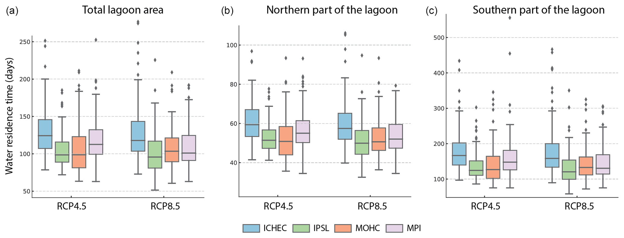
Figure A1Annual average water residence time (in days) in the total lagoon area (a) as well as separately for northern (b) and southern (c) parts of it under RCP4.5 and RCP8.5 scenarios.
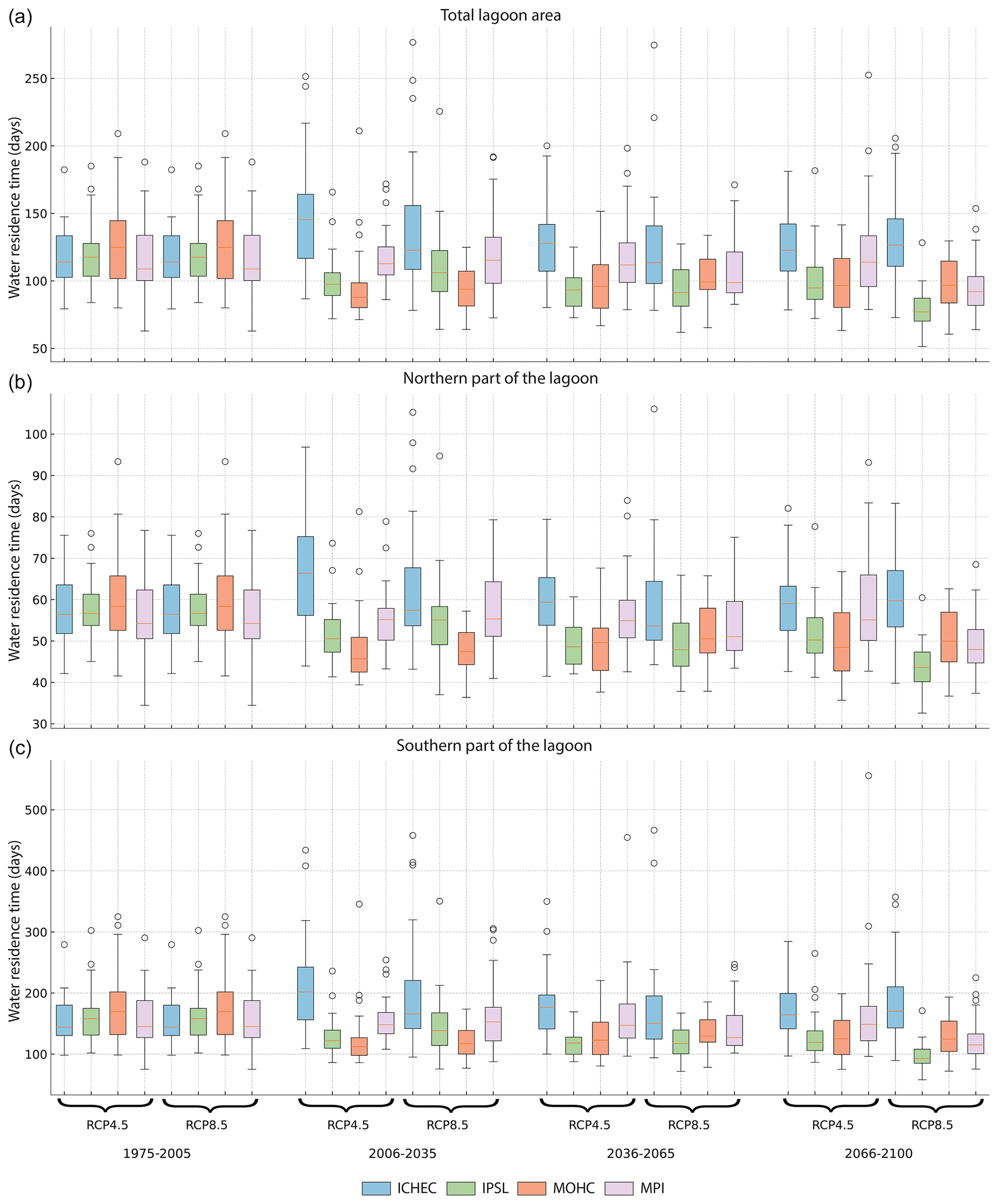
Figure A2Average water residence time (in days) in the total lagoon area (a) and northern (b) and southern parts (c) for RCP4.5 (left column) and RCP8.5 (right column) scenarios split into 30-year periods.
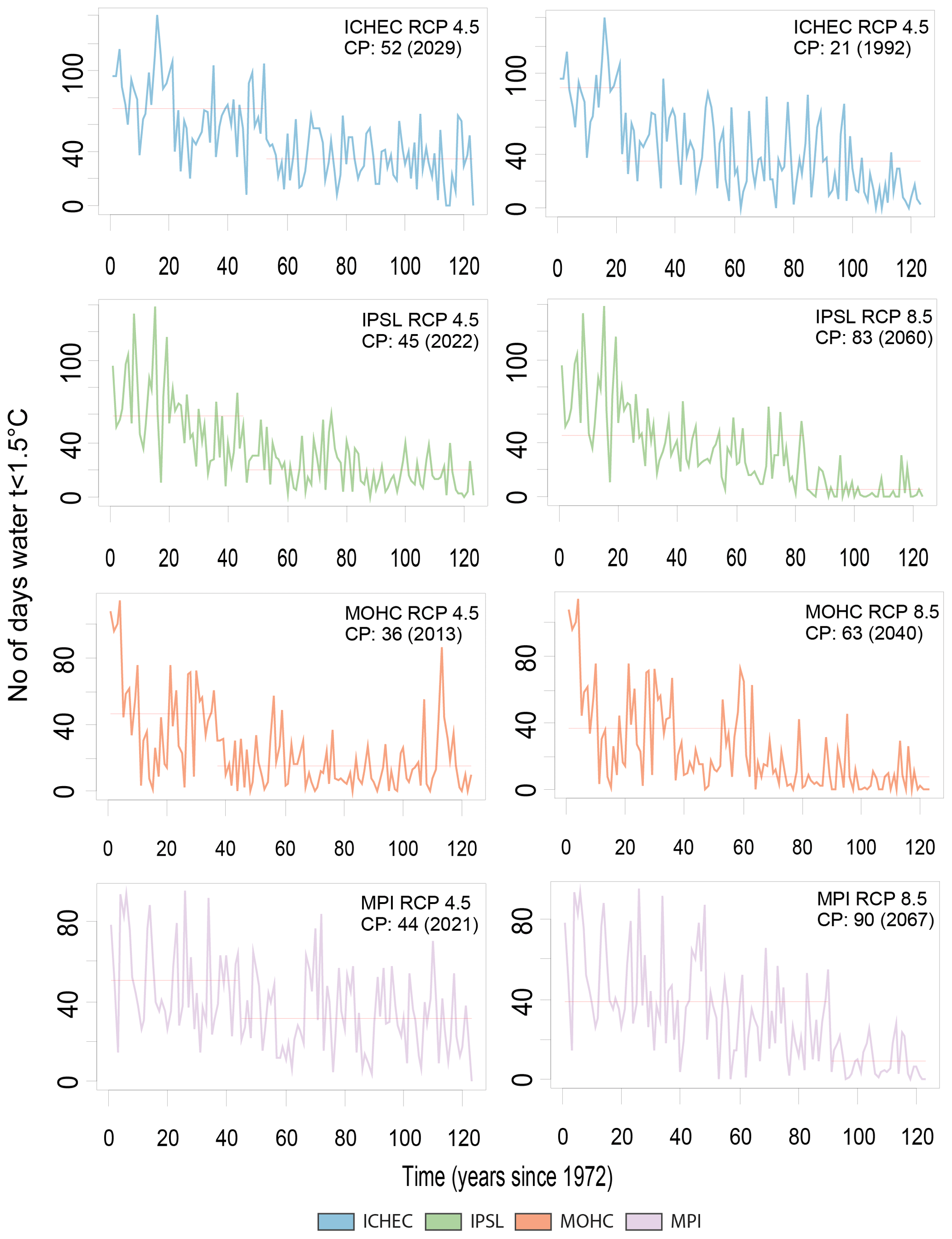
Figure B1Single changepoint (CP) detection in the modeled time series of the burbot spawning period for the duration of t<1.5 °C conditions (Vente area). Mean (M) and variance (V) of two periods are provided.
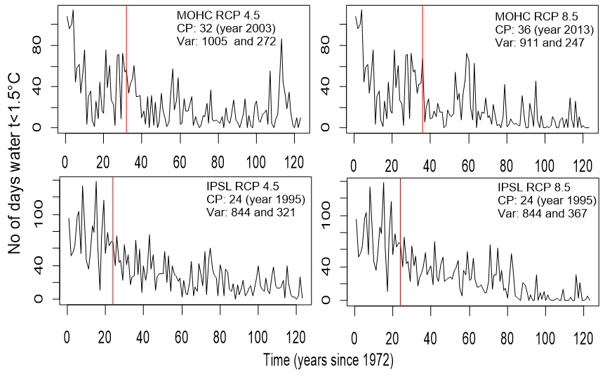
Figure B2Single changepoint (CP) of variance detection in the modeled time series of the burbot spawning period for the duration of t<1.5 °C conditions (Vente area). Variance (Var) of two periods is provided.
The Shallow water HYdrodynamic Finite Element Model (SHYFEM) software can be downloaded free of charge from the GitHub code repository (https://github.com/SHYFEM-model/, Umgiesser et al., 2024).
All numerical modeling results are openly available on the Zenodo open data repository (https://doi.org/10.5281/zenodo.7500744; Idzelytė et al., 2023b), initially generated in Idzelytė et al. (2023a) and cited in this paper.
GU and NC initiated the conceptualization and funding acquisition of the research project. NC, JM, and RI performed the analysis and drafted the paper. RI, NC, JM, and JL worked on the visualization of the results. NC, JM, and RI prepared the original manuscript draft with the assistance of JL, GU, and AE. All co-authors reviewed the paper and contributed to the scientific interpretation and discussion.
The contact author has declared that none of the authors has any competing interests.
Publisher's note: Copernicus Publications remains neutral with regard to jurisdictional claims made in the text, published maps, institutional affiliations, or any other geographical representation in this paper. While Copernicus Publications makes every effort to include appropriate place names, the final responsibility lies with the authors.
This project has received funding from the Research Council of Lithuania (LMTLT) (grant no. S-MIP-21-24).
This research has been supported by the Research Council of Lithuania (grant no. S-MIP-21-24).
This paper was edited by Mehmet Ilicak and reviewed by Mikolaj Piniewski and one anonymous referee.
Ashton, N. K., Jensen, N. R., Ross, T. J., Young, S. P., Hardy, R. S., and Cain, K. D.: Temperature and Maternal Age Effects on Burbot Reproduction, N. Am. J. Fish. Manage., 39, 1192–1206, https://doi.org/10.1002/nafm.10354, 2019.
Akstinas, V., Jakimavičius, D., Meilutytė-Lukauskienė, D., Kriaučiūnienė, J., and Šarauskienė, D.: Uncertainty of annual runoff projections in Lithuanian rivers under a future climate, Hydrol. Res., 51, 257–271, https://doi.org/10.2166/nh.2019.004, 2019.
Bartošová, A., Capell, R., Olesen, J. E., Jabloun, M., Refsgaard, J. C., Donnelly, C., Hyytiäinen, K., Pihlainen, S., Zandersen, M., and Arheimer, B.: Future socioeconomic conditions may have a larger impact than climate change on nutrient loads to the Baltic Sea, Ambio, 48, 1325–1336, https://doi.org/10.1007/s13280-019-01243-5, 2019.
Blöschl, G., Hall, J., Parajka, J., Perdigão, R. A. P., Merz, B., Arheimer, B., Aronica, G. T., Bilibashi, A., Bonacci, O., Borga, M., Čanjevac, I., Castellarin, A., Chirico, G. B., Claps, P., Fiala, K., Frolova, N., Gorbachova, L., Gül, A., Hannaford, J., Harrigan, S., Kireeva, M., Kiss, A., Kjeldsen, T. R., Kohnová, S., Koskela, J. J., Ledvinka, O., Macdonald, N., Mavrova-Guirguinova, M., Mediero, L., Merz, R., Molnar, P., Montanari, A., Murphy, C., Osuch, M., Ovcharuk, V., Radevski, I., Rogger, M., Salinas, J. L., Sauquet, E., Šraj, M., Szolgay, J., Viglione, A., Volpi, E., Wilson, D., Zaimi, K., and Živković, N.: Changing climate shifts timing of European floods, Science, 357, 588–590, https://doi.org/10.1126/science.aan2506, 2017.
Chen, C., Gan, R., Feng, D., Yang, F., and Zuo, Q.: Quantifying the contribution of SWAT modeling and CMIP6 inputting to streamflow prediction uncertainty under climate change, J. Clean. Prod., 364, 132675, https://doi.org/10.1016/j.jclepro.2022.132675, 2022.
Čerkasova, N., Umgiesser, G., and Ertürk, A.: Development of a hydrology and water quality model for a large transboundary river watershed to investigate the impacts of climate change – A SWAT application, Ecol. Eng., 124, 99–115, https://doi.org/10.1016/j.ecoleng.2018.09.025, 2018.
Čerkasova, N., Umgiesser, G., and Ertürk, A.: Assessing Climate Change Impacts on Streamflow, Sediment and Nutrient Loadings of the Minija River (Lithuania): A Hillslope Watershed Discretization Application with High-Resolution Spatial Inputs, Water, 11, 676, https://doi.org/10.3390/w11040676, 2019.
Čerkasova, N., Umgiesser, G., and Ertürk, A.: Modelling framework for flow, sediments and nutrient loads in a large transboundary river watershed: A climate change impact assessment of the Nemunas River watershed, J. Hydrol., 598, 126422, https://doi.org/10.1016/j.jhydrol.2021.126422, 2021.
Daggupati, P., Pai, N., Ale, S., Douglas-Mankin, K. R., Zeckoski, R. W., Jeong, J., Parajuli, P. B., Saraswat, D., and Youssef, M. A.: A recommended calibration and validation strategy for hydrologic and water quality models, T. ASABE, 58, 1705–1719, https://doi.org/10.13031/trans.58.10712, 2015.
Feyereisen, G. W., Strickland, T. C., Bosch, D. D., and Sullivan, D. G.: Evaluation of SWAT manual calibration and input parameter sensitivity in the Little River watershed, T. ASABE, 50, 843–855, 2007.
Foley, A.: Uncertainty in regional climate modeling: A review, Prog. Phys. Geog., 34, 647–670, https://doi.org/10.1177/0309133310375654, 2010.
Gupta, R., Bhattarai, R., and Mishra, A.: Development of Climate Data Bias Corrector (CDBC) Tool and Its Application over the Agro-Ecological Zones of India, Water, 11, 1102, https://doi.org/10.3390/w11051102, 2019.
Harrison, P. M., Gutowsky, L. F. G., Martins, E. G., Patterson, D. A., Cooke, S. J., and Power, M.: Temporal plasticity in thermal-habitat selection of burbot Lota lota a diel-migrating winter-specialist, Fish Biol., 88, 2095–2308, https://doi.org/10.1111/jfb.12990, 2016.
HELCOM: The revised nutrient input ceilings to the BSAP update, Helsinki Commission – HELCOM, https://helcom.fi/wp-content/uploads/2021/10/Nutrient-input-ceilings-2021.pdf (last access: 5 September 2024), 2021.
Hussain, M. and Mahmud, I.: pyMannKendall: a python package for nonparametric Mann Kendall family of trend tests, J. Open Source Softw., 4, 1556, https://doi.org/10.21105/joss.01556, 2019.
Idzelytė, R. and Umgiesser, G.: Application of an ice thermodynamic model to a shallow freshwater lagoon, Boreal Environ. Res., 26, 61–77, 2021.
Idzelytė, R., Mėžinė, J., Zemlys, P., and Umgiesser, G.: Study of ice cover impact on hydrodynamic processes in the Curonian Lagoon through numerical modeling, Oceanologia, 62, 428–442, https://doi.org/10.1016/j.oceano.2020.04.006, 2020.
Idzelytė, R., Čerkasova, N., Mėžinė, J., Dabulevičienė, T., Razinkovas-Baziukas, A., Ertürk, A., and Umgiesser, G.: Coupled hydrological and hydrodynamic modelling application for climate change impact assessment in the Nemunas river watershed–Curonian Lagoon–southeastern Baltic Sea continuum, Ocean Sci., 19, 1047–1066, https://doi.org/10.5194/os-19-1047-2023, 2023a.
Idzelytė, R., Čerkasova, N., Mėžinė, J., Dabulevičienė, T., Razinkovas-Baziukas, A., Ertürk, A., and Umgiesser, G.: The computation results of coupled hydrological and hydrodynamic modelling application for the Nemunas River watershed – Curonian Lagoon – South-Eastern Baltic Sea continuum, Zenodo [data set], https://doi.org/10.5281/zenodo.7500744, 2023b.
Inácio, M., Schernewski, G., Nazemtseva, Y., Baltranaitė, E., Friedland, R., and Benz, J.: Ecosystem services provision today and in the past: a comparative study in two Baltic lagoons, Ecol. Res., 33, 1255–1274, https://doi.org/10.1007/s11284-018-1643-8, 2018.
IPCC: Climate Change 2013: The Physical Science Basis. Contribution of Working Group I to the Fifth Assessment Report of the Intergovernmental Panel on Climate Change, edited by: Stocker, T. F., Qin, D., Plattner, G.-K., Tignor, M., Allen, S. K., Boschung, J., Nauels, A., Xia, Y., Bex, V., and Midgley, P. M., Cambridge University Press, Cambridge, United Kingdom and New York, NY, USA, 1535 pp., https://doi.org/10.1017/CBO9781107415324, 2013.
Ivanauskas, E., Skersonas, A., Andrašūnas, V., Elyaagoubi, S., and Razinkovas-Baziukas, A.: Mapping and Assessing Commercial Fisheries Services in the Lithuanian Part of the Curonian Lagoon, Fishes, 7, 19, https://doi.org/10.3390/fishes7010019, 2022.
Jakimavičius, D., Kriaučiūnienė, J., and Šarauskienė, D.: Impact of climate change on the Curonian Lagoon water balance components, salinity and water temperature in the 21st century, Oceanologia, 60, 378–389, https://doi.org/10.1016/j.oceano.2018.02.003, 2018.
Jakimavičius, D., Šarauskienė, D., and Kriaučiūnienė, J.: Influence of climate change on the ice conditions of the Curonian Lagoon, Oceanologia, 62, 164–172, https://doi.org/10.1016/j.oceano.2019.10.003, 2020.
Kaziukonytė, K., Lesutienė, J., Gasiūnaitė, Z. R., Morkūnė, R., Elyaagoubi, S., and Razinkovas-Baziukas, A.: Expert-Based Assessment and Mapping of Ecosystem Services Potential in the Nemunas Delta and Curonian Lagoon Region, Lithuania, Water, 13, 2728, https://doi.org/10.3390/w13192728, 2021.
Killick, R. and Eckley, I. A.: changepoint: An R Package for Changepoint Analysis, J. Stat. Softw., 58, 1–19, 2014.
Killick, R., Haynes, K., and Eckley, I. A.: changepoint: An R package for changepoint analysis, R package version 2.2.4, https://CRAN.R-project.org/package=changepoint (last access: 5 September 2024), 2022.
Latif, M.: Uncertainty in climate change projections, J. Geochem. Explor., 110, 1–7, https://doi.org/10.1016/j.gexplo.2010.09.011, 2011.
Lenderink, G., Buishand, A., and van Deursen, W.: Estimates of future discharges of the river Rhine using two scenario methodologies: direct versus delta approach, Hydrol. Earth Syst. Sci., 11, 1145–1159, https://doi.org/10.5194/hess-11-1145-2007, 2007.
Lehner, F., Deser, C., Maher, N., Marotzke, J., Fischer, E. M., Brunner, L., Knutti, R., and Hawkins, E.: Partitioning climate projection uncertainty with multiple large ensembles and CMIP5/6, Earth Syst. Dynam., 11, 491–508, https://doi.org/10.5194/esd-11-491-2020, 2020.
Lin, B., Chen, X., Yao, H., Chen, Y., Liu, M., Gao, L., and James, A.: Analyses of landuse change impacts on catchment runoff using different time indicators based on SWAT model, Ecol. Indic., 58, 55–63, https://doi.org/10.1016/j.ecolind.2015.05.031, 2015.
Lu, Y., Yuan, J., Lu, X., Su, C., Zhang, Y., Wang, C., Cao, X., Li, Q., Su, J., Ittekkot, V., Garbutt, R. A., Bush, S., Fletcher, S., Wagey, T., Kachur, A., and Sweijd, N.: Major threats of pollution and climate change to global coastal ecosystems and enhanced management for sustainability, Environ. Pollut., 239, 670–680, https://doi.org/10.1016/j.envpol.2018.04.016, 2018.
Madec, G. and NEMO System Team: NEMO ocean engine, Sci. Notes Clim. Model. Cent., 27, ISSN 1288-1619, Institut Pierre-Simon Laplace (IPSL), 2004.
Marotzke, J., Giering, R., Zhang, K. Q., Stammer, D., Hill, C., and Lee, T.: Construction of the adjoint MIT ocean general circulation model and application to Atlantic heat transport sensitivity, J. Geophys. Res.-Oceans, 104, 29529–29547, https://doi.org/10.1029/1999JC900236, 1999.
Meier, H. E. M., Kniebusch, M., Dieterich, C., Gröger, M., Zorita, E., Elmgren, R., Myrberg, K., Ahola, M. P., Bartosova, A., Bonsdorff, E., Börgel, F., Capell, R., Carlén, I., Carlund, T., Carstensen, J., Christensen, O. B., Dierschke, V., Frauen, C., Frederiksen, M., Gaget, E., Galatius, A., Haapala, J. J., Halkka, A., Hugelius, G., Hünicke, B., Jaagus, J., Jüssi, M., Käyhkö, J., Kirchner, N., Kjellström, E., Kulinski, K., Lehmann, A., Lindström, G., May, W., Miller, P. A., Mohrholz, V., Müller-Karulis, B., Pavón-Jordán, D., Quante, M., Reckermann, M., Rutgersson, A., Savchuk, O. P., Stendel, M., Tuomi, L., Viitasalo, M., Weisse, R., and Zhang, W.: Climate change in the Baltic Sea region: a summary, Earth Syst. Dynam., 13, 457–593, https://doi.org/10.5194/esd-13-457-2022, 2022a.
Meier, H. E. M., Dieterich, C., Gröger, M., Dutheil, C., Börgel, F., Safonova, K., Christensen, O. B., and Kjellström, E.: Oceanographic regional climate projections for the Baltic Sea until 2100, Earth Syst. Dynam., 13, 159–199, https://doi.org/10.5194/esd-13-159-2022, 2022b.
Mellor, G. L.: Users guide for a three-dimensional primitive equation numerical ocean model, Princeton Univ., Princeton, NJ, 08544–10710, 2004.
Neitsch, S. L., Arnold, J. G., Kiniry, J. R., and Williams, J. R.: Soil and Water Assessment Tool Theoretical Documentation Version 2009, Texas Water Resources Institute, College Station, Texas, https://swat.tamu.edu/media/99192/swat2009-theory.pdf (last access: 5 September 2024), 2009.
Plunge, S., Gudas, M., and Povilaitis, A.: Expected climate change impacts on surface water bodies in Lithuania, Ecohydrol. Hydrobiol., 22, 246–268, https://doi.org/10.1016/j.ecohyd.2021.11.004, 2022.
Rose, K. C., Bierwagen, B., Bridgham, S. D., Carlisle, D. M., Hawkins, C. P., Poff, N. L., Read, J. S., Rohr, J. R., Saros, J. E., and Williamson, C. E.: Indicators of the effects of climate change on freshwater ecosystems, Clim. Change, 176, 23, https://doi.org/10.1007/s10584-022-03457-1, 2023.
Song, Y. H., Chung, E. S., and Shiru, M. S.: Uncertainty Analysis of Monthly Precipitation in GCMs Using Multiple Bias Correction Methods under Different RCPs, Sustainability, 12, 7508, https://doi.org/10.3390/su12187508, 2020.
Shchepetkin, A. F. and McWilliams, J. C.: The regional oceanic modeling system (ROMS): a split-explicit, free-surface, topography-following-coordinate oceanic model, Ocean Model., 9, 347–404, https://doi.org/10.1016/j.ocemod.2004.08.002, 2005.
Stakėnienė, R., Jokšas, K., Kriaučiūnienė, J., Jakimavičius, D., and Raudonytė-Svirbutavičienė, E.: Nutrient Loadings and Exchange between the Curonian Lagoon and the Baltic Sea: Changes over the Past Two Decades (2001–2020), Water, 15, 4096, https://doi.org/10.3390/w15234096, 2023.
Stapanian, M. A., Paragamian, V. L., Madenjian, C. P., Jackson, J. R., Lappalainen, J., Evenson, M. J., and Neufeld, M. D.: Worldwide status of burbot and conservation measures, Fish Fish., 11, 34–56, https://doi.org/10.1111/j.1467-2979.2009.00340.x, 2010.
Švagždys, A.: Growth and abundance of burbot in the Curonian Lagoon and determinatives of burbot abundance, Acta Zool. Lit., 12, 58–64, https://doi.org/10.1080/13921657.2002.10512487, 2002.
Taylor, K. E., Stouffer, R. J., and Meehl, G. A.: An Overview of CMIP5 and the Experiment Design, B. Am. Meteorol. Soc., 93, 485–498, https://doi.org/10.1175/bams-d-11-00094.1, 2012.
Tedesco, L., Vichi, M., Haapala, J., and Stipa, T.: An enhanced sea-ice thermodynamic model applied to the Baltic Sea, Boreal Environ. Res., 14, 68–80, 2009.
Tegegne, G., Melesse, A. M., and Worqlul, A. W.: Development of multi-model ensemble approach for enhanced assessment of impacts of climate change on climate extremes, Sci. Total Environ., 704, 135357, https://doi.org/10.1016/j.scitotenv.2019.135357, 2020.
Umgiesser, G., Melaku Canu, D., Cucco, A., and Solidoro, C.: A finite element model for the Venice Lagoon. Development, set up, calibration and validation, J. Mar. Syst., 51, 123–145, https://doi.org/10.1016/j.jmarsys.2004.05.009, 2004.
Umgiesser, G., Ferrarin, C., Cucco, A., De Pascalis, F., Bellafiore, D., Ghezzo, M., and Bajo, M.: Comparative hydrodynamics of 10 Mediterranean lagoons by means of numerical modeling, J. Geophys. Res.-Oceans, 119, 2212–2226, https://doi.org/10.1002/2013JC009512, 2014.
Umgiesser, G., Zemlys, P., Erturk, A., Razinkova-Baziukas, A., Mėžinė, J., and Ferrarin, C.: Seasonal renewal time variability in the Curonian Lagoon caused by atmospheric and hydrographical forcing, Ocean Sci., 12, 391–402, https://doi.org/10.5194/os-12-391-2016, 2016.
Umgiesser, G., Ferrarin, C., Bajo, M., Laurent, C., shyfem-cm, Arpaia, L., fivan, Pinsky, A., Ghezzo, M., Chegini, T., dbellafiore, and jalessandri: SHYFEM, https://github.com/SHYFEM-model/, GitHub [code], 2024.
Viitasalo, M. and Bonsdorff, E.: Global climate change and the Baltic Sea ecosystem: direct and indirect effects on species, communities and ecosystem functioning, Earth Syst. Dynam., 13, 711–747, https://doi.org/10.5194/esd-13-711-2022, 2022.
Vybernaite-Lubiene, I., Zilius, M., Saltyte-Vaisiauske, L., and Bartoli, M.: Recent Trends (2012–2016) of N, Si, and P Export from the Nemunas River Watershed: Loads, Unbalanced Stoichiometry, and Threats for Downstream Aquatic Ecosystems, Water, 10, 1178, https://doi.org/10.3390/w10091178, 2018.
Waikhom, S. I., Yadav, V., Azamathulla, H. M., and Solanki, N.: Impact assessment of land use/land cover changes on surface runoff characteristics in the Shetrunji River Basin using the SWAT model, Water Pract. Tech., 18, 1221–1232, https://doi.org/10.2166/wpt.2023.071, 2023.
Wang, G., Yang, H., Wang, L., Xu, Z., and Xue, B.: Using the SWAT model to assess impacts of land use changes on runoff generation in headwaters, Hydrol. Process., 28, 1032–1042, https://doi.org/10.1002/hyp.9645, 2012.
Zemlys, P., Ferrarin, C., Umgiesser, G., Gulbinskas, S., and Bellafiore, D.: Investigation of saline water intrusions into the Curonian Lagoon (Lithuania) and two-layer flow in the Klaipėda Strait using finite element hydrodynamic model, Ocean Sci., 9, 573–584, https://doi.org/10.5194/os-9-573-2013, 2013.
- Abstract
- Introduction
- Materials and methods
- Results
- Discussion
- Conclusions and recommendations
- Appendix A: Additional results of the water residence time
- Appendix B: Results of the changepoint analysis
- Code availability
- Data availability
- Author contributions
- Competing interests
- Disclaimer
- Acknowledgements
- Financial support
- Review statement
- References