Validating the spatial variability in the semidiurnal internal tide in a realistic global ocean simulation with Argo and mooring data

The autocovariance of the semidiurnal internal tide (IT) is examined in a 32 d segment of a global run of the HYbrid Coordinate Ocean Model (HYCOM). This numerical simulation, with 41 vertical layers and $\mathrm{1}/\mathrm{25}$^∘ horizontal resolution, includes tidal and atmospheric forcing, allowing for the generation and propagation of ITs to take place within a realistic eddying general circulation. The HYCOM data are in turn compared with global observations of the IT around 1000 dbar, from Argo float park-phase data and mooring records. HYCOM is found to be globally biased low in terms of the IT variance and decay of the IT autocovariance over timescales shorter than 32 d. Except in the Southern Ocean, where limitations in the model cause the discrepancy with in situ measurements to grow poleward, the spatial correlation between the Argo and HYCOM tidal variance suggests that the generation of low-mode semidiurnal ITs is globally well captured by the model.

1 Introduction

Internal tides (ITs) are internal waves generated by the interaction of tidal currents with rough bathymetry. The radiated wave beams can travel thousands of kilometers (e.g., Zhao et al., 2016; Buijsman et al., 2020), over which they undergo dissipative processes as they interact with the eddying ocean and bottom topography to eventually break (MacKinnon et al., 2017). The dissipation of ITs represents a major source of vertical mixing in the ocean interior (de Lavergne et al., 2020). As such, ITs have a key influence on the ocean state (Melet et al., 2016) and therefore on the global climate system (see Melet et al., 2022, for a review on the subject).

At any given position in a stationary medium, tidally forced waves would have a constant phase difference to the astronomical forcing. However, since they propagate within the time-varying ocean circulation, ITs are subject to a variety of mechanisms that cause their phase difference to the tidal forcing at their generation site to shift with time (Rainville and Pinkel, 2006; Shriver et al., 2014; Zaron and Egbert, 2014; Buijsman et al., 2017). In other words, ITs lose coherence by interacting with the eddying ocean. They decorrelate: the autocovariance of a time series representing the internal tide variability at a fixed position (away from the source) inevitably decays with time lag (Caspar-Cohen et al., 2022; Geoffroy and Nycander, 2022).

Only the coherent fraction of the IT energy decays with time lag, that is the energy carried by waves with a constant phase difference to the astronomical forcing. Conversely, the incoherent fraction of the energy grows so that the total IT energy, or variance, at a given location (the sum of the coherent and incoherent components) is unaffected by the decorrelation. For very long time lags, the coherent and the complementary incoherent asymptotic limits are often called stationary and nonstationary variance, respectively. While the global field of the stationary (low-mode) IT is widely considered to be well constrained by multiyear satellite altimetry observations (Dushaw et al., 2011; Ray and Zaron, 2016; Zaron, 2019; Zhao, 2019), the nonstationary component is not.

Some current high-resolution global ocean circulation models enable the estimation of the barotropic and internal tides concurrently with the ocean circulation (Arbic et al., 2010; Shriver et al., 2012; Buijsman et al., 2020). Such fully nonlinear numerical simulations also incorporate the interactions of the generated ITs with the eddying ocean and its boundaries. The model utilized in this study is the HYbrid Coordinate Ocean Model (HYCOM; Chassignet et al., 2006), with 41 vertical layers and $\mathrm{1}/\mathrm{25}$^∘ horizontal resolution. The literature on the validation of HYCOM with observations is already vast (see Buijsman et al., 2020, and Arbic, 2022, for recent accounts). In the latest developments, surface drifters have been used to validate the geographical variability in the kinetic energy in various frequency bands at the global scale (Arbic et al., 2022). While the global coverage of drifter data is comparable to that of satellite altimetry, the contribution from the baroclinic tides to the kinetic energy observed by drifters has not been determined yet. Hence, until recently, only altimetry could unveil the geographical variability in the ITs at the global scale.

The empirical mapping of ITs from altimetry remains challenging for various reasons (Egbert and Ray, 2017). Most notably, the long sampling intervals of altimeters and the low signal-to-noise ratio preclude any direct estimation in the time domain of the total IT variance at a single location. Notwithstanding, Zaron (2017) analyzed along-track wavenumber spectra of the sea surface height to map the total and nonstationary semidiurnal IT variance (for the baroclinic mode 1 only). The author found a global-mean ratio of nonstationary to total semidiurnal IT variance of 44 %. He also outlined the spatial inhomogeneity of the tidal variability, with this ratio being larger than 50 % in much of the equatorial Pacific and Indian oceans (Zaron, 2017). In a comparison with data from HYCOM, Nelson et al. (2019) showed the “k-space” methodology of Zaron (2017) to miss a large fraction of both the nonstationary and total variance. Nevertheless, the spatial correlation of the nonstationary fraction (i.e., the ratio of the nonstationary to total variance) between the model and altimetry suggests that the model at least qualitatively captures the generation of ITs and their interactions with the background circulation (Nelson et al., 2019).

Recently, Geoffroy and Nycander (2022) used observations from Argo park-phase data (Argo, 2000) to empirically map the variance of the semidiurnal IT at 1000 dbar. The high sampling rate of the floats captures the total variance of the IT, i.e., the autocovariance at short time lags, before any significant loss of coherence occurs and after most of the noise has decorrelated. On the other hand, the Lagrangian sampling of the drifting floats results in decorrelating effects on top of the decorrelation of the IT itself (Zaron and Elipot, 2021; Caspar-Cohen et al., 2022; Geoffroy and Nycander, 2022). Following Caspar-Cohen et al. (2022), we call the effects of the Lagrangian sampling on the autocovariance apparent decorrelation. This apparent decorrelation cannot be disentangled from the decorrelation of the IT (i.e., the decorrelation due to interactions with the background circulation) using Argo data only. Thus, to gain insights into the IT decorrelation around 1000 dbar, one can instead apply the methodology of Geoffroy and Nycander (2022) to Eulerian observations from moorings. In the present work we compare observations of the (total) variance and decorrelation of the semidiurnal IT around 1000 dbar from Argo floats and moorings, respectively, to data from a global HYCOM run. Contrarily to other recent validations of HYCOM with mooring data (e.g., Ansong et al., 2017; Luecke et al., 2020), the Eulerian component of our analysis is not meant as a standalone point-to-point comparison. Rather, it is designed to bolster and extend the main analysis of the Lagrangian data.

The remainder of this work is organized as follows: in Sect. 2, the in situ datasets and the numerical simulation are presented. In Sect. 3, we review the methodology of Geoffroy and Nycander (2022) in an example location from the Lagrangian and Eulerian perspectives. In Sect. 4, the main results are presented. We compare the geographical variability in the variance and decorrelation of the semidiurnal IT obtained from the in situ data and numerical simulation. Then, the model data are used to quantify the decorrelation induced by the Lagrangian sampling. Finally, we outline the potential biases affecting the datasets. We conclude in Sect. 5 by discussing the results and giving a summary.

2 Data

The different comparisons in this work are all done in terms of vertical displacement of the isotherms. The measurable variables needed to compute vertical isotherm displacement at a fixed depth are the temperature anomaly and vertical temperature gradient at that depth. In this section we briefly describe the temperature time series from each dataset.

2.1 Argo floats with Iridium communication

We use data from a global collection of Argo Iridium floats deployed by the University of Washington as part of the National Ocean Partnership Program during the period 2004–2022. Between the descending and ascending profiling phases, these floats also record temperature and pressure with an hourly resolution while adrift at 1000 dbar. This so-called park phase typically lasts 10 d. As in Hennon et al. (2014) and Geoffroy and Nycander (2022), we use the pressure records to correct for the small departures of a float from its drifting control level during a park phase.

Stitching together data from successive cycles, by filling the time between park phases (typically 6 h) with NaN (not a number) values, one can construct longer time series. In this study, we use segments of 32 d of data (i.e., the duration of the segment of numerical simulation we are using). The sampling period of the park phase can occasionally vary by more than a few seconds. To ensure evenly spaced time series, we linearly interpolate each concatenated record of 32 d onto a time axis with a constant 1 h step. Any interpolated value lying between two original records that are more than 1.5 h apart is replaced by NaN.

The position of the floats can only be determined when they reach the surface. We assume straight trajectories between two successive surfacings (typically 10 d apart). This assumption has been shown to be reasonable by Geoffroy and Nycander (2022), especially since we discard segments of data for which the mean speed of the float is larger than 0.1 m s⁻¹. This criterion is primarily intended to avoid contamination by lee waves: a flow with speed U≈0.1 m s⁻¹ passing over a bathymetric feature with horizontal length scale λ≈10 km will generate lee waves with angular frequency $\mathit{\omega }=(\mathrm{2}\mathit{\pi }/\mathit{\lambda })U$ rad s⁻¹ of the order of the diurnal frequency.

The Argo dataset used in this work is an updated version of the one used by Geoffroy and Nycander (2022). After the base processing and quality controls, we are left with 22 414 valid 32 d segments from 891 individual floats. A more detailed description of the Argo data processing and quality controls we employed is available from Hennon et al. (2014) and Geoffroy and Nycander (2022).

2.2 Global Multi-Archive Current Meter Database (GMACMD)

The Global Multi-Archive Current Meter Database (GMACMD; Scott et al., 2011) compiles tens of thousands of oceanographic time series from moorings. Previous model–data validation efforts involving both HYCOM and mooring data notably include Luecke et al. (2020), where the authors compared the temperature variance and kinetic energy over various frequency bands in realistic global ocean simulations to more than 3800 instrumental records.

Here, we extracted 331 temperature time series spanning 1972–2010 and meeting the following criteria:

1. The mooring lies in water deeper than 2000 m.

2. The record is longer than 64 d, with a sampling interval shorter than 3 h, for adequate resolution of the semidiurnal tidal signals.

3. The instrument depth is within ±200 from 1000 m.

One particular mooring is used as an example in Sect. 3. It recorded during 366 d in the years 1982–1983 at the position 28.00^∘ N, 151.95^∘ W (north of the Hawaiian Ridge). As previously documented by Alford and Zhao (2007), we refer to the instrument at 1119 m depth as mooring no. 2. This instrument sampled temperature with a 0.25 h resolution.

2.3 HYbrid Coordinate Ocean Model (HYCOM)

This study uses 32 d, from 20 May to 20 June 2019, of hourly output at 1000 m depth from a global run of HYCOM, with 41 vertical layers and $\mathrm{1}/\mathrm{25}$^∘ horizontal resolution. The non-data-assimilative simulation, designated “GLBy190.04”, includes realistic tidal and atmospheric forcing enabling the generation and propagation of ITs within the eddying general circulation. The high-resolution 2D fields are complemented by monthly mean 3D fields of temperature and salinity subsampled to 1^∘.

A Lagrangian analysis of the simulation is used for a direct model–data validation with Argo floats. The Argo quasi-Lagrangian sampling is mimicked by releasing 41 644 particles randomly across the world oceans. We let the particles be advected by the 2D velocity field at 1000 m for 32 d while sampling temperature with an hourly resolution. This Lagrangian sampling of HYCOM is achieved using the software Parcels (Van Sebille et al., 2021). The Lagrangian simulation uses a classic Runge–Kutta method for computing the advection of the particles (with 5 min integration time step). As for the Argo data, we discard particles with a mean speed larger than 0.1 m s⁻¹. We also discard any particle crossing the 1000 m isobath during the simulation.

3 Methods

In this section, we present a local example to introduce the methods that are used in Sect. 4 for the global comparison. We start by comparing the Argo observations to the Lagrangian sampling of the HYCOM data. Next, we investigate the effects of the drift by comparing Lagrangian and Eulerian samplings of the numerical simulation. We end the section by introducing the comparison between the Eulerian HYCOM time series and mooring observations.

3.1 Lagrangian sampling of the isopycnal displacement at 1000 dbar

As in Hennon et al. (2014) and Geoffroy and Nycander (2022), we define the vertical isotherm displacement observed by a Lagrangian particle ${\mathit{\eta }}_{\mathrm{1000}}^{\mathrm{L}}$ as

$$\begin{array}{}\text{(1)}& {\mathit{\eta }}_{\mathrm{1000}}^{\mathrm{L}}\left(t\right)={\displaystyle \frac{T\left(t\right)-\stackrel{\mathrm{‾}}{T}}{(\mathrm{d}T/\mathrm{d}P{)}_{\mathrm{1000}}(t)}},\end{array}$$

where $\stackrel{\mathrm{‾}}{T}$ is the time average of the temperature measurements T(t) over a particle trajectory, and $(\mathrm{d}T/\mathrm{d}P{)}_{\mathrm{1000}}(t)$ is the temperature gradient at 1000 dbar. Hence, the vertical isotherm displacement is simply computed as the temperature anomaly recorded by a drifting particle at 1000 dbar divided by the vertical temperature gradient at that depth. For HYCOM particles, we compute $(\mathrm{d}T/\mathrm{d}P{)}_{\mathrm{1000}}$ as the mean, between 900 and 1100 m, of the vertical gradient calculated from the modeled monthly mean 3D temperature field. We then linearly interpolate the temperature gradient in the horizontal to the successive particle positions (hence the time dependence). To avoid any spurious displacements, we set ${\mathit{\eta }}_{\mathrm{1000}}^{\mathrm{L}}$ to NaN whenever the magnitude of the temperature gradient is smaller than $\mathrm{3}\times {\mathrm{10}}^{-\mathrm{5}}$ ^∘C dbar⁻¹.

In the case of Argo floats, Eq. (1) is evaluated over each park phase. $\stackrel{\mathrm{‾}}{T}$ then represents the time average of the temperature measurements T(t) over a park phase, and the vertical temperature gradient is estimated from the average of the two neighboring ascending profiles. Specifically, $(\mathrm{d}T/\mathrm{d}P{)}_{\mathrm{1000}}(t)$ is computed as the mean, within 100 dbar of the parking pressure, of the vertical gradient calculated from the average temperature profile. As for the HYCOM particles, we discarded the data from the whole park phase whenever the magnitude of the temperature gradient is smaller than $\mathrm{3}\times {\mathrm{10}}^{-\mathrm{5}}$ ^∘C dbar⁻¹. As explained in Sect. 2.1, ${\mathit{\eta }}_{\mathrm{1000}}^{\mathrm{L}}$ time series from successive park phases are stitched together to constitute 32 d time series.

For both Argo floats and HYCOM Lagrangian particles, the low-frequency background activity is filtered out from ${\mathit{\eta }}_{\mathrm{1000}}^{\mathrm{L}}$ using a fourth-order Butterworth filter with a cut-off frequency of 0.3 cpd (cycles per day). The inertial peak is not removed by this filter poleward of about ±10^∘ latitude.

3.2 Averaging sample autocovariance series

The HYCOM-derived Lagrangian time series ${\mathit{\eta }}_{\mathrm{1000}}^{\mathrm{L}}$ can be analyzed in the same way as in Geoffroy and Nycander (2022). We illustrate the mapping process below. The geographical patch presented here is also described in Geoffroy and Nycander (2022). For this example area, Fig. 1 shows eight 32 d segments of Argo data and 13 HYCOM particles selected using their median position. The circular patch of 200 km radius containing the latter median positions is centered on mooring no. 2.

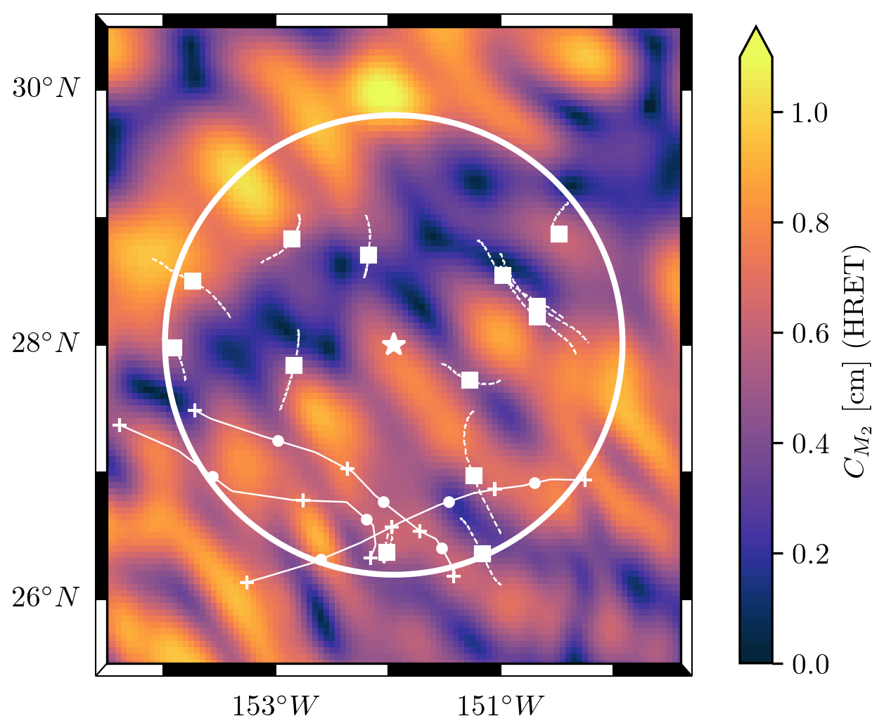
Figure 1 Example circular geographical patch of 200 km radius (the white star denotes mooring no. 2 at the center). The median positions of the segments of Argo data and of the HYCOM particles are shown by white filled circles and white squares, respectively. The dashed white curves represent the trajectories of the HYCOM particles over the 32 d of numerical simulation. The binned Argo segments were all recorded by the same float; its trajectory is shown by the solid white curve, with white crosses denoting the starting and ending points of the different 32 d segments. In the background we show the amplitude of the M₂ baroclinic sea level anomaly from the High Resolution Empirical Tide model (HRET; Zaron, 2019).

From a finite time series η(t) one can calculate the sample autocovariance $\widehat{R}\left(\mathit{\tau }\right)$:

$$\begin{array}{}\text{(2)}& \widehat{R}\left(\mathit{\tau }\right)={\displaystyle \frac{\mathrm{1}}{N-\mathit{\tau }}}\sum _{t=\mathrm{1}}^{N-\mathit{\tau }}({\mathit{\eta }}_t-\widehat{\stackrel{\mathrm{‾}}{\mathit{\eta }}})({\mathit{\eta }}_{t+\mathit{\tau }}-\widehat{\stackrel{\mathrm{‾}}{\mathit{\eta }}}),\end{array}$$

where N is the total number of observations, and $\widehat{\stackrel{\mathrm{‾}}{\mathit{\eta }}}$ is the sample mean of the series. Note that $\widehat{R}\left(\mathrm{0}\right)$ is the sample variance of the series. Here, N is taken as the number of non-missing observations, accounting for gaps in the Argo time series (during the descent, main profiling, and surface transmission phases of the float cycle or because of failed quality controls). The sample autocovariance as defined in Eq. (2) is an unbiased estimator of the “true” autocovariance (i.e., $\widehat{R}\left(\mathit{\tau }\right)$ converges to the true value R(τ) for infinitely large N). In the remainder of this article we only compute the variance and autocovariance of vertical isotherm displacement time series. For the sake of brevity, we simply refer to them as the variance and autocovariance.

The sample autocovariances for all HYCOM particles within the circular patch shown in Fig. 1 are averaged to obtain a local-mean autocovariance ${\stackrel{\mathrm{‾}}{R}}_{\mathrm{HYCOM}}^{\mathrm{L}}$. The local-mean autocovariance from the Argo data, ${\stackrel{\mathrm{‾}}{R}}_{\mathrm{Argo}}$, is computed in the same way. The standard error of the local-mean autocovariance is computed as

$$\begin{array}{}\text{(3)}& \mathrm{SEM}\left(\mathit{\tau }\right)={\displaystyle \frac{\mathrm{STD}\left(\mathit{\tau }\right)}{\sqrt{N_{\mathrm{p}}}}},\end{array}$$

where STD is the standard deviation of the sample autocovariances over the subset, and N_p is the number of particles in the subset. Figure 2a demonstrates the good agreement of the two datasets until τ≈200 h. Past this time lag limit, ${\stackrel{\mathrm{‾}}{R}}_{\mathrm{Argo}}$ falls under its 95 % confidence interval (95 % C.I. = ±2 SEM) and thus cannot be considered significantly different from zero.

A handy tool for monitoring the evolution of the autocovariance of the semidiurnal IT is complex demodulation. Here, it consists of the least squares fitting of Acos (ω_SDτ)+Bsin (ω_SDτ), where ${\mathit{\omega }}_{\mathrm{SD}}=({\mathit{\omega }}_{{\mathrm{M}}_{\mathrm{2}}}+{\mathit{\omega }}_{{\mathrm{S}}_{\mathrm{2}}})/\mathrm{2}$ is the semidiurnal frequency, to the sample autocovariance in 48 h windows with 75 % overlap. This is equivalent to fitting Ccos (ω_SDτ+Φ), where C and Φ are the amplitude and phase, respectively. We then define the complex demodulate as $C=\sqrt{A^{\mathrm{2}}+B^{\mathrm{2}}}$. This positive definite amplitude follows the envelope of the modulated sinusoidal with frequency ω_SD. Note that this definition differs from the complex demodulation used in Geoffroy and Nycander (2022), where the authors fitted Ccos (ω_SDτ), i.e., with Φ=0. In practice, we compute the complex demodulate of the autocovariance following the harmonic analysis method of Cherniawsky et al. (2001). The demodulation over a given 48 h window is performed in two iterations. We first fit Acos (ω_SDτ)+Bsin (ω_SDτ) to the signal and compute the root mean square error (RMSE). We then repeat the fitting with a trimmed signal that excludes values outside of ±2 RMSE from the previously fitted curve.

Complex demodulation is just a convenient way of finding the envelope of the sample estimate of an underlying true oscillating function at a given frequency. However, as an estimate of the envelope of the true oscillating function, the complex demodulate can be shown to be biased high (see Appendix A). This bias is greatly mitigated (i) at short time lags and (ii) when the sample size is large (e.g., when demodulating regional- or global-mean autocovariances). Throughout this paper we only rely on complex demodulation in one case or the other. A conservative estimate of the uncertainty in the envelope of the sample function (i.e., the uncertainty in the demodulate) is the uncertainty in the sample function itself. If this uncertainty range is larger than the envelope of the sample function, the conclusion is not that the envelope of the true function can be negative but that it is not significantly different from zero. Here, we evaluate the uncertainty affecting the complex demodulate of a mean autocovariance series over a 48 h window by computing the median of the standard error over that window, hereinafter denoted $\stackrel{\mathrm{̃}}{\mathrm{SEM}}$. The corresponding 95 % confidence intervals are taken as $\pm \mathrm{2}\stackrel{\mathrm{̃}}{\mathrm{SEM}}$.

Following Geoffroy and Nycander (2022), the semidiurnal IT variance can be estimated from the first 48 h demodulate at the semidiurnal frequency. In Appendix B we investigate the potential contamination of the first demodulate by the non-tidal variability (noise). We found that a background noise can contribute either positively or negatively (a consequence of filtering the time series) to the amplitude of the first demodulate, depending on its characteristic timescale. Notwithstanding, for a typical signal-to-noise ratio and timescale of the background noise observed by Argo floats, the first demodulate was seen to remain a conservative estimate of the IT variance. The effects of the non-tidal variability on the IT variance estimate as computed in Geoffroy and Nycander (2022) thus do not put their results into question.

Since HYCOM does not resolve the full spectrum of the oceanic variability, in particular the variability associated with short timescales, the corresponding stochastic noise is expected to differ from the one captured by the in situ data (in terms of both variance and characteristic timescale). The contamination of the first demodulate by this noise would therefore account for a systematic bias when comparing the simulated data with observations. To limit this, we chose to consistently subtract an estimate of the autocovariance of the non-tidal variability from the sample mean autocovariance before computing the complex demodulates. The way we obtain such an estimate is described in Appendix C. Namely, we fit a model of the autocovariance of a tidal variability on top of a background noise to the sample autocovariance by nonlinear least squares. Besides the noise parameters, this also provides us with an estimate of the tidal variance. Still, in this work, we chose to perform the comparisons in terms of the first demodulate for it is a conservative and more robust estimate of the IT variance.

The result of the complex demodulation at the semidiurnal frequency applied to our two (noise-corrected) mean autocovariance series is presented in Fig. 2b. The first 48 h complex demodulate is taken as a direct estimate of the semidiurnal IT variance. From the Argo data plotted in Fig. 2b we obtain 24.9 m², with a 95 % C.I. of [16.7, 33.2] m². For this local example, the first demodulate of ${\stackrel{\mathrm{‾}}{R}}_{\mathrm{HYCOM}}^{\mathrm{L}}$ is almost identical to the first demodulate of ${\stackrel{\mathrm{‾}}{R}}_{\mathrm{Argo}}$. Apart from the first couple of demodulates, the HYCOM demodulate series appears consistently smaller than the Argo one.

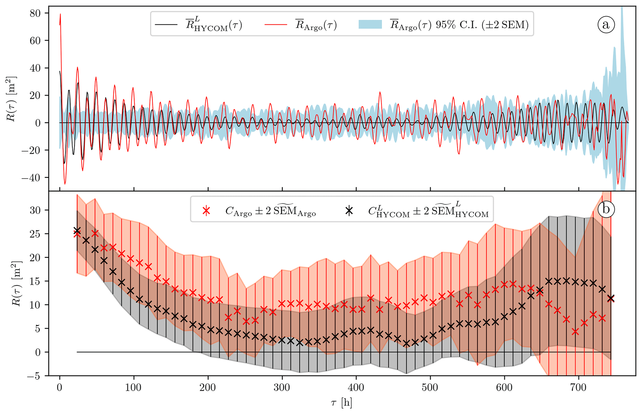
Figure 2 (a) Local-mean autocovariance ${\stackrel{\mathrm{‾}}{R}}_{\mathrm{HYCOM}}^{\mathrm{L}}$ computed from the HYCOM particles (solid black curve) and local-mean autocovariance ${\stackrel{\mathrm{‾}}{R}}_{\mathrm{Argo}}$ computed from the 32 d segments of Argo data (solid red curve) and 95 % confidence interval of ${\stackrel{\mathrm{‾}}{R}}_{\mathrm{Argo}}$ (light-blue shading). The data are from the geographical patch shown in Fig. 1. (b) Complex demodulates at the semidiurnal frequency of the autocovariance series shown in (a) and their 95 % C.I. The red and gray shadings highlight the 95 % C.I. for the Argo and Lagrangian HYCOM data, respectively.

3.3 Eulerian perspective

The decay with time lag of the demodulates represented as red crosses in Fig. 2b mirrors the decorrelation captured by the Lagrangian sampling of the Argo floats. The motion of the instruments results in decorrelating effects that cannot be isolated from the loss of coherence of the IT. However, by analyzing the HYCOM data within a Eulerian framework, one can directly monitor the decorrelation of the IT. The Eulerian HYCOM time series can then be compared with observations from moorings.

In the Eulerian framework, our methods remain practically unchanged. We now define the vertical isotherm displacement at a given location as

$$\begin{array}{}\text{(4)}& {\mathit{\eta }}_{\mathrm{1000}}^{\mathrm{E}}(x,y,t)={\displaystyle \frac{T(x,y,t)-\stackrel{\mathrm{‾}}{T}(x,y)}{(\mathrm{d}T/\mathrm{d}P{)}_{\mathrm{1000}}(x,y)}},\end{array}$$

where $\stackrel{\mathrm{‾}}{T}(x,y)$ is the time average of the temperature field $T(x,y,t)$, and $(\mathrm{d}T/\mathrm{d}P{)}_{\mathrm{1000}}(x,y)$ is the temperature gradient at 1000 m, calculated from the modeled monthly mean 3D temperature field. As for the Lagrangian time series, we apply a fourth-order Butterworth high-pass filter with a cut-off frequency of 0.3 cpd on ${\mathit{\eta }}_{\mathrm{1000}}^{\mathrm{E}}$.

For each HYCOM particle, we compute 32 d long time series of ${\mathit{\eta }}_{\mathrm{1000}}^{\mathrm{E}}$ at the successive positions of the particle subsampled at a 12 h rate. We then calculate the sample autocovariance from each of these time series and average the results over the particle's trajectory. As in the Lagrangian framework, the resulting averages can be averaged over different particles to compute local- and global-mean autocovariance series. By estimating the Eulerian autocovariance along the Lagrangian trajectories we account for the geographic variability in the IT. Also, our Eulerian sample autocovariance estimates contain many more degrees of freedom than their Lagrangian equivalents. As a result, the uncertainty affecting the Eulerian autocovariance estimates is much smaller.

Equation (4) is also used to compute vertical displacement time series from the mooring temperature records. Here, the vertical temperature gradient is computed from the annual-mean climatology (WOA18; Boyer et al., 2018) as an average of the temperature gradient within 100 m of the instruments' depth. As for the HYCOM and Argo data, we discarded instruments for which the magnitude of the temperature gradient is smaller than $\mathrm{3}\times {\mathrm{10}}^{-\mathrm{5}}$ ^∘C dbar⁻¹. Each mooring time series is split into successive 32 d segments. We then compute the sample autocovariance for each high-pass-filtered segment and average them to obtain a mean autocovariance.

The Eulerian sampling serves two main purposes: (i) validating the variance of the IT measured by the Lagrangian particles and (ii) comparing the decorrelation of the IT in the HYCOM data with mooring observations. We illustrate these two aspects for the local example introduced in Sect. 3.2 in Figs. 3 and 4, respectively.

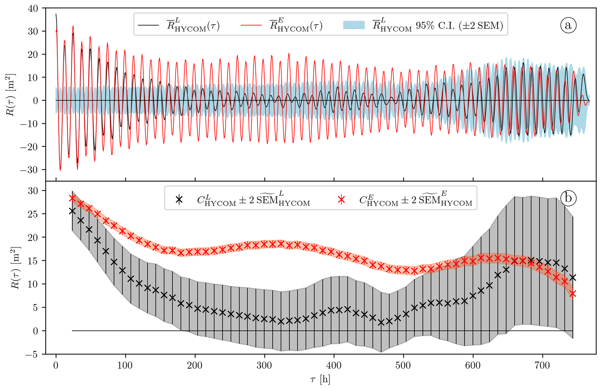
Figure 3 (a) Mean autocovariance computed from ${\mathit{\eta }}_{\mathrm{1000}}^{\mathrm{L}}$ (solid black curve, same as the solid black curve in Fig. 2a) and 95 % confidence interval of ${\stackrel{\mathrm{‾}}{R}}_{\mathrm{HYCOM}}^{\mathrm{L}}$ (light-blue shading) and mean autocovariance computed from ${\mathit{\eta }}_{\mathrm{1000}}^{\mathrm{E}}$ (solid red curve). The data are from the geographical patch shown in Fig. 1. (b) Complex demodulates at the semidiurnal frequency of the autocovariance series shown in (a) and their 95 % C.I. The red and gray shadings highlight the 95 % C.I. for the Eulerian and Lagrangian HYCOM data, respectively.

Figure 3 shows the local-mean autocovariance series at 1000 dbar computed from both the Lagrangian ${\mathit{\eta }}_{\mathrm{1000}}^{\mathrm{L}}$ (solid black curve) and Eulerian ${\mathit{\eta }}_{\mathrm{1000}}^{\mathrm{E}}$ (solid red curve). As expected, the two autocovariance series demonstrate a close agreement at short time lags, before the motion of the particles causes the Lagrangian ${\stackrel{\mathrm{‾}}{R}}_{\mathrm{HYCOM}}^{\mathrm{L}}$ to decay faster: the first demodulate of the Eulerian ${\stackrel{\mathrm{‾}}{R}}_{\mathrm{HYCOM}}^{\mathrm{E}}$ (red crosses in Fig. 3b), reading 28.4 m², with a 95 % C.I. of [27.6, 29.1] m², is similar to the first demodulate of the Lagrangian ${\stackrel{\mathrm{‾}}{R}}_{\mathrm{HYCOM}}^{\mathrm{L}}$ (black crosses in Figs. 3b and in Fig. 2b). In contrast with ${\stackrel{\mathrm{‾}}{R}}_{\mathrm{HYCOM}}^{\mathrm{L}}$, ${\stackrel{\mathrm{‾}}{R}}_{\mathrm{HYCOM}}^{\mathrm{E}}$ is not affected by the apparent decorrelation, and it remains close to the mean autocovariance computed from the (Eulerian) mooring no. 2 time series ${\stackrel{\mathrm{‾}}{R}}_{\mathrm{Moor}}$ at all time lags (see Fig. 4). In conclusion, for this local example, the model agrees very well with the in situ observations, in terms of both variance and decorrelation of the semidiurnal IT at 1000 dbar.

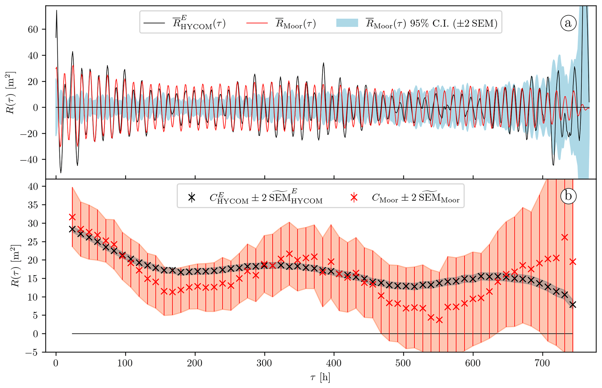
Figure 4 (a) Mean autocovariance computed from ${\mathit{\eta }}_{\mathrm{1000}}^{\mathrm{E}}$ (solid black curve, same as the solid red curve in Fig. 3a) and mean autocovariance computed from eleven 32 d segments of the mooring no. 2 time series (solid red curve) and 95 % confidence interval of ${\stackrel{\mathrm{‾}}{R}}_{\mathrm{Moor}}$ (light-blue shading). (b) Complex demodulates at the semidiurnal frequency of the autocovariance series shown in (a) and their 95 % C.I. The red and gray shadings highlight the 95 % C.I. for the mooring and Eulerian HYCOM data, respectively.

4 Results

4.1 The semidiurnal IT variance at 1000 dbar

We bin the global collection of HYCOM particles based on their median position using circular geographical patches of 200 km radius centered on a regular 2.5^∘ × 2.5^∘ grid. Here, we use only particles for which (i) the mean speed is lower than 0.1 m s⁻¹ (to avoid contamination by lee waves) and (ii) the variance of ${\mathit{\eta }}_{\mathrm{1000}}^{\mathrm{L}}$ is lower than 1×10⁴ m². The second criterion accounts for 41 discarded particles (out of 41 644) that we consider to be outliers, most of which are located in the Labrador Basin or in shallow water close to Antarctica. Including it instead would only marginally affect our results. We did not further investigate the cause of these extreme values.

As in Sect. 3.2 and 3.3, we compute an autocovariance series for each HYCOM particle, in the Lagrangian and Eulerian framework, separately. Then, we average these autocovariances over the corresponding patches to obtain local-mean autocovariance series ${\stackrel{\mathrm{‾}}{R}}_{\mathrm{HYCOM}}^{\mathrm{L}}$ and ${\stackrel{\mathrm{‾}}{R}}_{\mathrm{HYCOM}}^{\mathrm{E}}$. For each geographical patch, we get local estimates of the semidiurnal IT variance from the first 48 h complex demodulate of ${\stackrel{\mathrm{‾}}{R}}_{\mathrm{HYCOM}}^{\mathrm{L}}$ and ${\stackrel{\mathrm{‾}}{R}}_{\mathrm{HYCOM}}^{\mathrm{E}}$.

We start by checking how the Lagrangian sampling affects the semidiurnal IT variance. Figure 5 shows the first 48 h complex demodulate of ${\stackrel{\mathrm{‾}}{R}}_{\mathrm{HYCOM}}^{\mathrm{E}}$ plotted as a function of the first demodulate of ${\stackrel{\mathrm{‾}}{R}}_{\mathrm{HYCOM}}^{\mathrm{L}}$ for our collection of geographical patches. The agreement is close to perfect (with a Pearson r squared or coefficient of determination r²≈0.99 and 0.76 in the log–log and linear domain, respectively). Thus, the motion of the Lagrangian particles, and therefore of the Argo floats, has no significant impact on the measured variance of the IT.

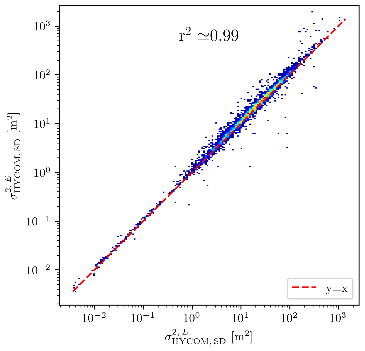
Figure 5 Semidiurnal IT variance estimated from the Eulerian HYCOM data as a function of the semidiurnal IT variance estimated from the Lagrangian HYCOM data for the unmasked bins in Fig. 6a. A warmer color indicates a larger density.

We can then map the semidiurnal IT variance (here taken as the first 48 h complex demodulate of ${\stackrel{\mathrm{‾}}{R}}_{\mathrm{HYCOM}}^{\mathrm{L}}$) and the associated $\stackrel{\mathrm{̃}}{\mathrm{SEM}}$ on a 2.5^∘ × 2.5^∘ grid (see Fig. 6a and b, respectively). In each figure we show only the bins which yield an IT variance larger than one $\stackrel{\mathrm{̃}}{\mathrm{SEM}}$. Note that the latter criterion is less binding than the one used for the global maps in Geoffroy and Nycander (2022) since the uncertainties are smaller here, by definition. Figure 6a can be directly compared with the global map of the semidiurnal IT variance computed from Argo data (see Fig. 6c and d, updated from Geoffroy and Nycander, 2022). As documented in Buijsman et al. (2020), HYCOM is known to be subject to a thermobaric instability (TBI) in the North Pacific (dashed black rectangle in Fig. 6a). Since only a few patches of Argo data are available at the edge of this TBI area, we do not exclude it from the subsequent analysis.

The main patterns visible in Fig. 6a and c broadly agree, with energy radiating away from low-mode IT generation hotspots, namely near Madagascar, Hawaii, French Polynesia, and the western South Pacific. In Fig. 7a we show the Argo-derived semidiurnal IT variance plotted as a function of the corresponding one from HYCOM. The two datasets are well correlated (r²=0.52 and 0.38 in the log–log and linear domain, respectively), but the semidiurnal IT variance is systematically smaller in HYCOM than in the Argo data.

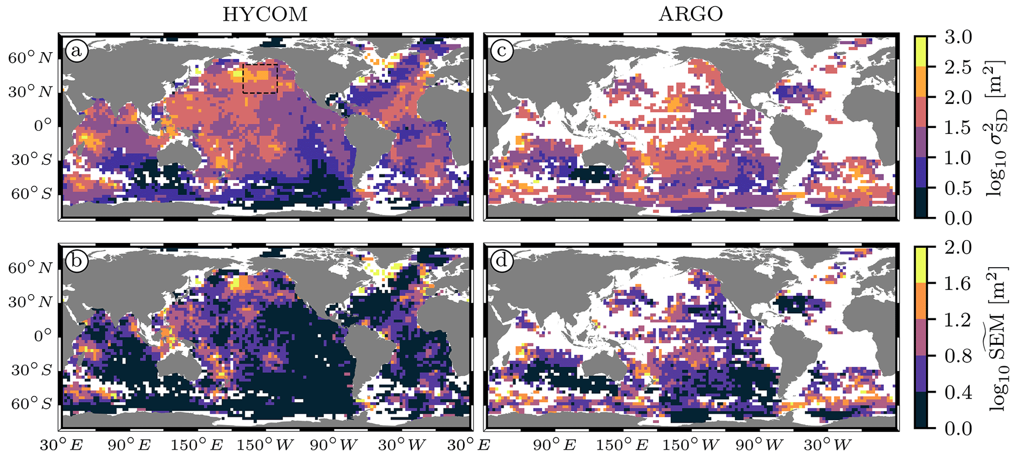
Figure 6 (a) Atlas of the semidiurnal IT variance computed as the first 48 h complex demodulate of the local-mean autocovariance series at 1000 dbar (${\stackrel{\mathrm{‾}}{R}}_{\mathrm{HYCOM}}^{\mathrm{L}}$) and (b) corresponding $\stackrel{\mathrm{̃}}{\mathrm{SEM}}$. (c, d) Same as (a) and (b), respectively, but computed from the Argo data (${\stackrel{\mathrm{‾}}{R}}_{\mathrm{Argo}}$). Panels (c) and (d) are updated from Geoffroy and Nycander (2022). The area where the simulation is affected by the TBI is shown by the dashed black rectangle in (a).

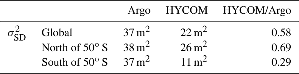
We investigate this bias by looking at the geographical distribution of the HYCOM-to-Argo semidiurnal IT variance ratio. For presentation purposes, instead of the latter ratio we plot the proxy ${\mathit{\sigma }}_{\mathrm{HYCOM}}^{\mathrm{2}}/({\mathit{\sigma }}_{\mathrm{HYCOM}}^{\mathrm{2}}+{\mathit{\sigma }}_{\mathrm{Argo}}^{\mathrm{2}})$ in Fig. 7b. This statistic is robust to outliers and maps a pair of variances to the closed range [0, 1]. The ratio is relatively homogeneous globally (in the range [0.25, 1.5], corresponding to [0.2, 0.6] for our proxy), except over the Southern Ocean, where the Argo-inferred IT variance is significantly larger. Furthermore, we show the zonal mean of the Argo- and HYCOM-derived semidiurnal IT variance as a function of latitude in Fig. 7c. The zonal-mean variance from Argo is generally larger, except around 40^∘ N, where the HYCOM-inferred zonal-mean variance peaks at 1.6 times the Argo one. Discarding the data in the TBI area has virtually no effect on this peak (not shown). More noteworthy than this localized feature, the ratio of the HYCOM to Argo zonal-mean variances decreases approaching the poles (poleward of ±50^∘ latitude, not shown). In contrast, equatorward of ±50^∘, this ratio remains fairly constant, oscillating around a mean value of 0.73 with a standard deviation of 0.26. The global mean and standard deviation of the ratio are 0.61 and 0.33, respectively.

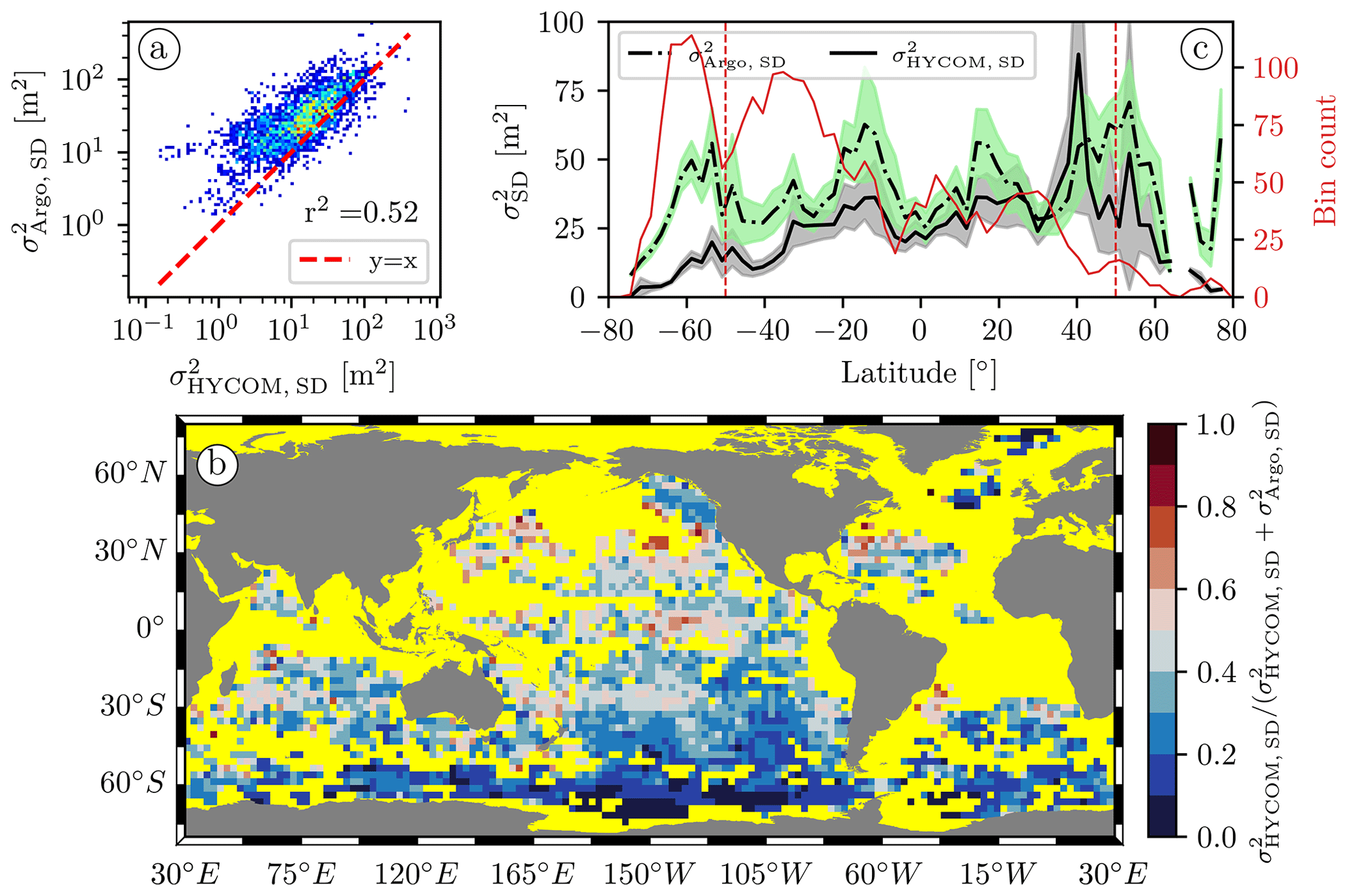
Figure 7 (a) Argo-derived semidiurnal IT variance as a function of the corresponding one from HYCOM for the collection of geographical bins shown in (b). A warmer color indicates a larger density. (b) Atlas of ${\mathit{\sigma }}_{\mathrm{HYCOM},\mathrm{SD}}^{\mathrm{2}}/({\mathit{\sigma }}_{\mathrm{HYCOM},\mathrm{SD}}^{\mathrm{2}}+{\mathit{\sigma }}_{\mathrm{Argo},\mathrm{SD}}^{\mathrm{2}})$, a proxy for the HYCOM-to-Argo semidiurnal IT variance ratio at 1000 dbar. The value of this proxy is close to 0 where ${\mathit{\sigma }}_{\mathrm{HYCOM},\mathrm{SD}}^{\mathrm{2}}\ll {\mathit{\sigma }}_{\mathrm{Argo},\mathrm{SD}}^{\mathrm{2}}$, 0.5 where ${\mathit{\sigma }}_{\mathrm{HYCOM},\mathrm{SD}}^{\mathrm{2}}\sim {\mathit{\sigma }}_{\mathrm{Argo},\mathrm{SD}}^{\mathrm{2}}$, and 1 where ${\mathit{\sigma }}_{\mathrm{HYCOM},\mathrm{SD}}^{\mathrm{2}}\gg {\mathit{\sigma }}_{\mathrm{Argo},\mathrm{SD}}^{\mathrm{2}}$. The ocean mask is colored in yellow for readability. (c) Zonal mean of the semidiurnal IT variance from Argo (dash-dotted black curve) and HYCOM (solid black curve) as a function of latitude and their respective 95 % C.I. (light-green and gray shading, respectively). The red curve represents the number of geographical bins used to compute the zonal mean at a given latitude (red axis on the right). The vertical dashed red lines are placed at 50^∘ S and 50^∘ N.

The representativity of the zonal-mean variances is smaller north of 40^∘ N because of the scarcity of available data (solid red curve in Fig. 7c). We therefore focus on the pronounced discrepancy affecting the Southern Ocean. We gather the data available over the unmasked bins in Fig. 7b into two groups, north and south of 50^∘ S. For each group and the global collection of bins, we compute a mean autocovariance by averaging the corresponding Argo and HYCOM local-mean autocovariance series (see Fig. 8). In Table 1, we summarize the semidiurnal IT variance values computed as the first 48 h demodulate of the mean autocovariance for each group. A significant fraction of the divergence visible in the global-mean autocovariance at short time lags (see Fig. 8a and b) can be explained by the larger discrepancy south of 50^∘ S (see Fig. 8e and f). In this region, the Argo-derived semidiurnal IT variance is close to 3.5 times larger than the simulated one. The agreement is better north of 50^∘ S, where the corresponding factor is 1.5 (see Fig. 8c and d). In a separate section we discuss possible explanations for both the lower semidiurnal IT variance in HYCOM globally and the even lower simulated IT variance in the Southern Ocean.

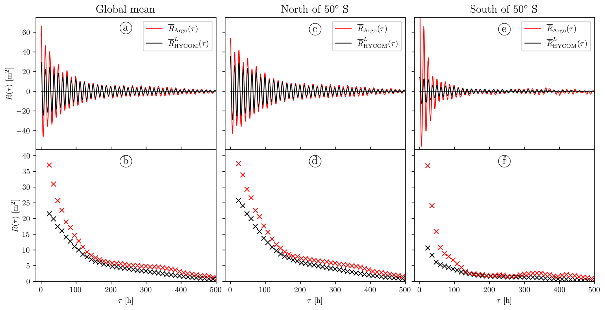
Figure 8 (a) Global-mean autocovariance at 1000 dbar computed from Argo data (solid red curve) and Lagrangian HYCOM particles (solid black curve) and (b) corresponding complex demodulates at the semidiurnal frequency. The uncertainties are vanishingly small (not shown). (c, d) Same as (a) and (b), respectively, but using only data north of 50^∘ S. (e, f) Same as (a) and (b), respectively, but using only data south of 50^∘ S. The Argo variance lies above the figure scale, here ${\stackrel{\mathrm{‾}}{R}}_{\mathrm{Argo}}\approx \mathrm{173}$ m². In this figure, we truncated τ at 500 h since past this limit the autocovariance series are close to 0.

Table 1 Semidiurnal IT variance from the autocovariance series plotted in Fig. 8.

4.2 The decorrelation of the semidiurnal IT at 1000 dbar

In contrast to Argo floats, the Eulerian sampling of moorings allows us to directly monitor the decorrelation of the IT. In a procedure similar to that in Sect. 4.1, we bin the global collection of HYCOM particles based on their median position, but this time using geographical patches (of 200 km radius) centered on the available moorings. We compute a sample autocovariance in the Eulerian framework for each particle and average them within the corresponding patches to obtain local-mean autocovariance series ${\stackrel{\mathrm{‾}}{R}}_{\mathrm{HYCOM}}^{\mathrm{E}}$. The mooring time series in a given patch is split into successive 32 d segments. We then compute a sample autocovariance for each segment and average them to obtain a mean autocovariance ${\stackrel{\mathrm{‾}}{R}}_{\mathrm{Moor}}$. Again, we use only particles for which (i) the mean speed is lower than 0.1 m s⁻¹ (to avoid contamination by lee waves) and (ii) the variance of ${\mathit{\eta }}_{\mathrm{1000}}^{\mathrm{L}}$ is lower than 1×10⁴ m² (outliers). After some additional quality controls, mainly discarding bins where either the mooring or HYCOM complex demodulates fall under one $\stackrel{\mathrm{̃}}{\mathrm{SEM}}$ within 15 d of time lag, we are left with 172 moored instruments and the corresponding patches of simulated data.

For all the datasets used in this study, we found the probability distribution of the global collection of local-mean autocovariance at any given time lag to be skewed (not shown). This is not an issue when computing average statistics from the Argo or the corresponding simulated data, since the number of samples (i.e., the number of geographical bins) is very large, and the sample mean is therefore expected to be normally distributed, by virtue of the central limit theorem. In contrast, geographical bins where mooring data are available are fewer. Thus, the influence of the tail of the distribution on the sample mean is larger when analyzing the relatively small collection of bins where mooring data are available than when considering the global collections of Argo and HYCOM data. This precludes the use of statistics that assume a normal distribution when describing regional or even global averages of the autocovariances computed from moorings. To limit the effects of skewness, we discard bins for which either the mooring or the simulated first 48 h demodulate is above the 95th percentile of its observed distribution (here $P_{\mathrm{Moor}}^{\mathrm{95}}\approx \mathrm{575}$ m² and $P_{\mathrm{HYCOM}}^{\mathrm{95}}\approx \mathrm{330}$ m², respectively). The latter criterion accounts for 12 additional discarded bins, all located in moderate- to strong-mesoscale-activity areas. Even after discarding these extreme samples, the data remain highly skewed.

The moorings may not offer as much spatial coverage as the Argo floats do, but they still provide an opportunity to validate the geographical variability in the semidiurnal IT variance in HYCOM. As in Sect. 4.1, we can get local estimates of the semidiurnal IT variance from ${\stackrel{\mathrm{‾}}{R}}_{\mathrm{HYCOM}}^{\mathrm{E}}$ and ${\stackrel{\mathrm{‾}}{R}}_{\mathrm{Moor}}$ in each geographical patch centered on a mooring. Figure 9a shows the scatterplot of the first 48 h complex demodulate of ${\stackrel{\mathrm{‾}}{R}}_{\mathrm{HYCOM}}^{\mathrm{E}}$ as a function of the first demodulate of ${\stackrel{\mathrm{‾}}{R}}_{\mathrm{Moor}}$ for our collection of geographical bins. As with the Lagrangian data (see Fig. 7a), the correlation is good (r²=0.51 and 0.40 in the log–log and linear domain, respectively), but the semidiurnal IT variance is systematically smaller in HYCOM than in the mooring data. In Fig. 9b and c we show the geographical location of the patches along with a proxy for the HYCOM-to-mooring semidiurnal IT variance ratio and the histogram of this proxy, respectively. The latter histogram shows that the distribution of the proxy is centered around 0.37, corresponding to a ratio of 0.6, approximately.

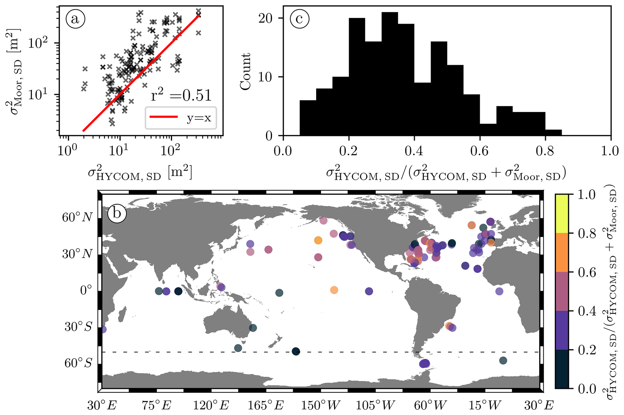
Figure 9 (a) Semidiurnal IT variance derived from mooring data as a function of the semidiurnal IT variance computed from the Eulerian HYCOM data. (b) Map of the 160 geographical bins presented in (a) along with the proxy ${\mathit{\sigma }}_{\mathrm{HYCOM},\mathrm{SD}}^{\mathrm{2}}/({\mathit{\sigma }}_{\mathrm{HYCOM},\mathrm{SD}}^{\mathrm{2}}+{\mathit{\sigma }}_{\mathrm{Moor},\mathrm{SD}}^{\mathrm{2}})$ for the ratio of the semidiurnal IT variance computed from the Eulerian HYCOM and mooring data and (c) the histogram of this proxy. An equivalent proxy was used in Fig. 7b. The dashed black line in (b) indicates 50^∘ S.

To measure the strength of the decorrelation affecting the Eulerian mean autocovariances, we define the semidiurnal coherent variance fraction (SCVF₁₅) as the ratio between the 48 h demodulate at τ≈15 d (i.e., one spring–neap period) and the first demodulate. As it is calculated from the demodulate at relatively long time lags, the SCVF₁₅ is meaningful only when estimated from a large enough sample size (i.e., with minimal uncertainty). Therefore, we start by considering all the data available over our global collection of geographical bins.

Figure 10a displays the global-mean autocovariances calculated from the mooring (${\stackrel{\mathrm{‾}}{R}}_{\mathrm{Moor}}$, solid red curve) and HYCOM data (${\stackrel{\mathrm{‾}}{R}}_{\mathrm{HYCOM}}$, solid black curve), as the average of the local-mean autocovariance series over the bins presented in Fig. 9b. In Fig. 10b we show different statistics of the observed distribution of the demodulates of the local-mean autocovariances in the form of boxplots as a function of time lag. Figure 10b suggests that the mooring records exhibit both a larger semidiurnal IT variance and a stronger decorrelation on average globally: the mean of the first demodulates and the mean SCVF₁₅ are 76 m² and 0.47 as well as and 41 m² and 0.57 for the moorings and HYCOM data, respectively. Using median values instead leads to the same conclusions (not shown).

We investigate a potential latitudinal dependence by plotting the mean autocovariance series computed separately from the geographical bins lying north (149 instruments) and south (11 instruments) of 50^∘ S (see Figs. 10c and d, and 10e and f, respectively). The mean semidiurnal IT variance and the mean SCVF₁₅ for each group are shown in Table 2. Again, the divergence between the two datasets appears enhanced south of 50^∘ S. Moreover, the SCVF₁₅ is larger in the Southern Ocean than elsewhere for HYCOM but smaller for the moorings. This indicates a weaker, or slower, decorrelation of the IT in HYCOM in the Southern Ocean than in the global ocean.

The slower decorrelation of the IT in the simulation can be explained by some decorrelating processes, such as eddies or submesoscale variability, being weaker in HYCOM than in the real ocean. It could also be explained by the time variability in certain decorrelating processes. Our numerical simulation only spans 20 May to 20 June 2019. Therefore, it is potentially missing processes that would specifically occur or intensify at another time of the year (or in a different year). On the other hand, the mooring data span several decades. Thus, our single month of data from HYCOM may not be representative of the broader temporal sampling of the mooring data.

The spatial distribution of the moorings is sparse and tends to be denser in particular areas (e.g., the Gulf Stream region). This is all the more true south of 50^∘ S, where much fewer moorings are available than in the northern region and where they are mostly located in the Drake Passage. For both these reasons, the mean autocovariances computed from moorings north and especially south of 50^∘ S cannot be considered truly representative of the IT in these vast regions. Nonetheless, they remain representative of the collection of geographical bins used to construct them.

Table 2 Summarizing numerics of the autocovariance series plotted in Fig. 10.

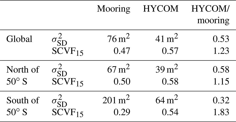
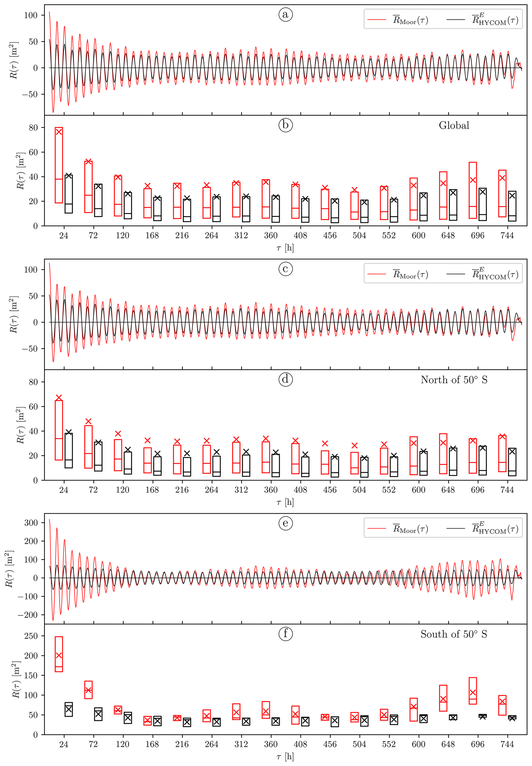
Figure 10 (a) Global-mean autocovariance computed as the average of the local-mean autocovariance series from the HYCOM particles over the geographical bins presented in Fig. 9b (solid black curve) and global-mean autocovariance from the moored instruments computed in the same way (solid red curve). (b) Boxplots of the observed distribution of the complex demodulates at the semidiurnal frequency of the local-mean autocovariances for the collection of geographical bins presented in Fig. 9b as a function of time lag. Each boxplot consists of a rectangle extending from the first to the third quartile of the data, with a line at the median and a cross at the mean. For a given time lag, the red and black boxplots, offset on either side of the time lag value, represent the distribution of the demodulates computed over the 48 h window centered on that time lag value from moorings and HYCOM, respectively. (c, d) Same as (a) and (b), respectively, but using only the 149 geographical bins north of 50^∘ S. (e, f) Same as (a) and (b), respectively, but using only the 11 geographical bins south of 50^∘ S.

4.3 Apparent decorrelation

In Sect. 4.1 we demonstrated that the motion of the floats has no significant impact on the measured total variance of the IT. However, the Doppler effect and spatial decorrelation induced by the Lagrangian sampling of the floats both act as decorrelating processes causing the autocovariance to decay with increasing time lag (Geoffroy and Nycander, 2022). Following Caspar-Cohen et al. (2022), we call this mechanism apparent decorrelation, as it is unrelated to the decorrelation of the IT. Geoffroy and Nycander (2022) estimated the apparent decorrelation timescale to be longer than that of the autocovariance function observed by Argo floats, on average globally. Thus, they concluded that the decay of the global-mean autocovariance observed by Argo floats is primarily due to the decorrelation of the IT.

The HYCOM data allow this to be studied by directly comparing the global-mean autocovariance computed in the Lagrangian and Eulerian frameworks (see Fig. 11a and b). As expected, the Lagrangian (${\stackrel{\mathrm{‾}}{R}}_{\mathrm{HYCOM}}^{\mathrm{L}}$, solid black curve in Fig. 11a) and Eulerian (${\stackrel{\mathrm{‾}}{R}}_{\mathrm{HYCOM}}^{\mathrm{E}}$, solid red curve) global-mean autocovariances are virtually identical until τ≈50 h. Past this limit, the more rapid decay of ${\stackrel{\mathrm{‾}}{R}}_{\mathrm{HYCOM}}^{\mathrm{L}}$ can only be caused by the apparent decorrelation, while ${\stackrel{\mathrm{‾}}{R}}_{\mathrm{HYCOM}}^{\mathrm{E}}$ continues to solely reflect the decorrelation of the IT. Our aim in the present section is to find estimates for the characteristic timescales of the apparent decorrelation and decorrelation of the IT in HYCOM and compare them with observations.

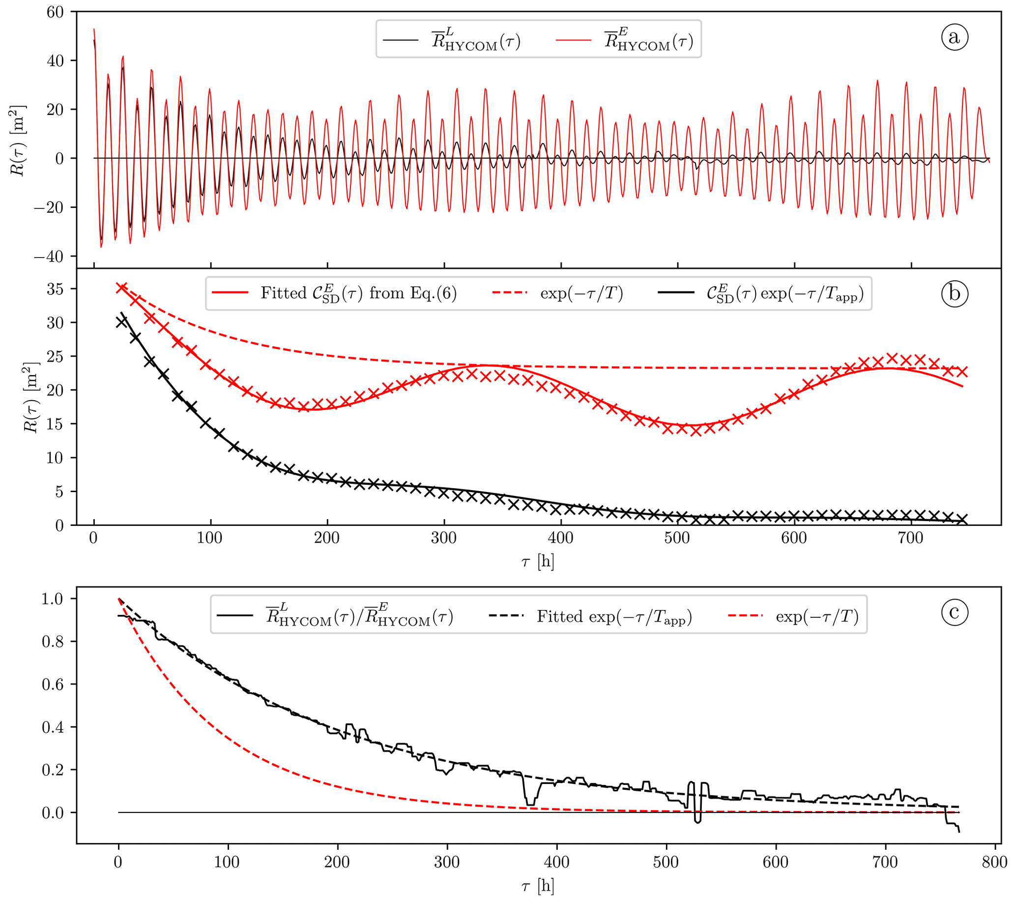
Figure 11 (a) Global-mean autocovariance at 1000 dbar computed from the global collection of HYCOM-derived η^L (solid black curve) and η^E (solid red curve) time series and (b) corresponding complex demodulates at the semidiurnal frequency. The uncertainties are vanishingly small (not shown). The solid and dashed red curves represent the result of fitting the model Eq. (5) to the Eulerian demodulates and the underlying exponential decay due to the decorrelation of the IT, respectively. The solid black curve corresponds to the model Eq. (6) with the different parameters set as described in the text. (c) Median filtered ratio of ${\stackrel{\mathrm{‾}}{R}}_{\mathrm{HYCOM}}^{\mathrm{L}}$ to ${\stackrel{\mathrm{‾}}{R}}_{\mathrm{HYCOM}}^{\mathrm{E}}$ (solid black curve) and fitted decaying exponential with the apparent decorrelation timescale (dashed black curve). For reference, we overlay a decaying exponential with the IT decorrelation timescale obtained by fitting the model Eq. (5) to the Eulerian demodulates (dashed red curve).

Taking inspiration from Geoffroy and Nycander (2022) and Caspar-Cohen et al. (2022), we try a simple model for the complex demodulate at the semidiurnal frequency of the Eulerian autocovariance computed over a time lag window centered on τ:

$$\begin{array}{}\text{(5)}& \begin{array}{rl}{\mathcal{C}}_{\mathrm{SD}}^{\mathrm{E}}\left(\mathit{\tau }\right)& ={\mathit{\sigma }}_{\mathrm{SD}}^{\mathrm{2}}(\mathit{\alpha }+(\mathrm{1}-\mathit{\alpha }\left)\exp \right(-\mathit{\tau }/T\left)\right)\\ & +{\mathit{\sigma }}_{\mathrm{AM}}^{\mathrm{2}}\left(\cos \right({\mathit{\omega }}_{\mathrm{AM}}\mathit{\tau })-\mathrm{1}).\end{array}\end{array}$$

Here, ${\mathit{\sigma }}_{\mathrm{SD}}^{\mathrm{2}}$ is the total semidiurnal internal tide variance; α is the stationary fraction; T is the IT decorrelation timescale; and ${\mathit{\sigma }}_{\mathrm{AM}}^{\mathrm{2}}$ and ω_AM are the variance and angular frequency of an amplitude-modulating sinusoid, respectively. A heuristic model for the demodulate of the corresponding Lagrangian autocovariance is then

$$\begin{array}{}\text{(6)}& {\mathcal{C}}_{\mathrm{SD}}^{\mathrm{L}}\left(\mathit{\tau }\right)={\mathcal{C}}_{\mathrm{SD}}^{\mathrm{E}}\left(\mathit{\tau }\right)\exp (-\mathit{\tau }/T_{\mathrm{app}}),\end{array}$$

where T_app is the apparent decorrelation timescale.

A constrained least squares fit of the model Eq. (5) to the complex demodulate series computed from ${\stackrel{\mathrm{‾}}{R}}_{\mathrm{HYCOM}}^{\mathrm{E}}$ (red crosses in Fig. 11b) yields T=94 h. The fitted model and the exponential decay due to the IT decorrelation (i.e., only the term proportional to ${\mathit{\sigma }}_{\mathrm{SD}}^{\mathrm{2}}$) are represented in Fig. 11b as the solid and dashed red curves, respectively. On average globally, 95 % of the decorrelation of the nonstationary IT in HYCOM is therefore achieved within 3T≈300 h (for $\exp (-\mathrm{3})\approx \mathrm{0.05}$), i.e., well under the 32 d of data.

By dividing ${\stackrel{\mathrm{‾}}{R}}_{\mathrm{HYCOM}}^{\mathrm{L}}$ by ${\stackrel{\mathrm{‾}}{R}}_{\mathrm{HYCOM}}^{\mathrm{E}}$, we can isolate the effects of the apparent decorrelation on ${\stackrel{\mathrm{‾}}{R}}_{\mathrm{HYCOM}}^{\mathrm{L}}$. In Fig. 11c we plot this ratio after applying a median filter with a window of 18 h (solid black curve). A least squares fit of a simple decaying exponential to the obtained curve yields an apparent decorrelation timescale T_app=209 h (dashed black curve). For verification, we compute the Lagrangian ${\mathcal{C}}_{\mathrm{SD}}^{\mathrm{L}}$ from Eq. (6) by multiplying the fitted model of ${\mathcal{C}}_{\mathrm{SD}}^{\mathrm{E}}$ (solid red curve in Fig. 11b) by the fitted exponential decay due to the apparent decorrelation (dashed black curve in Fig. 11c). The result (solid black curve in Fig. 11b) closely follows the demodulated Lagrangian autocovariance (black crosses in Fig. 11b). The different parameters obtained from the Eulerian and Lagrangian simulated data are summarized in Table 3. Note that the fitted amplitude-modulating sinusoid is close to the spring–neap cycle, here ${\mathit{\omega }}_{\mathrm{AM}}=|{\mathit{\omega }}_{{\mathrm{M}}_{\mathrm{2}}}-{\mathit{\omega }}_{{\mathrm{S}}_{\mathrm{2}}}|\approx \mathrm{0.0177}$ h⁻¹.

Table 3 Summary of the parameters estimated from the simulated Eulerian and Lagrangian data. These values are used to compute ${\mathcal{C}}_{\mathrm{SD}}^{\mathrm{L}}$ from the model Eq. (6) (solid black curve in Fig. 10b).

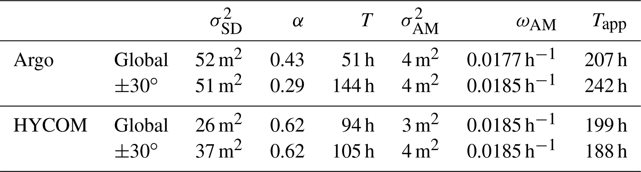
We can compare the global-mean values of T and T_app obtained from the simulation with the Argo observations. The geographical coverage of the Argo data is less than that of HYCOM (roughly 55 % in area). Hence, instead of the global collections of floats and Lagrangian particles, we now consider the intersection of the two datasets taken as the unmasked bins shown in Fig. 7b and the corresponding local-mean autocovariances. These local-mean autocovariances are averaged further to obtain a global-mean autocovariance for each dataset that is representative of a common area. We then fit the model Eqs. (6) and (5) to the demodulates of the Argo global-mean autocovariance (see Fig. 12, updated from Geoffroy and Nycander, 2022). The parameters fitted to the Argo observations, as well as the parameters obtained by repeating the above procedure for the corresponding simulated data, are gathered in Table 4. The values of T_app and T computed here, from Argo data only, are similar to those reported by Geoffroy and Nycander (2022), where the authors estimated them from a comparable collection of Argo floats and HRET (in particular, the stationary limit was determined from HRET instead of by fitting). The fitted stationary fraction α, however, is about 3 times larger than previously reported. This could be explained by a low-biased stationary variance (obtained by projecting HRET at 1000 dbar) in Geoffroy and Nycander (2022). As from the simulated data, fitting our model to the Argo global-mean demodulates yield a T shorter than T_app. While the Argo T_app is almost identical to the HYCOM value, T is about twice as small.

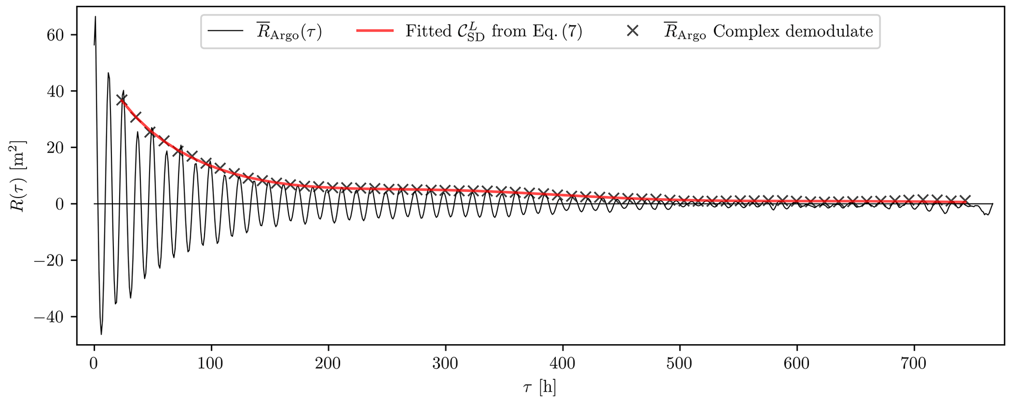
Figure 12 Global-mean autocovariance at 1000 dbar computed from the Argo data over the unmasked bins in Fig. 7b (solid black curve) and corresponding complex demodulates at the semidiurnal frequency (black crosses). The uncertainties are vanishingly small (not shown). The solid red curve represents the result of fitting the model Eqs. (6) and (5) to the demodulates.

Similarly to Geoffroy and Nycander (2022), we conclude that the decorrelation of the IT is more rapid than the apparent decorrelation on average globally. Yet, according to the simulated data, it is only more rapid by a factor of 2, while this factor is 4 according to the Argo data. Hence, some decorrelating processes appear to be weaker in the simulation than in the real ocean. As explained in Sect. 4.2, the slower decorrelation of the IT in HYCOM could also be explained by certain decorrelating processes being weaker than usual in the 20 May–20 June 2019 period of outputs used here. Nevertheless, the decorrelation of the IT typically is at least as important as the apparent decorrelation over the first few days of time lag. This result might not hold true everywhere, since the geographical variability in T and α is expected to be large.

Lastly, Zaron (2022) provides a valuable comparison point for the results above. Along the same lines as in this section, he uses the spatially averaged frequency spectrum of sea level observations from satellite altimetry to measure properties of both the baroclinic tidal peak and continuum (i.e., the coherent and incoherent IT variability, respectively). For the semidiurnal band, in the latitude range from 30^∘ S to 30^∘ N, the author found that about 62 % of the IT variance eventually becomes decorrelated within 34 d. Assuming an exponential decay as in the model Eq. (5), this would represent a stationary fraction α≈0.38 and a decorrelation timescale T≈163 h (for 99 % of the nonstationary IT to decorrelate in 5T). Repeating the fitting procedure above for data limited to the ±30^∘ latitude range, we recover values in reasonable agreement from the Argo observations: α≈0.29 and T≈144 h (see Table 4). The HYCOM-fitted α≈0.64 and T≈105 h agree less well with the results of Zaron (2022) but still are in the same ballpark. In this latitude range, the bins used for the fitting represent roughly 45 % of the oceanic area.

Table 4 Parameters from the fitting of the model Eq. (6) to the demodulates of (i) the global-mean autocovariance computed from the Argo data over the unmasked bins in Fig. 7b (see Fig. 12) and (ii) the mean autocovariance computed from the same bins but limited to the latitude range from 30^∘ S to 30^∘ N. These parameters are also estimated from the simulated Eulerian and Lagrangian data in the same locations.

4.4 Potential sources of bias

Why is the IT variance lower and IT decorrelation weaker in HYCOM than in the observations, particularly in the Southern Ocean? At the time of writing we cannot think of a particular reason for either the Argo- or the mooring-derived IT variance to be biased high globally. In particular, the correction accounting for the non-tidal variability we systematically subtract from the sample autocovariance precludes any contamination of the first demodulate by the background noise (see Appendix C).

We also investigated whether the bias in the Southern Ocean could be related to the contamination of the first 48 h demodulate at ω_SD by near-inertial waves as we approach the M₂ critical latitude (where $f={\mathit{\omega }}_{{\mathrm{M}}_{\mathrm{2}}}$, at about 74^∘ S). To check this, we can map the semidiurnal IT variance from the Argo data anew (as shown in Fig. 6c), this time fitting an additional cos (fτ), where f is the local Coriolis frequency, to the local-mean autocovariances. The result of the fit becomes unstable at 74^∘ S, but the zonal mean of the demodulates at f does reach a maximum around 60^∘ S, while the zonal mean of the demodulates at ω_SD remains unaffected (not shown). We conclude that the first 48 h demodulate at the semidiurnal frequency is not affected by near-inertial waves at any latitude.

As for the model, the horizontal grid spacing limits the number of vertical modes correctly resolved to the first five modes, equatorward of ±50^∘ latitude and for seafloor depths deeper than 1250 m (Buijsman et al., 2020). Approaching the poles, the number of model layers below the mixed layer, and hence the vertical resolution, decreases. This further limits the number of resolved modes in HYCOM south of 50^∘ S: roughly, modes 3 and 2 are only partially resolved poleward of 60 and 65^∘ S, respectively. Although the bulk of the IT variance at 1000 dbar is likely related to mode-1 waves on average globally (Geoffroy and Nycander, 2022), the contribution from higher modes can become significant locally. In principle, Argo floats, moorings, and HYCOM data include the effect of higher modes, but these are less well resolved in HYCOM, particularly in the Southern Ocean. Together with the assumption that higher-mode ITs are less coherent (Egbert and Ray, 2017), this may explain the lower IT variance and weaker IT decorrelation in HYCOM than in the observations, both on average globally and more specifically in the Southern Ocean. It is also in line with the larger mean SCVF₁₅ computed from HYCOM data in the Southern Ocean compared with the rest of the globe (indicating a weaker decorrelation there), whereas for moorings the SCVF₁₅ is smaller in this region (see Table 2).

The mode-m vertical structure of the isopycnal displacement Φ_m(z) is obtained by solving the Sturm–Liouville problem

$$\begin{array}{}\text{(7)}& {\displaystyle \frac{{\mathrm{d}}^{\mathrm{2}}{\mathrm{\Phi }}_m\left(z\right)}{\mathrm{d}{z}^{\mathrm{2}}}}+{\displaystyle \frac{N^{\mathrm{2}}\left(z\right)}{c_m^{\mathrm{2}}}}{\mathrm{\Phi }}_m\left(z\right)=\mathrm{0},\end{array}$$

with the boundary conditions ${\mathrm{\Phi }}_m\left(\mathrm{0}\right)={\mathrm{\Phi }}_m(-H)=\mathrm{0}$, where H is the ocean depth, N(z) is the buoyancy frequency profile, and $-\mathrm{1}/c_m^{\mathrm{2}}$ is the eigenvalue corresponding to the eigenfunction Φ_m(z) for mode-m (Gill, 1982). The modal partitioning of the IT energy at a given location is mainly determined by the conversion rate (both local and remote) and lifetime of each mode (de Lavergne et al., 2019). Additionally, depending on the local stratification and ocean depth, the parking depth at 1000 dbar can be more or less close to the anti-node (point of maximal displacement) and node (point of no displacement) of the different vertical modes. Therefore, the normalized contribution of mode-m relative to mode-1 waves to the variance recorded at this depth is weighted by a coefficient γ_m1. In Appendix B of Geoffroy and Nycander (2022), the authors derived an expression for this coefficient:

$$\begin{array}{}\text{(8)}& {\mathit{\gamma }}_{m\mathrm{1}}\left(z\right)={\displaystyle \frac{{\mathrm{\Phi }}_m^{\mathrm{2}}\left(z\right){\int }_{-H}^{\mathrm{0}}{N}^{\mathrm{2}}{\mathrm{\Phi }}_{\mathrm{1}}^{\mathrm{2}}\mathrm{d}z}{{\mathrm{\Phi }}_{\mathrm{1}}^{\mathrm{2}}\left(z\right){\int }_{-H}^{\mathrm{0}}{N}^{\mathrm{2}}{\mathrm{\Phi }}_m^{\mathrm{2}}\mathrm{d}z}}.\end{array}$$

In Fig. 13a and b we plot the global maps of γ₂₁ and γ₃₁ at 1000 dbar, respectively, computed from Eq. (8) after solving the eigenvalue problem Eq. (7) for the $\mathrm{1}/\mathrm{4}$^∘ WOA18 summer climatology. Here, we extrapolated the climatological data down to the reference bathymetry from the General Bathymetric Chart of the Oceans 2019 (GEBCO, 2019) wherever the bathymetry is deeper than the deepest valid climatological record. A visual comparison with Fig. 7b in the Southern Ocean suggests that low HYCOM-to-Argo IT variance ratios (darker-blue pixels in Fig. 7b) spatially coincide with large γ₃₁ mostly or, to some extent, γ₂₁ (especially in the Weddell Sea). South of 60^∘ S, either γ₃₁ or γ₂₁ is larger than unity; hence the contribution from mode-3 or mode-2 waves to the IT variance recorded at 1000 dbar is magnified compared to the contribution from mode-1 waves. However, modes 2 and higher are not well resolved in HYCOM at these latitudes.

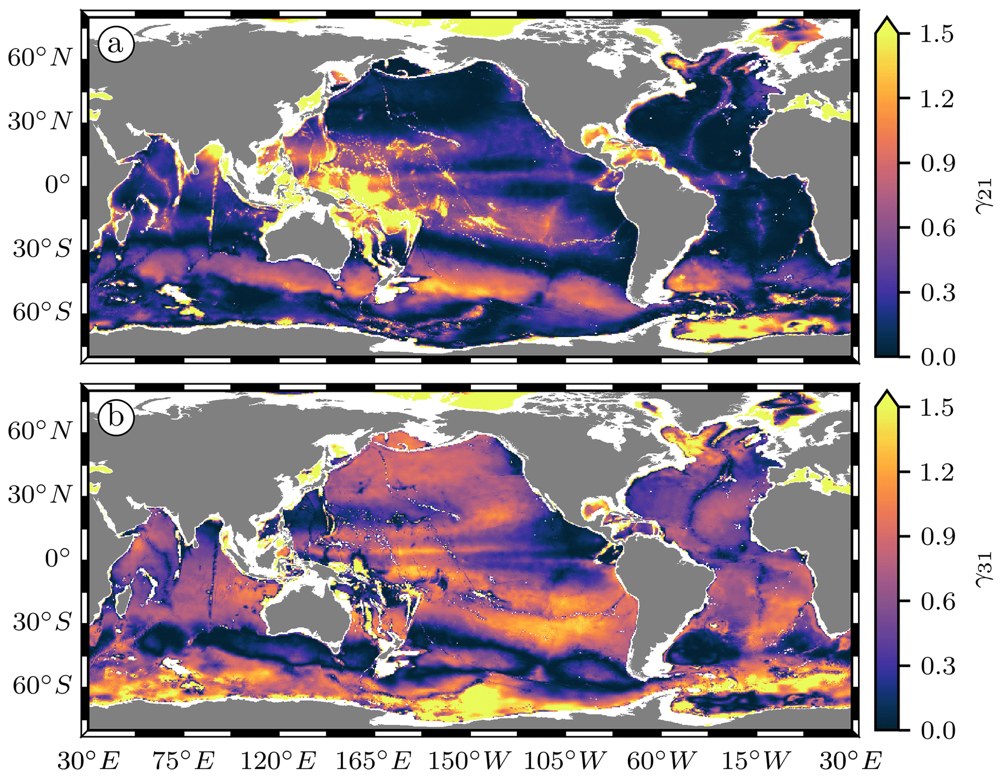
Figure 13 (a) Weight of the normalized contribution of mode-2 relative to mode-1 waves to the IT variance recorded at 1000 dbar, computed from the WOA18 stratification. (b) Same as (a) but for the relative contribution of mode-3 waves.

The magnification of the contributions from modes 2 and 3 to the variance at 1000 dbar in the Southern Ocean only affects how propagating ITs are perceived at the Argo parking depth. This has no connection with the generation and dissipation processes that set the underlying modal partitioning of the IT energy. Additional explanations might be found by examining whether the main parameters affecting the generation of ITs (namely the bottom topography, barotropic tidal forcing, and stratification) are less accurate in this region than in the rest of the globe.

The pattern of the enhanced discrepancies between Argo and HYCOM in the Southern Ocean (darker blue in Fig. 7) might be correlated with the distribution of bathymetric features. For instance, the large values around 45^∘ S, 105^∘ W, in the South Pacific are centered on the Chile Rise, a known IT generation area. To date, only about 19 % of the global ocean seafloor has been mapped using shipborne techniques. Therefore, global bathymetric products widely rely on depth prediction from satellite gravimetry (Smith and Sandwell, 1994). Small-scale features such as abyssal hills are not resolved by this technique.

In the recent SRTM15+ bathymetry (Tozer et al., 2019), gravity-predicted depths were estimated to have root mean square (RMS) uncertainties and maximum error of the order of ±150 and 1800 m, respectively (based on 50 cruises distributed globally). With about 22 % seafloor coverage by direct high-quality measurements, the International Bathymetric Chart of the Southern Ocean v2 (IBCSO; Dorschel et al., 2022) is the state-of-the-art bathymetric chart south of 50^∘ S. A cell-by-cell comparison between IBCSO v2 and SRTM15+ v2.2 showed marked disparities, in particular for water depths between −4000 and −1000 m with differences reaching up to 1700 m (Dorschel et al., 2022). Most of the bathymetric errors only affect the generation of high-mode ITs, which are bound to dissipate locally. Note that HYCOM may not resolve these high-mode ITs anyway, as discussed in the present section. Still, the less frequent errors of the order of thousands of meters are likely to affect the generation of low-mode ITs in the model.

Efforts have been made to improve the accuracy of the M₂ barotropic tides embedded in HYCOM. The simulation used in this study incorporates the framework presented in Ngodock et al. (2016) aiming at minimizing the tidal elevation RMS errors with respect to TPXO, a state of the art data-assimilative tide model (Egbert and Erofeeva, 2002). However, the tidal elevations in TPXO itself also have errors. Both Stammer et al. (2014) and Zaron and Elipot (2021) point at the imperfection of the modeled tidal elevations near Antarctica (using data from GRACE and CryoSat-2, respectively). On the other hand, it is not so much the sea surface height that matters here, but the tidal currents. Zaron and Elipot (2021) used surface drifter observations for evaluating TPXO-predicted tidal currents throughout much of the global oceans. Unfortunately, the spatial density of observations is too poor to evaluate the model performance around much of Antarctica.

Lastly, to assess the stratification in HYCOM, we compare the phase speed of a mode-1 gravity wave in the model with the phase speed determined from climatology. The phase speed of a mode-m gravity wave c_m is directly related to the eigenvalue $-\mathrm{1}/c_m^{\mathrm{2}}$ obtained by solving the Sturm–Liouville problem (Eq. 7). Having already solved Eq. (7) for the climatology, we now solve it for our simulated monthly mean 3D fields of temperature and salinity (subsampled to 1^∘). As for the climatology, the HYCOM data were extended down to the reference bathymetry from GEBCO 2019, wherever deeper, by appending the stored bottom value. We then linearly interpolated the climatological phase speed of a mode-1 gravity wave $c_{\mathrm{1}}^{\mathrm{WOA}}$ at $\mathrm{1}/\mathrm{4}$^∘ resolution onto the coarser 1^∘ HYCOM grid.

In Fig. 14a we plot the climatology-to-HYCOM phase speed ratio. Most of the visible differences fall in the range of expected interannual variability of less than 10 % (Chelton et al., 1998). However, in a few areas around Antarctica there are larger departures of the ratio from unity. Figure 14b shows the zonal mean of the mode-1 phase speed from Argo and HYCOM as a function of latitude. Equatorward of ±60^∘, the two curves agree almost perfectly, and they also visually agree with the results of Chelton et al. (1998) (not shown). Poleward of 60^∘ S and 60^∘ N, however, differences steadily grow. In the Southern Ocean, the zonal-mean-climatology-to-HYCOM phase speed ratio peaks at 1.7 (see Fig. 14c). Typically, weaker stratification (smaller phase speed) results in smaller energy conversion.

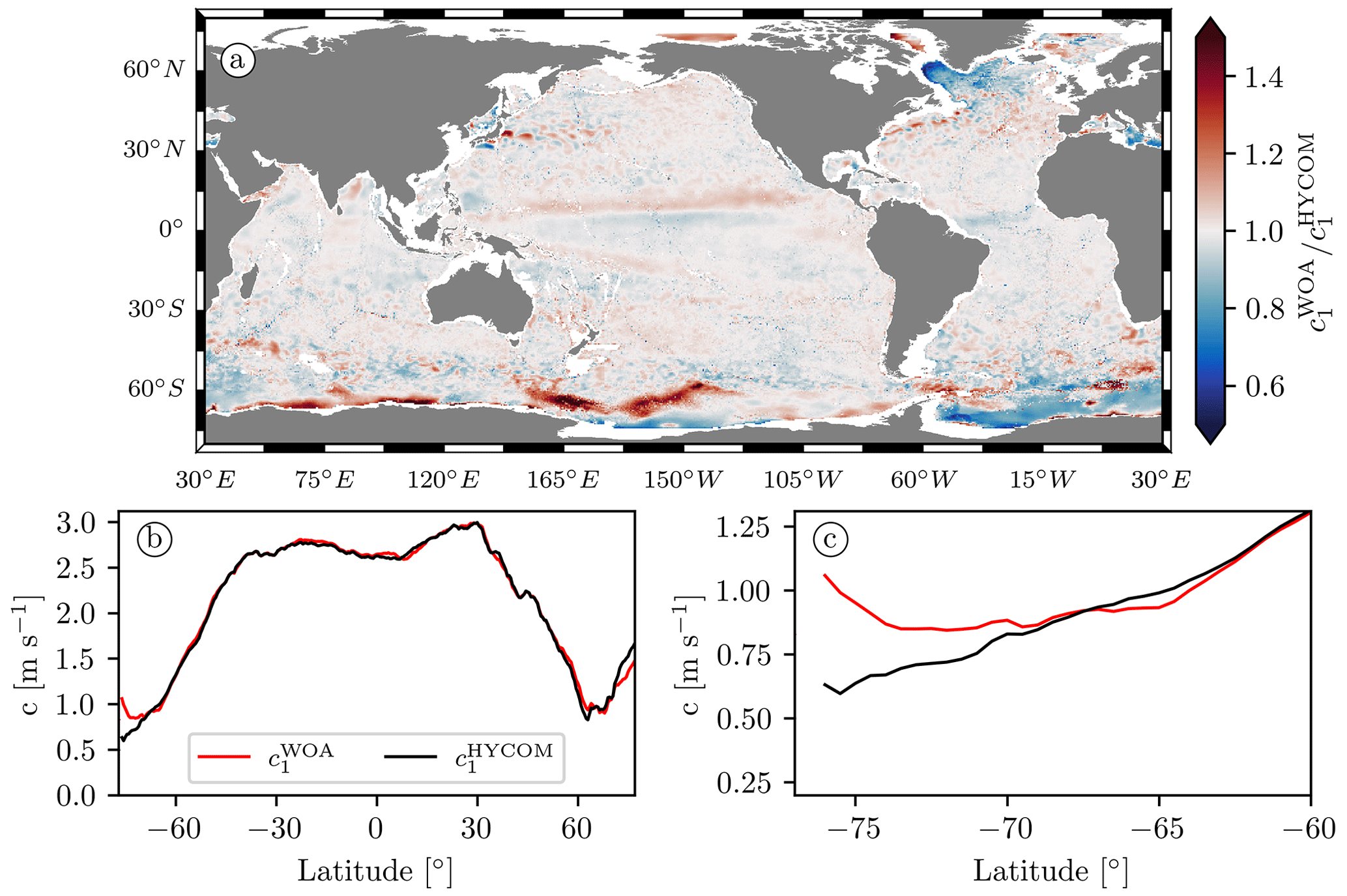
Figure 14 (a) Ratio of the phase speeds of a mode-1 gravity wave computed from the WOA18 and HYCOM stratification profiles. (b) Zonal mean of the phase speed of a mode-1 gravity wave from WOA18 (solid red curve) and HYCOM (solid black curve) as a function of latitude. (c) Same as (b) but zoomed in between 77 and 60^∘ S.

5 Conclusions

In this work we compare a 32 d segment of a global run of the HYCOM model, including realistic tidal and atmospheric forcing, with in situ observations of the semidiurnal IT around 1000 dbar. First, a Lagrangian sampling of the simulation was compared to park-phase data from Argo floats to validate the geographical variability in the semidiurnal IT variance in HYCOM (see Sect. 4.1). Then, the Eulerian simulation outputs were directly compared to geographically sparser mooring records, in terms of variance and decorrelation of the IT (see Sect. 4.2).

The main spatial patterns of the simulated IT variance at 1000 dbar broadly agree with Argo observations, with energy radiating away from low-mode IT generation hotspots (see Fig. 6). Nonetheless, on average globally, the HYCOM data exhibit a smaller semidiurnal IT variance than observed by Argo floats, by a factor 0.58 (see Table 1). This is in line with the results of Ansong et al. (2017) and Luecke et al. (2020), who found HYCOM values to be biased low by a similar factor when comparing the simulated M₂ IT energy flux and temperature variance to historical mooring observations.

While the difference between the model and Argo data appears reasonably homogeneous across most of the world ocean, it steadily increases towards the poles (see Fig. 7). Because of the scarcity of Argo floats available in the northernmost region, we focused on the Southern Ocean. On average, south of 50^∘ S, we found that the simulated semidiurnal IT variance is smaller than the variance observed by Argo by a factor of 0.29. North of 50^∘ S, this factor is 0.69 (see Table 1).

The mooring data support the above results for the semidiurnal IT variance. Additionally, we found that the decorrelation affecting the semidiurnal IT in HYCOM over a 32 d window is weaker than observed in the mooring records, on average (see Fig. 10 and Table 2). In other words, over timescales shorter than 32 d, the semidiurnal IT in HYCOM is more coherent than in observations. This weaker decorrelation of the IT in HYCOM can be explained by some decorrelating processes being weaker in the model than in the real ocean. It could also be explained by certain decorrelating processes being unusually weak in the 20 May–20 June 2019 period of outputs used in this work. Depending on the location, the complete decorrelation of the nonstationary IT is not systematically observable in a 32 d duration. Longer time series are thus needed to accurately describe the decorrelation of the IT. Nonetheless, we found that the semidiurnal IT autocovariance in HYCOM actually reaches its stationary limit within approximately 300 h on average globally, i.e., well under our 32 d of simulated data (see Fig. 11). Put together, these results support the conclusions of Buijsman et al. (2020), who found that the stationary (i.e., the long-term coherent) M₂ IT solution from HYCOM is too energetic compared with altimetry. Note that their comparison was based on 1-year simulated time series corrected for the duration difference with 17-year-long altimetry records.

We also investigated the effects of the Lagrangian sampling inherent to the Argo floats. When comparing autocovariances computed from the HYCOM data sampled in the Lagrangian and Eulerian frameworks, respectively, we found the IT variance to be unaffected in the mean (see Fig. 5). Moreover, the simulated apparent decorrelation (the decorrelation due to the motion of a Lagrangian particle) agrees very well with the apparent decorrelation experienced by Argo floats, on average globally (see Sect. 4.3). The (Eulerian) decorrelation of the IT in the simulated data, on the other hand, typically is half as rapid as the one inferred from Argo observations. This would make the IT decorrelation at least as important as the apparent one over the first few days of time lag. However, the geographical variability in the duration and strength of the IT decorrelation is expected to be large. Limiting the comparison to the latitude range from 30^∘ S to 30^∘ N, the Argo and HYCOM data lead to an IT decorrelation timescale of about 4.5 and 6 d, respectively (see Table 4), in reasonable agreement with the results of Zaron (2022).

Finally, we discuss the potential sources of bias. We could not think of a particular reason for the IT variance obtained from either the Argo or the mooring data to be biased high, particularly in the Southern Ocean. However, HYCOM is subject to various limitations. First and foremost, the model can only correctly resolve vertical modes up to 5 in most of the global oceans. Approaching the poles, the reduced number of layers further limits the number of resolved modes. While mode-1 ITs supposedly account for most of the tidal variability at 1000 dbar on average globally (Geoffroy and Nycander, 2022), in situ instruments also record the contribution from higher modes that can become significant locally. This may explain why the IT variance is larger in the in situ data than in HYCOM, particularly in the Southern Ocean. Insufficient model stratification also seems to be a specific problem in that very region. We have not been able to quantitatively explain the overall smaller IT variance in HYCOM than in the in situ data over the global ocean. In principle, it could be due to limitations in the bathymetry, barotropic tidal forcing, or stratification.

Appendix A: Bias of the complex demodulate of a sample mean function

We consider the function R(τ) on a 48 h interval. This is fitted to the function Acos (ωτ)+Bsin (ωτ), and we then define

$$\begin{array}{}\text{(A1)}& C=\sqrt{A^{\mathrm{2}}+B^{\mathrm{2}}}.\end{array}$$

This procedure is a mapping from the space of functions R to the positive number C, i.e., a functional. We can write this symbolically as

$$\begin{array}{}\text{(A2)}& C=\mathrm{\Phi }\left[R\right],\end{array}$$

where Φ is the functional.

Φ obviously has the property

$$\begin{array}{}\text{(A3)}& \mathrm{\Phi }\left[aR\right]=\left|a\right|\mathrm{\Phi }\left[R\right],\end{array}$$

where a is a constant. Φ also has the property (proof hereafter)

$$\begin{array}{}\text{(A4)}& \mathrm{\Phi }\left[R_{\mathrm{1}}+R_{\mathrm{2}}\right]\le \mathrm{\Phi }\left[R_{\mathrm{1}}\right]+\mathrm{\Phi }\left[R_{\mathrm{2}}\right],\end{array}$$

with equality only if R₁(τ) and R₂(τ) are proportional, i.e., perfectly correlated with positive correlation.

Let [R_i(τ)] be an infinite series of functions drawn from a stochastic distribution. We have access to only N of these (typically around 10). Define the sample average

$$\begin{array}{}\text{(A5)}& {\stackrel{\mathrm{‾}}{R}}_N\left(\mathit{\tau }\right)={\displaystyle \frac{\mathrm{1}}{N}}\sum _{i=\mathrm{1}}^N{R}_i\left(\mathit{\tau }\right).\end{array}$$

${\stackrel{\mathrm{‾}}{R}}_N\left(\mathit{\tau }\right)$ is an unbiased estimate of the true average $\stackrel{\mathrm{‾}}{R}\left(\mathit{\tau }\right)$:

$$\begin{array}{}\text{(A6)}& \underset{N\to \mathrm{\infty }}{lim}{\stackrel{\mathrm{‾}}{R}}_N\left(\mathit{\tau }\right)=\stackrel{\mathrm{‾}}{R}\left(\mathit{\tau }\right).\end{array}$$

We also want an estimate of $\mathrm{\Phi }\left[\stackrel{\mathrm{‾}}{R}\right]$. Denote the true value by C_∞:

$$\begin{array}{}\text{(A7)}& C_{\mathrm{\infty }}=\mathrm{\Phi }\left[\stackrel{\mathrm{‾}}{R}\right].\end{array}$$

A sample estimate might be

$$\begin{array}{}\text{(A8)}& C_N=\mathrm{\Phi }\left[{\stackrel{\mathrm{‾}}{R}}_N\right].\end{array}$$

However, Eq. (A4) implies that this is biased. For example, define

$$\begin{array}{}\text{(A9)}& {\stackrel{\mathrm{‾}}{R}}_M\left(\mathit{\tau }\right)={\displaystyle \frac{\mathrm{1}}{N}}\sum _{i=N+\mathrm{1}}^{\mathrm{2}N}{R}_i\left(\mathit{\tau }\right).\end{array}$$

$$\begin{array}{}\text{(A10)}& C_{\mathrm{2}N}=\mathrm{\Phi }\left[{\stackrel{\mathrm{‾}}{R}}_{\mathrm{2}N}\right]=\mathrm{\Phi }\left[{\displaystyle \frac{{\stackrel{\mathrm{‾}}{R}}_N+{\stackrel{\mathrm{‾}}{R}}_M}{\mathrm{2}}}\right]\le {\displaystyle \frac{\mathrm{1}}{\mathrm{2}}}(\mathrm{\Phi }\left[{\stackrel{\mathrm{‾}}{R}}_N\right]+\mathrm{\Phi }\left[{\stackrel{\mathrm{‾}}{R}}_M\right]),\end{array}$$

with equality only if ${\stackrel{\mathrm{‾}}{R}}_N$ and ${\stackrel{\mathrm{‾}}{R}}_M$ are proportional. But ${\stackrel{\mathrm{‾}}{R}}_N$ and ${\stackrel{\mathrm{‾}}{R}}_M$ are stochastic functions drawn from the same distribution and therefore are almost never proportional. On average we also have $\mathrm{\Phi }\left[{\stackrel{\mathrm{‾}}{R}}_N\right]=\mathrm{\Phi }\left[{\stackrel{\mathrm{‾}}{R}}_M\right]$; hence Eq. (A10) implies

$$\begin{array}{}\text{(A11)}& C_{\mathrm{2}N}<C_N,\end{array}$$

so that C_N is a decreasing function of N. Thus, we expect C_N to be larger than C_∞. In other words, the complex demodulate of the sample function ${\stackrel{\mathrm{‾}}{R}}_N\left(\mathit{\tau }\right)$, i.e., the fitting defined in Eq. (A2), is a high-biased estimate of the envelope of the true function $\stackrel{\mathrm{‾}}{R}\left(\mathit{\tau }\right)$.

We now show the inequality Eq. (A4). It resembles the triangle inequality for two vectors:

$$\begin{array}{}\text{(A12)}& \left|\mathit{a}+\mathit{b}\right|\le \left|\mathit{a}\right|+\left|\mathit{b}\right|.\end{array}$$

For 2D vectors $\mathit{a}=(a_{\mathrm{1}},a_{\mathrm{2}})$, $\mathit{b}=(b_{\mathrm{1}},b_{\mathrm{2}})$, this gives

$$\begin{array}{}\text{(A13)}& \sqrt{(a_{\mathrm{1}}+b_{\mathrm{1}}{)}^{\mathrm{2}}+(a_{\mathrm{2}}+b_{\mathrm{2}}{)}^{\mathrm{2}}}\le \sqrt{a_{\mathrm{1}}^{\mathrm{2}}+a_{\mathrm{2}}^{\mathrm{2}}}+\sqrt{b_{\mathrm{1}}^{\mathrm{2}}+b_{\mathrm{2}}^{\mathrm{2}}},\end{array}$$

which is valid for arbitrary numbers a₁, a₂, b₁, and b₂.

Define a scalar product 〈f,g〉 between the functions f(τ) and g(τ) as the integral of fg over the 48 h interval:

$$\begin{array}{}\text{(A14)}& \langle f,g\rangle \equiv \int f\left(\mathit{\tau }\right)g\left(\mathit{\tau }\right)\text{d}\mathit{\tau }.\end{array}$$

Suppose that the period of sin (ωτ) exactly fits this window (note that this is the case in the present work, where $\mathrm{4}\times \mathrm{2}\mathit{\pi }/{\mathit{\omega }}_{\mathrm{SD}}\approx \mathrm{48.8}$ h). Then sin (ωτ) and cos (ωτ) are orthogonal:

$$\begin{array}{}\text{(A15)}& \langle \cos \left(\mathit{\omega }\mathit{\tau }\right),\sin \left(\mathit{\omega }\mathit{\tau }\right)\rangle =\mathrm{0}.\end{array}$$

Any function f(τ) can be expanded in a Fourier series on the interval. A least squares fit of f(τ) to Acos (ωτ)+Bsin (ωτ) is the same thing as projecting f(τ) on the basis functions cos (ωτ) and sin (ωτ). Thus, the best fit is given by

$$\begin{array}{}\text{(A16)}& \begin{array}{rl}& A={\displaystyle \frac{\mathrm{1}}{E}}\langle f\left(\mathit{\tau }\right),\cos \left(\mathit{\omega }\mathit{\tau }\right)\rangle \mathrm{and}\\ & B={\displaystyle \frac{\mathrm{1}}{E}}\langle f\left(\mathit{\tau }\right),\sin \left(\mathit{\omega }\mathit{\tau }\right)\rangle ,\end{array}\end{array}$$

where $E=\langle \cos \left(\mathit{\omega }\mathit{\tau }\right),\cos \left(\mathit{\omega }\mathit{\tau }\right)\rangle =\langle \sin \left(\mathit{\omega }\mathit{\tau }\right),\sin \left(\mathit{\omega }\mathit{\tau }\right)\rangle$. Consider two functions f(τ) and g(τ), and denote

$$\begin{array}{}\text{(A17)}& \begin{array}{rl}{a}_{\mathrm{1}}& ={\displaystyle \frac{\mathrm{1}}{E}}\langle f\left(\mathit{\tau }\right),\sin \left(\mathit{\omega }\mathit{\tau }\right)\rangle ,\\ a_{\mathrm{2}}& ={\displaystyle \frac{\mathrm{1}}{E}}\langle f\left(\mathit{\tau }\right),\cos \left(\mathit{\omega }\mathit{\tau }\right)\rangle ,\\ b_{\mathrm{1}}& ={\displaystyle \frac{\mathrm{1}}{E}}\langle g\left(\mathit{\tau }\right),\sin \left(\mathit{\omega }\mathit{\tau }\right)\rangle ,\\ b_{\mathrm{2}}& ={\displaystyle \frac{\mathrm{1}}{E}}\langle g\left(\mathit{\tau }\right),\cos \left(\mathit{\omega }\mathit{\tau }\right)\rangle .\end{array}\end{array}$$

We then have

$$\begin{array}{}\text{(A18)}& {\displaystyle }\mathrm{\Phi }\left[f\right]=\sqrt{a_{\mathrm{1}}^{\mathrm{2}}+a_{\mathrm{2}}^{\mathrm{2}}},\text{(A19)}& {\displaystyle }\mathrm{\Phi }\left[g\right]=\sqrt{b_{\mathrm{1}}^{\mathrm{2}}+b_{\mathrm{2}}^{\mathrm{2}}},\text{(A20)}& {\displaystyle }\begin{array}{rl}\mathrm{\Phi }\left[f+g\right]& ={\displaystyle \frac{\mathrm{1}}{E}}\sqrt{\langle f+g,\sin \left(\mathit{\omega }\mathit{\tau }\right){\rangle }^{\mathrm{2}}+\langle f+g,\cos \left(\mathit{\omega }\mathit{\tau }\right){\rangle }^{\mathrm{2}}}\\ & =\sqrt{(a_{\mathrm{1}}+b_{\mathrm{1}}{)}^{\mathrm{2}}+(a_{\mathrm{2}}+b_{\mathrm{2}}{)}^{\mathrm{2}}}.\end{array}\end{array}$$

Putting Eqs. (A18)–(A20) in Eq. (A13) gives Eq. (A4).

Appendix B: Effects of the non-tidal variability on the complex demodulates

Two aspects of the processing originally used in Geoffroy and Nycander (2022) are important in mitigating a potential contamination of the first demodulate by the non-tidal variability (noise). (i) The demodulation over a given 48 h window is performed in two iterations. Acos (ω_SDτ)+Bsin (ω_SDτ) is first fitted to the signal, and the root mean square error (RMSE) is computed. The fitting is then repeated with a trimmed signal that excludes values outside of ±2 RMSE from the previously fitted curve. (ii) The time series are high-pass-filtered prior to computing their sample autocovariance. Suppose the non-tidal variability ρ(t) is a first-order autoregressive process (AR1) characterized by zero mean, the timescale τ_ρ, and the white Gaussian noise ε_ρ(t) with zero mean and variance ${\mathit{\sigma }}_{\mathit{\epsilon },\mathit{\rho }}^{\mathrm{2}}$. The variance and autocovariance of an AR1 process are given by

$$\begin{array}{}\text{(B1)}& {\mathit{\sigma }}_{\mathit{\rho }}^{\mathrm{2}}={\displaystyle \frac{{\mathit{\sigma }}_{\mathit{\epsilon },\mathit{\rho }}^{\mathrm{2}}}{\mathrm{1}-\exp (-\mathrm{2}/{\mathit{\tau }}_{\mathit{\rho }})}},R_{\mathit{\rho }}\left(\mathit{\tau }\right)={\mathit{\sigma }}_{\mathit{\rho }}^{\mathrm{2}}\exp (-\mathit{\tau }/{\mathit{\tau }}_{\mathit{\rho }}),\end{array}$$

respectively. For very short τ_ρ, ρ(t) is close to a white noise, i.e., showing a flat power spectrum. As τ_ρ increases, ρ(t) resembles a red noise with increasingly steep exponential decay in spectral space. Therefore, as τ_ρ increases, an increasing fraction of ${\mathit{\sigma }}_{\mathit{\rho }}^{\mathrm{2}}$ is filtered out by the high-pass filter.

We can investigate this further using a simple model, adapted from Geoffroy and Nycander (2022), of a tidal variability on top of a background noise:

$$\begin{array}{}\text{(B2)}& h\left(t\right)=\mathit{\rho }\left(t\right)+\sum _i{A}_i\cos ({\mathit{\omega }}_{i}t+\mathit{\varphi }(t\left)\right).\end{array}$$

Here, ω_i and A_i are the angular frequency and the amplitude of the tidal constituent i, respectively, where $i\in [M_{\mathrm{2}},S_{\mathrm{2}}]$. ϕ(t) and ρ(t) are AR1 processes representing random phase modulations and a non-tidal variability, respectively. These AR1 processes can be defined by their variance and characteristic time. We vary ${\mathit{\sigma }}_{\mathit{\rho }}^{\mathrm{2}}$ and τ_ρ (the variance and characteristic time of ρ(t), respectively) with the rest of the variables set to realistic values: the tidal variance ${\mathit{\sigma }}_{\mathrm{SD}}^{\mathrm{2}}=(A_{M_{\mathrm{2}}}^{\mathrm{2}}+A_{S_{\mathrm{2}}}^{\mathrm{2}})/\mathrm{2}=\mathrm{40}$ m², and ${\mathit{\sigma }}_{\mathit{\varphi }}^{\mathrm{2}}=\mathrm{1.19}$ rad² and τ_ϕ=150 h (the variance and characteristic time of ϕ(t), respectively). Since the tidal variance is fixed, varying ${\mathit{\sigma }}_{\mathit{\rho }}^{\mathrm{2}}$ is the same as varying the signal-to-noise ratio $S/N={\mathit{\sigma }}_{\mathrm{SD}}^{\mathrm{2}}/{\mathit{\sigma }}_{\mathit{\rho }}^{\mathrm{2}}$. For reference, in Appendix C we estimate the global distribution of the signal-to-noise ratio observed by Argo floats (not shown). This distribution is skewed, with a median of 0.8 and a 5th percentile of 0.2, approximately. We also estimate the median τ_ρ≈1 h from the global collection of floats.

We start by varying τ_ρ for a fixed variance value of ${\mathit{\sigma }}_{\mathit{\rho }}^{\mathrm{2}}=\mathrm{200}$ m², corresponding to the extreme $S/N=\mathrm{0.2}$. For a given value of τ_ρ, we generate one thousand 32 d long synthetic time series h(t) following the model Eq. (B2). The time series are high-pass-filtered using a fourth-order Butterworth filter with a cut-off frequency of 0.3 cpd. We then compute a sample autocovariance from each filtered time series and average these to obtain a mean autocovariance. Finally we compute the 48 h demodulates of the mean autocovariance following the complex demodulation method described in Sect. 3.2.

In Fig. B1, we show the mean autocovariance and the corresponding 48 h demodulates for τ_ρ=0.1, 1, and 12 h. The value of the first demodulate for τ_ρ=0.1 is essentially the same as if there were no ρ(t) at all, namely $C(\mathit{\tau }=[\mathrm{0},\mathrm{48}\left]\right)\approx \mathrm{34}$ m². For longer τ_ρ, the main difference with the previous curve can be easily visualized from the first few demodulates. In particular, the first demodulates $C(\mathit{\tau }=[\mathrm{0},\mathrm{48}\left]\right)\approx \mathrm{38}$ and 31 m², corresponding to τ_ρ=1 and 12 h, are systematically biased high and low, respectively.

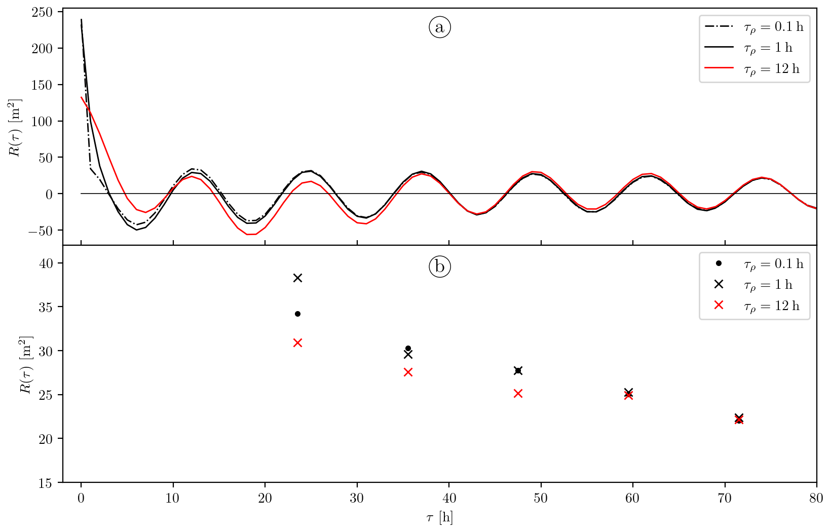
Figure B1 (a) Mean autocovariance computed from 1000 synthetic time series generated following the model Eq. (C8) for τ_ρ=0.1, 1, and 12 h (dash-dotted black, solid black, and solid red curve, respectively) and a fixed $S/N=\mathrm{0.2}$. (b) Complex demodulates at the semidiurnal frequency of the autocovariance series shown in (a).

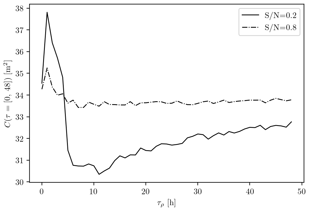
Figure B2 First 48 h demodulate of the mean autocovariance computed from 1000 synthetic time series generated following the model Eq. (B2) as a function of τ_ρ for fixed $S/N=\mathrm{0.2}$ (solid curve) and 0.8 (dash-dotted curve).

We repeat the same experiment for τ_ρ ranging from 0 to 48 h and focusing on the effects of the noise on the first demodulate. In Fig. B2, we plot the first demodulate as a function of τ_ρ (solid curve). For any τ_ρ, the first demodulate is seen to remain lower than the true ${\mathit{\sigma }}_{\mathrm{SD}}^{\mathrm{2}}=\mathrm{40}$ m². Moreover, two regimes can be identified: (i) for τ_ρ shorter than 5 h, roughly, the contribution of the non-tidal variability to the first demodulate is positive and peaks for τ_ρ=1 h, where $C(\mathit{\tau }=[\mathrm{0},\mathrm{48}\left]\right)\approx \mathrm{38}$ m², and (ii) for longer τ_ρ, this contribution is negative, with a minimum $C(\mathit{\tau }=[\mathrm{0},\mathrm{48}\left]\right)\approx \mathrm{30}$ m² at τ_ρ=11 h. For a more typical $S/N=\mathrm{0.8}$, i.e., setting ${\mathit{\sigma }}_{\mathit{\rho }}^{\mathrm{2}}=\mathrm{50}$ m² in our synthetic time series, we found a similar dependence of the first demodulate on τ_ρ as previously but with a much smaller span in amplitude (dash-dotted curve in Fig. B2). The contribution of the non-tidal variability to the first demodulate again peaks for τ_ρ=1 h, with $C(\mathit{\tau }=[\mathrm{0},\mathrm{48}\left]\right)\approx \mathrm{35}$ m², and the minimum occurs around τ_ρ=8 h, where $C(\mathit{\tau }=[\mathrm{0},\mathrm{48}\left]\right)\approx \mathrm{33}$ m².

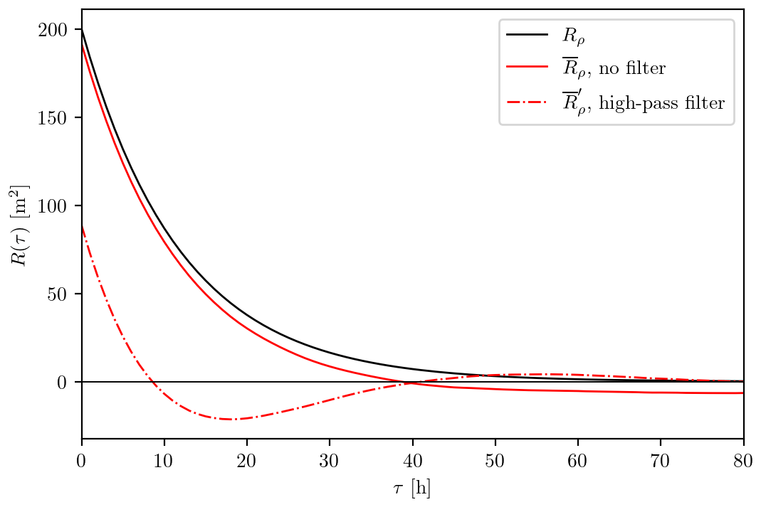
Figure B3 Theoretical autocovariance of the AR1 process ρ(t) with τ_ρ=12 h and ${\mathit{\sigma }}_{\mathit{\rho }}^{\mathrm{2}}=\mathrm{200}$ m² (solid black curve) and sample mean autocovariance computed from 1000 non-filtered and 1000 high-pass-filtered synthetic time series of ρ(t) (solid and dash-dotted red curve, respectively), constructed using the same parameters.

Figure B4 First 48 h demodulate of the mean autocovariance computed from 1000 synthetic time series generated following the model Eq. (B2) as a function of $S/N$ for fixed τ_ρ=1 (solid black curve) and 12 h (solid red curve). The first demodulates of the corresponding noise-corrected autocovariances are shown as the black and red dash-dotted curves, for τ_ρ=1 and 12 h, respectively.

Hence, for the typical $S/N=\mathrm{0.8}$ and τ_ρ=1 observed by Argo floats, we estimate that the non-tidal variability can lead to a first demodulate being biased high by roughly 3 %. For the same characteristic timescale but $S/N=\mathrm{0.2}$ (the 5th percentile of the global $S/N$ distribution sampled by Argo floats), this bias can reach 10 %. Notwithstanding, even for such an extreme $S/N$ value, the first demodulate is seen to remain a conservative estimate of the IT variance. The effects of the non-tidal variability on the IT variance estimate as computed in Geoffroy and Nycander (2022) thus do not put their results into question.

It is not straightforward to understand why the contribution of the non-tidal variability to the value of the first demodulate can be negative. Because of the way we defined ρ(t), i.e., an AR1 process with a positive parameter, its autocovariance should remain positive. Oscillations of R_ρ(τ) are actually a consequence of the high-pass filter applied to the time series. We show this in Fig. B3, where we plot the theoretical autocovariance of ρ(t) with τ_ρ=12 h and ${\mathit{\sigma }}_{\mathit{\rho }}^{\mathrm{2}}=\mathrm{200}$ m² (solid black curve) and the sample mean autocovariance from 1000 non-filtered and 1000 high-pass-filtered synthetic time series (solid and dash-dotted red curve, respectively) constructed using the same parameters.

As mentioned in Sect. 3.2, we expect the stochastic background noise affecting the simulated data to be different from the one recorded by the in situ instruments. Therefore, to prevent any systematic bias in the comparisons presented in this work, we consistently correct the sample autocovariance by subtracting an estimate of the autocovariance of the non-tidal variability before performing the complex demodulation (see Appendix C). We illustrate the effects of this correction in Fig. B4. Here, we proceed in the same way as for Fig. B2, but this time varying $S/N$ (from $\mathrm{4}\times {\mathrm{10}}^{-\mathrm{2}}$ to 4) for fixed τ_ρ=1 and 12 h. While the first demodulates of the non-corrected mean autocovariances diverge for small $S/N$ values (solid curves), the first demodulates of the noise-corrected autocovariances are virtually constant (dash-dotted curves).

Appendix C: Estimating the autocovariance of the non-tidal variability

In the present appendix, we derive a model for the autocovariance of a tidal variability on top of a high-pass-filtered stochastic noise. In Appendix B we show that the autocovariance of the non-tidal variability is affected by the high-pass filter we apply on the original time series (see Fig. B3). This consequence of filtering the time series was not taken into account by Geoffroy and Nycander (2022) in the model of the background noise they used.

Assume that the non-tidal variability ρ(t) is a first-order autoregressive process (AR1) characterized by zero mean, the timescale τ_ρ, and the white Gaussian noise ε_ρ(t) with zero mean and variance ${\mathit{\sigma }}_{\mathit{\epsilon },\mathit{\rho }}^{\mathrm{2}}$. In the time domain, the filtered ρ^′(t) can be modeled as the convolution of the unfiltered ρ(t) with the impulse response of the filter h(t). We are, however, interested in the autocovariance of ρ^′(t), $R_{\mathit{\rho }}^{\prime }\left(\mathit{\tau }\right)$, which is closely related to the power spectrum (one is the Fourier transform of the other). Luckily, it is much simpler to perform this operation in the frequency domain, where the power spectrum at the output of a linear filter, ${\mathcal{P}}_{\mathit{\rho }}^{\prime }\left(z\right)$, is related to the power spectrum of the input stochastic process, 𝒫_ρ(z), by

$$\begin{array}{}\text{(C1)}& {\mathcal{P}}_{\mathit{\rho }}^{\prime }\left(z\right)={\left|H\left(z\right)\right|}^{\mathrm{2}}{\mathcal{P}}_{\mathit{\rho }}\left(z\right).\end{array}$$

Here, H(z) is the system or transfer function of the filter, and the z domain is limited to the unit circle z=exp (jωΔt); i.e., the z transform is equivalent to the discrete Fourier transform, where ω is the angular frequency, and Δt is the constant sampling interval (Kay and Marple, 1981). Moreover, the power spectrum of an AR1 process is a standard result:

$$\begin{array}{}\text{(C2)}& {\mathcal{P}}_{\mathit{\rho }}\left(\mathit{\omega }\right)={\displaystyle \frac{{\mathit{\sigma }}_{\mathit{\epsilon },\mathit{\rho }}^{\mathrm{2}}\mathrm{\Delta }t}{\mathrm{1}+\exp (-\mathrm{2}/{\mathit{\tau }}_{\mathit{\rho }})-\mathrm{2}\exp (-\mathrm{1}/{\mathit{\tau }}_{\mathit{\rho }})\cos \left(\mathit{\omega }\mathrm{\Delta }t\right)}}.\end{array}$$

The Butterworth filter is linear in amplitude but not in phase. As a workaround, we applied a second-order filter twice, once forward and once backward, to recover a fourth-order filter with zero phase. The transfer function of a second-order high-pass Butterworth filter in the z domain, H_B2(z), can be obtained from its Laplace transform:

$$\begin{array}{}\text{(C3)}& H_{\mathrm{B}\mathrm{2}}\left(s\right)={\displaystyle \frac{\mathrm{1}}{({\mathit{\omega }}_{\mathrm{c}}/s{)}^{\mathrm{2}}+\sqrt{\mathrm{2}}({\mathit{\omega }}_{\mathrm{c}}/s)+\mathrm{1}}},\end{array}$$

where ω_c is the cut-off angular frequency (Schlichthärle, 2000). We use the bilinear transform, namely setting

$$\begin{array}{}\text{(C4)}& s={\displaystyle \frac{\mathrm{1}}{\mathrm{\Delta }t}}\ln \left(z\right)\approx {\displaystyle \frac{\mathrm{2}}{\mathrm{\Delta }t}}{\displaystyle \frac{z-\mathrm{1}}{z+\mathrm{1}}}\end{array}$$

in Eq. (C3), to recover the expression

$$\begin{array}{}\text{(C5)}& H_{\mathrm{B}\mathrm{2}}\left(z\right)={\displaystyle \frac{\mathrm{4}-\mathrm{8}{z}^{-\mathrm{1}}+\mathrm{4}{z}^{-\mathrm{2}}}{\begin{array}{c}({\mathit{\omega }}_{\mathrm{c}}^{\mathrm{2}}\mathrm{\Delta }{t}^{\mathrm{2}}+\mathrm{2}\sqrt{\mathrm{2}}{\mathit{\omega }}_{\mathrm{c}}\mathrm{\Delta }t+\mathrm{4})\\ +(\mathrm{2}{\mathit{\omega }}_{\mathrm{c}}^{\mathrm{2}}\mathrm{\Delta }{t}^{\mathrm{2}}-\mathrm{8})z^{-\mathrm{1}}\\ +({\mathit{\omega }}_{\mathrm{c}}^{\mathrm{2}}\mathrm{\Delta }{t}^{\mathrm{2}}-\mathrm{2}\sqrt{\mathrm{2}}{\mathit{\omega }}_{\mathrm{c}}\mathrm{\Delta }t+\mathrm{4})z^{-\mathrm{2}}\end{array}}}.\end{array}$$

Hence, we can evaluate Eq. (C1) as

$$\begin{array}{}\text{(C6)}& {\mathcal{P}}_{\mathit{\rho }}^{\prime }\left(\mathit{\omega }\right)=\left({\left|H_{\mathrm{B}\mathrm{2}}(z=\exp (j\mathit{\omega }\mathrm{\Delta }t\left)\right)\right|}^{\mathrm{2}}{)}^{\mathrm{2}}{\mathcal{P}}_{\mathit{\rho }}\right(\mathit{\omega }).\end{array}$$

Since ρ^′ is real-valued, the autocovariance $R_{\mathit{\rho }}^{\prime }\left(\mathit{\tau }\right)$ is given by the inverse discrete Fourier cosine transform of its power spectrum ${\mathcal{P}}_{\mathit{\rho }}^{\prime }\left(\mathit{\omega }\right)$ (computed numerically).

As mentioned in Sect. 3.2, to limit any systematic bias we consistently estimate and subtract the autocovariance of the non-tidal variability from the sample autocovariance before performing the complex demodulation. We obtain such an estimate from the least squares fit of the model adapted from Geoffroy and Nycander (2022),

$$\begin{array}{}\text{(C7)}& \begin{array}{rl}{R}_m\left(\mathit{\tau }\right)& =R_{{\mathit{\rho }}_{\mathrm{f}}}^{\prime }\left(\mathit{\tau }\right)+R_{{\mathit{\rho }}_{\mathrm{s}}}^{\prime }\left(\mathit{\tau }\right)\\ & +\sum _i{\displaystyle \frac{A_i}{\mathrm{2}}}\cos \left({\mathit{\omega }}_i\mathit{\tau }\right)\exp (-{\mathit{\sigma }}_{\mathit{\varphi },i}^{\mathrm{2}}+R_{\mathit{\varphi },i}(\mathit{\tau }\left)\right),\end{array}\end{array}$$

corresponding to the autocovariance of a tidal variability affected by a background noise:

$$\begin{array}{}\text{(C8)}& m\left(t\right)={\mathit{\rho }}_{\mathrm{f}}^{\prime }\left(t\right)+{\mathit{\rho }}_{\mathrm{s}}^{\prime }\left(t\right)+\sum _i{A}_i\cos ({\mathit{\omega }}_{i}t+{\mathit{\varphi }}_i(t\left)\right).\end{array}$$

Here, ω_i and A_i are the angular frequency and the amplitude of the tidal constituent i, respectively, where $i\in [M_{\mathrm{2}},S_{\mathrm{2}},K_{\mathrm{1}},O_{\mathrm{1}}]$. ϕ_i(t) is an AR1 process representing the random phase modulations affecting the constituent i. For the sake of simplicity, we assume that the decorrelating processes act in the same manner on neighboring tidal frequencies, that is, ${\mathit{\varphi }}_{M_{\mathrm{2}}}\left(t\right)={\mathit{\varphi }}_{S_{\mathrm{2}}}\left(t\right)$ and ${\mathit{\varphi }}_{K_{\mathrm{1}}}\left(t\right)={\mathit{\varphi }}_{O_{\mathrm{1}}}\left(t\right)$. Note that the high-pass filter used in this work was designed so as not to affect the tidal signal. ${\mathit{\rho }}_{\mathrm{f}}^{\prime }\left(t\right)$ and ${\mathit{\rho }}_{\mathrm{s}}^{\prime }\left(t\right)$ are high-pass-filtered AR1 processes accounting for a fast and a slow non-tidal variability, respectively. All the AR1 processes are characterized by zero mean, the timescale τ_X, and the white Gaussian noise ε_X(t) with zero mean and variance ${\mathit{\sigma }}_{\mathit{\epsilon },X}^{\mathrm{2}}$, where $X\in [\mathit{\varphi },{\mathit{\rho }}_{\mathrm{f}},{\mathit{\rho }}_{\mathrm{s}}]$. The variance and autocovariance of an AR1 process are

$$\begin{array}{}\text{(C9)}& {\mathit{\sigma }}_X^{\mathrm{2}}={\displaystyle \frac{{\mathit{\sigma }}_{\mathit{\epsilon },X}^{\mathrm{2}}}{\mathrm{1}-\exp (-\mathrm{2}/{\mathit{\tau }}_X)}},R_X\left(\mathit{\tau }\right)={\mathit{\sigma }}_X^{\mathrm{2}}\exp (-\mathit{\tau }/{\mathit{\tau }}_X),\end{array}$$

respectively. The model Eq. (C7) does not take into account the effects of the drift of the floats or Lagrangian particles.

Figure C1 (a) Atlas of the semidiurnal IT variance at 1000 dbar computed from the fitting of the model Eq. (C7) to the same local-mean autocovariance series as used in Fig. 6c. (b) Non-tidal variance from the same fitting as in (a). (c) Signal-to-noise ratio computed as the ratio of (a) over (b). The ocean mask is colored in yellow for readability.

We fit the full model Eq. (C7), containing 12 parameters, to the sample autocovariance by nonlinear least squares, with weights inversely proportional to the corresponding SEM, and imposed bounds on the parameters (since we only fit positive timescales and variances). In particular, the timescales of the fast and slow non-tidal variability are restricted to the [0, 5] and [5, 48] h range, respectively. The autocovariance of the non-tidal variability is then computed as

$$\begin{array}{}\text{(C10)}& R_{\mathit{\rho }}^{\prime }\left(\mathit{\tau }\right)=R_{{\mathit{\rho }}_{\mathrm{f}}}^{\prime }\left(\mathit{\tau }\right)+R_{{\mathit{\rho }}_{\mathrm{s}}}^{\prime }\left(\mathit{\tau }\right)\end{array}$$

using the fitted parameters. Lastly, $R_{\mathit{\rho }}^{\prime }\left(\mathit{\tau }\right)$ is subtracted from the sample autocovariance to correct for the effects of the filtered background noise.

The inclusion of a tidal variability in the model Eq. (C7) primarily aims at limiting the projection of the observed tidal variability onto our model for the background noise when fitting. Nonetheless, the fitted parameters can be used to compute an estimate of the semidiurnal IT variance ${\mathit{\sigma }}_{\mathrm{SD},\mathrm{LS}}^{\mathrm{2}}=(A_{M_{\mathrm{2}}}^{\mathrm{2}}+A_{S_{\mathrm{2}}}^{\mathrm{2}})/\mathrm{2}$ and further to estimate the signal-to-noise ratio characterizing the filtered Argo records as $S/N={\mathit{\sigma }}_{\mathrm{SD},\mathrm{LS}}^{\mathrm{2}}/R_{\mathit{\rho }}^{\prime }\left(\mathrm{0}\right)$. In Fig. C1 we show maps of ${\mathit{\sigma }}_{\mathrm{SD},\mathrm{LS}}^{\mathrm{2}}$, $R_{\mathit{\rho }}^{\prime }\left(\mathrm{0}\right)$, and $S/N$ computed from the same collection of local-mean autocovariances as used in Fig. 6c. Note that ${\mathit{\sigma }}_{\mathrm{SD},\mathrm{LS}}^{\mathrm{2}}$ and $R_{\mathit{\rho }}^{\prime }\left(\mathrm{0}\right)$ are not correlated (r²=0.13 and 0.009 in the log–log and linear domain, respectively). The least-squares-fitted ${\mathit{\sigma }}_{\mathrm{SD},\mathrm{LS}}^{\mathrm{2}}$ appears reasonable when compared with the first demodulates presented in Fig. 6c. The coefficient of determination r²=0.53 and 0.29 in the log–log and linear domain, respectively, indicates a good agreement between the two estimates. Moreover, the global mean and median of their ratio are 0.8 and 0.7, respectively, accounting for the decorrelation of the IT taking place in the first 48 h. For such local-mean autocovariances, however, the uncertainties are simply to high to reliably estimate the parameters of the decorrelating process ϕ_i(t). Finally, we chose to perform the comparisons presented in this work in terms of the first demodulate, for it is a conservative and more robust estimate of the IT variance.