Improving sea surface temperature in a regional ocean model through refined sea surface temperature assimilation

Infrared (IR) and passive microwave (PMW) satellite sea surface temperature (SST) retrievals are valuable to assimilate into high-resolution regional ocean forecast models. Still, there are issues related to these SSTs that need to be addressed to achieve improved ocean forecasts. Firstly, satellite SST products tend to be biased. Assimilating SSTs from different providers can thus cause the ocean model to receive inconsistent information. Secondly, while PMW SSTs are valuable for constraining models during cloudy conditions, the spatial resolution of these retrievals is rather coarse. Assimilating PMW SSTs into high-resolution ocean models will spatially smooth the modeled SST and consequently remove finer SST structures. In this study, we implement a bias correction scheme that corrects satellite SSTs before assimilation. We also introduce a special observation operator, called the supermod operator, into the Regional Ocean Modeling System (ROMS) four-dimensional variational data assimilation algorithm. This supermod operator handles the resolution mismatch between the coarse observations and the finer model. We test the bias correction scheme and the supermod operator using a setup of ROMS covering the shelf seas and shelf break off Norway. The results show that the validation statistics in the modeled SST improve if we apply the bias correction scheme. We also find improvements in the validation statistics when we assimilate PMW SSTs in conjunction with the IR SSTs. However, our supermod operator must be activated to avoid smoothing the modeled SST structures on spatial scales smaller than twice the PMW SST footprint. Both the bias correction scheme and the supermod operator are easy to apply, and the supermod operator can easily be adapted for other observation variables.

1 Introduction

Satellite-based sea surface temperature (SST) retrievals account for the majority of observations assimilated into most ocean forecast models and can be retrieved by measuring both the infrared (IR) and passive microwave (PMW) radiation emitted by the ocean surface. Cloud coverage reduces the number of SST retrievals by IR sensors. Consequently, SSTs from PMW radiometers serve as a complementary data set as PMW radiation penetrates clouds. While the spatial resolution of IR SSTs is typically ∼ 1 km, which is similar to or finer than those of regional ocean forecast models (∼ 1–10 km), a disadvantage with PMW SSTs is their relatively coarse resolution. For the instrument AMSR-2 (Advanced Microwave Scanning Radiometer 2) on board GCOM-W1 (Global Change Observation Mission-Water 1), the elliptic PMW SST footprint is ∼ 35 × 62 km (Imaoka et al., 2010).

Indeed, mesoscale ocean models can resolve circulation features at smaller spatial scales than PMW SSTs can provide. Such differences in resolved scales are commonly referred to as representation errors within the field of data assimilation (Janjić et al., 2018). Previous studies have considered the differences in resolved scales while assimilating coarse observations such as those of sea ice concentration, satellite sea surface salinity, and scatterometer ocean surface winds (Buehner et al., 2013; Martin et al., 2019; Mile et al., 2021). In these studies, the observation operator was modified such that the coarse observations could be compared with the average of the model values located within an area similar to the spatial resolution of the observations. Similar ideas for the observation operator have also been applied while producing global SST analyses where IR and PMW SSTs are merged using statistical methods (Donlon et al., 2012; Brasnett and Colan, 2016). However, as far as the authors are aware, such an observation operator has not been described and implemented for the assimilation of PMW SSTs into a high-resolution regional ocean forecast model.

To tackle the mismatch in spatial resolution, we implement an observation operator, called the supermod operator, into the Regional Ocean Modeling System (ROMS; Haidvogel et al., 2008; Shchepetkin and McWilliams, 2009) four-dimensional variational (4D-Var) data assimilation system (Moore et al., 2011; Gürol et al., 2014). This operator considers the resolution mismatch between the PMW SSTs and the model by comparing each PMW SST observation with the model mean over an area similar to the observation footprint. The implementation of the operator follows a similar methodology as described in Mile et al. (2021). We show that, compared to a traditional observation operator, the supermod operator prevents PMW SSTs from constraining the spatial scales of the model that the PMW SSTs do not resolve properly. Thus, the supermod operator enables us to assimilate PMW SSTs without smoothing the modeled SST structures. We test the operator using a configuration of ROMS that covers the shelf seas and shelf break off Norway. This region is subject to high cloud coverage, meaning that there is a need for assimilating PMW SSTs to better constrain the model. Also, the Rossby radius of deformation, which affects the horizontal scales of mesoscale processes, decreases with increasing latitude. Consequently, SST structures arising from mesoscale processes are typically smaller at high latitudes, which leads to a greater risk of smoothing the modeled SST in these regions when assimilating coarse PMW SSTs.

To further improve the modeled SST, we take into account that satellite SSTs from different providers tend to be biased due to differences and limitations in the SST retrieval processes and algorithms (Chan and Gao, 2005; Høyer et al., 2012; Wang et al., 2016). Specifically, we implement a bias correction scheme which is inspired by Høyer et al. (2014) and use this scheme to correct the assimilated satellite SSTs for biases. The scheme ensures consistency between SST observations from different providers, thus preventing the model from receiving inconsistent information during the assimilation of different products. By reducing inconsistencies, the probability of artificial noise in the modeled SST is reduced.

2 Data and methods

2.1 Model configuration and data assimilation setup

ROMS is a free-surface, hydrostatic, primitive-equation ocean model using stretched, terrain-following vertical coordinates, which is beneficial for modeling shallow, coastal waters. The model domain used in this study covers the shelf seas and shelf break off Norway (Fig. 1). We present only a brief summary of the model configuration, since a thorough description can be found in Röhrs et al. (2018).

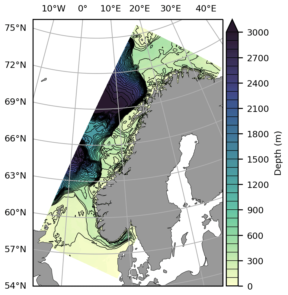
Figure 1 Bathymetry of the model region covering the shelf seas and shelf break off Norway.

The model domain has a horizontal resolution of 2.4 km, and there are 42 layers in the vertical direction, which are distributed so that the uppermost layer has a thickness of ∼ 0.2–1.2 m. Vertical mixing is parameterized using a second-order scheme for turbulent kinetic energy and a generic length scale based on a setup recommended by Umlauf and Burchard (2005) and Warner et al. (2005). The configuration differs slightly from that of Röhrs et al. (2018), with different choices for the K_min and P_min parameters, which in our case are set to 1.0 × 10⁻⁸.

We force the model with 3-hourly operational forecast data from the Integrated Forecast System of the European Centre for Medium-Range Weather Forecasts (ECMWF, 2016). Air–sea fluxes for momentum and heat are calculated via the COARE3.0 bulk flux algorithms (Fairall et al., 2003) within ROMS. Open boundary conditions consist of daily averages of all state variables from the TOPAZ4 reanalysis (Xie et al., 2017). As TOPAZ4 does not include the inverse barometer effect, the sea surface elevation and currents are adjusted to include the effect of local atmospheric pressure. Harmonic tidal forcing, consisting of eight tidal constituents from the TPXO9 global inverse barotropic model (Egbert and Erofeeva, 2002), is also imposed along the open boundaries. Riverine runoff is based on modeled river discharges from the Norwegian Water Resources and Energy Directorate (Beldring et al., 2003).

The model is initialized from the TOPAZ4 reanalysis on 1 January 2017 and run with 4D-Var assimilation of satellite SST and in situ temperature and salinity observations, as described in Röhrs et al. (2018). This reanalysis is used to initialize a set of different experiments (see Sect. 4.1), all of which assimilate only satellite SST observations and are run for the period 21 April 2018–22 June 2018.

The assimilation algorithm used for the experiments is the dual formulation of the ROMS 4D-Var system (RBL4DVAR; Moore et al., 2011; Gürol et al., 2014). Generally, in 4D-Var data assimilation, the analysis is found by minimizing a cost function in the following form:

$$\begin{array}{}\text{(1)}& \begin{array}{rl}J\left(\mathit{x}\right)& ={\displaystyle \frac{\mathrm{1}}{\mathrm{2}}}(\mathit{x}-{\mathit{x}}^{\mathrm{b}}{)}^T{\mathbf{B}}^{-\mathrm{1}}(\mathit{x}-{\mathit{x}}^{\mathrm{b}})\\ & +{\displaystyle \frac{\mathrm{1}}{\mathrm{2}}}{\left(\mathit{y}-\mathcal{H}\left(\mathit{x}\right)\right)}^T{\mathbf{R}}^{-\mathrm{1}}(\mathit{y}-\mathcal{H}(\mathit{x}\left)\right),\end{array}\end{array}$$

where the control vector, x, holds the control variables, which include the prognostic variables (temperature, salinity, horizontal velocity, and sea surface height) at the model grid points. The background control vector is denoted x^b, while the vector y contains the observations. The observation operator, ℋ, returns the model equivalents of the observations by interpolating the model values to the observation locations. In case the observed quantity is not part of the control vector, ℋ may also transform the model values to correspond to the observed quantity. In 4D-Var, the nonlinear model is a part of ℋ and facilitates temporal mapping. B is the background error covariance matrix, while R is the observation error covariance matrix. R is assumed to be diagonal in most operational data assimilation systems, including the implementation in ROMS used in this study (Gürol et al., 2014). This assumption means that the observation errors are assumed to be uncorrelated in both time and space. The observation errors used to construct R include both the measurement error, which is the error associated with the accuracy of the measuring instrument, and the representation errors (Janjić et al., 2018). Following Janjić et al. (2018), the latter is connected to errors arising from the pre-processing and quality control of the observations, the observation operator, and the mismatch between the resolutions of the observations and the model grid.

In ROMS, the construction of the background error covariance matrix B follows the approach described in Weaver and Courtier (2001), where B is separated into a univariate correlation matrix, a multivariate balance operator, and background error standard deviations. The background error standard deviations are, in this study, calculated from a multi-year simulation with the same model configuration. To avoid unrealistically high values of the standard deviations due to large seasonal variations, background standard deviations are calculated separately for each day of the year, using all of the time records in the multi-year run that fall within ±14 d of the day in question. Consequently, the B used in this study changes slightly from one assimilation cycle to the next. We do not apply any explicit balance relations between the control variables. However, the linearized physics in the tangent-linear and adjoint models implicitly account for correlations between the control variables.

The standard deviation of the error attributed to an observation (σ_o) is estimated as a function of the background error standard deviation at the observation location (σ_b), a factor based on the reported quality level of the satellite products (Q), and a parameter α as follows:

$$\begin{array}{}\text{(2)}& {\mathit{\sigma }}_{\mathrm{o}}^{\mathrm{2}}=\mathit{\alpha }\cdot Q\cdot {\mathit{\sigma }}_{\mathrm{b}}^{\mathrm{2}}.\end{array}$$

The reported quality level reflects the uncertainty of the observation and is assigned to each SST measurement by the data creator (Donlon et al., 2007). Only quality level 4 (QL4 – acceptable quality) and 5 (QL5 – best quality) are used. To ensure that more weight is given to the observations with the best quality during assimilation, observations with QL4 and QL5 are assigned a Q of 1.1 and 0.9, respectively. The parameter α is set to α=2 for all of the satellite products to ensure that the different experiments are comparable, and it is chosen by validating a set of experiments with different choices of α against independent data sets.

2.2 Observations

We use satellite SST observations from IR and PMW radiometers, and a summary of the products is found in Table 1. All observations are level-2 preprocessed (L2P) products downloaded from the Physical Oceanography Distributed Active Archive Center (PO.DAAC), the Satellite Application Facility on Ocean and Sea Ice (OSI SAF) FTP server, and the European Organisation for the Exploitation of Meteorological Satellites (EUMETSAT) data center online ordering client.

Table 1 IR and PMW satellite SST observations used in this study and their approximate spatial resolution at nadir.

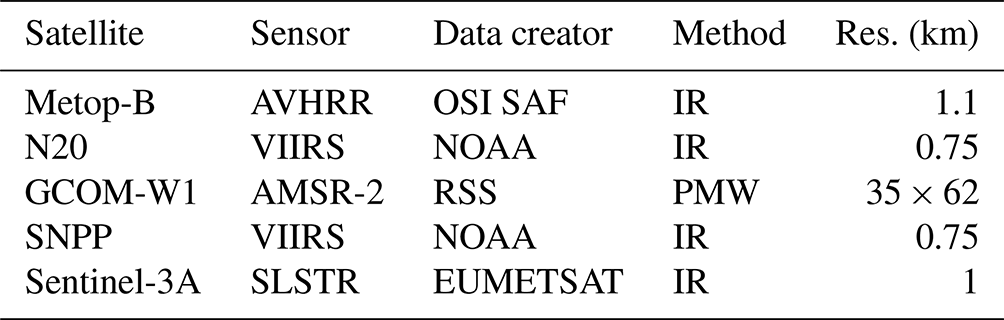
The IR SSTs have a spatial resolution ranging from 0.75–1.1 km at nadir and are thus capable of resolving SST structures of similar scales as the structures captured by the model. When several of these observations fall within the same model grid cell during the same time interval, the mean of the observations is calculated to create a super-observation. In our setup, each individual observation time is rounded to the nearest quarter hour before super-observations are calculated.

PMW radiometers can, unlike IR radiometers, retrieve SSTs during cloudy conditions. Challenges related to PMW SST retrievals that require affected pixels to be discarded include rain, radio frequency inference, sun glint, and emission from sea ice surfaces and land (Minnett et al., 2019). The latter contamination affects PMW retrievals from regions within ∼ 100 km from land. The spatial resolution of PMW SSTs depends on the frequency used to derive the SSTs along with the antenna size and is significantly coarser than those of the IR SSTs. For AMSR-2 GCOM-W1, the primary band for PMW SST retrieval at 6.9 GHz corresponds to an elliptic footprint, elongated in the along-track direction of the satellite, with sizes of approximately 35 × 62 km (Imaoka et al., 2010).

All satellite SST observations are corrected by applying the single-sensor error statistics (SSES) bias, in line with the recommendations in Donlon et al. (2007). As previously mentioned, we use QL4 and QL5 for the assimilated IR SST products. For the PMW SSTs, we use only QL5 observations and discard the QL4 observations due to unwanted artifacts in the SST field. These artifacts are likely caused by radio frequency interference from oil rigs (Alerskans et al., 2020). Evaluation of the QL5 PMW SSTs revealed that observations of dubious quality are still present in the data set, both at the edges of areas from which low-quality observations were removed and in areas corresponding to locations of oil rigs. Thus, an additional quality control of the PMW SSTs was implemented, flagging observations as bad if they are within a radius of 75 km of an oil rig.

The SLSTR (Sea and Land Surface Temperature Radiometer) instrument on board Sentinel-3A uses a dual-view technique where the swath is scanned twice through two different atmospheric path lengths. This capability allows for more accurate SST measurements (Luo et al., 2020). We use QL5 SSTs measured by this sensor to correct the other satellite products for biases (see Sect. 2.3) and for validation purposes. Other SSTs used for validation are bias-corrected SSTs from VIIRS (Visible Infrared Imaging Radiometer Suite) SNPP (Suomi National Polar-orbiting Partnership) and SSTs measured by drifting buoys from the CORA data set (Cabanes et al., 2013). The spatial coverage of the drifting buoys is shown in Fig. 2.

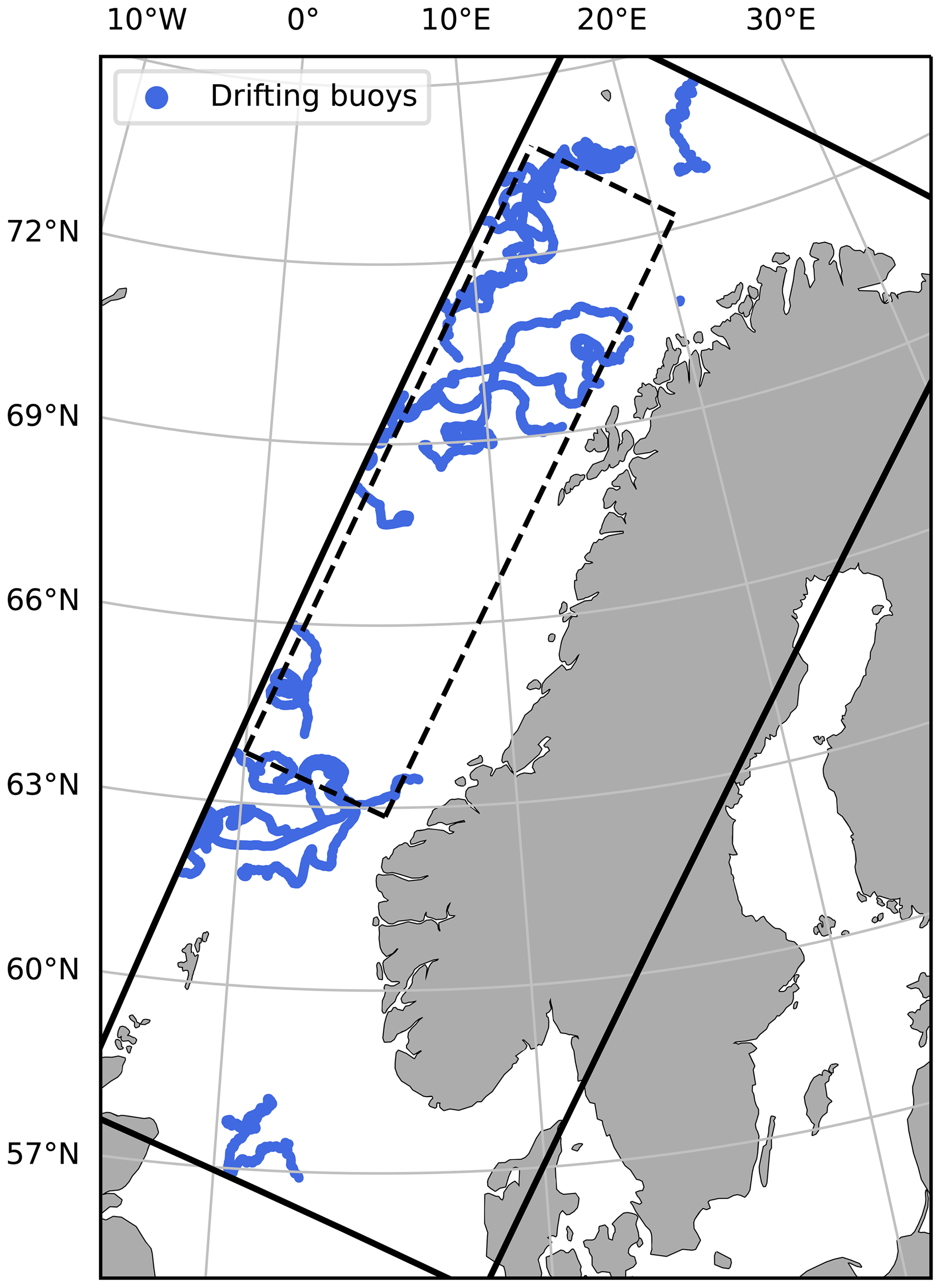
Figure 2 Spatial coverage of CORA drifting buoys during the period 27 April 2018–22 June 2018, which is the period used for validation. There are in total ∼ 10 600 observations of this kind. The solid black box shows the extent of the model domain, while the dashed black box shows the domain selected for SST power spectrum calculations (see Sect. 4.3).

While SLSTR Sentinel-3A provides the skin temperature, the other satellite products used in this study provide the sub-skin temperature. IR sensors intrinsically measure the skin temperature. However, these skin temperatures are converted to sub-skin temperatures during the data creation process if in situ data are used to tune parameters included in the SST retrieval algorithms. To ensure that all of the SSTs used throughout this study represent the sub-skin temperature, an offset of 0.17 ^∘C is added to the SLSTR Sentinel-3A SSTs (Donlon et al., 2002; Høyer et al., 2014). This constant offset is generally valid for wind speeds above 6 m s⁻¹ but may be greater for lower wind speeds. Our results indicate, however, that using this constant offset to convert the SLSTR Sentinel-3A SSTs to sub-skin temperatures does not degrade the modeled SST resulting from assimilating bias-corrected SSTs (see Sect. 4.2).

Figure 3 shows time series of the number of observations inside the model domain during the chosen assimilation period in 2018. For the satellite observations, we count only observations that meet the set minimum quality level. Cloudiness causes the number of IR SST observations to vary. The largest number of observations occurs at the beginning of May, and there is a drop in the number of available observations while approaching June. The number of PMW SST observations is stable during the whole period, which we expect, since PMW SSTs can be measured in cloudy conditions. Moreover, the number of available PMW SSTs is, on average, smaller than the number of available IR SSTs, since the PMW SSTs are provided on a coarser grid.

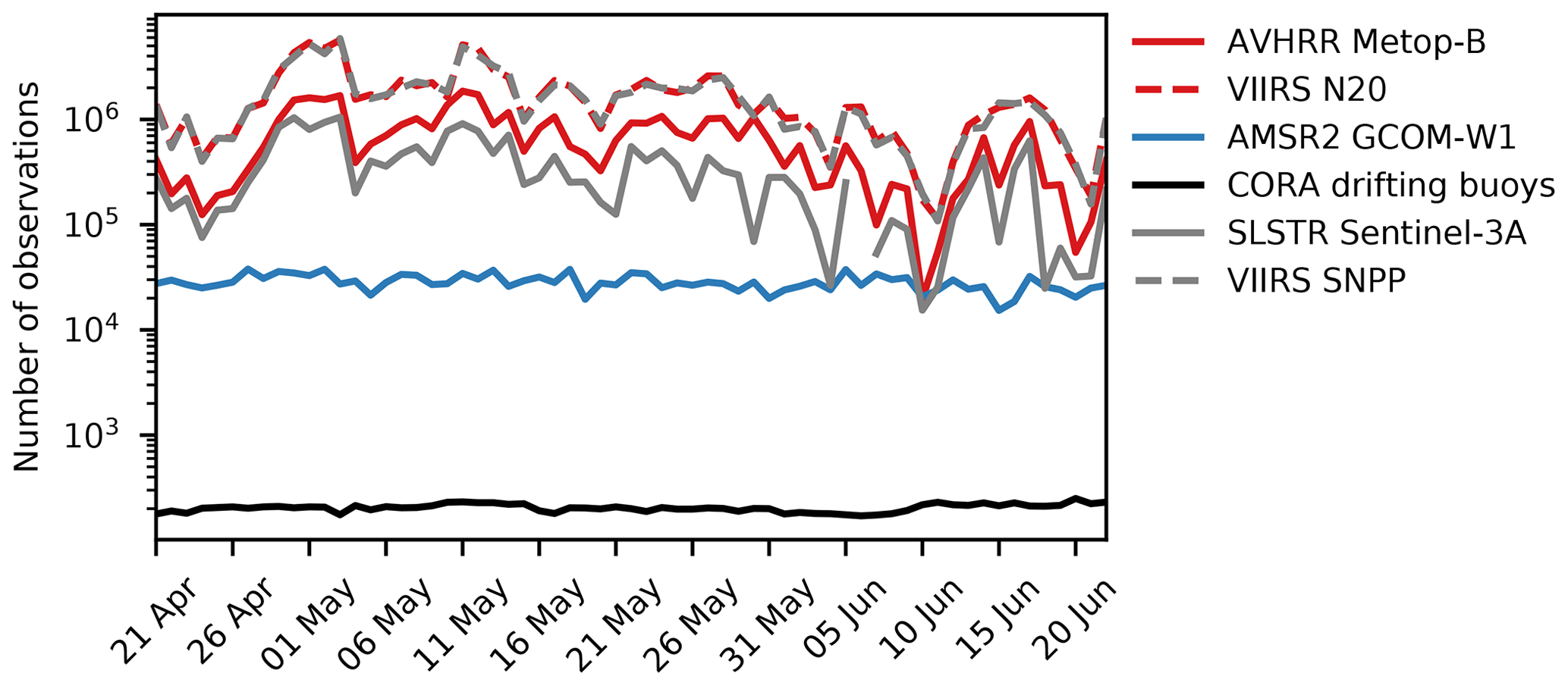
Figure 3 Time series of the number of observations per day available inside the model domain for each sensor and satellite pair and for the CORA drifting buoys.

2.3 SST bias correction algorithm

High northern latitudes are recognized as challenging regions for satellite SST retrieval (Donlon et al., 2010; Wang et al., 2016; Jia and Minnett, 2020). In situ data are used to derive the satellite SST retrieval algorithms and to correct and thus improve the quality of the retrieved SST. However, the number of available in situ SST measurements at high northern latitudes is low compared to equatorial and mid-latitude regions, and this data scarcity can lower the quality of high-latitude IR and PMW SST retrievals (O’Carroll et al., 2019).

SST retrievals in the IR are subject to additional challenges. First, the process of cloud screening, where cloudy and clear-sky conditions are separated, is critical (O’Carroll et al., 2019). Any undetected clouds will result in erroneous SST retrievals. Additionally, the brightness temperatures derived from the measured IR radiances are modified by aerosols and gases, such as water vapor, in the atmosphere. Atmospheric correction algorithms are thus required to retrieve accurate SSTs. At high latitudes, these corrections tend to be problematic, thereby degrading the accuracy of the measured SSTs (Kumar et al., 2003; Merchant et al., 2006; Vincent, 2018; Jia and Minnett, 2020).

For the PMW part of the spectrum, challenges that must be corrected for (in addition to those mentioned in Sect. 2.2, which cause the measurements to be discarded) include sea surface roughness generated from strong winds and atmospheric effects such as those associated with modification of the PMW radiation by water vapor and liquid water (Wentz et al., 2000; Minnett, 2014).

SST products from various satellites and sensors are subject to regional and temporal biases due to the difficulties concerning the SST retrieval process and the differences in applied retrieval algorithms (Chan and Gao, 2005; Høyer et al., 2012; Wang et al., 2016). To this end, Høyer et al. (2014) developed and employed a bias correction scheme that they used to correct SST products from different providers. Their goal was to merge these products, and the correction was performed to prevent any biases from affecting the final product. Bias correction schemes have also been implemented in other studies in order to correct the satellite SSTs being assimilated into ocean models. For example, Waters et al. (2015) employed a scheme where SSTs were corrected using a set of chosen reference observations. This bias correction was performed prior to the assimilation of the observations. While and Martin (2019), on the other hand, implemented a variational bias correction scheme where the SSTs were corrected within the data assimilation algorithm. In such variational schemes, bias correction is achieved by incorporating additional terms into the cost function. One key advantage of variational schemes is that they do not rely on having full coverage of reference observations at all times.

We implement a similar bias correction scheme as in Høyer et al. (2014), with some modifications, to ensure consistency between the different satellite SST products being assimilated into our model. The bias correction is an individual step during the preparation of observations for assimilation and is not part of the data assimilation process itself. Biases are calculated independently for all satellite products using SLSTR Sentinel-3A SST as reference. Figure 4 illustrates such a bias field for AVHRR (Advanced Very High Resolution Radiometer) Metop-B, and the method is described below.

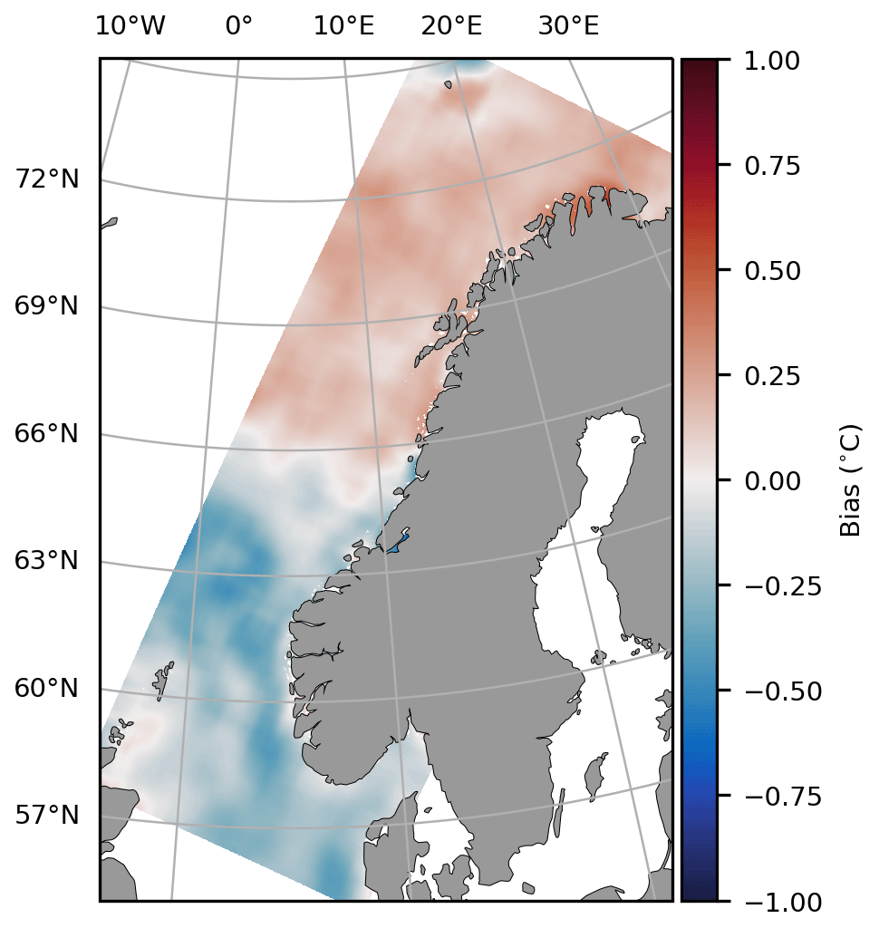
Figure 4 Bias for AVHRR Metop-B on 22 May 2018. The bias is calculated using 11 daily difference fields from 17 to 27 May 2018.

Daily SST fields on a grid with a resolution of ∼ 25 km are produced for each satellite product, including the reference product, by first resampling the available L2P SST products to this coarser grid and then calculating the mean of the observations falling into each grid cell. To minimize the possibility of using SST observations affected by greater diurnal warming events (Eastwood et al., 2011; Karagali et al., 2012), we exclude observations located in regions where the wind speed is less than 3 m s⁻¹ during local summer daytime (defined here as May–August at 10:00–14:00 UTC). This wind speed threshold is less strict than that recommended in Donlon et al. (2002) but was chosen to ensure sufficient spatial coverage in the daily fields, as the recommended threshold resulted in degraded bias estimates in cloudy regions. We do, however, find that the low threshold value of 3 m s⁻¹ performs slightly worse on the few occasions when our region is affected by diurnal warming. In the future, the wind speed threshold should be reassessed and adjusted, possibly in conjunction with a somewhat coarser analysis grid.

Daily difference fields are produced by subtracting the reference daily SST field from the daily SST fields of the other satellite products. We remove all of the values where the difference exceeds ±2 ^∘C. This data removal is performed to exclude unrealistic values which we detected along the coast and in regions affected by cloud contamination.

By aggregating 11 daily difference fields, we produce a bias that is valid on the central day. The aggregation is performed as a simple temporal averaging, as in Høyer et al. (2014). The biases are finally resampled to the model grid and, to avoid unwanted noise, are spatially smoothed by applying a uniform filter. This filter has the size of 40 grid points (∼ 96 km) in both horizontal directions.

3 Supermod operator

As noted, observations with higher spatial resolution than the model are combined into super-observations. This procedure reduces the representation errors, as information on smaller spatial scales than what the model is able to represent is smoothed. For the case of PMW SSTs, however, each observation represents an SST average over the area covered by its footprint. For AMSR-2 GCOM-W1, this footprint is roughly 375 times larger than the area of a grid cell in our model domain. Thus, we expect the model to contain potentially valuable information on finer spatial scales than what is present in the observations. If observations of this type were assimilated with a traditional observation operator that does not account for the observation footprints, we would expect large, spatially correlated representation errors (Liu and Rabier, 2002). Such errors are particularly problematic in data assimilation systems designed to handle uncorrelated observation errors.

An observation operator that ensures that each PMW SST observation is compared with a model mean over an area equivalent to the SST footprint is implemented in ROMS to avoid corrections of finer scales. The implementation of the operator follows a similar methodology as that described in Mile et al. (2021). We will refer to this operator as the supermod operator.

Our implementation of the supermod operator builds on the assumption that the observation footprints are squares with sides of length (1+2L)dx, where (1+2L) is the number of grid cells and dx is the horizontal resolution of the model. L can be set separately for each individual observation, which makes the operator easy to apply to new observation sources and different model configurations. As the center of the observation footprint may be located between model grid points, the supermod value is calculated as a weighted mean of the values in grid cells that fall completely or partially within the footprint area. The assigned interpolation weights are based on the fractional area of the grid cells that fall within the footprint. This is done to conserve the effective resolution of the supermod values and to ensure that the model footprint is centered at the observation location. Other factors that could affect the effective resolution of the supermod values are land points within the footprint or the extension of the footprint beyond the boundaries of the model domain. The operator is designed to reject observations with such footprint features. Figure 5 illustrates how the operator works.

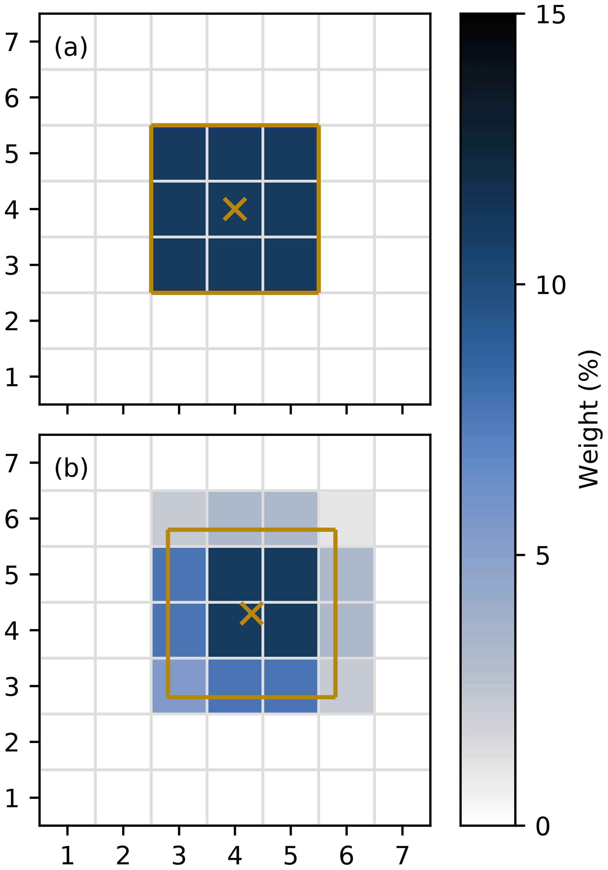
Figure 5 Schematic figure showing the supermod operator with L=1 for (a) an observation that falls exactly in the center of a model grid cell and (b) an observation that is shifted towards the upper right corner of a grid cell. The orange crosses indicate the observation locations, the mesh illustrates grid cells, and the orange squares indicate the footprint area of the observations. The color map indicates the weight (%) by which the grid cells contribute to the supermod value.

Idealized tests showed a sudden increase in the standard deviations of the innovations (observations minus background) when the footprints were increased and started to overlap. Thus, a thinning procedure is performed on the PMW observations prior to assimilating the observations. As the supermod operator can only represent square footprints, we have chosen L conservatively to ensure that the square used to represent the footprint will not be smaller than the largest size of the true, elliptic footprint of the satellite retrievals. With the grid resolution of our model being 2.4 km, L=13 gives us footprints with sides of 64.8 km. The PMW observations are thus thinned during a pre-processing step to ensure a distance of at least 64.8 km between the observation points.

3.1 Idealized experiment

An idealized scenario for a domain with flat bathymetry, no land, and no surface forcing is applied to test the behavior of the supermod operator in ROMS. A coarse grid with a horizontal resolution of ∼ 30 km is chosen to reduce the computational costs. The ocean is set to be initially at rest with a uniform temperature and salinity of 12 ^∘C and 34, respectively. The standard deviations of the background errors are also uniform for every prognostic variable, and it is set to 0.02 ^∘C for temperature.

A single PMW SST observation, with a temperature of 12.5 ^∘C and a standard deviation of the observation error set to be equal to the standard deviation of the background, is assimilated into the idealized setup for varying footprint sizes. Figure 6a–d show the resulting SST increments. Increasing the footprint size causes the increment to spread laterally, such that the observation affects a greater area. The increment amplitude decreases simultaneously. Furthermore, for each footprint size in Fig. 6a–d, we calculate the average increment using all values greater than zero (see white text in Fig. 6a–d). That the average increment remains relatively unchanged as the footprint size increases demonstrates that the inclusion of the supermod operator spreads the information from the PMW SST observation as expected.

Figure 6 SST increment for (a–d) varying sizes of L and with the observation error (${\mathit{\sigma }}_{\mathrm{o}}^{\mathrm{2}}$) set to be equal to the background error (${\mathit{\sigma }}_{\mathrm{b}}^{\mathrm{2}}$), (e) L=2 and ${\mathit{\sigma }}_{\mathrm{o}}^{\mathrm{2}}=\mathrm{1.5}{\mathit{\sigma }}_{\mathrm{b}}^{\mathrm{2}}$, and (f) L=2 and ${\mathit{\sigma }}_{\mathrm{o}}^{\mathrm{2}}=\mathrm{0.5}{\mathit{\sigma }}_{\mathrm{b}}^{\mathrm{2}}$.

Figure 6e and f show the effects of increasing and decreasing the observation error by a factor of 1.5 and 0.5, respectively, when the footprint parameter is set to L=2. Increasing (decreasing) the error decreases (increases) the increment amplitude, which is what we would expect. Further tests within this idealized framework revealed that the amplitude reduction with increasing L is not as pronounced when the observation error is set to be much smaller than the background error. In cases where the observation error is very small compared to the background error, the amplitude of the increment starts to increase with increasing L.

4 Results

4.1 Experimental design

Different experiments are set up to (1) test the effect of correcting satellite SSTs for biases before assimilation and (2) determine the effect of assimilating PMW SST observations with and without the application of the supermod operator. Table 2 summarizes the experiments, all of which cover the period 21 April 2018–22 June 2018.

Table 2 Summary of experiments showing the sources (sensor and satellite) of the assimilated satellite SSTs, whether the observations are corrected for biases through the bias correction scheme, whether the supermod operator is activated, and the approximate number of observations assimilated (∼ N_obs).

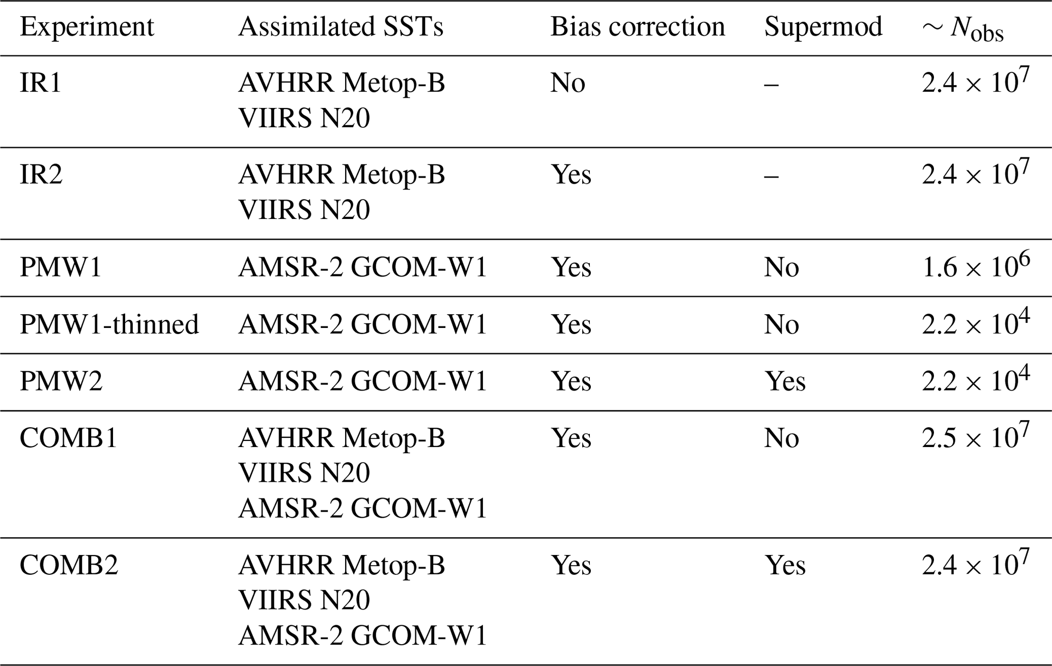
To assess the bias correction scheme, IR SSTs are assimilated with (IR2) and without (IR1) correcting for biases. Similarly, to assess the supermod operator, we assimilate PMW SSTs by first treating the SSTs as regular point observations (PMW1) and then by applying the supermod operator (PMW2). Notice that PMW2 includes the process of observation thinning. As a consequence, PMW2 assimilates only ∼ 1.4 % of the observations assimilated in PMW1. In order to separate the impact of the observation thinning from the impact of the supermod operator itself, we run an experiment where we assimilate a thinned set of the PMW SSTs without applying the supermod operator (PMW1-thinned). This experiment is essentially a thinned version of PMW1.

The argument for including PMW SSTs in the assimilated data set is to supplement the IR SSTs during periods of high cloud coverage. Hence, we run two additional experiments to determine the effects of combining IR and PMW SSTs. Experiment COMB1 assimilates IR and PMW SSTs without employing the supermod operator; i.e., the experiment is a combination of IR2 and PMW1. The final experiment, COMB2, is a combination of IR2 and PMW2, thus assimilating IR and PMW SSTs with the supermod operator activated.

The assimilation window is set to 3 d in all experiments. The assimilated observations update the background model state produced for such a 3 d cycle to produce the analysis. The ocean state at the end of the analysis is then used as initial conditions to produce the background state of the next assimilation cycle, and the process repeats. Thus, the background can be considered a forecast, and we evaluate the experiments using these background states in the following. The evaluation period excludes the two first assimilation cycles and covers 27 April 2018–22 June 2018. Note that the bias correction scheme is applied in all experiments but IR1.

4.2 Error statistics

Table 3 shows validation statistics of SST for the background states. PMW SST measurements are unavailable in the coastal zone, as emissions from land contaminate the retrievals in this region. The experiments assimilating only PMW SSTs thus perform quite poorly in these regions compared to the experiments that include IR SSTs. To assess the experiments, we have chosen to exclude observations within these areas from the validation, and we focus instead on the regions where an impact from including PMW SST can be expected.

In comparing IR1 and IR2, we find that correcting the observations for biases reduces the RMSE and the bias of the modeled SST. We expect improved statistics when validating against satellite SSTs, since the validating data set contains SLSTR Sentinel-3A SSTs, which are the SSTs used to bias correct the observations assimilated in IR2. The SSTs from VIIRS SNPP are also bias corrected with respect to SLSTR Sentinel-3A SSTs in the same way as the assimilated observations. However, the in situ SSTs measured by drifting buoys are completely independent of the assimilated observations. The improvements in the error statistics calculated using this independent data set reveal a clear benefit of applying the bias correction scheme prior to assimilation.

Table 3 SST RMSE (^∘C) and bias (^∘C). Validation metrics are calculated using SLSTR Sentinel-3A and bias-corrected VIIRS SNPP SSTs as reference (left columns) and SSTs from drifting buoys as reference (right columns).

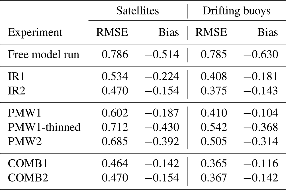
The RMSE is higher in PMW1 than in IR2 when validating against SSTs from satellites and when validating against SSTs from drifting buoys. However, the bias of PMW1 is smaller than the bias of IR2 when validating against SSTs from drifting buoys, indicating that PMW SSTs are valuable to assimilate to reduce the model's systematic error. When validating against IR SSTs, PMW1 has a larger bias than IR2. Upon inspection of the spatial distribution of the model minus observation differences that contribute to this elevated bias value, it is clear that the elevated bias is mainly caused by elevated errors in regions where the coastal current extends into the parts of the model domain that are considered in the validation. Thus, this larger bias does not reflect the ability of the PMW SST data to adjust the model. Rather, the elevated bias values are caused by advection of cold coastal water, which is unconstrained by PMW SSTs, into the region used for calculating the validation statistics.

When applying the supermod operator to assimilate the PMW SSTs, both RMSEs and biases are increased in comparison with PMW1. PMW2 does, however, validate better than both the free model run and the PMW1-thinned experiment. Compared with PMW1, we find that the increments in PMW2 are relatively weak. The mean increment of PMW1 and PMW2 during the first assimilation window, where the experiments share the same initial conditions, demonstrate this increment difference: the mean increment in PMW1 is ∼ 0.39 ^∘C (increment standard deviation: ∼ 0.49 ^∘C), whereas PMW2 has a mean increment of ∼ 0.04 ^∘C (increment standard deviation: ∼ 0.06 ^∘C). That the increments are reduced in PMW2 is in accordance with how the supermod operator works. As demonstrated in Fig. 6, the amplitude of the increment decreases with increasing footprint size when the observation error remains unchanged.

The difference between the SST increment amplitudes in PMW1 and PMW2 is, in addition, visually illustrated in Fig. 7a and b. Even though the number of observations in PMW2 is significantly reduced compared to PMW1 due to thinning, the supermod operator is able to spread the impact of the observations over the footprint area, yielding an increment pattern that overall resembles the pattern seen in PMW1. Both PMW1 and PMW2 are cooled in the North Sea in the southern part of the domain, while the larger part of the domain is heated. Also, a large positive whirl in the increments can be seen just north of 69^∘ N in both panels. The most notable difference between the experiments is that the increments are weaker and more smooth in PMW2, which is what we would expect, as the supermod operator is designed to adjust the average SST in an area corresponding to the footprint of the observations. Note that the high level of detail in the increments in PMW1 does not necessarily lead to a more detailed SST field in the analysis state. In many cases, detailed increments reflect that structures present in the background state have been strongly modified or even removed. Other notable differences between the experiments are the areas of strong, positive increments in PMW1 (north of 72^∘ N, close to the western boundary at 66^∘ N, and close to the coast around 63^∘ N), which are not subject to enhanced heating in PMW2, as well as some cold patches in PMW1 that are not seen in PMW2. Furthermore, to separate the effect of the supermod operator and the observation thinning, we study the results from PMW1-thinned, in which a thinned set of PMW SSTs is assimilated without applying the supermod operator. We find that only a thinning of the observations is not sufficient to spread the increments over the observation footprint (Fig. 7c). The thinning itself does not handle the spatial resolution mismatch between the PMW SSTs and the model, and the supermod operator is required to spread the information from each observation over an area of similar size to the observation footprint. Calculated error statistics also show that PMW1-thinned validates worse than PMW1 and PMW2 when validating against SSTs from satellites and when validating against SSTs from drifting buoys (Table 3). This indicates that the information provided by the thinned set of PMW SST observations is used more efficiently when the observations are assimilated with the footprint operator activated.

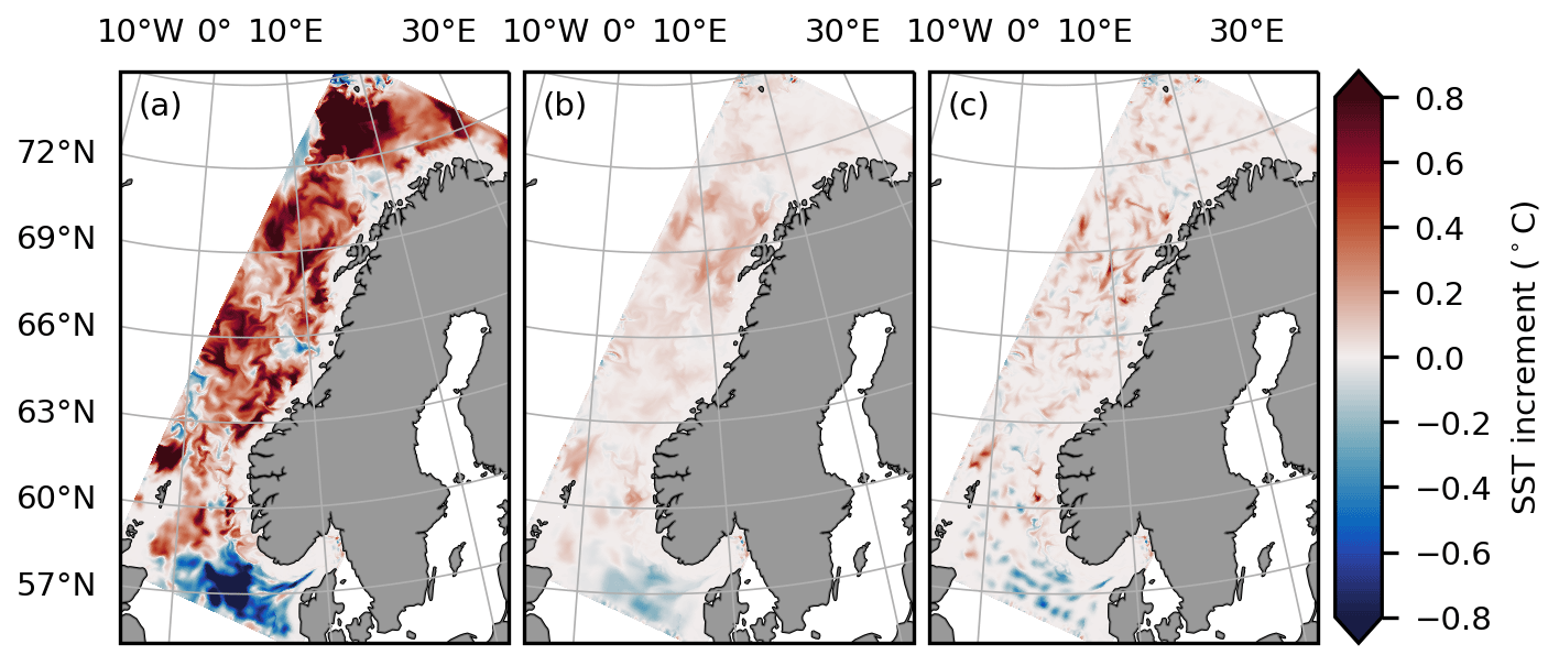
Figure 7 SST increments at the last time step in the first assimilation window. Increments of experiments (a) PMW1, (b) PMW2, and (c) PMW1-thinned.

When validating against satellite SSTs, the performance of COMB1 is found to be superior to that of IR2, while COMB2 is found to produce results that are identical to those of IR2. For the validation against SSTs from drifting buoys, both COMB1 and COMB2 perform better than IR2. These results imply that the PMW SST data set provides the model with information not seen by the IR SSTs and that the supermod operator is able to pass along this information to some extent. We also find that COMB1 validates better than COMB2. This can partly be explained by the differences between the magnitudes of the increments resulting from assimilating the PMW SST observations, as discussed when comparing PMW1 and PMW2. To verify that the addition of PMW SSTs to the assimilated data set indeed has a positive impact with regards to the validation against SSTs from drifting buoys, we tested for statistical significance as follows. For each of the experiments IR2, COMB1, and COMB2, every individual SST difference (model minus observation) was randomly assigned to 1 of 22 subsets. RMSE and bias were calculated for these unique subsets, and a Wilcoxon signed-rank test was used to test these RMSEs and biases for statistical significance. The tests showed that the differences between the RMSEs in COMB1, COMB2, and IR2 are statistically significant at the 99 % confidence level. The same applies to the better bias in COMB1 compared to the bias in IR2. There is, however, no significant difference between the biases calculated from COMB2 and IR2.

To investigate whether the improved error statistics of COMB1 and COMB2 can be explained by the extra information PMW SSTs provide to the model when IR SSTs are unavailable, error statistics are now calculated separately for cloudy and clear-sky conditions. The validation of SST during cloudy conditions is calculated using only reference satellite SSTs within regions where IR SSTs were unavailable during the previous analysis cycle. Similarly, only reference satellite SSTs in regions where there were clear skies in the same analyses are used for validation of clear-sky conditions. As we use the background model states for validation purposes, regions that experienced heavy cloud cover and thus poor coverage of IR SSTs during the previous assimilation cycle are not necessarily poorly sampled by IR SST during the period used for validation. The resulting error statistics are shown in Table 4. We find that both COMB1 and COMB2 perform better than IR2 during cloudy conditions, both in terms of RMSE and bias. Using the same method as before to calculate the statistical significance, we find that the lower RMSE and bias in COMB1 and COMB2 compared to IR2 are statistically significant. There is, however, no significant improvement in COMB2 over IR2 during clear-sky conditions. The improvement seen in COMB1 is also more pronounced during cloudy conditions than during periods with good IR SST coverage, which indicates that PMW SSTs indeed provide valuable extra information in the absence of IR SSTs.

Table 4 SST RMSE (^∘C) and bias (^∘C) calculated using satellite SSTs as reference. Validation performed during cloudy (left column) and clear-sky conditions (right column). The number of reference observations is ∼ 1.7 × 10⁶ (cloudy) and ∼ 3.5 × 10⁷ (clear-sky).

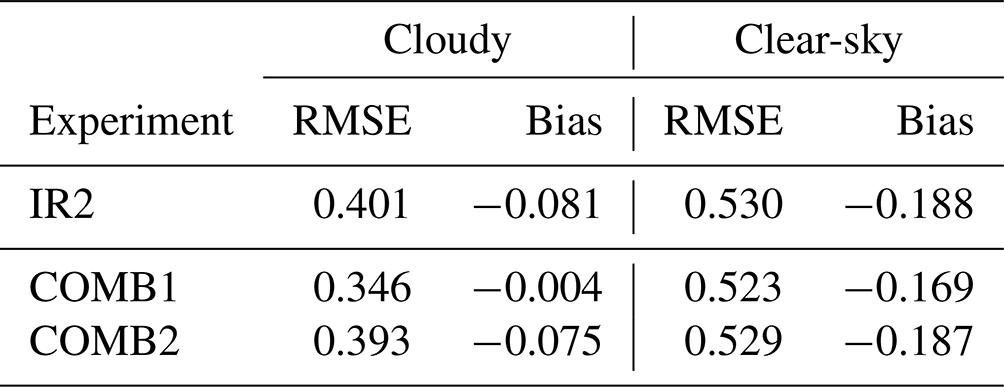
Figure 8 illustrates how PMW observations compensate for IR SST data deficiency. SSTs assimilated in IR2 during the assimilation cycle covering 8–10 June 2018 are shown in Fig. 8a, while the SST increments at the last time step of this cycle are shown in Fig. 8b. Figure 8e shows the increments inside the black box in Fig. 8b. The presence of clouds limits the IR SST coverage, particularly in the southwestern part of the domain. A cluster of IR SST observations around the Shetland Islands causes a cooling of the model. However, the general lack of observations in this region leaves behind a larger area with no adjustments to the SST field. For COMB2, the assimilated observations and the increments are shown in Fig. 8c and d, respectively. The increments inside the black box in Fig. 8d are shown in Fig. 8f. Notice that the regions without IR SST observations in Fig. 8a are now covered by PMW SSTs. The addition of this information to the model causes the SST field to adjust, such that a larger area is cooled.

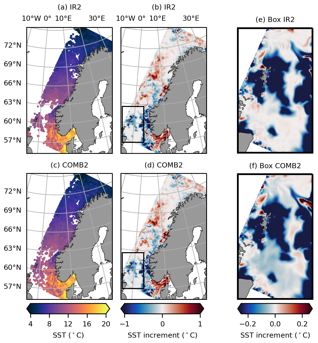
Figure 8 SST observations assimilated in (a) IR2 and (c) COMB2 during the assimilation cycle covering 8–10 June 2018, and SST increments in (b) IR2 and (d) COMB2 at the last time step of this assimilation cycle. A zoom-in of the increments inside the black box in (b) and (d) is shown in (e) and (f), respectively. Note the change in the scale of the color bar.

4.3 SST power spectra

Spectral analysis is a technique that can be used to decompose the information contained in an observed or modeled field into different spatial scales. Specifically, spectra can be computed for modeled or observed SST fields to evaluate the spatial resolution of the SST structures contained within the field (e.g., Reynolds and Chelton, 2010; Brasnett and Colan, 2016; Castro et al., 2017; Pearson et al., 2019; Schubert et al., 2019; Janeković et al., 2022). The reason for this is that a spectrum holds information about the SST variability at different spatial scales. Hence, a reduction in the spectral density at shorter wavelengths reflects that SST structures at these scales have been dampened, i.e., that the field has become more smooth.

SST data are often decomposed into spectral space using the discrete Fourier transform (DFT), a transformation that requires the data to be periodic. Periodicity can be retained by spatially detrending the data or by windowing, i.e., multiplying the field by a function such that the interior of the domain retains its structures while the boundaries drop off and approach zero. As noted by Denis et al. (2002), a disadvantage of detrending and windowing is that these methods modify the resulting spectrum by removing important information in the original data. To avoid these problems, they propose an alternative to the DFT, namely the discrete cosine transform (DCT). We have chosen to use this method for the spectral analysis performed in this study. When applying the DCT, the input fields are made periodic in space by mirroring the fields prior to the transformation. The reader is referred to Denis et al. (2002) for a thorough description of the DCT.

For each time step of the background, we apply the DCT to the two-dimensional SST field inside the dashed box shown in Fig. 2. This transformation into spectral space, as well as the subsequent calculation of the two-dimensional spectral variance array, follows the methodology described in Denis et al. (2002). The spectral variance array consists of elements, σ²(m,n), where m and n are the adimensional wavenumber axes (i.e., the grid cell indexes in both horizontal directions), and each of these variance elements is associated with a normalized radial wavenumber,

$$\begin{array}{}\text{(3)}& \mathit{\kappa }=\sqrt{{\displaystyle \frac{m^{\mathrm{2}}}{N_i^{\mathrm{2}}}}+{\displaystyle \frac{n^{\mathrm{2}}}{N_j^{\mathrm{2}}}}},\end{array}$$

where N_i and N_j are the domain's total number of grid cells in each horizontal direction. The radial wavenumbers are adimensional, but they can be converted into wavelengths through the following equation:

$$\begin{array}{}\text{(4)}& \mathit{\lambda }={\displaystyle \frac{\mathrm{2}\mathrm{\Delta }}{\mathit{\kappa }}},\end{array}$$

where Δ is the grid cell spacing. To create a one-dimensional SST power spectrum, all individual spectral variance elements, σ²(m,n), that fall within a given wavelength bin, λ, are summed in order to find the total variance in this bin. As described in Denis et al. (2002), the variance elements that contribute to wavelength bin λ are those variances that fall within the wavelength band bounded by λ and λ+Δλ. However, we have modified this approach according to Ricard et al. (2013), such that the variances within a wavelength band are proportionally distributed between the two bounding wavelength bins based on the variances' proximity to the bins. The one-dimensional SST power spectra calculated for each time step are subsequently averaged in time to provide a mean SST power spectrum. Notice that, while the mean SST power spectra are functions of the adimensional wavenumber, we will refer to the wavelength calculated from Eq. (4) when we present the results.

Figure 9 shows the mean SST power spectra calculated for each experiment (except IR1 and PMW1-thinned). For wavelengths smaller than ∼ 120 km, we find that the spectrum from PMW1 has significantly lower power than both the spectrum calculated from IR2 and that of the free model run (not shown). Assimilating PMW SSTs without using the supermod operator thus has a smoothing effect on the modeled SST, indicating that the average effect of the high level of detail seen in the increments (Fig. 7) is a removal or smoothing of structures present in the background state. This smoothing effect is also present in the spectrum calculated from COMB1, where IR SSTs are added to the assimilated data set: the spectrum from COMB1 follows that of PMW1 at most wavelengths and is more or less similar to PMW1's spectrum at wavelengths in the range of ∼ 35–120 km. This result is within expectations, as PMW SSTs represent a mean value over a large footprint of the actual SST field. With a traditional observation operator, this mean value is compared to individual model grid points, and any small-scale deviation from this mean value in the model is thus damped in the analysis.

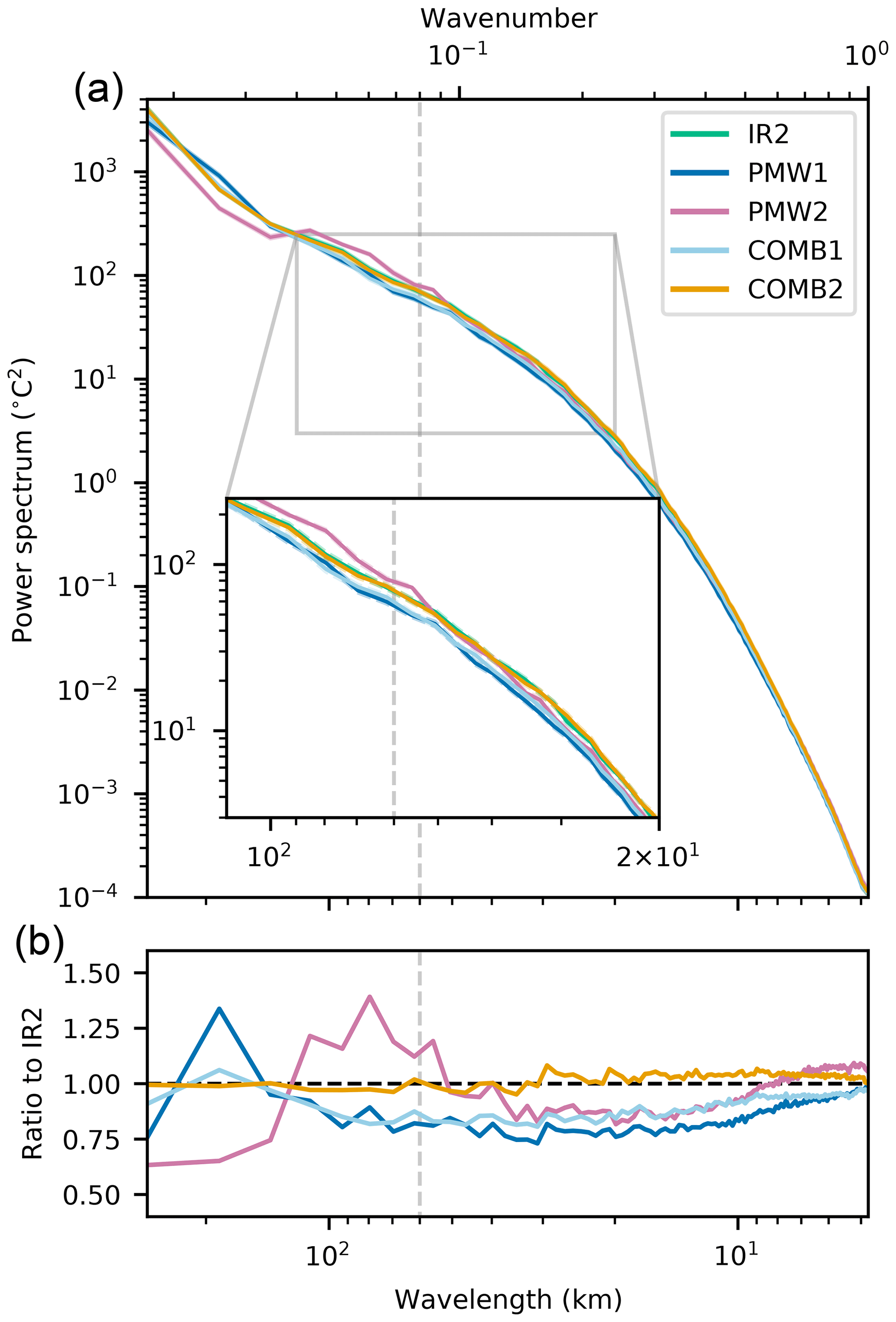
Figure 9 Upper panel shows SST power spectra with wavelengths ranging from 278.4 km (length of the shortest edge of the domain used to calculate spectra) to 4.8 km (double the grid spacing). Shading is applied to indicate the 95 % confidence interval on the mean spectrum, and this is calculated using the jackknife method. Notice that the shading is hard to detect due to the narrowness of the confidence interval. Inset zoom shows the spectra at wavelengths ranging from 120 to 20 km. The lower panel shows the ratio of the experiments' spectra to the spectrum from IR2. A dashed gray line is drawn at 60 km, which is approximately the size of the major axis of the elliptic PMW SST footprint.

The spectrum from PMW2 has more power than that from PMW1 at all scales smaller than ∼ 120 km, which means that PMW2 resolves more SST structures at these scales. The peak in the ratio between PMW2 and IR2, which is found at ∼ 80 km, is also present in the ratio between the free model run and IR2 (not shown). In fact, we find that the spectrum of PMW2 follows the spectrum of the free model run at most spatial scales but with less power at all spatial scales. Furthermore, we see in Fig. 9 that the power spectrum from COMB2 is more or less identical to that of IR2 at all spatial scales. Even with lower observation errors for the PMW SSTs (decreasing the α) and thus stronger increments, COMB2 stays similar to IR2, with ∼ 1 as the ratio between COMB2's and IR2's spectrum at all spatial scales (not shown). These findings suggest that using the supermod operator prevents smoothing of small-scale structures present in the field: as PMW SSTs are now compared to mean model values, they do not penalize variations of the SST at spatial scales they do not resolve.

SST power spectra are also calculated for each experiment using the last day of the analyses from each analysis cycle. These spectra were compared with the corresponding background spectra to examine if the assimilation changes the spatial scales of the background SST structures within each experiment. Figure 10 shows the ratio of the analysis spectrum to the background spectrum for each experiment. We find that the analyses in PMW1 experience a loss of SST structures with spatial scales of ∼ 20–80 km and that the analyses in COMB1 have fewer SST structures at scales of ∼ 40–60 km. The other experiments' analyses do not experience a significant loss due to the assimilation of the observations.

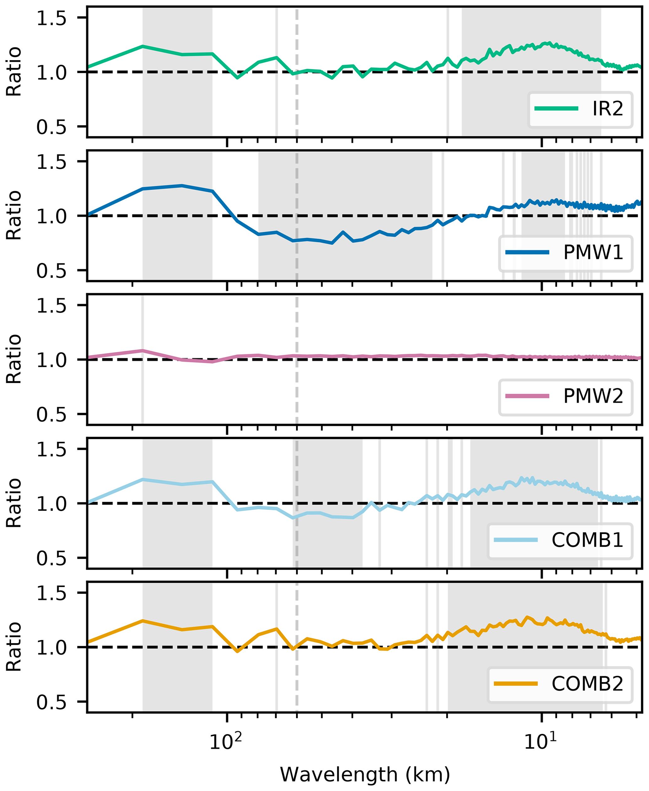
Figure 10 Ratio of the analysis spectrum to the background spectrum for each experiment. Gray shading is applied at wavelengths where there is no overlap of the 95 % confidence intervals of the mean analysis spectrum and the mean background spectrum. Dashed gray line drawn at 60 km.

5 Discussion

Our results suggest that it is beneficial to assimilate the PMW SSTs in conjunction with the IR SSTs in order to reduce the errors in modeled SST. This is verified by comparing the error statistics of COMB1 and COMB2 to IR2. The comparison of error statistics during clear-sky and cloudy conditions suggests that the reduced errors in COMB1 and COMB2 largely originate from the additional information given to the model during cloudy conditions when there is a shortage of IR SSTs. Figure 8, which shows the SST increments in such cloudy regions, demonstrates the supermod operator's ability to pass along the relevant information seen by the PMW SSTs. Here, the assimilated PMW SST observations cool the model SST in a region of sparse IR SST coverage. The few available IR SSTs in that region confirm this cooling. However, these IR SSTs are not sufficient to correct the SST of the whole region when assimilated on their own.

While error statistics show that COMB1 validates better than COMB2, we find that COMB1 yields smoother SST fields than what is found in IR2. This indicates that neglecting to account for the mismatch in spatial scales when assimilating PMW SSTs may be disadvantageous. The smoothing of COMB1 is demonstrated by the calculated SST power spectra. We find that both PMW1 and COMB1 return smoother SST fields than IR2 at spatial scales smaller than ∼ 120 km. This upper limit is approximately twice the size of the major axis of the elliptic PMW SST footprint. Thus, the limit corresponds to the expected effective resolution of the SST structures resolved by the PMW SST observations. It is striking that the affected spatial scales in PMW1 and COMB1 correspond to scales smaller than or similar to this effective resolution. Furthermore, the fact that additional information from the IR SSTs in COMB1 does not prevent smoothing indicates that the PMW SSTs have a substantial impact on the final product. However, assimilating the PMW SSTs through the supermod operator, which was performed in COMB2, does not result in a smoothing of the SST structures. This demonstrates that the operator is a good alternative approach to assimilating observations of coarser spatial resolution than the model.

As demonstrated in Sect. 3.1, the amplitude of the increments decreases with increasing footprint size when the supermod operator is applied if the observation errors are kept unchanged. A suitable choice for the observation error covariance is important for the overall performance of all assimilation algorithms. To assess the observation errors prescribed to the different products assimilated in this study, we have applied the diagnosis proposed by Desroziers et al. (2005). The results indicate that the chosen observation errors are too high for all assimilated products. For PMW SSTs, we see the same tendency of overestimation both with and without the supermod operator activated. By setting α=0.8 to reduce the observation errors, we obtain improved error statistics for PMW2 without any indication of overfitting to the observations, whereas the results for PMW1 barely change (not shown). However, for PMW1, this lower error introduces artifacts in the modeled SST fields. These artifacts are similar to those that can be seen in the PMW observations, which may be caused by the large footprint size and by the regridding and interpolation during the processing. Due to this degradation of PMW1, and to be able to fairly assess all experiments, the observational error was constructed using the higher α=2 for all experiments shown in this study. Moreover, the assimilation of PMW SSTs using the supermod operator could potentially be improved by optimization of the prescribed footprint size. If a smaller footprint could be applied without smoothing the modeled SST, this could both yield larger increments and increase the number of observations available for assimilation. Furthermore, the effect of a less strict thinning of observations could be explored.

Finally, all of the experiments were during local spring, which is a period when the modeled SST undergoes great changes. Such changes make it challenging to sustain highly skilled forecasts, and we chose this period due to these challenges. However, the chosen period is not heavily affected by clouds. The impact of assimilating PMW SSTs is possibly greater during winter when the oceanic regions along the Norwegian coastline experience high cloud coverage.

6 Conclusions

Correcting satellite SSTs for biases through the implemented bias correction scheme improves the modeled SST. The bias correction scheme is easy to implement and apply, since it is separate from the data assimilation process.

While assimilating IR SSTs reduces the modeled SST errors, an additional reduction is achieved if PMW SSTs are assimilated in conjunction with the IR SSTs. This error reduction is mainly caused by the information the PMW SSTs provide in cloudy regions. However, if we assimilate the PMW SSTs without considering their large footprint sizes, we end up smoothing the modeled SST structures of spatial scales smaller than twice the PMW SST footprint. By introducing the supermod operator, we have shown that the PMW SST observations can be assimilated into the ocean model without causing any spatial smoothing of the modeled SST. Our supermod operator is easy to implement and can be used to assimilate other observation variables that have a coarser spatial resolution than the resolution of the model.