Joint observation–model mixed-layer heat and salt budgets in the eastern tropical Atlantic

In this study, we use a joint observation–model approach to investigate the mixed-layer heat and salt annual mean as well as seasonal budgets in the eastern tropical Atlantic. The regional PREFCLIM (PREFACE Climatology) observational climatology provides the budget terms with a relatively low spatial and temporal resolution compared to the online NEMO (Nucleus for European Modeling of the Ocean; Madec, G., 2014) model, and this is later resampled as in PREFCLIM climatology. In addition, advection terms are recomputed offline from the model as PREFCLIM gridded advection computation. In the Senegal, Angola, and Benguela regions, the seasonal cycle of mixed-layer temperature is mainly governed by surface heat fluxes; however, it is essentially driven by vertical heat diffusion in the equatorial region. The seasonal cycle of mixed-layer salinity is largely controlled by freshwater flux in the Senegal and Benguela regions; however, it follows the variability of zonal and meridional salt advection in the equatorial and Angola regions, respectively. Our results show that the time-averaged spatial distribution of NEMO offline heat and salt advection terms compares much better to PREFCLIM horizontal advection terms than the online heat and salt advection terms. However, the seasonal cycle of horizontal advection in selected regions shows that NEMO offline terms do not always compare well with PREFCLIM, sometimes less than online terms. Despite this difference, these results suggest the important role of small-scale variability in mixed-layer heat and salt budgets.

1 Introduction

The interaction between ocean and atmosphere plays a crucial role in the climate system. This interaction involves heat and freshwater fluxes, which affect temperature and salinity variations in the upper-oceanic mixed layer. Therefore, sea surface temperature and salinity (SST, SSS) are two key climate variables, and understanding the balance of processes determining their variability is a key requirement to accurately simulating the climate system.

In the eastern tropical Atlantic, seasonal climate variability is mostly associated with the West African monsoon (WAM) and strongly linked with SST and SSS variations. SST is characterized here by a strong seasonal cycle, which influences the regional climate, particularly the large-scale atmospheric circulation and rainfall over the ocean and African continent (Carton and Zhou, 1997; Foltz et al., 2013; Kushnir et al., 2006). In the Gulf of Guinea, the seasonal formation of the Atlantic cold tongue (ACT), associated with equatorial upwelling, is the main feature associated with SST seasonal variations (Chang et al., 2006; Peter et al., 2006; Caniaux et al., 2011). This seasonal cooling creates an intense meridional SST front that enhances southern trade winds and shifts the Intertropical Convergence Zone (ITCZ) northward, which triggers the WAM (Philander and Pacanowski, 1981; Picaut, 1983; Waliser and Gautier, 1993; Caniaux et al., 2011). In the Angola–Benguela frontal zone off southwestern Africa, SST variability also has an impact on coastal precipitation (Reason and Rouault, 2006). Conversely, the atmospheric conditions in the eastern tropical Atlantic impact SST, as trade winds are the main driver of eastern boundary upwelling systems found along the coasts of Angola–Namibia and Senegal–Mauritania.

Like SST, SSS is an essential climate variable. Its variations are closely linked to the global hydrological cycle, as freshwater exchanges between the ocean and atmosphere control its mean large-scale distribution (Durack and Wijffels, 2010; Bingham et al., 2012): regions of high SSS are dominated by evaporation, while regions of low SSS are dominated by precipitation. In the eastern tropical Atlantic, the intense precipitation under the ITCZ has a strong impact on seasonal variability of SSS. For example, off Senegal and Guinea, SSS decreases in boreal fall following the period when the ITCZ reaches its most northern position, which leads to a maximum in precipitation and runoff from Senegal and Gambia rivers (Camara et al., 2015). The eastern tropical Atlantic is indeed characterized by low SSS plumes due to strong river discharges, including the Congo River (the second-largest outflow in the world after the Amazon River) and the Niger River in the Gulf of Guinea. SSS variations are also associated with upwelling. In the equatorial Atlantic, SSS increases during the development of the Atlantic cold tongue (ACT) in boreal spring–summer (Schlundt et al., 2014; Da-Allada et al., 2014). Summer upwelling at the northern coast of the Gulf of Guinea also increases coastal SSS (Alory et al., 2021). Off Angola, relatively high SSS is observed during the upwelling season in August, while low SSS appears in March and October–November (Kopte et al., 2017; Awo et al., 2022). In the Benguela upwelling system further south, the maximum in SSS appears in April and the minimum in October (Junker et al., 2017).

SST and SSS have already been the focus of several studies in the eastern tropical Atlantic. Studies only based on observations (in situ and/or satellite), and others combining observational data and model data, show a variety of physical processes contributing to the heat and salt budget with a different balance from one region to another (Foltz et al., 2003; Foltz and McPhaden, 2008; Da-Allada et al., 2013, 2014).

In the northern tropical Atlantic far from the coast, the heat budget is largely driven by surface heat fluxes, essentially solar radiation varying with the cloudy ITCZ position (Carton and Zhou, 1997). Off northwestern Africa in the Senegal region, the seasonal cycle of SST is associated with coastal upwelling modulated by the seasonal variations of alongshore winds. In the equatorial zone, the mixed-layer heat budget is mainly controlled by surface heat fluxes, of which mainly the solar radiation is important (Carton and Zhou, 1997; Foltz et al., 2003; Yu et al., 2006). The dominance of the surface heat flux is highlighted by a recent study based on PIRATA buoy data off the Equator, in particular at the 6^∘ S, 8^∘ E position. At this latitude, seasonal variations in SST governed by solar flux and latent heat flux are shown to be associated with the meridional migration of the ITCZ and the formation of low-level marine stratocumulus (Scannell and McPhaden, 2018). However, other oceanic processes can also play an important role in the seasonal heat budget. These include zonal advection and vertical mixing, which are important during the formation of the ACT (Foltz et al., 2003; Hummels et al., 2014; Schlundt et al., 2014). However, the influence of vertical mixing in the heat budget remains low in the eastern (from 0^∘ E to the coast of Africa) compared to the central equatorial Atlantic (Jouanno et al., 2011; Hummels et al., 2013). This is explained by the strong stratification in the eastern equatorial Atlantic due to the transport of low-salinity and warm waters from the Gulf of Guinea, which contributes to reducing the vertical mixing. The low salinity is associated with the intense precipitation and important freshwater intakes from the Niger and Congo rivers in the Gulf of Guinea. Off Angola, annual variability of SST is driven by meridional wind stress, causing coastal upwelling, and thermocline depth variations forced by remote equatorial effects (Carton and Zhou, 1997).

In the northeastern tropical Atlantic, including in the Senegal region, the salt budget is controlled by freshwater fluxes. The net mixed-layer salinity variations are, however, weak because of the compensation between the atmospheric and oceanic terms (Camara et al., 2015). In the eastern equatorial Atlantic and Gulf of Guinea, horizontal advection and vertical mixing play a dominant role in determining the seasonal cycle of salt budget, which cannot be explained by freshwater fluxes only (Tzortzi et al., 2013; Da-Allada et al., 2013, 2014). This dominance of zonal advection and vertical processes extends southward and in the Angola coastal region (Camara et al., 2015).

In addition, it can be noted that various approaches have been used to estimate the heat and salt budgets in the tropical Atlantic, in particular the advection terms. Foltz et al. (2003) analyzed the mixed-layer heat balance at PIRATA mooring locations, where they computed the heat advection from monthly gridded climatologies of near-surface horizontal velocity, based on ship drifts and Lagrangian drifters, and SST gradient fields based on a combination of ship, buoy, and satellite data. Wade et al. (2011) used a similar SST product but satellite-derived currents to estimate the heat advection every 10 d at positions of Argo profiles. Then monthly averages in nine boxes covering the Gulf of Guinea were used to study the seasonal cycle of mixed-layer heat as observed by Argo. Da-Allada et al. (2013) developed an original mixed-layer model of the tropical Atlantic at monthly, 1^∘ resolution, with salinity driven by observation-based climatological freshwater budget terms, and several in situ and satellite surface currents products were tested for advection to identify processes driving SSS seasonal variations. With the same objective, Da-Allada et al. (2014) and Camara et al. (2015) used slightly different tropical Atlantic configurations of the NEMO (Nucleus for European Modeling of the Ocean; Madec, G., 2014) OGCM (ocean general circulation model), with mixed-layer salinity budget terms computed online, on the model spatial grid (0.25^∘), and at each time step (20 min). We know from analyzing online diagnostics that the nonlinear advective terms cannot be neglected. Observational data, however, often have lower temporal and/or spatial resolution than would be necessary to fully capture the nonlinear terms. Moreover, it is much more difficult to estimate subsurface vertical terms than surface terms with observations; this leads to a non-negligible residual term, which interpretation is problematic. Online computation in an OGCM is practically the only way to close a mixed-layer heat and salt budget.

Nonlinear terms are associated with turbulence. In eddy-resolving models, they represent mesoscale activity related to eddies and tropical instability waves (TIWs). The characteristic size of eddies is given by the Rossby radius, which increases equatorward and has a minimum value of 30–40 km in the 30^∘ S–30^∘ N subtropical band (Chelton et al., 1998). TIWs have been shown to play an important role in the heat budget in the central equatorial Atlantic (Foltz et al., 2003; Grodsky et al., 2005; Jochum et al., 2005; Peter et al., 2006; Lee et al., 2014; Heukamp et al., 2022; Tuchen et al., 2022). In the tropical Atlantic, eddies have been detected mostly in coastal upwelling systems, where they are likely to affect mixed-layer heat and salt budgets too (Djakouré et al., 2014; Aguedjou et al., 2019).

In this paper, we exploit for the first time a recently produced tropical Atlantic mixed-layer heat and salt budget observation-based climatology. Moreover, we use a joint observation–model approach that has rarely been used: we compare the mixed-layer heat and salt budget terms estimated from observations to those simulated by a high-resolution OGCM simulation in the eastern tropical Atlantic. A sensitivity test to the spatiotemporal resolution at which advection terms are computed in the model is conducted. This comparison should allow providing a high-level model validation, isolating the contribution of mesoscale advection in the mixed-layer budgets, and quantifying the uncertainty in the different budget terms. We particularly focus for the mixed-layer budgets on the upwelling regions where oceanic processes are expected to be dominant. The observational product, the model, and the methodology used are presented in Sect. 2. Section 3 contains the results of observation–model comparison regarding mean heat and salt budgets, as well as their seasonal variability in selected regions. In Sect. 4, a discussion and conclusion are presented.

2 Data and methods

2.1 Data

2.1.1 Observations

We use the PREFCLIM (PREFACE Climatology) observed seasonal climatology of mixed-layer heat and salt budgets covering the eastern tropical Atlantic (Rath et al., 2016). It has been produced in the framework of the European PREFACE (Enhancing prediction of tropical Atlantic climate and its impacts) project, which aimed at improving climate models in the tropical Atlantic. This monthly climatology is derived from all hydrographic data publicly available covering the region, including Argo float data (Argo, 2000) and glider measurements conducted by GEOMAR between 2002 and 2015 (for more details, see https://gliderweb.geomar.de, last access: 27 April 2023), also completed by data from hydrographic stations in Senegal, Angola, and Namibia waters collected during cruises of the EAF-Nansen. In addition, this climatology uses data from other projects of PREFACE partners like PIRATA (Prediction and Research Moored Array in the Tropical Atlantic, Bourlès et al., 2019).

These data have been gridded using an interpolation scheme including isobath-following and front-sharpening components (Schmidtko et al., 2013). Mixed-layer properties like temperature, salinity, and depth are provided with a spatial resolution of $\mathrm{0.25}{}^{\circ }\times \mathrm{0.25}{}^{\circ }$, while mixed-layer budget terms and horizontal velocities used to compute advection terms are given with a lower spatial resolution of $\mathrm{0.25}{}^{\circ }\times \mathrm{0.25}{}^{\circ }$. The mixed-layer depth (MLD) is computed following the Holte and Talley (2009) method. For individual ocean profiles, this hybrid method models the general shape of each profile, searches for physical features in the profile, and calculates the MLD by using threshold and gradient methods to form a suite of possible MLD values. Then it analyzes the patterns associated with this formed suite in order to select a final MLD estimate. Surface heat fluxes are derived from the TropFlux data set (Kumar et al., 2012), the freshwater flux associated with evaporation is computed from latent heat flux of TropFlux, and precipitation is derived from GPCP (Global Precipitation Climatology Project) version 2.2 (Huffman et al., 2009). Heat and salt horizontal advection terms (split into zonal and meridional components) have been calculated using the near-surface gridded velocity field based on the measurements of surface drifters (Lumpkin et al., 2013) and Argo floats from the YOMAHA data set (Lebedev et al., 2007), which is combined with a gridded temperature and salinity gradient field. These will be called the gridded advection terms. This climatology was supplemented with an additional product of heat and salt advection using estimated velocities from each of the drifter and float data points used for the gridded velocity fields combined with the full high-resolution hydrographic climatology. These alternative terms of heat and salt advection will be called Lagrangian advection terms here and denoted by Obs-drift to highlight the difference from the previous terms. The full description of this climatology is presented in a PREFACE project deliverable (Dengler and Rath, 2015).

2.1.2 Model

We use a regional configuration of the NEMO (Nucleus for European Modeling of the Ocean; Madec, G., 2014) oceanic model version 3.6. This regional simulation covers the tropical Atlantic (35^∘ S^∘–35^∘ N, 100^∘ W–15^∘ E). It uses a horizontal Arakawa grid of type C, with a 0.25^∘ horizontal resolution. The vertical grid, in z coordinates, has 75 levels, including 12 levels within the upper 20 and 24 m in the upper 100 m of the ocean. The model is forced by daily outputs of the global MERCATOR reanalysis GLORYS2V3 at lateral boundaries. Atmospheric fluxes of heat, fresh water, and momentum used for surface forcing are from the DRAKKAR Forcing Set version 5.2 (DFS5.2) product (Dussin et al., 2016). The surface fluxes are prescribed following a bulk formula (Large and Yeager, 2009). River runoff is introduced as surface fresh water at river mouths and is based on a monthly climatology (Dai and Trenberth, 2002). Heat and salt budget terms are computed online, at each model time step (20 min), and vertically integrated in the mixed layer. The mixed-layer depth is computed following a density criterion: a 0.03 kg m⁻³ difference relative to the density at 10 m (de Boyer Montégut et al., 2004). The description of this model is more detailed in Hernandez et al. (2016). In this paper, we use climatological monthly averages of mixed-layer properties averaged for the 1980–2015 period to compare with similar terms available from observations. This climatological approach is used in many studies on the mixed-layer budget (Da-Allada et al., 2014; Camara et al., 2015). This NEMO regional configuration has already been used to study the Gulf of Guinea salinity distribution and variability at seasonal and interannual timescales (Da-Allada et al., 2017; Awo et al., 2018).

2.2 Methods

In this paper, the driving processes of the seasonal variability of mixed-layer temperature and salinity in selected regions are quantified through heat and salt budgets from the NEMO model. This approach has been already used in several studies based on observations and models (Da-Allada et al., 2013; Hasson et al., 2013). In the following, as mixed-layer temperature and salinity are very close to SST and SSS, respectively, we indifferently use the vocabulary. The heat budget evolution and salt budget evolution within the mixed layer are respectively given by Eqs. (1) and (2), already used in previous studies (Peter et al., 2006; Jouanno et al., 2011; Da-Allada et al., 2014; Schlundt et al., 2014):

$$\begin{array}{}\text{(1)}& {\displaystyle }\begin{array}{rl}{\displaystyle \frac{\partial \text{SST}}{\partial t}}=& \underset{A}{\underbrace{{\displaystyle \frac{(Q^{\ast }+Q_{\text{s}}(\mathrm{1}-f_{z=-h})}{{\mathit{\rho }}_{\mathrm{0}}{c}_{\text{p}}h}}}}\\ & \underset{B}{\underbrace{-\langle U\cdot {\partial }_{X}T\rangle -\langle V\cdot {\partial }_{Y}T\rangle }}\underset{C}{\underbrace{+D_l\left(T\right)}}\\ & \underset{D}{\underbrace{-\langle W\cdot {\partial }_{Z}T\rangle -{\displaystyle \frac{(k_Z{\partial }_{Z}T{)}_{z=-h}}{h}}-{\displaystyle \frac{\mathrm{1}}{h}}{\displaystyle \frac{\partial h}{\partial t}}(\text{SST}-T_{z=-h})}},\end{array}\text{(2)}& {\displaystyle }\begin{array}{rl}{\displaystyle \frac{\partial \text{SSS}}{\partial t}}=& \underset{A}{\underbrace{{\displaystyle \frac{(E-P)\text{SSS}}{h}}}}\\ & \underset{B}{\underbrace{-\langle U\cdot {\partial }_{X}S\rangle -\langle V\cdot {\partial }_{Y}S\rangle }}\underset{C}{\underbrace{+D_l\left(S\right)}}\\ & \underset{D}{\underbrace{-\langle W\cdot {\partial }_{Z}S\rangle -{\displaystyle \frac{(k_Z{\partial }_{Z}S{)}_{z=-h}}{h}}-{\displaystyle \frac{\mathrm{1}}{h}}{\displaystyle \frac{\partial h}{\partial t}}(\text{SSS}-S_{z=-h})}}\\ & +\underset{A^{\prime }}{\underbrace{{\displaystyle \frac{-R\cdot \text{SSS}}{h}}}},\end{array}\end{array}$$

where T is temperature, S is salinity, and h is the mixed-layer depth; U, V, and W are the zonal, meridional, and vertical components of the velocity vector; and D_l(.) is lateral diffusion. In Eq. (1), Q^∗ and Q_s represent the non-solar and solar components of surface heat flux, respectively, and $f_{z=-h}$ represents the fraction of shortwave radiation reaching depths below the base of the mixed layer (and hence not available for heating up the mixed layer itself).

The left-hand side of Eq. (1) represents the mixed-layer temperature tendency term, and the right-hand side represents all terms contributing to the heat budget. Namely, term A is the surface heat flux decomposed (from left to right) into non-solar flux (longwave, latent heat, sensible heat) and solar flux (shortwave). Term B is horizontal temperature advection, decomposed into zonal and meridional components, term C is lateral temperature diffusion, and term D represents vertical oceanic processes. D contains (from left to right) vertical temperature advection, vertical temperature diffusion at the base of the mixed layer, and entrainment that represents mixed-layer temperature variations due to changes in the mixed-layer depth.

The left-hand side of Eq. (2) represents the mixed-layer salinity tendency term, and the right-hand side represents all terms contributing to the salt budget. Namely, term A is the ocean–atmosphere freshwater flux, which includes evaporation (E) and precipitation (P). Term B is horizontal salinity advection, decomposed into zonal and meridional components, term C is lateral salinity diffusion, and term D represents vertical oceanic processes. D contains (from left to right) vertical salinity advection, vertical salinity diffusion at the base of the mixed layer, and entrainment due to changes in the mixed-layer depth. The last term, A^′, represents the local river runoff (R) contribution.

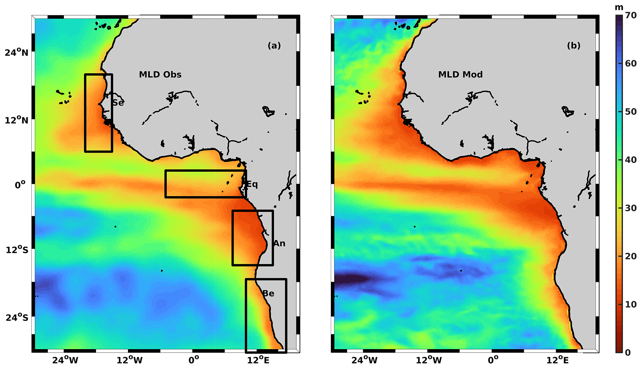
Figure 1 Annual mean of mixed-layer depth from observations (a) and the model (b). The rectangles in (a) correspond to the four regions of study.

The budget computation slightly differs between the observation-based climatology and the model data. All terms are computed online in the NEMO model, explicitly from Eqs. (1) and (2), except for the entrainment term that is estimated (using the online advection term) as a residual. In the PREFCLIM observed climatology, equations for the heat and salt budgets are simplified, as done in other studies (Stevenson and Niiler, 1983; Foltz et al., 2003, 2004; Delcroix and Henin, 1991; Schlundt et al., 2014). Only the tendency, surface heat or freshwater flux (term A), and advection terms (term B) are computed explicitly, following Eqs. (1) and (2). The residual is composed of unresolved vertical processes like diapycnal heat and salt fluxes, runoff contribution in the case of the salt budget, and accumulated errors from the explicitly resolved terms that can be due to sub-mesoscale activity (Dengler and Rath, 2015). For comparison between observations and the model, terms C and D in Eq. (1) as well as terms C, D, and A^′ in Eq. (2) are grouped in a model pseudo-residual term equivalent to the observation residual. The daily NEMO model online budget terms, available on a 0.25^∘ grid, are resampled at the lower spatial resolution ($\mathrm{2.5}{}^{\circ }\times \mathrm{2.5}{}^{\circ }$) and time resolution (monthly) of observed budget terms for comparison. The online computation in the model means that the advection term includes high-frequency mesoscale activity. To remove this part and to mimic the resolution of the gridded observations used for the PREFCLIM advection terms, horizontal heat and salt advection terms are also recomputed offline, following Eqs. (1) and (2), with monthly model outputs of currents as well as temperature and salinity resampled at 2.5^∘ resolution. This approach has been used in another salinity budget in the tropical Pacific (Hasson et al., 2013). In addition, a new pseudo-residual is inferred from Eqs. (1) and (2) where advection is calculated offline and called the offline pseudo-residual. In order to evaluate the consistency between the PREFCLIM and NEMO mixed-layer budget climatology, we use common statistics of root mean square deviation (RMSD), standard deviation, and spatial and temporal correlations (r), and we summarize them using Taylor diagrams (Taylor, 2001).

3 Results

3.1 Mixed-layer properties

A preliminary validation of the NEMO regional simulation is done by comparing modeled and observed annual means of mixed-layer depth, mixed-layer temperature, and mixed-layer salinity, as well as the standard deviation of the latter two. The model (Fig. 1b) reproduces the large-scale properties of observed MLD (Fig. 1a) in the eastern tropical Atlantic. In both observations and the model, the shallowest mixed layer is found along the Equator and the coasts of Africa, while the deepest mixed layer is found towards the northern and southern subtropical gyres. The main differences between the modeled and observed MLD are found along the northern coast of the Gulf of Guinea and along 24^∘ S where the model MLD is shallower and along 12^∘ S where the model MLD is deeper (see Fig. A1 in the Appendix). Also, the MLD spatial variations are smoother in the observed product than in the model, despite a similar 0.25^∘ spatial resolution. This is likely due to the fact that the observations underestimate spatial variability because they are not available at the necessary resolution.

The model (Fig. 2b) reproduces the observed mean SST (Fig. 2a) in the eastern tropical Atlantic well. The highest SST is found along the zonal band between 0 and 12^∘ N, while the lowest SST is found in the Benguela and Canary Current regions south of 12^∘ S and north of 18^∘ N, respectively, which are characterized by eastern boundary upwelling systems (EBUSs, Chavez and Messié, 2009). The coastal cooling in the Benguela region is weaker in the model. The cooling associated with the smaller coastal upwelling region north of the Gulf of Guinea (Djakouré et al., 2014, 2017) appears in the model only. The model and observations show similar large-scale patterns of SST seasonal variability (Fig. 2c–d) with an open-ocean minimum between 12^∘ S and 12^∘ N, at the coast around 24^∘ S and 24^∘ N, and maximum variability in the open ocean south of 24^∘ S, at the coast around 15^∘ N and 12^∘ S. However, the model shows a smaller coastal seasonal variability of SST at 12^∘ S compared to the PREFCLIM climatology and a larger variability in the open ocean south of 24^∘ S, and it captures the variability associated with the coastal upwelling north of the Gulf of Guinea that does not appear in PREFCLIM. These differences are probably associated with the strengths and weaknesses in the two data sources. On the one hand, there is variable observational coverage, from the very densely sampled EAF-Nansen data along the shore to generally lower observational coverage in the regions away from the shores. On the other hand, the wind forcing used for the model may not allow fully capturing the nearshore variability (Junker et al., 2015).

The model (Fig. 3b) also represents the main observed features of SSS (Fig. 3a) in the eastern tropical Atlantic. The highest SSS is found towards the center of both the northern and southern subtropical gyres. In contrast, the lowest SSS is found slightly north of the Equator and in the Gulf of Guinea due to the strong precipitation associated with the ITCZ and river runoff. SSS is also relatively low in the Benguela upwelling region. SSS is lower in the model than in observations in the eastern part of the Gulf of Guinea, but higher along 12^∘ S (see Fig. A1). Except for the Benguela region, the model (Fig. 3d) shows a strong SSS variability associated with low-SSS regions. However, the PREFCLIM climatology (Fig. 3b) shows a much weaker variability than the model in the Gulf of Guinea and around the Niger River in particular. This may be due to a poor temporal resolution of SSS observations available here. Off the Niger River mouth, the model is in better agreement with other observation-based SSS products, showing a strong (∼2 psu) variability here (Da-Allada et al., 2014).

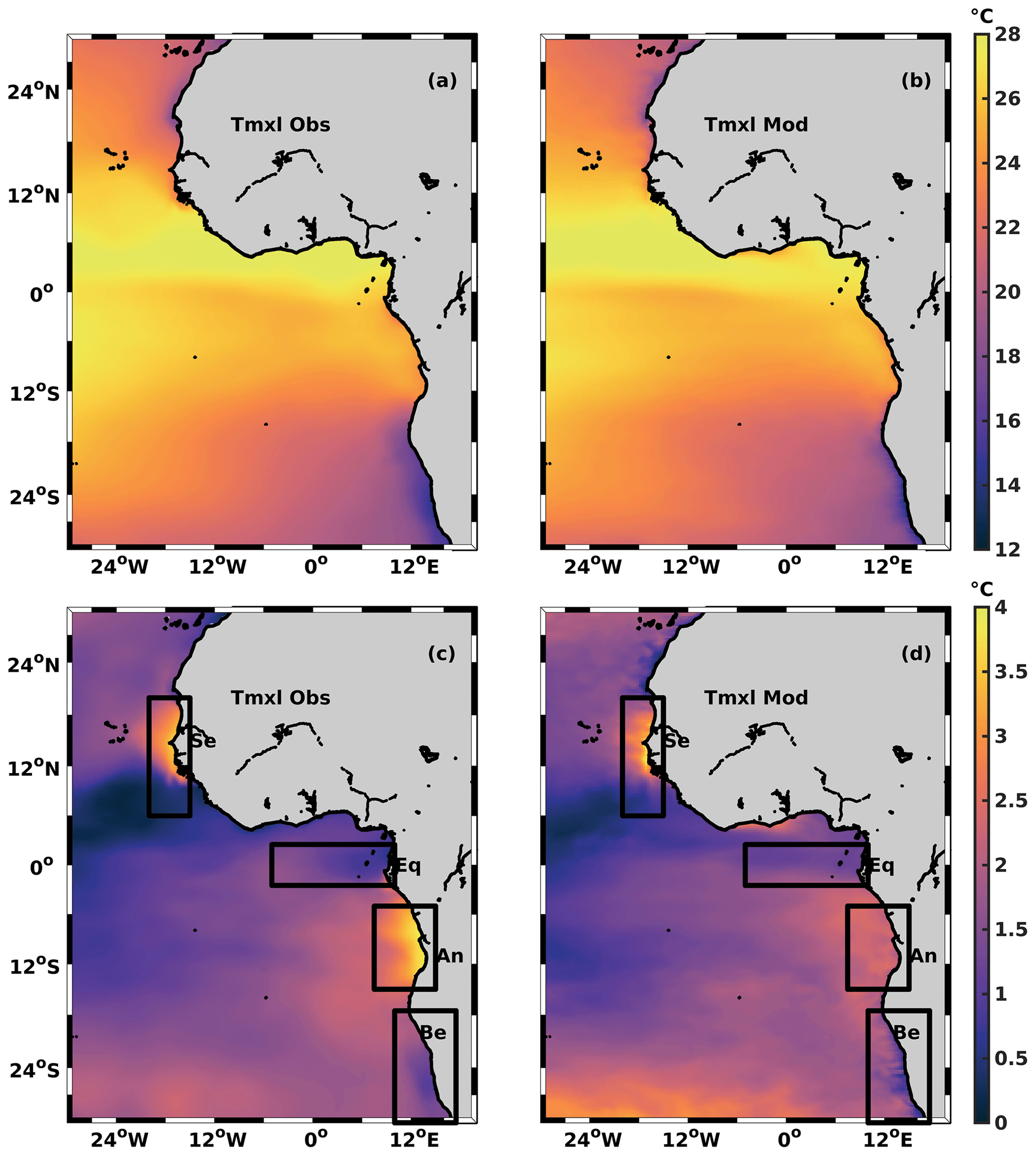
Figure 2 Annual (a, b) and standard deviation (c, d) of mixed-layer temperature from observations (a, c) and the model (b, d). The rectangles in the bottom panels correspond to the four regions of study.

In the following part, the heat and salt budgets will be investigated in detail for four boxes, covering oceanic regions of similar size, selected for their particularly low mean SST and SSS and/or strong SST and SSS variability, as well as generally being associated with upwelling. These are, from north to south, the Senegal box (6–20^∘ N, 20–15^∘ W), the equatorial box (2.5^∘ S–2.5^∘ N, 5^∘ W–10^∘ E), the Angola box (15–5^∘ S, 7.5–15^∘ E), and the Benguela box (30–17.5^∘ S, 10–17.5^∘ E) (Figs. 1–3). Note that these boxes result from a trade-off as we choose to keep the same boxes for heat and salt budgets for consistency. The equatorial and Angola boxes include areas of high and low variability in SSS. The eastern half of the equatorial box is more influenced by the Niger and Congo River plumes than its western half (Jouanno et al., 2011; Da-Allada et al., 2017). The northern half of the Angola box is more influenced by the Congo River plume than its southern half, as mentioned by Awo et al. (2022).

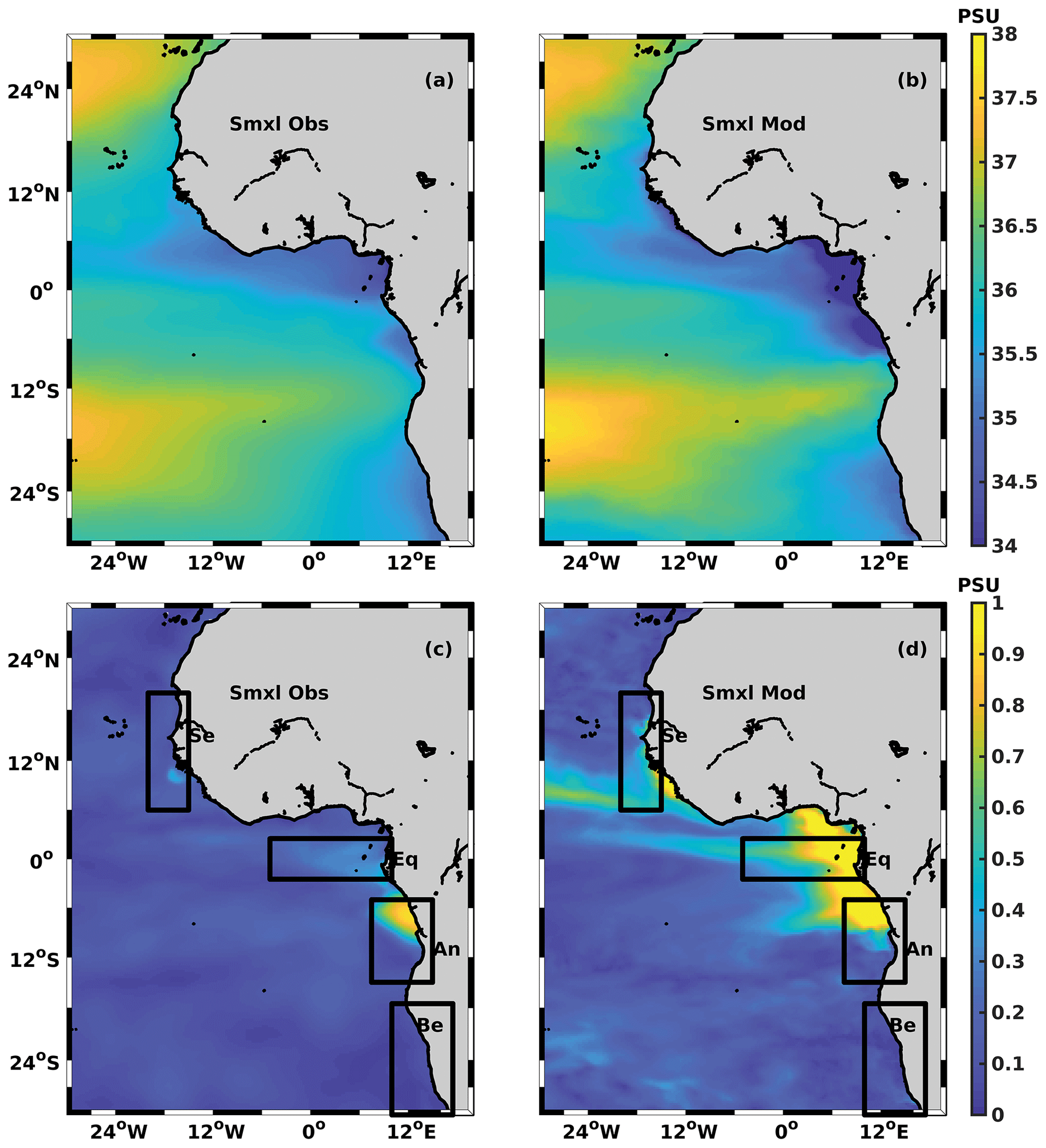
Figure 3 Annual mean (a, b) and standard deviation (c, d) of mixed-layer salinity from observations (a, c) and the model (b, d). The rectangles in the bottom panels correspond to the four boxes of study.

3.2 Mixed-layer heat budget

3.2.1 Time-averaged spatial variations

We compared the mean mixed-layer heat budget from the model and observations. The surface heat flux and horizontal heat advection maps are presented in Fig. 4. Surface heat flux from observations is positive everywhere in the eastern tropical Atlantic, with a maximum along the Equator that gets the strongest solar flux, and along the west coasts of Africa (Fig. 4a). Along West African coasts, the heat flux is strong as solar flux can concentrate in a thin mixed layer (Fig. 1), notably due to the strong salinity stratification induced by the Niger and Congo rivers in the Gulf of Guinea. In addition, the temperature difference between the ocean cooled by coastal upwelling (Benguela, Senegal, see Fig. 2) and the atmosphere leads to a reduced latent heat flux. The model reproduces the observed patterns with higher resolution (Fig. 4c) and, when resampled similarly (Fig. 4b), shows good spatial agreement with the PREFCLIM climatology (r=0.85). The seasonal variations of the NEMO and PREFCLIM heat fluxes are also very well correlated except along the Equator (Fig. 4d). However, the NEMO model flux is biased low compared to PREFCLIM. It shows a net flux towards the atmosphere along zonal bands around 6^∘ N and 12^∘ S. These differences can be explained by the different data sources used for surface heat flux in the PREFCLIM climatology (TropFlux) and as forcing for the NEMO model (DFS5.2), but also due to the feedback of simulated oceanic conditions on the heat fluxes through bulk formulae in the model.

As expected, there are important differences between the maps of offline heat advection, calculated based on the coarsened model currents and hydrography (Fig. 4f), and the online heat advection taking into account the full spatiotemporal variability (Fig. 4g, resampled to 2.5^∘ after calculating advection). In the online version, advection acts to cool the mixed layer in a thinner western equatorial band and to mainly warm the mixed layer in a larger part of the Gulf of Guinea. The offline advection is in much better agreement with the PREFCLIM climatology than the online advection (spatial correlation coefficient r=0.54 vs. r=0.08). In PREFCLIM (Fig. 4e), the distributions of horizontal heat advection and surface heat flux are approximately opposite each other, with advection acting to cool the mixed layer along most of the 3^∘ S–3^∘ N band and along the coast. This sign is expected off the EBUSs of Senegal and Benguela as temperature decreases towards the coast (eastward) and the zonal circulation is dominated by the westward North Equatorial Current and South Equatorial Current (NEC and SEC). The seasonal variations of the PREFCLIM and NEMO offline advection terms show correlations quite different from one place to another that are moderate on average but rather large slightly south of the Equator (Fig. 4h). We also compared the annual mean spatial distribution from the two versions of model advection to the Lagrangian advection and found that the offline advection is also much better correlated than the online advection (r=0.58 versus r=0.37) with the Lagrangian advection terms (see Fig. A2 for more details), which suggests that Lagrangian float density is not sufficient or homogenous enough to capture nonlinear advection terms.

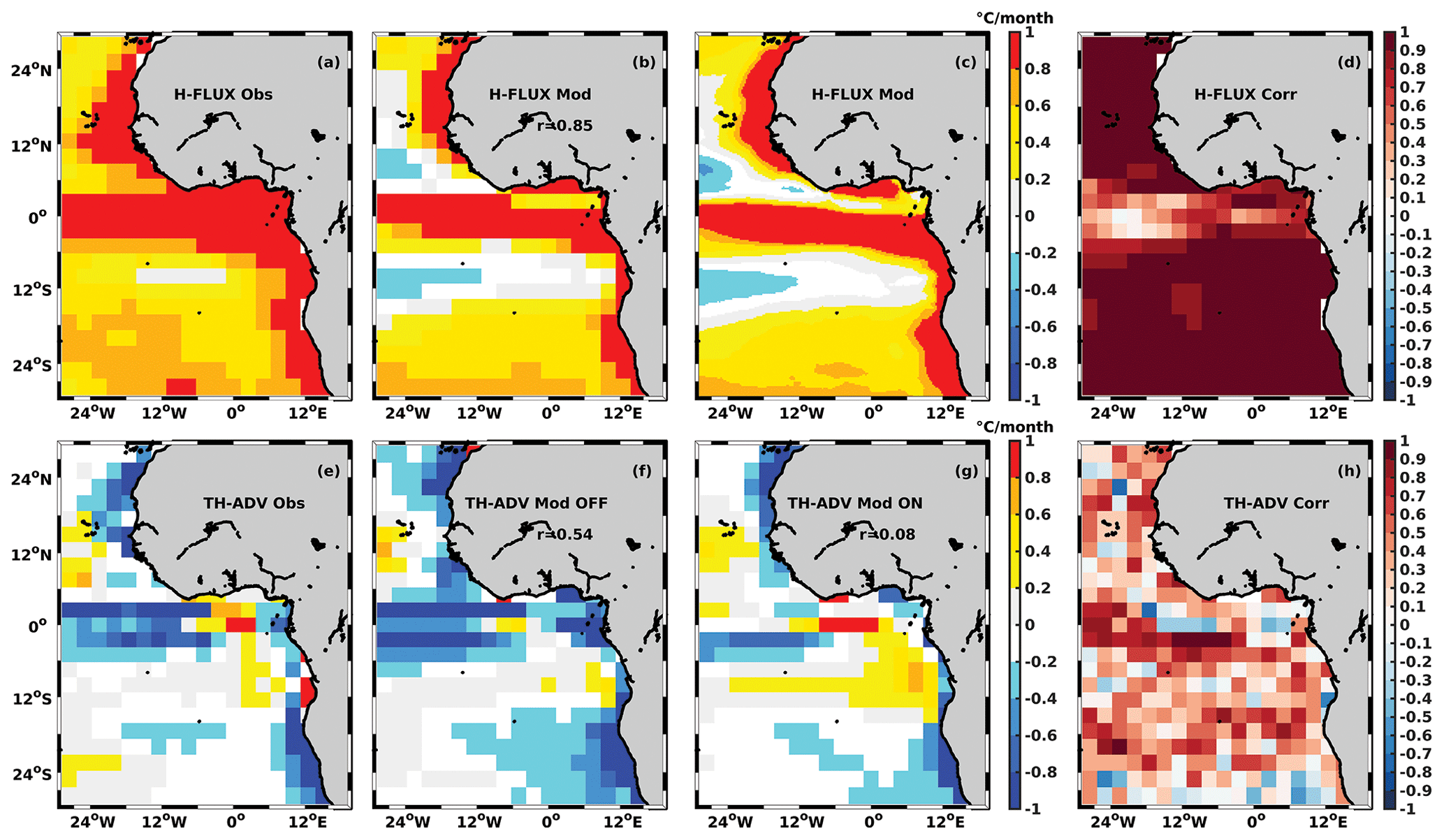
Figure 4 Mean heat flux from PREFCLIM (a), NEMO resampled at PREFCLIM 2.5^∘ resolution (b) or at original 0.25^∘ resolution (c), and seasonal correlation between PREFCLIM and NEMO heat flux (d). Mean horizontal heat advection from PREFCLIM (e), NEMO offline (f) or online computation resampled to 2.5^∘ resolution (g), and seasonal correlation between PREFCLIM and NEMO offline advection (h). r in (b), (f), and (g) indicates the spatial correlation between PREFCLIM and NEMO, which is 95 % significant when r>0.12. The temporal correlation of seasonal cycles in (d) and (h) is 95 % significant when r>0.58.

3.2.2 Regional seasonal budget

In this part, we analyze the individual contributions of different physical processes to the heat budget during a seasonal cycle in selected regions. We present the seasonal variability of mixed-layer temperature and of the heat tendency term (Fig. 5) and try to identify the dominant processes. Taylor diagrams are used to evaluate the consistency of the global terms of the budget between PREFCLIM climatology and the NEMO model (Fig. 6). In the following, the observed gridded advection, rather than the observed Lagrangian advection, is used because it is generally better correlated with the model advection (see Figs. A3 and A4 for more details).

In the Senegal region, observed and modeled seasonal mixed-layer temperature variations (Fig. 5a) are largely consistent (r=0.96, RMSD = 0.64 ^∘C). They both show an annual cycle with an SST maximum around 27 ^∘C in September and a minimum of around 22 ^∘C in the middle of the October–May upwelling season (Ndoye et al., 2014). The minimum is, however, found 1 month later in the model (March) than in the observations (February). The related tendency terms from observations and the model (Fig. 5a) agree to a lesser extent (r=0.91 and RMSD = 0.43 ^∘C per month), which is mainly present in May–June when the modeled warming is larger than the observed warming. The PREFCLIM and the modeled regional heat budgets (Fig. 5b) agree on the seasonal variations of heat flux (r=0.97 and RMSD = 0.24 ^∘C per month). Differences between observations and the model are larger for horizontal advection, and again offline advection from NEMO compares slightly better than online advection with PREFCLIM (r=0.52, RMSD  = 1.34 ^∘C per month vs. r=0.46, RMSD = 0.99 ^∘C per month, see Fig. A3 for more details). The (pseudo-)residual terms, however, compare better for online advection than for offline advection (r=0.96 and RMSD = 0.72 ^∘C per month vs. r=0.51 and RMSD = 0.87 ^∘C per month, respectively). Overall, in the Senegal region, the seasonal cycle of mixed-layer temperature is mainly controlled by surface heat fluxes that are strong and drive the warming from March to September. For the rest of the year, they are small or negative and, with the help of horizontal advection and vertical diffusion, induce cooling (Fig. 5c).

In the equatorial region, Fig. 5d presents the seasonal evolution of mixed-layer temperature in the model and observations. There is a strong consistency (with r=0.98 and RMSD = 0.28 ^∘C) between the two terms, with an SST minimum in the same month of August, while the model reaches the SST maximum in April, 1 month after the observations. Temperature tendency terms are also consistent (r=0.94 and RMSD = 0.27 ^∘C per month), although the maximum cooling in May is strongest in the model. We note also a relatively good consistency in the seasonal cycle of the heat flux (Fig. 5e, r=0.78 and RMSD = 1.14 ^∘C per month). There is much less agreement between NEMO and PREFCLIM for the horizontal advection term, whether it is computed online (r=0.15 and RMSD = 1.37 ^∘C per month) or offline ($r=-\mathrm{0.69}$ and RMSD = 4.27 ^∘C per month) in the model. The observed residual term compares much better with the model online pseudo-residual term (r=0.83 and RMSD = 0.56 ^∘C per month) than with the offline pseudo-residual (r=0.11 and RMSD = 1.15 ^∘C per month). Overall, in this equatorial box, according to the model the seasonal cycle of mixed-layer temperature is essentially driven by vertical heat diffusion (Fig. 5f) as its variations are rather similar to those of the temperature tendency term, except for a shift that can be explained by the heat flux, which remains positive and relatively constant all year long.

In the Angola region, the model reproduces the seasonal evolution of observed mixed-layer temperature well (Fig. 5g, r=0.96 and RMSD = 0.86 ^∘C). The maximum SST observed in March is lagged by 1 month in the model, but the minimum SST is found in August in both NEMO and the PREFCLIM climatology. Differences are relatively larger for the heat tendency term (r=0.84 and RMSD = 0.80 ^∘C per month) that is smaller in the model than observed in November–December (Fig. 5g). We note strong agreement between modeled and observed heat flux (Fig. 5h, r=0.97 and RMSD = 0.24 ^∘C per month). On the contrary, horizontal heat advection terms are poorly correlated when computed online in the model (r=0.05 and RMSD = 1.04 ^∘C per month), but we observe an improvement when computed offline (r=0.44 and RMSD = 0.90 ^∘C per month). This suggests an important role of nonlinear terms in the heat budget. The resulting observed residual term and model (online and offline) pseudo-residual term are also quite different (respectively r=0.51 and RMSD = 0.90 ^∘C per month and r=0.44 and RMSD = 0.89 ^∘C per month). In the Angola box, the seasonal cycle of the mixed-layer heat budget is mostly controlled by heat fluxes, especially solar fluxes, with a contribution from zonal advection and vertical diffusion (Fig. 5i).

In the Benguela region (Fig. 5j), the model reproduces the observed seasonal cycle of the mixed-layer temperature well, which is maximum in February–May and minimum from July to October, but with a positive bias close to 1 ^∘C (r=0.97, RMSD = 0.82 ^∘C). The heat tendency term of the model agrees with observations (Fig. 5j, r=0.95 and RMSD = 0.25 ^∘C per month). Heat flux variations are very well correlated (Fig. 5k, r=0.99, RMSD = 1.16 ^∘C per month). Horizontal heat advection variations are moderately correlated for offline computation (r=0.70, RMSD = 0.90 ^∘C per month) and even for online computation (r=0.68, RMSD = 1.11 ^∘C per month), and the observed residual and modeled pseudo-residual are also consistent (r=0.73, RMSD = 0.68 ^∘C per month vs. r=0.60, RMSD = 0.82 ^∘C per month for online and offline version, respectively). In the Benguela region, the heat budget seasonal cycle is largely controlled by heat flux warming, balanced by the cumulative cooling effect of zonal heat advection and vertical diffusion (Fig. 5l).

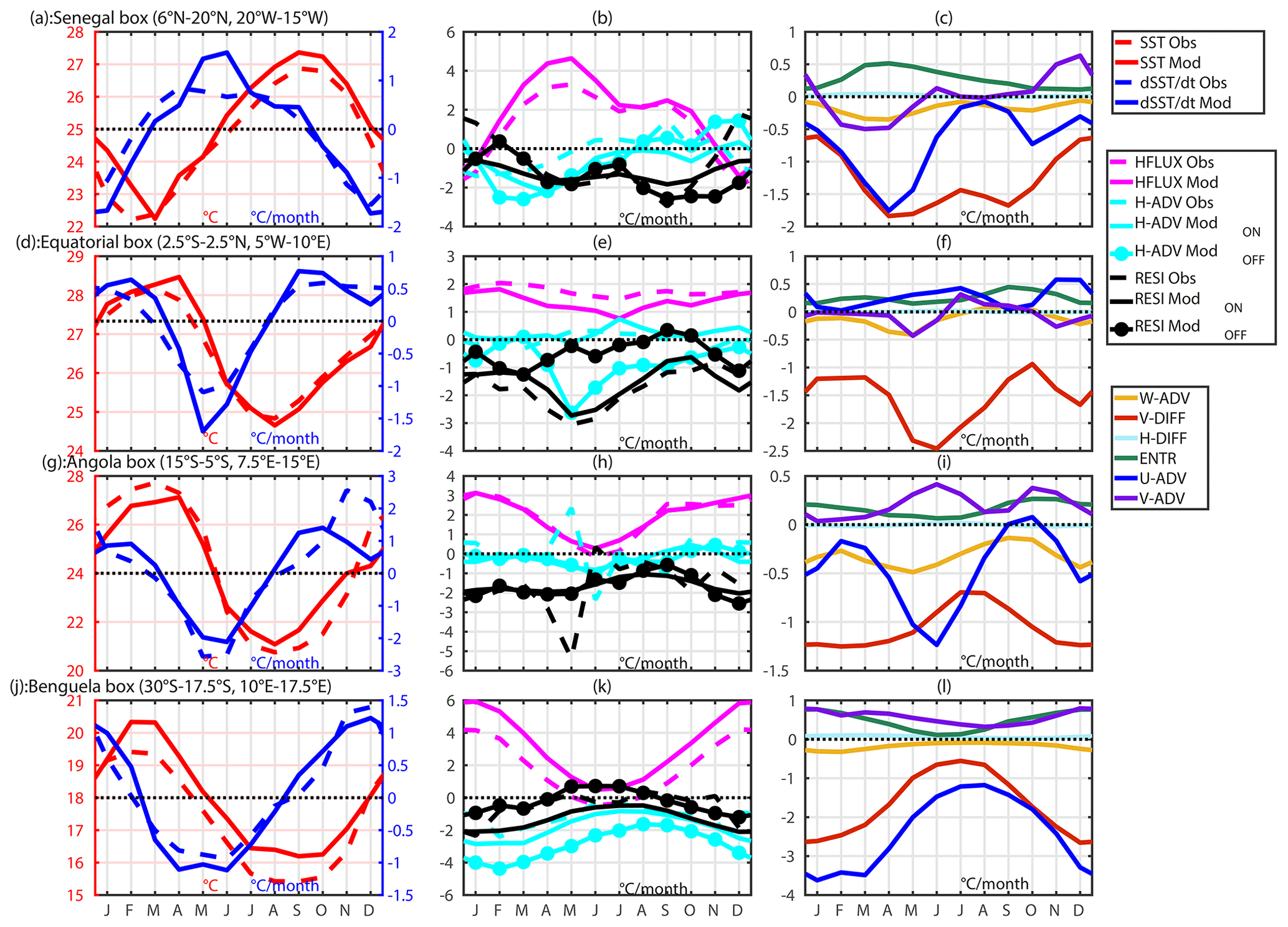
Figure 5 Seasonal mixed-layer heat budget terms from observations (dashed line) and the model (full line and full dotted line for pseudo-residual associated with offline advection) in selected regions: SST (^∘C) and tendency terms (^∘C per month).

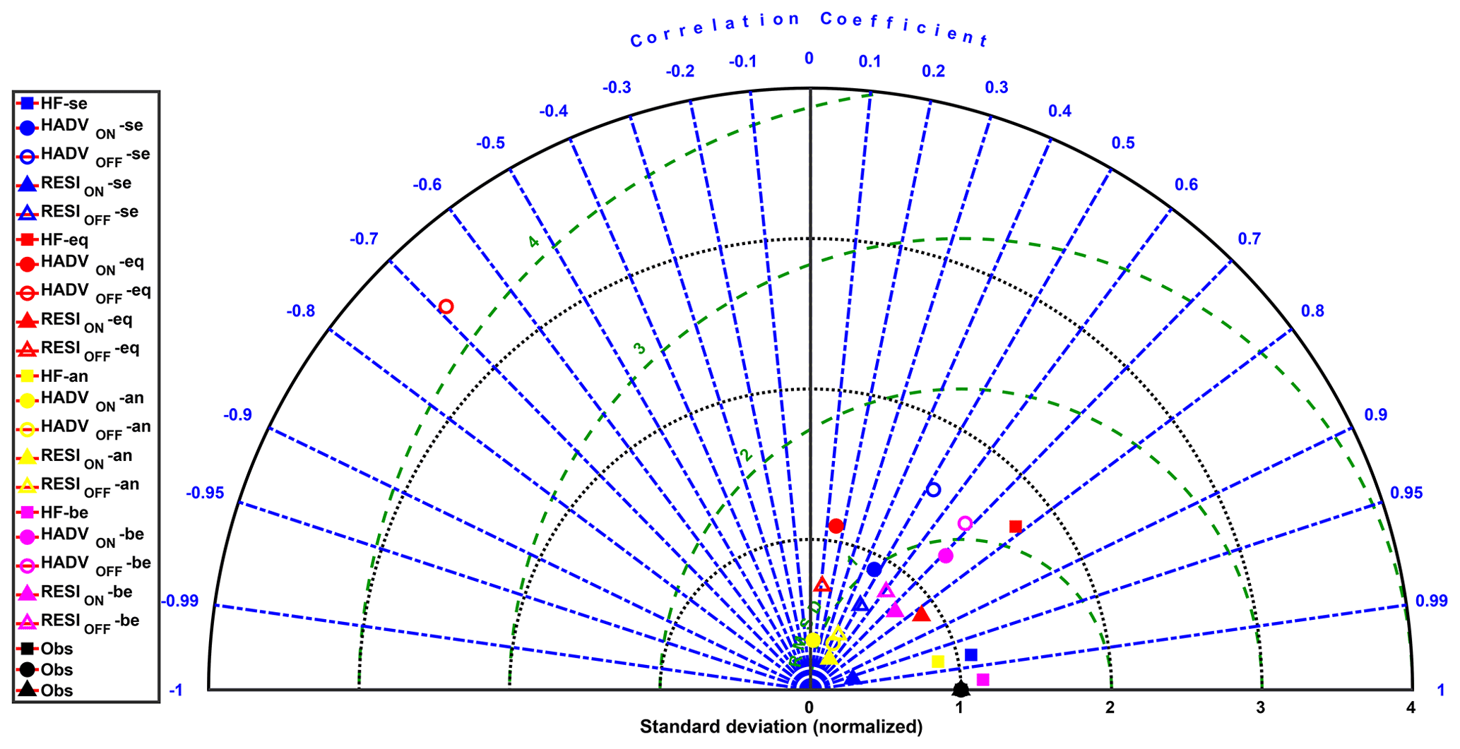
Figure 6 Taylor diagram of global terms of the heat budget in selected regions. Heat flux, horizontal advection (gridded advection for observations and online advection for model), and (pseudo-)residuals are represented by squares, circles, and triangles, respectively. Empty circles and triangles are offline advection and associated (pseudo-)residuals. Senegal, Benguela, equatorial, and Angola regions are designed by blue, red, yellow, and magenta, respectively. Correlations are 95 % significant when r>0.58.

3.3 Mixed-layer salt budget

3.3.1 Time-averaged spatial variations

We now compare the mean salt budget from the model and from observations through freshwater flux and horizontal salt advection (Fig. 7). The PREFCLIM freshwater flux acts to decrease the mixed-layer salinity along the 0–12^∘ N equatorial band, dominated by strong precipitation due to the ITCZ (Fig. 7a). Elsewhere in the eastern tropical Atlantic, freshwater flux is dominated by evaporation, which acts to increase mixed-layer salinity, a feature of the northern and southern subtropical gyres. Evaporation is maximum off Angola, where southern trade winds can enhance it. The model freshwater flux forcing reproduces these patterns and, when resampled to the PREFCLIM resolution (Fig. 7b), shows good spatial agreement with the PREFCLIM climatology (r=0.96). However, the NEMO freshwater flux shows a negative bias along the 6–12^∘ N band and in the Gulf of Guinea and a high positive bias in the rest of the eastern tropical Atlantic basin. These differences are likely due to the different data sources used for surface freshwater flux in the PREFCLIM climatology (TropFlux for evaporation and GPCP for precipitation) and as forcing for the NEMO model (DFS5.2). However, the seasonal variations of freshwater flux are generally well correlated between NEMO and PREFCLIM except for a few regions (Fig. 7d). As expected, there are important differences between the maps of offline salt advection (Fig. 7f) and online salt advection (Fig. 7g, resampled at 2.5^∘). In the online version, advection strongly acts to decrease mixed-layer salinity almost everywhere in the eastern tropical Atlantic. However, we note that in the offline version (Fig. 7f) and in observations (Fig. 7e), advection acts to increase salinity for some regions: in the 4–10^∘ N equatorial band, west of 12^∘ W between 30 and 18^∘ S, off Angola, and in the northern Gulf of Guinea. The spatial distribution of offline advection is in much better agreement with the PREFCLIM climatology than online advection (r=0.48 vs. r=0.17). Schematically, in the eastern tropical Atlantic, salinity increases poleward from the Equator due to strong evaporation in the subtropical gyres, which drives the meridional gradient (Fig. 3a–b). In addition, salinity decreases toward the east because of freshwater intakes from rivers in the Gulf of Guinea, resulting in a westward increase in SSS. In the Gulf of Guinea, the observed salinity increase by advection can be explained by this SSS gradient transported by the eastward southern Guinea Current (GC), following Eq. (2). The freshening by advection in a large part of the eastern tropical Atlantic basin is expected as the circulation is, on the contrary, dominated by the westward NEC and SEC. In addition, the presence of alongshore currents like the southward Angola Current and northward Benguela Current in these coastal regions can drive either a salting or a freshening due to horizontal salt advection, as shown with NEMO. Moreover, there can be competition between zonal and meridional salt advection (Da-Allada et al., 2013). The correlation between seasonal cycles of advection in NEMO and PREFCLIM is very dependent on the location, but it is generally stronger in the Gulf of Guinea and toward the subtropical gyres (Fig. 7h). We also compared the annual mean spatial distribution from the two versions of model advection to the Lagrangian advection and found that the offline advection is also much better correlated than the online advection (r=0.51 versus r=0.15) with the Lagrangian advection. This suggest the importance of nonlinear terms. More statistics on comparison of zonal and meridional advection terms can be found in Fig. A3.

Figure 7 Mean freshwater flux from PREFCLIM (a), NEMO resampled at PREFCLIM 2.5^∘ resolution (b) or at original 0.25^∘ resolution (c), and seasonal correlation between PREFCLIM and NEMO freshwater flux (d). Mean horizontal salt advection from PREFCLIM (e), NEMO offline  (f) or online computation resampled at 2.5^∘ resolution (g), and seasonal correlation between PREFCLIM and NEMO offline advection (h). R in (b), (f), and (g) indicates the spatial correlation between PREFCLIM and NEMO, which is 95 % significant when r>0.12. The temporal correlation of seasonal cycles in (d) and (h) is 95 % significant when r>0.58.

3.3.2 Regional seasonal budget

As previously done for the heat budget (see Figs. A5 and A6 for more details), we evaluate the individual contributions of different physical processes to the salt budget during a seasonal cycle (Fig. 8) and try to identify the dominant processes. Taylor diagrams are used to evaluate the consistency of budget terms between PREFCLIM climatology and the NEMO model (Fig. 9).

In the Senegal region, observed and modeled mixed-layer salinity seasonal cycles (Fig. 8a) are very different (r=0.59, RMSD = 0.33 psu). SSS variations are around 0.1 psu during the seasonal cycle in observations, but reach 0.7 psu in the model, with a maximum in May and a minimum in October (the latter also seen in observations). The SSS increase from October to May coincides with the upwelling season (Ndoye et al., 2014). The seasonal variations of the tendency salinity terms (Fig. 8a) are also quite different (r=0.55, RMSD = 0.12 psu per month). The observed term remains weaker than the modeled term; they vary in opposite phase from December to March, then in phase from this month on, but the modeled freshening is larger than observed in May–November. However, the seasonal variations of freshwater flux (Fig. 8b) show good agreement between observations and the model (r=0.99, RMSD = 0.39 psu per month). Modeled horizontal salt advection and observed horizontal salt advection are less correlated (r=0.51, RMSD = 1.34 psu per month for online vs. r=0.57, RMSD = 3.87 psu per month for offline), and there are very large differences ($r=-\mathrm{0.19}$, RMSD = 1.65 psu per month for online vs. $r=-\mathrm{0.15}$, RMSD = 4.09 psu per month for offline) between the observed residual term and the model pseudo-residual term. In this region, the balance is controlled in large part by freshwater flux because of the compensation between different oceanic processes. From June to October the observed freshening can be explained by precipitation, which reaches its maximum between July and August because of the ITCZ position over Sahel, and associated runoff, particularly from the Senegal and Gambia rivers. From October to November, the freshening is associated with the combined effect of zonal advection (Fig. 8c), precipitation, and river runoff, in this order. For the rest of the year, evaporation plays a dominant role and increases mixed-layer salinity.

In the equatorial region, the modeled and observed seasonal cycles of the mixed-layer salinity are largely in phase (Fig. 8d, r=0.82, RMSD = 0.79 psu), but the modeled salinity has a seasonal cycle 3 times stronger and is lower by almost 1.5 psu between April and May. This could be due to the fact that the observations miss some strong and very shallow near-surface stratification, which is averaged into the surface grid box of the model. The minimum SSS observed in February is lagged by 2 months in the model, but the maximum SSS is found in October in both NEMO and the PREFCLIM climatology. The related tendency terms (Fig. 8d) are weakly correlated (r=0.58, RMSD = 0.27 psu per month). The model term has a stronger amplitude throughout the cycle with some peaks in January, May, and November. Figure 8e shows that freshwater fluxes are strongly correlated (r=0.94, RMSD = 0.90 psu per month). The horizontal advection terms are quite different when online computation is used (r=0.38, RMSD = 4.03 psu per month) but compare better with the offline advection (r=0.77, RMSD = 8.56 psu per month), although the modeled advection in both cases shows stronger variations than observed. The model pseudo-residual also compares better with the observed residual for the offline version than for the online version (r=0.81, RMSD = 3.51 psu per month vs. r=0.54, RMSD = 1.76 psu per month, respectively). In the equatorial region, the seasonal variability of mixed-layer salinity is mostly due to vertical salt diffusion and zonal salt advection (Fig. 8f). From September to March, zonal salt advection increases mixed-layer salinity. Vertical salt diffusion plays a major role in increasing mixed-layer salinity the rest of the year, in particular in May when it reaches its maximum. The contributions of freshwater flux as well as vertical and meridional salt advection are weak and can compensate for each other during the seasonal cycle. Note that, although the seasonal salt budget described above is representative of the whole equatorial box, SSS variability within the box increases toward the east (Fig. 3) as the magnitude of individual processes increases with the salinity stratification due to coastal river plumes (not shown).

In the Angola region, Fig. 8g presents the seasonal evolution of mixed-layer salinity in the model and observations. The model reproduces (r=0.55, RMSD = 0.28 psu) the seasonal evolution of observed SSS relatively well from the beginning of the year to August. In June, both the observed SSS and modeled SSS are around their maximum, but SSS in the model decreases progressively until it reaches its minimum in November, when the observed SSS only begins to decrease until its minimum in February, the month in which the model reaches its second minimum. The related tendency terms present disagreement above all at the end of the cycle (Fig. 8g, r=0.29, RMSD = 0.27 psu per month). SSS in NEMO reaches its maximum in May and its minimum in February, while observed SSS reaches its maximum in April and its minimum in December when the model shows a secondary maximum. Surface freshwater fluxes are both positive all year long in NEMO and PREFCLIM, indicating that evaporation is stronger than precipitation, with similar variations (Fig. 8h r=0.79, RMSD = 0.66 psu per month). In addition to these freshwater fluxes, there is strong runoff associated with the freshwater discharge from the Congo River that flows in this box, which is a major driver of SSS here (Houndegnonto et al., 2021), included in NEMO only. Horizontal advection in the model and observations is quite different (r=0.15, RMSD = 2.13 psu per month for online version vs. r=0.09, RMSD = 2.51 psu per month for offline version), and the modeled pseudo-residual compares better with the observed residual for the online version (r=0.64, RMSD = 0.78 psu per month) than for the offline version (r=0.38, RMSD = 1.43 psu per month). According to the model, in this region, the salt budget seasonal cycle is mostly driven by oceanic processes, namely meridional advection, vertical diffusion, and advection, in this order (Fig. 8i). Note that, although the seasonal salt budget described above is representative of the whole Angola box, SSS variability within the box increases toward the north (Fig. 3) as the magnitude of individual processes increases with the salinity stratification due to coastal river plumes (not shown).

In the Benguela region, the model follows the observed seasonal cycle of mixed-layer salinity well (r=0.76, RMSD = 0.06 psu), though with a negative mean bias (around −0.06 psu) throughout the cycle (Fig. 8j). The modeled SSS reaches its maximum in May, 1 month later than observed, and its minimum in December, also 1 month later than observed. The salt tendency term of the model also reproduces the observed term relatively well (r=0.68, RMSD = 0.01 psu per month), especially from January to July (Fig. 8j). The model shows a maximum SSS increase in February, 1 month earlier than observed, and maximum SSS decreases in August and December, 2 months later than the observed peaks. NEMO and PREFCLIM freshwater fluxes are consistent (Fig. 8k, r=0.92, RMSD = 0.88 psu per month). Horizontal advection terms are less consistent between observations and the model (r=0.56, RMSD = 0.83 psu per month for online version vs. r=0.15, RMSD = 1.04 psu per month for offline version), as well as the pseudo-residual terms (r=0.50, RMSD = 0.92 psu per month for online version vs. $r=-\mathrm{0.09}$, RMSD = 1.10 psu per month for offline version). In the Benguela region, the salt budget seems to be mostly controlled by freshwater flux and zonal salt advection. The observed freshening from March to December can be partly explained by the minimum of evaporation in June, followed by the increasingly negative effect of zonal advection.

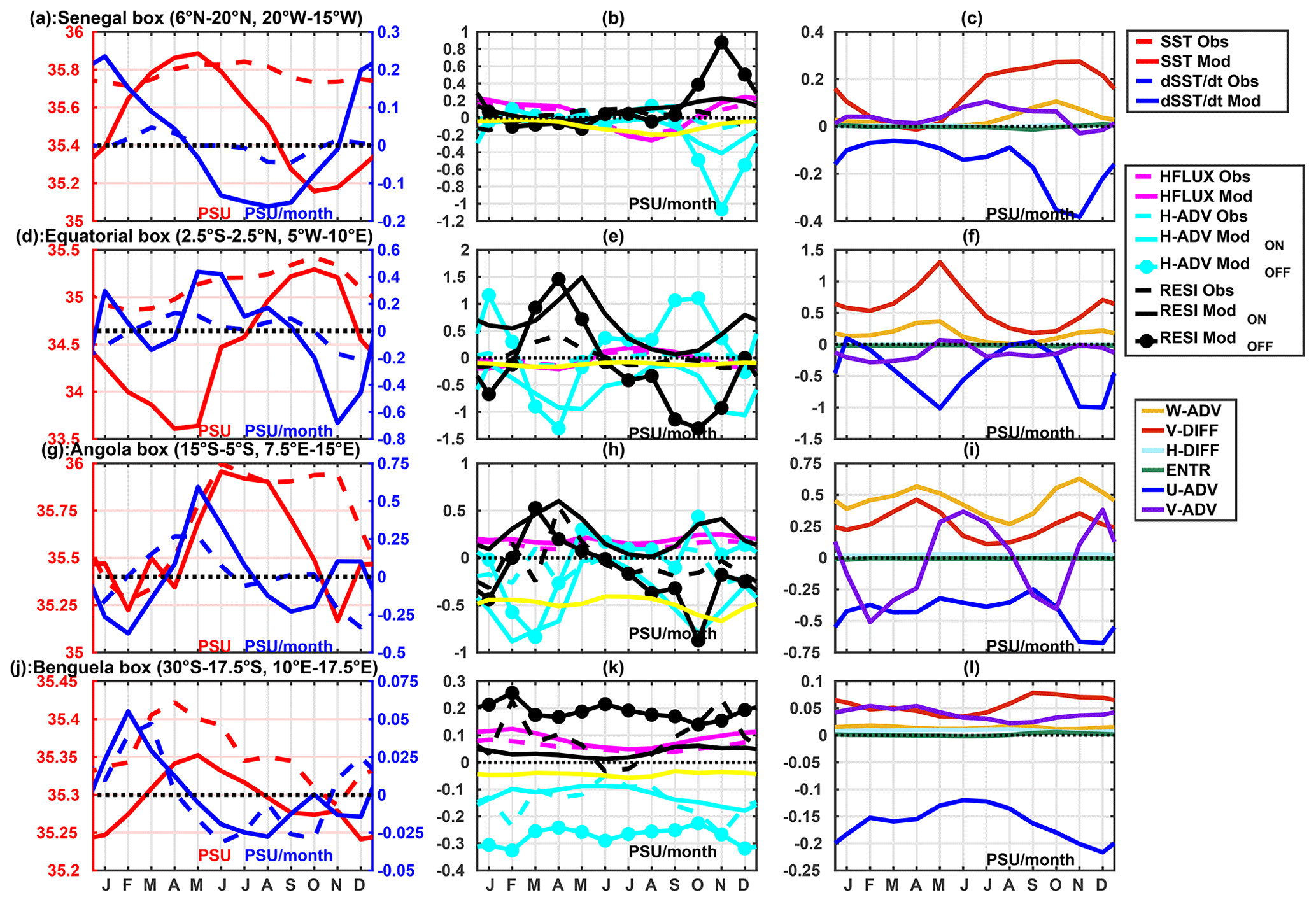
Figure 8 Seasonal mixed-layer salt budget terms from observations (dashed line) and the model (full line and full dotted line for pseudo-residual associated with offline advection) in selected regions: SSS in practical salinity units and tendency terms in practical salinity units per month.

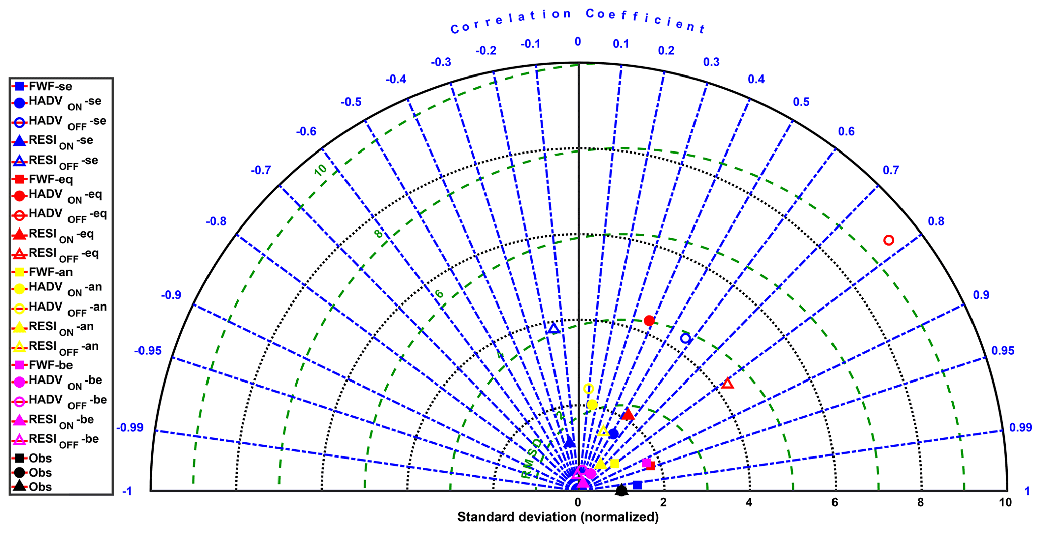
Figure 9 Taylor diagram of global terms of the salt budget in selected regions. Freshwater flux, horizontal advection (gridded advection for observations and online advection for model), and (pseudo-)residuals are represented by squares, circles, and triangles, respectively. Empty circles and triangles are offline advection and associated (pseudo-)residuals. Senegal, Benguela, equatorial, and Angola regions are designed by blue, red, yellow, and magenta, respectively. Correlations are 95 % significant when r>0.58.

4 Discussion and conclusions

In this paper, we examined the dominant physical processes controlling the seasonal variability of mixed-layer heat and salt budgets in selected coastal regions of the eastern tropical Atlantic, namely the Senegal, equatorial, Angola, and Benguela regions. First, we used both a regional configuration of the NEMO model and the PREFCLIM observation-based climatology to analyze the spatial variations of the annual mean mixed-layer heat and salt budgets in the eastern tropical Atlantic (see Figs. 4 and 7, respectively). The model outputs were resampled to the PREFCLIM time–space resolution to compare maps of the mean processes contributing to mixed-layer heat and salt budgets, according to both sources. Second, we analyzed the seasonal variation of the mixed-layer temperature and salinity, their related tendencies, and potential driving processes: heat and freshwater flux, horizontal heat and salt advection, and other processes estimated from observations as a residual but explicitly resolved in the model for the selected regions. As the PREFCLIM climatology does not capture the mesoscale physical processes, we relied on the high-resolution model outputs to evaluate their contribution to the mixed-layer heat and salt budget.

For the preliminary validation, the results have shown that the model consistently reproduces the mean features of observed mixed-layer depth, temperature, and salinity in the eastern tropical Atlantic (see Figs. 1, 2, and 3, respectively). The existing differences between modeled outputs and the PREFCLIM climatology can be explained by the different heat and salt flux products that are used for forcing the model or for estimating the PREFCLIM budget terms. There are also differences in the method to define the MLD. The PREFCLIM climatology uses the algorithm of Holte and Talley (2009), whereas the model uses the density criterion (0.03 kg m⁻³ relative to the density at 10 m depth) recommended by de Boyer Montégut et al. (2004). For example, the observed strong positive bias of mixed-layer salinity in the model relative to observations around 12^∘ S is associated with a positive bias in MLD. Except for these differences, the model and the PREFCLIM climatology capture the shallow nearshore mixed-layer depth along the Equator and the western coast of Africa where our selected regions are localized.

For the secondary validation, we have used both the model and the PREFCLIM climatology to analyze the annual mean of heat and freshwater flux as well as horizontal heat and salt advection. The model heat and freshwater fluxes largely agree with the PRECLIM climatology (Figs. 4a–b and 7a–b, respectively), except for differences in a few regions that can again be due to different flux products or MLD biases. There are important differences between the model heat and salt advection terms computed either offline (Figs. 4f and 7f, respectively), at PREFCLIM spatiotemporal resolution (2.5^∘, monthly), or online (Figs. 4g and 7g, respectively) at high spatiotemporal resolution (0.25^∘, 20 min) with subsequent monthly resampling at 2.5^∘. These differences are explained by the high-frequency variability related to mesoscale and sub-mesoscale dynamics, which is included in the second case but not in the first case. In particular, including mesoscale dynamics leads to warming around the Equator and off the African coast in the southern Atlantic. West of 10^∘ W and slightly north of the Equator, this is consistent with warming of the equatorial cold tongue by horizontal advection linked to TIWs (Jochum et al., 2004; Grodsky et al., 2005; Peter et al., 2006). This also suggests a similar role of eddies in the Angola and Benguela upwelling systems, where a large number of eddies have been detected (Aguedjou et al., 2019). Regarding salinity, mesoscale advection tends to freshen the Gulf of Guinea, probably by westward export through eddies of fresh waters from the Niger and Congo plumes (Houndegnonto et al., 2021).

At seasonal timescales, the monthly mixed-layer heat and salt tendency terms in the selected regions are very weak in both the PREFCLIM climatology and the model compared to individual terms contributing to the heat and salt budgets that tend to compensate for each other, as also found in previous studies (Da-Allada et al., 2013, 2014; Camara et al., 2015).

Surface heat fluxes, especially the solar flux, dominate the seasonal mixed-layer heat budget in the Senegal, Angola, and Benguela regions (Fig. 5b, h, and k, respectively). In the Senegal region, this result, and the secondary contribution of oceanic processes such as vertical diffusion and zonal advection, which add to latent heat flux to drive the observed winter cooling, confirms previous studies (Carton and Zhou, 1997; Yu et al., 2006).

In the equatorial region, the heat flux remains positive and nearly constant throughout the seasonal cycle. This shows the dominance of the shortwave flux that warms the mixed layer from September to April, although this warming weakens between November and December. Although our selected box slightly differs from previous regional studies, this result is in agreement with earlier studies (Peter et al., 2006; Wade et al., 2011). The variability of mixed-layer temperature, in particular the observed spring–summer cooling during the formation of the ACT, is mainly controlled by vertical heat diffusion (Fig. 5e), confirming other studies (Yu et al., 2006; Jouanno et al., 2011). Recently, Scannell and McPhaden (2018) also confirmed the role of turbulent vertical mixing from a PIRATA buoy located at the southeastern edge of the ACT. While it does not compensate for the cooling effect of vertical diffusion, zonal heat advection is positive all year long in the equatorial region, the only one among analyzed regions where it is so. This is the consequence of a negative zonal temperature gradient as the mixed-layer temperature decreases toward the coast, advected by westward currents associated with the SEC. When associated with meridional heat advection, this leads to a positive horizontal heat advection throughout all year except in the month of May. We note a nearly similar variability of horizontal advection in Wade et al. (2011), although this term is negative in their study except for June–July, when we both observe a positive maximum. This difference can be linked to either products used or the criterion used to define the MLD (temperature vs. density criterion) and maybe to the slightly different boxes of study. Jouanno et al. (2017) also found, like us, a permanent warming effect of horizontal advection in an equatorial box shifted west compared to ours using the same model configuration. In our box, according to the model this warming is largely due to mesoscale advection, probably by eddies as TIW activity sharply decreases east of 15^∘ W (Foltz et al., 2003; Peter et al., 2006; Tuchen et al., 2022). There is overall agreement on the dominant role of vertical mixing to cool the mixed layer during ACT formation. This vertical mixing due to vertical diffusion is explained by the strong vertical shear between the Equatorial Undercurrent (EUC) and the SEC in our selected region, as discussed in previous studies (Wade et al., 2011; Jouanno et al., 2011; Hummels et al., 2013; Schlundt et al., 2014). The vertical mixing can also be enhanced by the effects of TIWs on vertical shear (Heukamp et al., 2022).

In the Angola region, the dominant role of heat flux in the mixed-layer heat budget was also found in previous studies (Carton and Zhou, 1997; Yu et al., 2006). In this region, the incoming shortwave flux warms the mixed layer from August until March against the action of latent heat flux. The competition between the shortwave flux and the latent heat flux is also mentioned in Scannell and McPhaden (2018), although at the 6^∘ S, 8^∘ E position, the horizontal advection remains weak in their study. The cooling observed between April and July is due to the decrease in solar radiation, probably due to cloud cover, with the added effect of zonal heat advection. We observe the warmest temperature in March, and the minimum is reached in August, which corresponds to the upwelling season (Ostrowski et al., 2009; Kopte et al., 2017). Although the contribution of zonal heat advection remains weak compared to the solar flux, the variations of zonal heat advection are in phase with the variation of heat tendency throughout the year.

In the Benguela region, the heat tendency variations are roughly in phase with the heat flux variations. The heat budget is mostly driven by the shortwave flux, as found previously in the neighboring southern Angola upwelling system. The cooling that occurs from March to August can be associated with cloud cover, which reduces the incoming solar flux, and also a small contribution of oceanic processes. The observed coldest temperatures correspond to the July–October upwelling season (Hagen et al., 2001; Muller et al., 2014).

There are much larger differences between PREFCLIM and NEMO in the seasonal variations of the mixed-layer salinity (Fig. 8a, d, g, j) compared to temperature. These seasonal variations generally have a larger amplitude and lower minima in the model, as also seen in Fig. 3. This can be due to several factors. First, although the PREFCLIM product benefited from newly available hydrographic data in the Senegal, Angola, and Namibia coastal waters, the data density is still low in the equatorial Gulf of Guinea (Dengler and Rath, 2015), the freshest waters associated with heavy rain as well as the large Congo and Niger River plumes; hence, the largest difference in seasonal salinity variations is in the equatorial box (Fig. 8d). Poor data density can also be associated with a seasonal bias that may prevent capturing the full seasonal cycle. Second, hydrographic profiles, notably those from Argo floats, do not sample the salinity minimum found in the upper few meters of the ocean in regions highly stratified by rain and river plumes, which induces SSS estimations higher than those observed from satellites (Boutin et al., 2016; Houndegnonto et al., 2021). This leads to overestimation of mixed-layer salinity too. Third, while the NEMO model configuration has high vertical resolution in the upper few meters and homogeneous spatial coverage, the way it reproduces mixed-layer salinity highly depends on its freshwater forcing, including river runoff, and its own dynamics that are of course not perfect. Despite these differences between observations and the model, the comparison is instructive.

The Senegal region is the only one among the four analyzed regions where the salt budget is clearly controlled by the surface freshwater fluxes, with an added runoff effect (Fig. 8b). From March to October the observed freshening can be explained by the combined effect of precipitation and Senegal and Gambia rivers inputs. From October to November, zonal salt advection adds its contribution to existing freshwater inputs to freshen the mixed layer. Vertical salt diffusion, with an additional contribution of meridional and vertical salt advection, tends to increase mixed-layer salinity and partly compensates for the previous freshening effect. Although our selected regions are slightly different, these results are consistent with those of Camara et al. (2015). However, in our study, evaporation plays a dominant role in increasing salinity for the rest of the year, even if there is also a weak contribution of oceanic processes. This disagrees with the study of Camara et al. (2015), wherein the contribution of evaporation to the mixed-layer salt budget is very weak compared to our results. This contradiction can be explained by different model configurations as described in Da-Allada et al. (2017). Camara et al. (2015) use for model forcing an older version of the DRAKKAR Forcing Set (DFS4) compared to the one (DFS5.2) used in the present study, and their model has fewer vertical levels than ours (46 vs. 75). They also use a smaller density criterion (0.01 kg m⁻³ for Camara et al., 2015, vs. 0.03 kg m⁻³ in this study to estimate mixed layer depth) and an additional restoring term for salinity in their model.

In the equatorial region, the seasonal variability of mixed-layer salinity is mainly due to oceanic processes as shown in other studies (Da-Allada et al., 2013, 2014). In our study, we found vertical salt diffusion and zonal salt advection as dominant oceanic processes (Fig. 8f). From October to December and March to July, zonal advection is the most important freshening contribution, stronger that precipitation. It is explained by the westward South Equatorial Current (SEC), which transports low-salinity waters from the Gulf of Guinea associated with the Niger and Congo River plumes (Houndegnonto et al., 2021). The major role played by vertical salt diffusion in increasing the salinity in the mixed layer, demonstrated in previous studies (Da-Allada et al., 2014, 2017), is confirmed by our results for boreal spring–summer in particular. This strong vertical salt diffusion is the consequence of the vertical shear between the westward SEC and the eastward EUC (which transports high-salinity waters) but can be reduced by the strong salinity stratification caused by the Niger and Congo River plumes (Jouanno et al., 2011). Note that vertical diffusion, however, is strongly compensated for by zonal advection, above all in May. These results agree with the other studies covering the region despite slight differences in the limits of selected boxes (Berger et al., 2014; Da-Allada et al., 2014, 2017; Camara et al., 2015). Although the contribution of surface freshwater fluxes and runoff remains weak in our study, its seasonal variations follow those described by Da-Allada et al. (2017), with some time lag. During the period when the ITCZ is close to the Equator between November and April, the freshwater flux is dominated by precipitation and decreases the mixed-layer salinity, whereas the rest of the year, the freshwater flux is dominated by evaporation and increases salinity.

As in the equatorial region, horizontal and vertical oceanic processes drive the mixed-layer salinity in the Angola region too (Fig. 8g–i), in agreement with previous studies (Camara et al., 2015; Awo et al., 2022). Meridional salt advection explains most of the variability in salt budget, particularly its semi-annual cycle, as it freshens the mixed layer in February–April and September–October, when the southward Angola Current brings low-salinity water from the Congo River plume (Gordon and Bosley, 1991; Awo et al., 2022). However, for the rest of the seasonal cycle, a combined action of meridional salt advection, vertical salt advection, and vertical salt diffusion increases the salinity of the mixed layer. Although vertical advection is stronger than vertical diffusion, they remain in phase throughout the cycle and act against the runoff and zonal salt advection. Seasonal variations in both vertical salt diffusion and advection are driven by changes in the vertical salinity gradient related to the semi-annual intrusion of low-salinity surface waters (Camara et al., 2015; Awo et al., 2022).

In the Benguela region, individual contributions of physical processes are relatively weak in comparison to the other regions. The mixed-layer salinity variability is partly controlled by freshwater fluxes, particularly evaporation (Fig. 8j–k). Zonal advection remains negative throughout the year, and from March to December, it acts to decrease salinity, against the action of evaporation that is reinforced by vertical salt diffusion between September and December. The increase in salinity corresponds to the upwelling season in the southern part of Benguela upwelling system in summer (Muller et al., 2014).

Although increasing resolution in oceanic models intends to produce more realistic simulations by explicitly resolving mesoscale variability, and models are the only way to estimate all terms of the heat and salt budget in the mixed layer, it is difficult to directly validate such model budgets with in situ data. One problem is that globally available in situ data can only explicitly resolve near-surface horizontal processes, particularly advection, not vertical processes that have to be estimated as a residual. A second problem is that in situ observation density does not allow estimating horizontal advection at the high resolution available from models. Therefore, to be properly compared with those available from observations, model horizontal advection terms must be computed offline at the spatiotemporal resolution of observations. Our results indeed show that the time-averaged spatial distribution of NEMO offline heat and salt advection terms compares much better to PREFCLIM horizontal advection terms than the online heat and salt advection terms. However, when examining the seasonal cycle of horizontal advection in selected boxes, NEMO offline terms do not always compare well with PREFCLIM, sometimes less than online terms. This suggests that temporal coverage of in situ observations is more critical than spatial coverage, particularly for salinity, and especially in coastal areas of Africa where Argo profiles are relatively scarce and in the equatorial region where Lagrangian drifters do not stay long due to Ekman divergence. Another possibility would be to estimate advection from satellite products of SST, SSS, and currents, the latter estimated from altimetry and satellite wind for their geostrophic and Ekman components, respectively (Bonjean and Lagerloef, 2002), which are available at a resolution of a few tens of kilometers and a few days. The new Surface Water and Ocean Topography (SWOT) mission (Morrow et al., 2019) should soon further improve the resolution of geostrophic currents. The Soil Moisture Ocean Salinity High Resolution (SMOS-HR) mission project (Rodriguez-Fernandez et al., 2022) would also help to capture SSS gradients. The often large differences between offline and online advection terms in the model suggest an important role of small-scale ($<{\mathrm{2.5}}^{\circ }$, <1 month) variability, which includes mesoscale activity recently documented in the eastern tropical Atlantic (Aguedjou et al., 2019), including at the Equator where differences are particularly large. Although the model mixed-layer budget validation has some limitations in the present study, our results are generally in agreement with earlier studies of mixed-layer heat and salt budgets in the tropical Atlantic (Foltz et al., 2003; Jouanno et al., 2011; Wade et al., 2011; Da-Allada et al., 2013; Camara et al., 2015). Except for local studies wherein coordinated field measurements and mooring deployment can be combined to close a short-term mixed-layer budget with in situ observations (Farrar et al., 2015; Farrar and Plueddemann, 2019; Vijith et al., 2020), in most regions, one can only use models to close mixed-layer budgets and trust them to quantify the processes hidden in the residual unresolved by global observations.

Appendix A

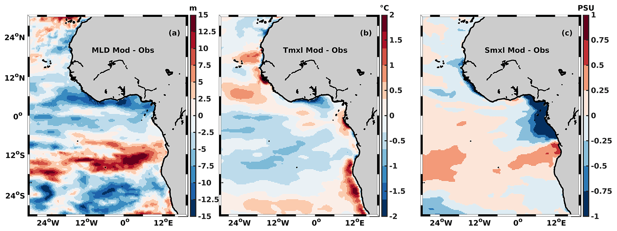
Figure A1 Difference between observations and the model in mixed-layer depth (a), mixed-layer temperature (b), and mixed-layer salinity (c).

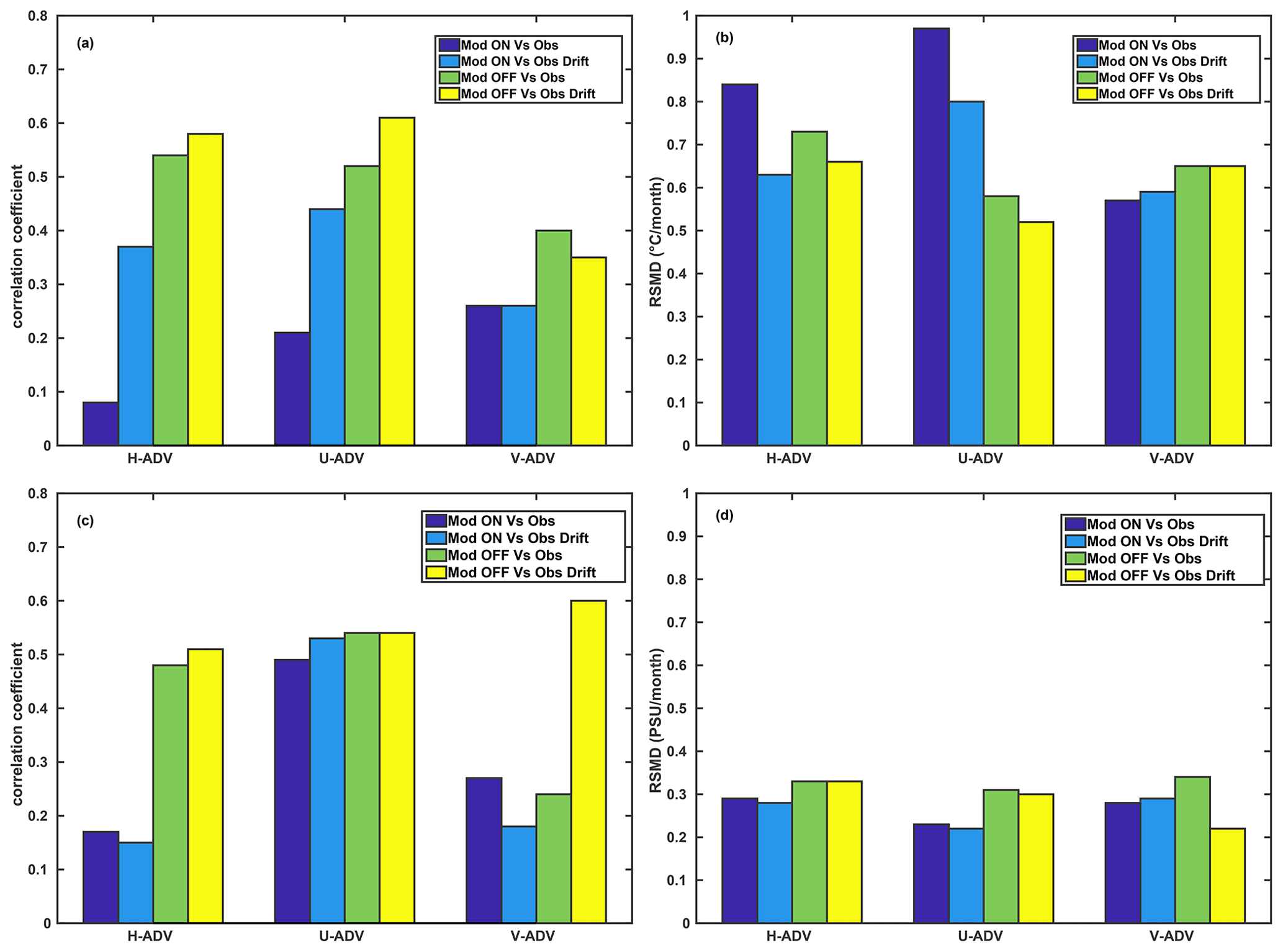
Figure A2 Spatial correlation (r) and RMSD of horizontal, zonal, and meridional heat (a, b) and salt (c, d) advection between observations (Obs and Obs-drift) and the model (online and offline).

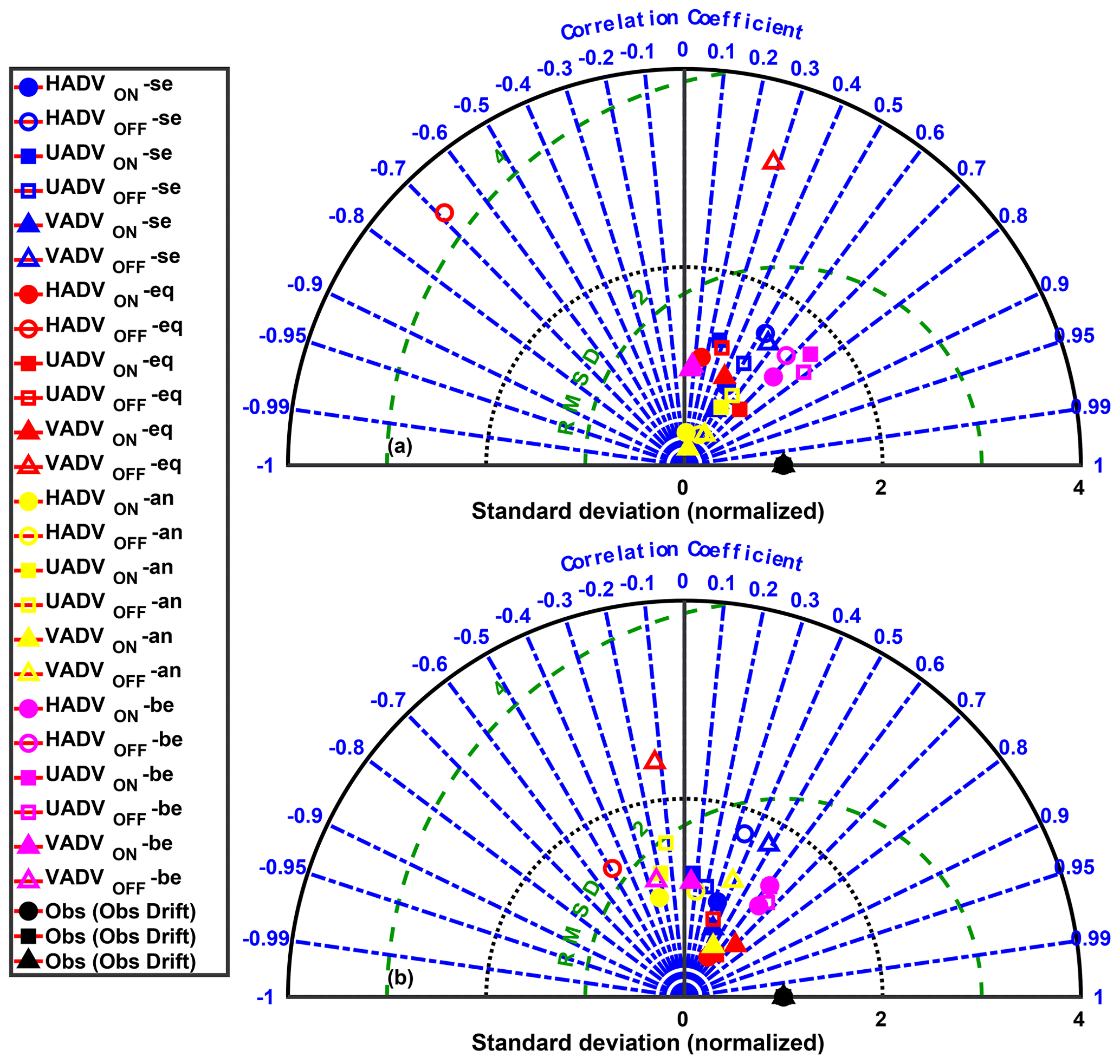
Figure A3 Taylor diagrams comparing seasonal variations of horizontal, zonal, and meridional heat advection (HADV, UADV, VADV) from observations (gridded advection named Obs a; Lagrangian advection named Obs-drift b) and the model (online advection for ON and offline advection for OFF) in the Senegal, equatorial, Angola, and Benguela boxes (blue, red, yellow, and magenta, respectively).

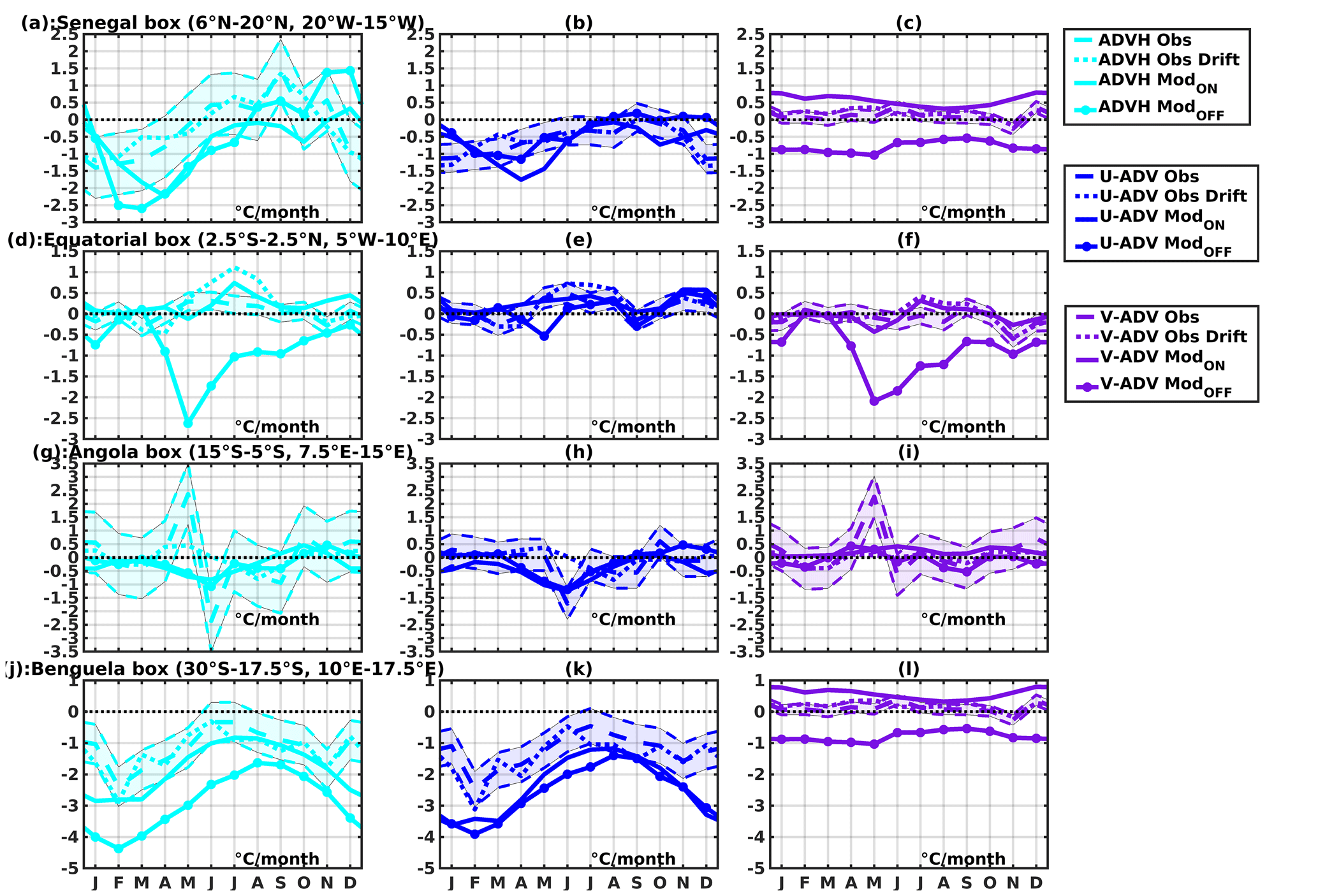
Figure A4 Seasonal cycle of horizontal (cyan), zonal (blue), and meridional (purple) heat advection from observations (dashed line for gridded advection and dotted line for Lagrangian advection) and the model (full line for online and full dotted line for offline) in selected boxes. All others terms are in degrees Celsius per month.

Figure A5 Taylor diagram of horizontal salt advection and these components between observations (gridded advection for Obs a and Lagrangian advection for Obs-drift b) and the model (online for ON and offline for OFF). Senegal, equatorial, Angola, and Benguela boxes are designated by blue, red, green, and magenta, respectively.

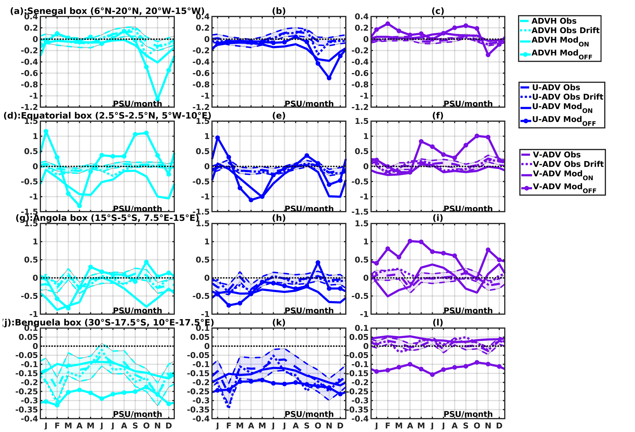
Figure A6 Seasonal cycle of horizontal (cyan), zonal (blue), and meridional (purple) salt advection from observations (dashed line for gridded advection and dotted line for Lagrangian advection) and the model (full line for online and full dotted line for offline) in selected boxes. All others terms are in practical salinity units (psu) per month.