the Creative Commons Attribution 4.0 License.
the Creative Commons Attribution 4.0 License.
 | 21 Apr 2023
An analogues-based forecasting system for Mediterranean marine-litter concentration
In this work, we explore the performance of a statistical forecasting system for marine-litter concentration in the Mediterranean Sea. In particular, we assess the potential skills of a system based on the analogues method. The system uses a historical database of marine-litter concentration simulated by a high-resolution realistic model and is trained to identify meteorological situations in the past that are similar to the forecasted ones. Then, the corresponding marine-litter concentrations of the past analogue days are used to construct the marine-litter concentration forecast. Due to the scarcity of observations, the forecasting system has been validated against a synthetic reality (i.e., the outputs from a marine-litter-modeling system). Different approaches have been tested to refine the system, and the results show that using integral definitions for the similarity function, based on the history of the meteorological situation, improves the system performance. We also find that the system accuracy depends on the domain of application being better for larger regions. Also, the method performs well in capturing the spatial patterns but performs worse in capturing the temporal variability, especially the extreme values. Despite the inherent limitations of using a synthetic reality to validate the system, the results are promising, and the approach has potential to become a suitable cost-effective forecasting method for marine-litter concentration.
- Article
(4845 KB) - Full-text XML
- BibTeX
- EndNote


The ubiquity of the plastic waste pollution in seas and oceans worldwide raises great concern in society and the scientific community, as it poses a significant environmental and socioeconomic threat (UNEP, 2009). In consequence, the analysis of the impacts of marine-litter pollution on marine life and ecosystems has become a hot topic in marine research in recent years (Maximenko et al., 2019; Van Sebille et al., 2020; Lebreton et al., 2019; Lebreton and Andrady, 2019; Soto-Navarro et al., 2021). Marine-litter particles accumulate in both shallow and deep waters and particularly in enclosed basins such as the Mediterranean Sea (Soto-Navarro et al., 2020; Cózar et al., 2015), where the observed concentrations are in the same range as those measured in the great plastic patches formed in the subtropical gyres of the open oceans (Cózar et al., 2015; Law et al., 2014; Van Sebille et al., 2015). Moreover, risk analyses have shown that marine organisms in the Mediterranean basin can be highly impacted by marine-litter pollution (Compa et al., 2019; Soto-Navarro et al., 2021). The starting point to analyze those impacts and to establish suitable mitigation strategies is to understand the spatial distribution and temporal evolution of the marine-litter particles. Unfortunately, to carry on that analysis solely based on observations is not feasible. The large spatial and temporal heterogeneities of the field campaigns, along with the lack of standardized observational protocols, do not allow a synoptic representation of the marine-litter distribution (see Maximenko et al., 2019, for a thorough analysis of the marine-litter-observation problems and proposed improvements). For these reasons, numerical modeling emerges as a fundamental tool for achieving a synoptic description of marine-litter dispersion patterns and as the base for the forecasting systems that would reproduce marine-litter spatial variability and time evolution.
Marine-litter-forecasting systems are usually based on the combination of two different numerical models (Lebreton et al., 2012; Van Sebille et al., 2015; Maximenko et al., 2012). On the one hand, an ocean circulation forecasting system is implemented to provide ocean currents. On the other hand, a Lagrangian model uses those currents to simulate the advection and diffusion of passive particles in the ocean that mimic the evolution of marine litter. In the Mediterranean, several studies using this methodology have been carried out using current fields from high-resolution regional models covering the whole basin (Liubartseva et al., 2018; Macias et al., 2019; Mansui et al., 2015; Soto-Navarro et al., 2020) or specific regions such as the Adriatic, the Tyrrhenian or the Aegean (Politikos et al., 2017; Fossi et al., 2017; Liubartseva et al., 2016; Palatinus et al., 2019). This modeling approach is considered to be the most accurate choice for marine-litter forecasting (Van Sebille et al., 2020), provided the marine-litter inputs are correctly prescribed (Liubartseva et al., 2018; Soto-Navarro et al., 2020).
The downside of developing a forecasting system based on the direct modeling approach is that it involves a high technical complexity and computational cost. In order to overcome these limitations, it might be possible to develop a fast and light forecasting system based on statistical methods. One choice would be the so called statistical downscaling methods (SDMs) which rely on determining statistical relationships between large-scale variables (usually atmospheric patterns) and local variables. They are broadly used in atmospheric modeling to forecast the evolution of local variables within large-scale atmospheric models. The advantage of the SDMs is that the mathematical relationship derived by the model between the local and the large-scale variables is not only valid for the present climate but can also be used to estimate the future evolution of the local variables. In summary, the SDMs provide a simplified static methodology to forecast the evolution of local variables without running complex dynamical models. There are numerous downscaling methodologies based on different statistical properties. Among them, the analogues method (Lorenz, 1969) is the most broadly used due to its simplicity and accuracy (Grouillet et al., 2016). This technique assumes that similar (or analogous) atmospheric patterns over a given region, represented by large-scale atmospheric variables or predictors, lead to similar local meteorological outcomes (or predictands) in a particular location. This assumption provides a simple algorithm to downscale the local occurrence of the variable of interest from a given large-scale atmospheric pattern (see Sect. 2.1 for a detailed description). In general, it has been shown that the analogues method performs as well as other more sophisticated downscaling techniques (Zorita and von Storch, 1999), indicating that it is an efficient alternative to many downscaling problems. Its main advantages are that it is non-parametric (i.e., no assumptions are made about the distribution of the variables used as predictors), non-linear (i.e., it can take into account the non-linearity of the relationships between predictors and predictands), and spatially coherent (i.e., it preserves the spatial covariance structure of the local variables). The analogues method has been satisfactorily applied in the Mediterranean region not only for the downscaling of meteorological or hydrological variables, such as precipitation or river runoff (Grouillet et al., 2016; Wu et al., 2012; Caillouet et al., 2016), but also for the reconstruction of sea surface temperature in the glacial period (Hayes et al., 2005), the assimilation of satellite-derived sea surface height (Lopez-Radcenco et al., 2019) and the projection of complex climatic impact indices such as the fire weather index or the physiological equivalent temperature (Casanueva et al., 2014).
In this study, we explore the feasibility of a marine-litter-concentration forecasting system based on the analogues method. In particular, the surface marine-litter concentration is linked to the atmospheric patterns of a reference period. Then, during the forecasting phase, the forecasted atmospheric situation is compared to that realized during the reference period to identify analogue situations. The marine-litter concentration during those analogue situations is considered to be a good approximation of the marine-litter concentration that will occur during the forecasted date. As this is a new approach that has never been tested before for marine-litter dispersion, the first step was to run several tests to fine-tune the methodology and to characterize its limits in terms of validity. Ideally, the tuning and validation of the method should have been done using in situ observations, but unfortunately, the available marine-litter concentration datasets are too scarce, and this was not possible. Therefore, in this exploratory study, we have used numerically simulated marine-litter concentration fields for the development and validation of the system.
The rest of the paper is organized as follows. In Sect. 2, the statistical method, the datasets used and the different choices tested are introduced. In Sect. 3, the model results are presented and discussed, and finally, some conclusions about the capabilities of this new approach are outlined in Sect. 4.
2.1 The analogues method
The implementation of the analogues method requires two sets of data. First, we need a reference dataset of the variables that describe the atmospheric patterns over the region of study, the so-called predictors (X). The second reference dataset consists of spatial patterns of the variable of interest for the same period for which the predictors are available. In our case, those predictands (Y) would be the marine-litter concentration fields. Once they are defined, the methodology is based on the assumption that, if two predictors are similar (X1∼X2), the corresponding predictands would also be similar (Y1∼Y2). Then, in order to obtain a forecast of the marine-litter concentration for a given date (Yfcst), what we can do is use a forecast of the predictor for the same date (Xfcst). In particular, we look for k analogue dates within the reference period (tan,k) in which the predictor patterns are similar to the forecasted ones (). Then the value of the variable of interest is estimated as a function of the predictands corresponding to the selected analogue dates (). A scheme of the model algorithm is shown in Fig. 1a.
In our case, the predictors used to characterize the atmospheric conditions will be the sea-level pressure (SLP) and the wind speed (U10, V10). These two variables have been successfully used to forecast ocean surface dynamics (Wang et al., 2010; Martínez-Asensio et al., 2016), so it is reasonable to think that they may also be good for forecasting marine-litter concentration, as it is mainly driven by ocean currents. The reference dataset for the atmospheric situation is obtained from an atmospheric reanalysis (see Sect. 2.3). Regarding the reference dataset for the predictand, we use the marine-litter concentration outputs from the modeling system developed by Soto-Navarro et al. (2020) and described in Sect. 2.4.

Figure 1(a) Scheme of the functioning of the analogues method. (b) Example of the JM1 cost function. The vertical red line marks the date forecasted (tfcst – 26 April 2006 in the example). The thin black line is the JM1 cost function for the whole period in the Mediterranean Sea region. Blue dots and vertical dashed lines indicate the analogue dates selected (tan,k; see text for details).
2.2 Algorithm implementation
The first step to implement the analogues method is to define a cost function, JM, that measures the similarity between different meteorological situations. Then, for the forecast day (tfcst), we estimate how close the meteorological situation of that day is to the rest of the days in the reference dataset by computing JM for the whole reference period. Those days with the lowest JM values are selected as the analogue days ({tan,k}; see Fig. 1b for an example). For the definition of JM, the most popular choice is to use the Euclidean distance or root-mean-square-error difference (RMSED; Zorita et al., 1995; Cubasch et al., 1996; Gutiérrez et al., 2013), although other metrics based on different statistics can also be used. Here, we have tested the following four different definitions for the cost function JM:
So, the similarity between meteorological situations is assessed either in terms of the sea-level pressure (SLP – JM1), the 10 m winds (U10, V10 – JM2), a normalized combination of both (JM3) or the cumulated values of JM3 during a period (Δt) before the reference day (JM4). In our case, Δt has been set to 7 d. Note that the horizontal bars indicate spatial averages for JM1 and JM2, while <> in JM3 denotes the temporal mean.
In a second step, we identify the analogue dates as being those with the lowest values of JM. We keep those dates in which JM is lower than the 1 % percentile of all JM. Then the marine-litter concentration maps (C) obtained in the reference dataset for those days are combined to produce the forecast concentration map (Cfcst). In our case, we use the median to reduce the influence of extreme concentration values close to the marine-litter sources as follows:
2.3 Reanalysis data for the atmospheric fields
The period considered for the implementation of the analogues method is 2003–2013, which coincides with the period simulated by the marine-litter dispersion model (as described in the following section). The climatic dataset necessary for the model reference period is based on the ERA5 reanalysis dataset, available at the Copernicus Climate Change Service (C3S) web platform (https://climate.copernicus.eu/climate-reanalysis, last access: 17 May 2021). All the information regarding the ERA5 characteristics can be found on the C3S website.
Two variables have been considered for the characterization of atmospheric patterns forcing the marine-litter dispersion, namely the wind speed at 10 m height (U10, V10) and the sea-level pressure (SLP). Daily mean values of these variables over the Mediterranean Sea were downloaded and processed for the whole period. The spatial resolution of the atmospheric data is 0.25∘ (∼ 25 km), covering the whole Mediterranean basin and the region of the North Atlantic adjacent to the Iberian Peninsula. Figure 2 shows as an example the average SLP for the year 2013 in the selected domain.
2.4 Marine-litter concentration data
The marine-litter concentration data are obtained from the simulations performed by Soto-Navarro et al. (2020), as they are considered to be among the most realistic for the Mediterranean Sea. Due to the relevance of the quality of the marine-litter concentration data, some details on the modeling system are presented below, and more information can be found in Soto-Navarro et al. (2020).
The system is based on the following two components: a regional high-resolution circulation model (RCM) that reproduces the 3D current velocity field in the Mediterranean (NEMOMED36) and a Lagrangian model that simulates the evolution of floating particles (Ichthyop 3.3).
The hydrodynamical model used to simulate the Mediterranean current field is an implementation on the NEMO model, with a spatial resolution of ∘ (∼ 3 km) in a domain that covers the whole Mediterranean. The atmospheric forcing is a dynamical downscaling performed by the ARPEGE-Climate model that uses spectral nudging, namely ARPERA (Herrmann and Somot, 2008). Note that the forcing of NEMOMED36 (ARPERA) is not the same as the one used to characterize the meteorological situations (ERA5). Although both datasets are very similar, they are not exactly the same, thus mimicking the inaccuracies that atmospheric forecasts will inherently have.
The individual-based model (IBM) Ichthyop 3.3 (http://www.ichthyop.org/, last access: 21 June 2019) is used to determine the 3D trajectories of the virtual marine-litter particles from the NEMOMED36 current field. In the coastlines and the domain's boundaries, the configuration of the model is set to “bouncing”, meaning that the particles rebound back to the sea when reaching coastal pixels or the boundary of the domain. Therefore, no beaching scheme is implemented. Following the estimations of Jambeck et al. (2015), a total input of 100 k tonnes of plastic per year into the whole Mediterranean Sea is set in the model. This total amount is distributed by three different types of sources, namely cities, rivers and maritime traffic or shipping lanes according to the ratio %, respectively. The modeling period covers 10 years, between 2003 and 2013. Due to computational limitations, it has been divided in 120 simulations, each one starting on the first day of each month of each year. A total of 41 872 particles are released every month, which, for the complete experiment, makes a total of more than 5 million particles. The initial concentrations at the different source locations are represented in Fig. 3a. The experiments were carried out using particles with positive (floating), neutral and negative (sinking) buoyancy. In this study, only the results for floating marine-litter particles have been used. Soto-Navarro et al. (2020) showed that the dispersion patterns for floating and neutral particles are very similar; hence, the results described below can also be considered valid for neutral particles.
The results of the numerical experiments are processed to produce average marine-litter concentration maps over the Mediterranean basin. These maps are computed by dividing the Mediterranean basin into a regular grid of cells. The average concentration is estimated as the number of particles in each cell divided by the cell surface at each time step. Figure 3b shows the average marine-litter concentration in the Mediterranean for the whole simulated period.
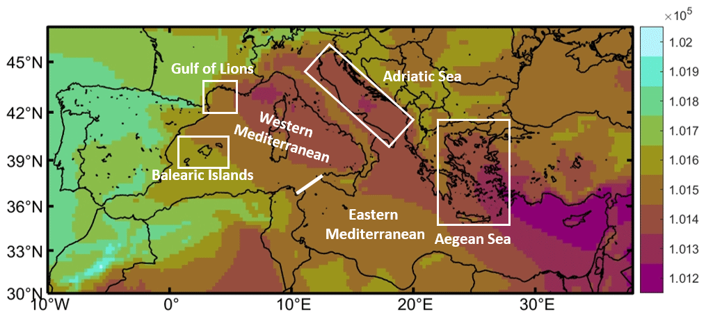
Figure 2Average SLP (in Pa) for the year 2013 in the region, computed from the ERA5 dataset. The red line at the Strait of Sicily marks the boundary between the western and eastern basins. The red rectangles limit the sub-basins of the Balearic Islands, the Gulf of Lions and the Aegean Sea, where specific analyses were carried out.
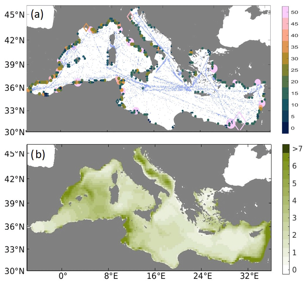
Figure 3(a) Spatial distribution of initial marine-litter concentrations (in kg km−2) for the three simulations. Filled circle points indicate cities, diamonds indicate rivers, and points over the sea indicate the shipping lanes. (b) Average marine-litter concentration of neutral particles (kg km−2) for the period 2003–2013.
2.5 Experiments
As mentioned before, there are no suitable observational datasets to validate the forecasting system. Homogenized datasets covering a long period of time would be required for this task. Although there have been some efforts to develop new databases (Maximenko et al., 2019), to our knowledge, there are no such datasets in the Mediterranean yet. Thus, in order to have a first assessment of the quality of this methodology, we have to use the marine-litter concentration maps from the database as a virtual reality and compare the forecast (Cfcst) with the C in the database for the forecast date (C(tfcst)). We are aware that this may produce overly optimistic results, and this issue will be discussed below.
To define the forecast day, we pick any date from the reference period and forecast the marine litter for that day using all the data available except for that from a week before and after the forecast day to avoid spurious good results due to autocorrelation. This has been repeated for all the days in the reference period (3 650), and several statistical metrics have been computed to assess the skills of the method.
To test if the model shows different skills depending on the domain of application, we have applied the method to the following seven different regions: the whole Mediterranean, the eastern and western basins, the Gulf of Lions, the region around the Balearic Islands, the Adriatic Sea, and the Aegean Sea (see Fig. 2). In each case, the analogue days have been defined using only data on the selected region.
Additionally, we have tested if the skill of the method depends on the timescales of the marine-litter concentration variability. So, in addition to using the marine-litter concentration dataset, we have used two filtered versions of it, separating those processes above and below 15 d (Chi-freq and Clo-freq).
Finally, for completeness, we propose three additional models for the forecasting. First, we forecast the concentration change over 7 d (Δ7 dC). The underlying idea is that the meteorological situation could be a better predictor of the rate of change than of the absolute value (e.g., winds may determine the changes in the concentration rather than the absolute value). The second one is to simply assume 7 d long persistence as the forecasting model (i.e., we assume C(tref)=C(tref-7 d)). This model will tell us whether having a good observational characterization of the marine-litter concentration would be a good predictor of what will be the situation 1 week later. The last one is a combination of the previous two; we add the forecast of the concentration change to the 7 d long persistence (. In other words, we test whether combining a good observational characterization of the marine-litter concentration with an analogues-based forecast of the concentration change can improve the results.
In summary, we have tested four configurations of the model over seven different regions to forecast C, Chi-freq and Clo-freq
2.6 Quality assessment
Several diagnostics are used to characterize the quality of the forecasts in the different experiments. The first one is the root-median-square error (RMEDSE):
We have chosen this parameter instead of the root-mean-square error to reduce the overall impact of outliers linked to very-high-concentration values close to marine-litter sources. Complementarily, we also compute the temporal correlation ρ as follows:
where Cov represents the covariance, and σ represents the standard deviation. Additionally, we compute the RMEDSE ratio (RR), which is defined as the ratio between the RMEDSE of the forecast (Eq. 6) and the RMEDSE computed using all the days in the database, RMEDALL:
The lower the value of RR is, the better the forecast is. Values of RR close to 1 mean that the quality would be the same as when using any random day and that the forecast thus provides no new information. RMEDSE, ρ and RR are computed spatially and/or temporally.
3.1 Time variability
The temporal correlation and the RR of the marine-litter concentration reconstruction using different cost functions and forecasting models are presented in Figs. 4 and 5. The spatial patterns of the correlation are very consistent among the different combinations. The fields are relatively patchy, with the highest values in the eastern basin, close to the Turkish coasts, in the Gulf of Gabes, in the west of Sardinia and towards the north of the Balearic Islands. Conversely, the minimum correlation values are found in the Alboran Sea, the Algerian basin and the Gulf of Lions. The RR maps are very consistent, showing lower values where and when the correlation is higher and values closer to 1 where and when the correlation is lower.
Concerning the different cost functions used to identify the analogue situations, the performances using only SLP (JM1) or only wind (JM2) are very similar. Using both variables, the quality increases slightly (JM3) and becomes significantly better when using the 7 d average (JM4). For model 1 (forecasting the concentration), the averaged correlations using each cost function are 0.24, 0.25, 0.28 and 0.35, while the averaged RR are 0.93, 0.93, 0.90 and 0.86, respectively. The forecasting of the concentration change is worse for all cost functions, with averaged correlation values ranging from 0.08 to 0.19 and RR ranging from 1.00 to 0.98. In light of these results, from now on, we will only consider the results of the analogues-based forecast models that use the cost function JM4 (i.e., the one considering the 7 d averaged differences). Using it for forecasting the marine-litter concentration, we obtain correlation values ranging from 0.20 up to 0.60 depending on the region. When forecasting the marine-litter concentration change, the values range from non-significant to 0.40 (see Fig. 4).
Using 7 d long persistence to forecast the marine-litter concentration (model 3; see Fig. 4), the results largely improve. They show correlations that range from 0.20 in the Alboran Sea and the Gulf of Lions to 0.82 around Cyprus, with an average value of 0.60. The RR reaches values as low as 0.4, with an average value of 0.79. Finally, combining both methodologies in model 4 provides the best results. Combining the 7 d long persistence with the analogues-based forecast of the concentration change increases the forecasting skills. In this case, the averaged correlation is 0.62, and the averaged RR is 0.79.

Figure 4Temporal correlation of the forecasts using different models and cost functions with the reference dataset. Each column corresponds to a different forecasting model: the analogues-based forecast of the concentration (model 1), the analogues-based forecast of the concentration changes over 7 d (model 2), the 7 d long persistence (model 3), and the 7 d long persistence in combination with the forecast of the concentration change over 7 d (model 4). Each row corresponds to the different cost functions used to identify the analogues (see text for details). Note that all panels in the third column are the same, as in model 3 no cost function is used.
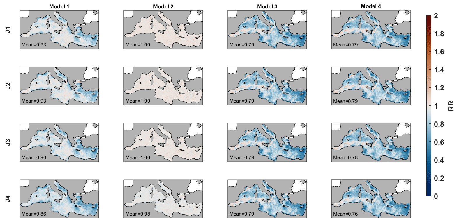
Figure 5Same as Fig. 5 but for the RMEDSE ratio. Values close to 1 (white) indicate that the forecast brings little improvement with respect to using a random day.
For completeness, we also include an example of the concentration time series for the reference and models 1, 3 and 4 for a point where the forecasts perform well (Fig. 6a). It can be seen that model 1 is well correlated with the reference, showing a good chronology of events despite being unable to capture the concentration peaks. During those periods, the analogues-based forecast largely underestimates the reference values. Models 3 and 4 show almost identically good results as far as the persistence is enough to capture most of the variability. The underlying reason for this success is that, at this location, the changes in marine-litter concentration are relatively slower, so assuming persistence can be a good predictor. For comparison, the time series for a point where the models perform poorly are shown in Fig. 6b. In this case, the analogues-based forecast is unable to capture any variability, and it basically produces the mean value. The other two models are able to follow the variability, although in this case, the skills are lower than in the previous case. The reason is that, at this point, the marine-litter concentration varies more rapidly, so assuming the persistence is not as good a predictor as it was in the previous location.
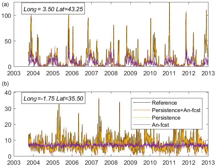
Figure 6Time series of marine-litter concentration (in kg km−2) for (a) a location where the analogues-based forecast works well and (b) a location where it performs worse. The plots show the reference values, the analogues-based forecast, the 7 d long persistence and the 7 d long persistence in combination with the forecast of the concentration change.
3.2 Spatial variability
A complementary view of the performance of the different forecasting models can be obtained by looking at the marine-litter concentration anomalies (i.e., with respect to the temporal mean) on given dates. In Fig. 7, we show the results for a date when the models show good agreement with the reference (spatial correlation values are 0.70, 0.76 and 0.78 for models 1, 3 and 4, respectively). All three models are able to identify the areas of high and low concentrations. Maximum values in the north of the Balearic Islands, the Gulf of Gabes and the south of Italy and minimum values in the Adriatic Sea, the Algerian basin and the easternmost part of the Mediterranean are well captured. The analogues-based forecast (model 1) shows smoother patterns with fewer low extremes. This is in good agreement with what has been seen in the time series in Fig. 6, suggesting that this model presents with difficulties in capturing very high concentration values. Regarding the persistence-based models, for this particular date, they perform very well, capturing not only the large-scale patterns but also the local features. Looking at a date when the performance is lower, something interesting appears. Although the spatial correlation of model 1 is not significant (Fig. 8b), the large-scale features seem to be well captured. However, the small-scale features are clearly not captured, which degrades the spatial correlation. This would also support the previous finding reinforcing the idea that the analogues-based forecast performs better for the large-scale features. In places or dates where or when the small-scale features become dominant, the performance of the model drops.

Figure 7Maps of marine-litter concentration anomalies for a date where the analogues-based forecast performs well. (a) Reference, (b) analogues-based forecast, (c) 7 d long persistence and (d) 7 d long persistence in combination with the forecast of the concentration change over 7 d.
The time series of the spatial correlations and spatial RR at each time step are presented in Fig. 9. The results are similar for the three models forecasting the marine-litter concentration (models 1, 3 and 4). The skills of the forecasts show a high temporal variability, with correlation values ranging from 0.5 to almost 1 and an averaged value of 0.78, 0.81 and 0.84, respectively. For RR, the values range from 0.3 to more than 1, with an average value of 0.76, 0.79 and 0.71, respectively. This diagnostic also confirms that the best model is the one that combines the persistence with the forecast of the concentration change.
3.3 Regional dependence of the forecasting skills
The methodology has also been applied to different domains. That is, the cost function, JM, has been computed in the regions defined in Fig. 2, and the validation has been performed looking only at the marine-litter concentration in those regions. In general, better results are obtained when the analogues-based forecasts are applied to a larger region (see Tables 1 and 2). For instance, the analogues-based forecast (model 1) provides modest results, with correlations of 0.31 and 0.35 and RR of 0.92 and 0.86 for the eastern and western Mediterranean, respectively. At a local scale, the correlation ranges between 0.29 and 0.34, and the RR ranges between 0.80 and 0.94. The analogues-based forecast for the concentration change (model 2) shows lower skills, with correlations below 0.23 and RR above 0.98 in all regions. Both models show better performance when forecasting the low-frequency component than when forecasting the high-frequency one. The correlations of model 1 forecasts in the different regions range between 0.31 and 0.40 for the low-frequency component, while they range between 0.15 and 0.22 for the high-frequency component. Consistent results are found when looking at the RR and model 2 forecasts.
The 7 d long persistence (model 3) is shown to be a good predictor for the full signal and the low-frequency component, but it struggles to capture the high-frequency variability, as expected. Provided that the low-frequency part of the signal is what dominates the marine-litter concentration variability, this model shows good skills for the full signal, with correlations in all regions ranging from 0.55 to 0.64 and RR ranging from 0.75 to 0.82.
The best results for the forecast of the marine-litter concentration are obtained when combining the 7 d long persistence with the analogues-based forecast of the 7 d concentration change (model 4). The averaged temporal correlation is over 0.54 in all regions, reaching a value of 0.65 when applied to the western Mediterranean, while RR is below 0.80 and reaches 0.76 for the whole Mediterranean.
Table 1Regionally averaged temporal correlation of the different forecasting models (M1–M4) applied in different regions (see Fig. 2). The models have been applied to forecast the full signal of marine-litter concentration, the high-frequency component (period < 15 d) and the low-frequency component (period > 15 d).
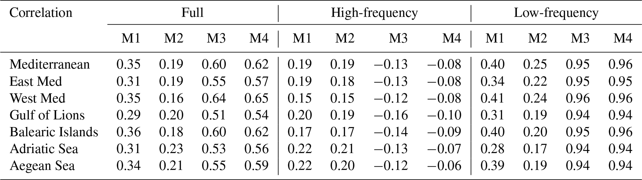
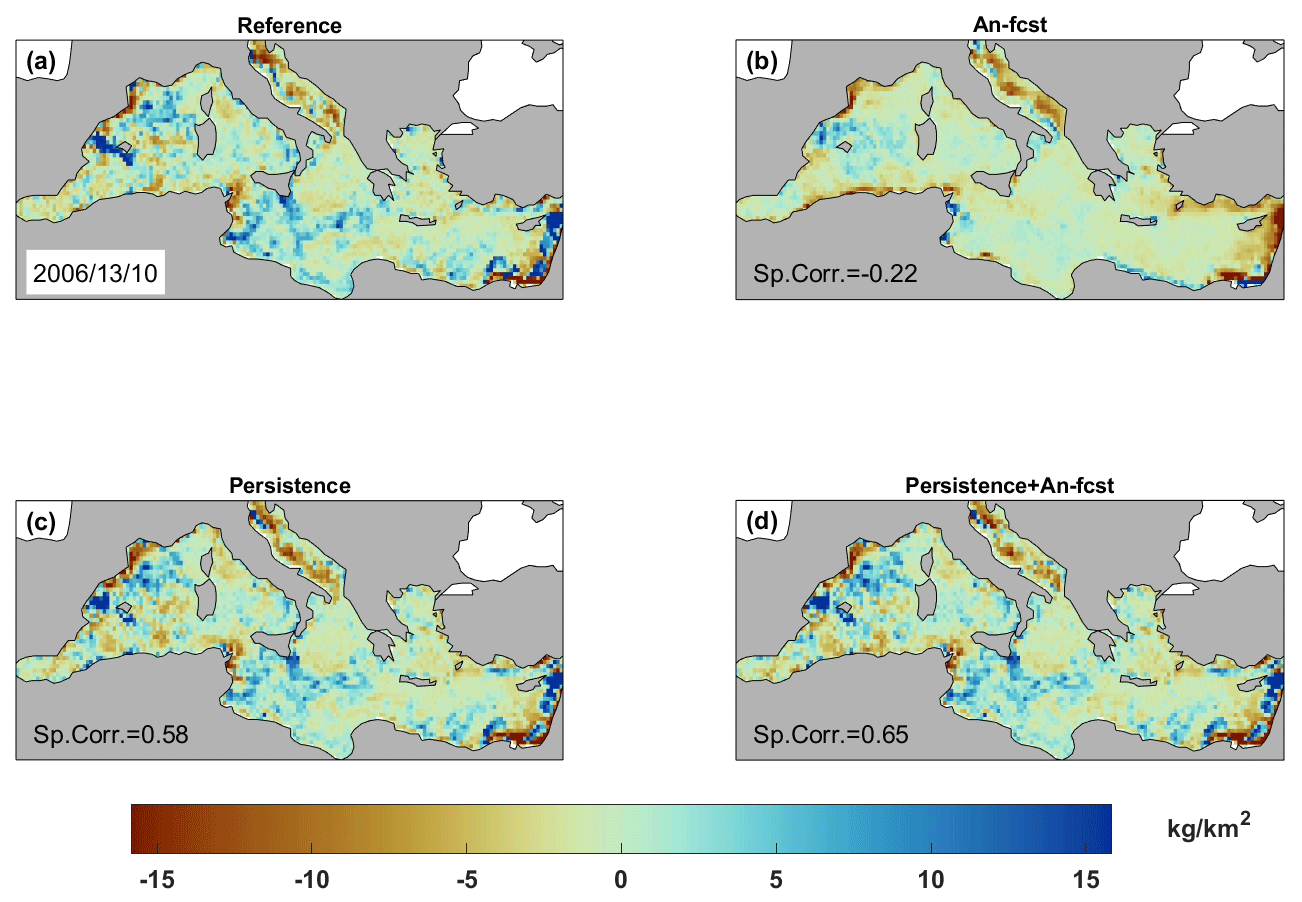
Figure 8Same as Fig. 7 but for a situation where the forecasts perform worse.
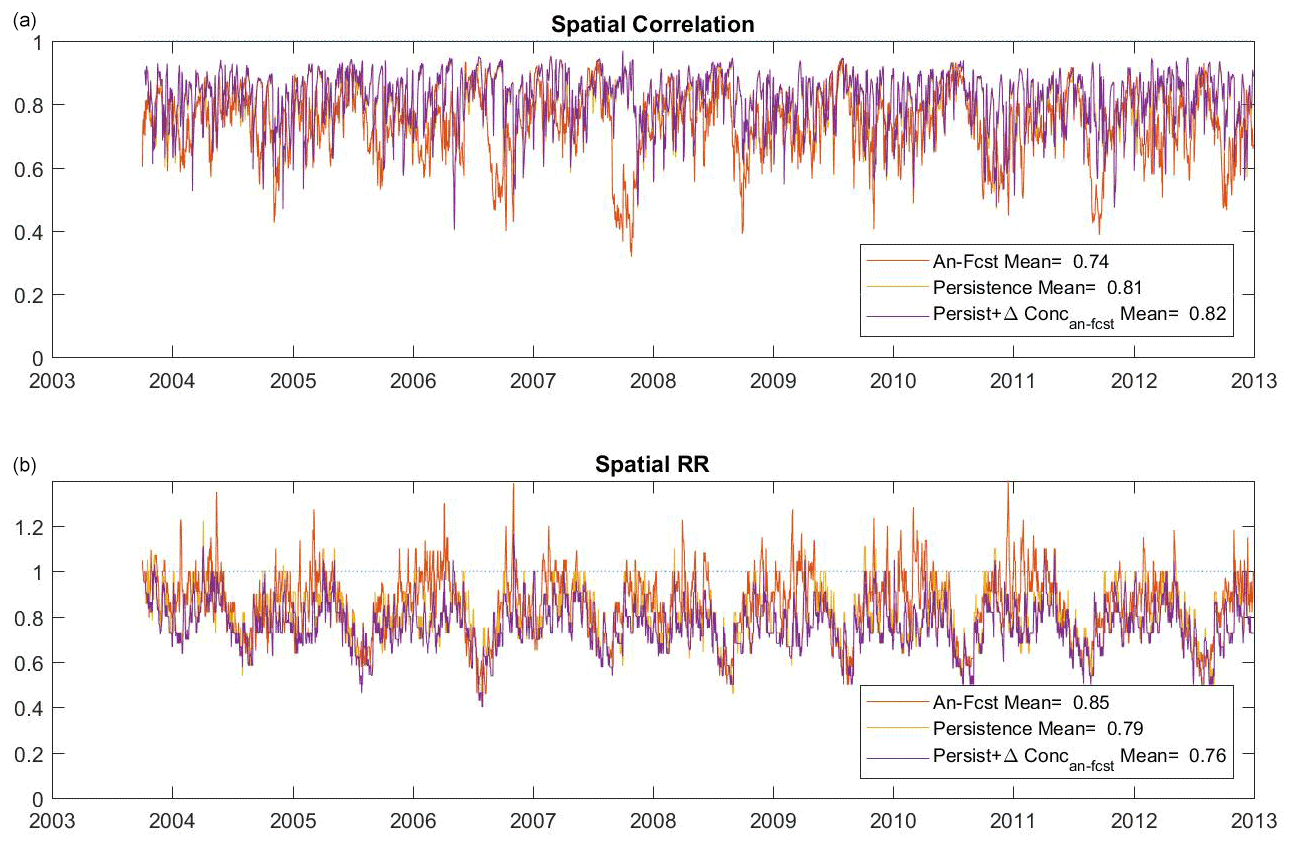
Figure 9Time series of (a) spatial correlation and (b) spatial RR for the analogues-based forecast (model 1), the 7 d long persistence (model 3), and the 7 d long persistence in combination with the forecast of the concentration change (model 4).
The spatial diagnostics have also been computed by applying the models to different domains (Table 3). In this case, the analogues-based forecast of concentration (M1) shows average spatial correlations higher than 0.62 when applied to any region, reaching up to 0.94 in the Aegean Sea. Also, the analogues-based forecast of concentration change (M2) shows significant average correlations, ranging between 0.19 and 0.30. The 7 d long persistence (M3) again shows an improvement in the results, although the combination of the 7 d long persistence and the analogues-based forecast of concentration change (M4) is the best model when applied in any region. The average correlation ranges between 0.67 and 0.96, and RR is lower than 0.83 everywhere.
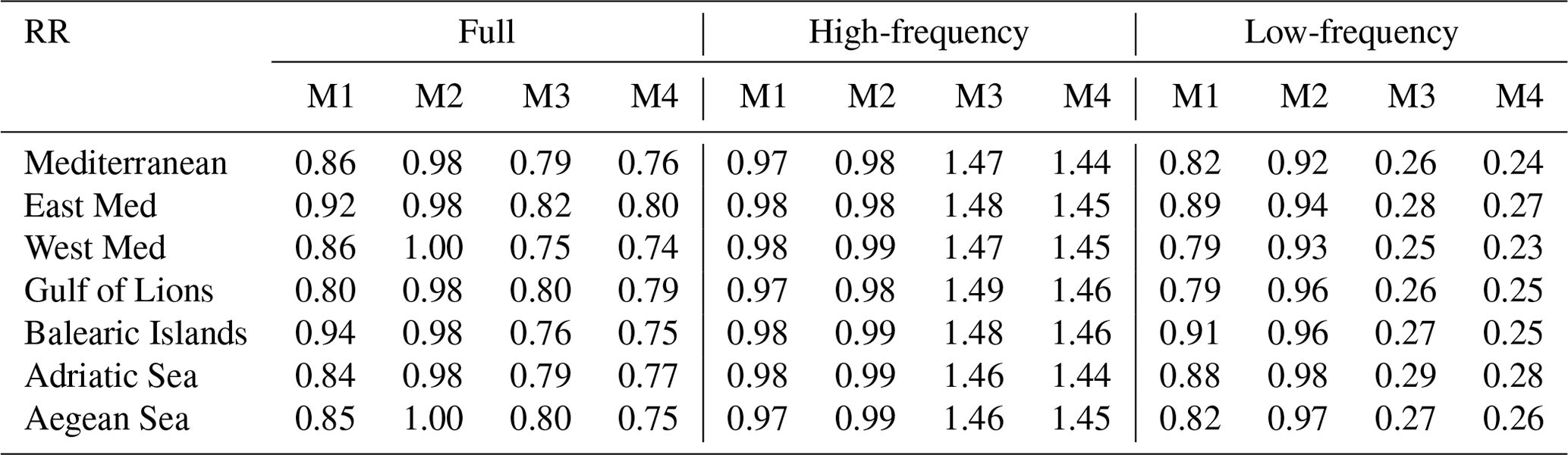
Table 3Temporally averaged regional correlation and RR of the different forecasting models (M1–M4) applied in different regions (see Fig. 2).

It is worth mentioning that we have also tested other options for the cost function, such as using different temporal averages or using correlations as similarity metrics, but no significant differences have been found. Also, we have tried to change the criterion for defining the analogue days. Instead of identifying as analogues those days with JM lower than the 1 % percentile of the whole JM time series, we have used less-restrictive criteria (5 % or 10 %). In both cases, the results worsened.
The analogues-based forecasting technique has been applied to marine-litter concentration for what is, to our knowledge, the first time. It has proven to be very inexpensive and relatively easy to set up, so it is an alternative to direct modeling worthy of being considered. A key step in the set-up is to select a suitable cost function and the best threshold to identify the analogue meteorological situations. In our case, it seems that using integral definitions for the cost function improves the results. In other words, it is better to identify the analogue days based on the history of the meteorological situation. It is probable that using a different averaging time for each domain would allow for an increase in the skills of the analogues-based model. However, this fine tuning is out of the scope of this paper, as there are no suitable observations to validate it, as will be discussed later.
The quality of the analogues-based forecasts depends on the region of application. Our results suggest that the larger the region of application, the better, as we get better results for the whole Mediterranean or for the eastern and western basins than for smaller local areas. A hypothesis for explaining this result is that using the atmospheric situation as a predictor may not be suitable for capturing small-scale features (e.g., those related to ocean currents or the interaction with coastlines). Further tests including other predictors, such as ocean currents, could be done to refine the method.
Another important point is that the method struggles to capture the extreme values, as it produces smooth spatiotemporal patterns of marine-litter concentration. Therefore, in locations or regions where short, intense events or small-scale features dominate the variability, the method performs worse. This is also one of the reasons why the temporal skills (i.e., temporal correlation and RR) are relatively low (see Sect. 3.1). Conversely, if instead of the time variability it is the spatial structures that are aimed at, the method shows a high level of skill in terms of being able to locate relative maxima and minima (see Sect. 3.2).
We have also shown that persistence is a very good predictor almost everywhere. This is because the marine-litter concentration changes relatively slowly (i.e., the system has memory of several days), at least at the spatial scales solved by the reference dataset. This means that, if reliable information was available (e.g., from a monitoring program), this could be used as a first guess regarding the marine-litter concentration several days later. Complementarily, the analogues-based method has also been applied to forecasting concentration change. In this case, the results were significantly poorer in terms of capturing both the time and spatial variability. However, the analogues-based method could be useful for improving the persistence-based forecasts.
Regarding the reliability of the analogues-based forecasts that could be generated from this reference dataset, its quality would directly depend on the accuracy of the reference dataset. In our case, this dataset comes from the outputs of a realistic modeling (Soto-Navarro et al., 2020). However, the model may have some shortcomings, such as its spatial resolution, beaching parameterization or the realism of marine-litter sources. Consequently, the forecasts would be, in the best case, as good as the model outputs are. Therefore, it would have been better to validate the different forecasting models against actual observations. Unfortunately, the lack of observations with a suitable spatial and temporal coverage prevents us from doing this. In the future, it would be worth setting up a monitoring program with sufficient spatial and temporal resolutions that would allow for a comprehensive-enough reference dataset to be generated. This dataset could be used to train the analogues-based forecasting system and to validate other existing systems.
In any case, it is worth noting that the validation of the methodology can be considered to be robust. For that purpose, it is not required that the reference dataset is an accurate representation of the actual marine-litter concentration. Only the statistics of the marine-litter concentration's spatiotemporal evolution have to be reproduced, and in that sense, the model integrates the effects of a realistic atmospheric forcing and a realistic ocean current field. So, it is expected that the statistics of the marine-litter concentration field are realistic enough. This extent should also be confirmed by a comprehensive observational dataset, at least in certain regions.
In conclusion, the analogues-based model presented here has potential to become a suitable, cost-effective forecasting method for marine-litter concentration. It could be easily implemented in any region of the world where a realistic reference dataset is available. In those regions where the large-scale marine-litter concentration patterns dominate the variability, the method will probably work better than in regions where the variability is dominated by small-scale structures.
The code and data required to implement the model described in the paper and to reproduce the results can be publicly accessed at Jordà and Soto-Navarro (2022). Additionally, the atmospheric fields can be downloaded from the Copernicus portal (https://climate.copernicus.eu/climate-reanalysis, Hersbach et al., 2021).
Both authors (GJ and JSN) contributed equally to the design of the study, the coding of the modeling system, the performance of the simulations, the analysis of the results, and the preparation and revision of the paper.
The contact author has declared that neither of the authors has any competing interests.
Publisher’s note: Copernicus Publications remains neutral with regard to jurisdictional claims in published maps and institutional affiliations.
We acknowledge the Junta de Andalucía-funded Origen y evolución de la basura marina en la costa andaluza (OBAMARAN; reference no. Proy_Exel_00344). The authors also thank Mr. Paul Dupin for his help in the first steps of the model development.
This research has been supported by the European Regional Development Fund, Interreg (grant no. 4MED17_3.2_M123_027). We also received funding from the EU-Interreg MPAs Plastic Busters project: preserving biodiversity from plastics in Mediterranean Marine Protected Areas,
co-financed by the European Regional Development Fund (grant agreement no.
4MED17_3.2_M123_027).
The publication fee was supported by the CSIC Open Access Publication Support Initiative through its Unit of Information Resources for Research (URICI).
This paper was edited by Erik van Sebille and reviewed by Andres Cozar and one anonymous referee.
Caillouet, L., Vidal, J. P., Sauquet, E., and Graff, B.: Probabilistic precipitation and temperature downscaling of the Twentieth Century Reanalysis over France, Clim. Past, 12, 635–662, https://doi.org/10.5194/cp-12-635-2016, 2016.
Casanueva, A., Frías, M. D., Herrera, S., San-Martín, D., Zaninovic, K., and Gutiérrez, J. M.: Statistical downscaling of climate impact indices: testing the direct approach, Climatic Change, 127, 547–560, https://doi.org/10.1007/s10584-014-1270-5, 2014.
Compa, M., Alomar, C., Wilcox, C., van Sebille, E., Lebreton, L., Hardesty, B. D., and Deudero, S.: Risk assessment of plastic pollution on marine diversity in the Mediterranean Sea, Sci. Total Environ., 678, 188–196, https://doi.org/10.1016/j.scitotenv.2019.04.355, 2019.
Cózar, A., Sanz-Martín, M., Martí, E., González-Gordillo, J. I., Ubeda, B., Á.gálvez, J., Irigoien, X., and Duarte, C. M.: Plastic accumulation in the mediterranean sea, PLoS One, 10, 1–12, https://doi.org/10.1371/journal.pone.0121762, 2015.
Cubasch, U., Von Storch, H., Waszkewitz, J., and Zorita, E.: Estimates of climate change in Southern Europe derived from dynamical climate model output, Clim. Res., 7, 129–149, https://doi.org/10.3354/cr007129, 1996.
Fossi, M. C., Romeo, T., Baini, M., Panti, C., Marsili, L., Campani, T., Canese, S., Galgani, F., Druon, J.-N., Airoldi, S., Taddei, S., Fattorini, M., Brandini, C., and Lapucci, C.: Plastic Debris Occurrence, Convergence Areas and Fin Whales Feeding Ground in the Mediterranean Marine Protected Area Pelagos Sanctuary: A Modeling Approach, Front. Mar. Sci., 4, 1–15, https://doi.org/10.3389/fmars.2017.00167, 2017.
Grouillet, B., Ruelland, D., Ayar, P. V., and Vrac, M.: Sensitivity analysis of runoff modeling to statistical downscaling models in the western Mediterranean, Hydrol. Earth Syst. Sci., 20, 1031–1047, https://doi.org/10.5194/hess-20-1031-2016, 2016.
Gutiérrez, J. M., San-Martín, D., Brands, S., Manzanas, R., and Herrera, S.: Reassessing statistical downscaling techniques for their robust application under climate change conditions, J. Clim., 26, 171–188, https://doi.org/10.1175/JCLI-D-11-00687.1, 2013.
Hayes, A., Kucera, M., Kallel, N., Sbaffi, L., and Rohling, E. J.: Glacial Mediterranean sea surface temperatures based on planktonic foraminiferal assemblages, Quaternary Sci. Rev., 24, 999–1016, https://doi.org/10.1016/j.quascirev.2004.02.018, 2005.
Herrmann, M. J. and Somot, S.: Relevance of ERA40 dynamical downscaling for modeling deep convection in the Mediterranean Sea, Geophys. Res. Lett., 35, 1–5, https://doi.org/10.1029/2007GL032442, 2008.
Hersbach, H., Bell, B., Berrisford, P., et al.: The ERA5 global reanalysis, Q. J. R. Meteorol. Soc., 146, 1999–2049, https://doi.org/10.1002/qj.3803, 2020 (data available at https://climate.copernicus.eu/climate-reanalysis, last access: 17 May 2021).
Jambeck, J. R., Geyer, R., Wilcox, C., Siegler, T. R., Perryman, M., Andrady, A., Narayan, R., and Law, K. L.: Plastic waste inputs from land into the ocean, Science, 347, 768–771, https://doi.org/10.1126/science.1260352, 2015.
Jordà, G. and Soto-Navarro, J.: An analogue based forecasting system for Mediterranean marine litter concentration – Code and simulations dataset, Zenodo [code and data set], https://doi.org/10.5281/zenodo.7104402, 2022.
Law, K. L., Morét-Ferguson, S. E., Goodwin, D. S., Zettler, E. R., Deforce, E., Kukulka, T., and Proskurowski, G.: Distribution of surface plastic debris in the eastern pacific ocean from an 11-year data set, Environ. Sci. Technol., 48, 4732–4738, https://doi.org/10.1021/es4053076, 2014.
Lebreton, L. and Andrady, A.: Future scenarios of global plastic waste generation and disposal, Palgrave Commun., 5, 1–11, https://doi.org/10.1057/s41599-018-0212-7, 2019.
Lebreton, L., Egger, M., and Slat, B.: A global mass budget for positively buoyant macroplastic debris in the ocean, Sci. Rep., 9, 1–10, https://doi.org/10.1038/s41598-019-49413-5, 2019.
Lebreton, L. C. M., Greer, S. D., and Borrero, J. C.: Numerical modelling of floating debris in the world's oceans, Mar. Pollut. Bull., 64, 653–661, https://doi.org/10.1016/j.marpolbul.2011.10.027, 2012.
Liubartseva, S., Coppini, G., Lecci, R., and Creti, S.: Regional approach to modeling the transport of floating plastic debris in the Adriatic Sea, Mar. Pollut. Bull., 103, 115–127, https://doi.org/10.1016/j.marpolbul.2015.12.031, 2016.
Liubartseva, S., Coppini, G., Lecci, R., and Clementi, E.: Tracking plastics in the Mediterranean: 2D Lagrangian model, Mar. Pollut. Bull., 129, 151–162, https://doi.org/10.1016/j.marpolbul.2018.02.019, 2018.
Lopez-Radcenco, M., Pascual, A., Gomez-Navarro, L., Aissa-El-Bey, A., Chapron, B., and Fablet, R.: Analog Data Assimilation of Along-Track Nadir and Wide-Swath SWOT Altimetry Observations in the Western Mediterranean Sea, IEEE J. Sel. Top. Appl. Earth Obs. Remote Sens., 12, 2530–2540, https://doi.org/10.1109/JSTARS.2019.2903941, 2019.
Lorenz, E. N.: Atmospheric Predictability as Revealed by Naturally Occurring Analogues, J. Atmos. Sci., 26, 636–646, https://doi.org/10.1175/1520-0469(1969)26<636:APARBN>2.0.CO;2, 1969.
Macias, D., Cózar, A., Garcia-Gorriz, E., González-Fernández, D., and Stips, A.: Surface water circulation develops seasonally changing patterns of floating litter accumulation in the Mediterranean Sea. A modelling approach, Mar. Pollut. Bull., 149, 110619, https://doi.org/10.1016/j.marpolbul.2019.110619, 2019.
Mansui, J., Molcard, A., and Ourmières, Y.: Modelling the transport and accumulation of floating marine debris in the Mediterranean basin, Mar. Pollut. Bull., 91, 249–257, https://doi.org/10.1016/j.marpolbul.2014.11.037, 2015.
Martínez-Asensio, A., Marcos, M., Tsimplis, M. N., Jordà, G., Feng, X., and Gomis, D.: On the ability of statistical wind-wave models to capture the variability and long-term trends of the North Atlantic winter wave climate, Ocean Model., 103, 177–189, https://doi.org/10.1016/j.ocemod.2016.02.006, 2016.
Maximenko, N., Hafner, J., and Niiler, P.: Pathways of marine debris derived from trajectories of Lagrangian drifters, Mar. Pollut. Bull., 65, 51–62, https://doi.org/10.1016/j.marpolbul.2011.04.016, 2012.
Maximenko, N., Corradi, P., Law, K. L., Van Sebille, E., Garaba, S. P., Lampitt, R. S., Galgani, F., Martinez-Vicente, V., Goddijn-Murphy, L., Veiga, J. M., Thompson, R. C., Maes, C., Moller, D., Löscher, C. R., Addamo, A. M., Lamson, M. R., Centurioni, L. R., Posth, N. R., Lumpkin, R., Vinci, M., Martins, A. M., Pieper, C. D., Isobe, A., Hanke, G., Edwards, M., Chubarenko, I. P., Rodriguez, E., Aliani, S., Arias, M., Asner, G. P., Brosich, A., Carlton, J. T., Chao, Y., Cook, A.-M., Cundy, A. B., Galloway, T. S., Giorgetti, A., Goni, G. J., Guichoux, Y., Haram, L. E., Hardesty, B. D., Holdsworth, N., Lebreton, L., Leslie, H. A., Macadam-Somer, I., Mace, T., Manuel, M., Marsh, R., Martinez, E., Mayor, D. J., Le Moigne, M., Molina Jack, M. E., Mowlem, M. C., Obbard, R. W., Pabortsava, K., Robberson, B., Rotaru, A.-E., Ruiz, G. M., Spedicato, M. T., Thiel, M., Turra, A., and Wilcox, C.: Toward the Integrated Marine Debris Observing System, Front. Mar. Sci., 6, 447, https://doi.org/10.3389/fmars.2019.00447, 2019.
Palatinus, A., Kovač Viršek, M., Robič, U., Grego, M., Bajt, O., Šiljić, J., Suaria, G., Liubartseva, S., Coppini, G., and Peterlin, M.: Marine litter in the Croatian part of the middle Adriatic Sea: Simultaneous assessment of floating and seabed macro and micro litter abundance and composition, Mar. Pollut. Bull., 139, 427–439, https://doi.org/10.1016/j.marpolbul.2018.12.038, 2019.
Politikos, D. V., Ioakeimidis, C., Papatheodorou, G., and Tsiaras, K.: Modeling the Fate and Distribution of Floating Litter Particles in the Aegean Sea (E. Mediterranean), Front. Mar. Sci., 4, 1–18, https://doi.org/10.3389/fmars.2017.00191, 2017.
Soto-Navarro, J., Jordà, G., Deudero, S., Alomar, C., Amores, Á., and Compa, M.: 3D hotspots of marine litter in the Mediterranean: A modeling study, Mar. Pollut. Bull., 155, 111159, https://doi.org/10.1016/j.marpolbul.2020.111159, 2020.
Soto-Navarro, J., Jordá, G., Compa, M., Alomar, C., Fossi, M. C., and Deudero, S.: Impact of the marine litter pollution on the Mediterranean biodiversity: A risk assessment study with focus on the marine protected areas, Mar. Pollut. Bull., 165, 112169, https://doi.org/10.1016/j.marpolbul.2021.112169, 2021.
UNEP: Matine Litter, A Global Chanllenge, UNEP, Nairobi, 232 pp., ISBN 978-92-807-3029-6, 2009.
Van Sebille, E., Chris, W., Laurent, L., Nikolai, M., Britta Denise, H., Jan, A. van F., Marcus, E., David, S., Francois, G., and Kara Lavender, L.: A global inventory of small floating plastic debris, Environ. Res. Lett., 10, 124006, https://doi.org/10.1088/1748-9326/10/12/124006, 2015.
Van Sebille, E., Aliani, S., Law, K. L., Maximenko, N., Alsina, J. M., Bagaev, A., Bergmann, M., Chapron, B., Chubarenko, I., Cózar, A., Delandmeter, P., Egger, M., Fox-Kemper, B., Garaba, S. P., Goddijn-Murphy, L., Hardesty, B. D., Hoffman, M. J., Isobe, A., Jongedijk, C. E., Kaandorp, M. L. A., Khatmullina, L., Koelmans, A. A., Kukulka, T., Laufkötter, C., Lebreton, L., Lobelle, D., Maes, C., Martinez-Vicente, V., Morales Maqueda, M. A., Poulain-Zarcos, M., Rodríguez, E., Ryan, P. G., Shanks, A. L., Shim, W. J., Suaria, G., Thiel, M., Van Den Bremer, T. S., and Wichmann, D.: The physical oceanography of the transport of floating marine debris, Environ. Res. Lett., 15, 023003, https://doi.org/10.1088/1748-9326/ab6d7d, 2020.
Wang, X. L., Swail, V. R., and Cox, A.: Dynamical versus statistical downscaling methods for ocean wave heights, Int. J. Climatol., 30, 317–332, https://doi.org/10.1002/joc.1899, 2010.
Wu, W., Liu, Y., Ge, M., Rostkier-Edelstein, D., Descombes, G., Kunin, P., Warner, T., Swerdlin, S., Givati, A., Hopson, T., and Yates, D.: Statistical downscaling of climate forecast system seasonal predictions for the Southeastern Mediterranean, Atmos. Res., 118, 346–356, https://doi.org/10.1016/j.atmosres.2012.07.019, 2012.
Zorita, E. and von Storch, H.: The Analog Method as a Simple Statistical Downscaling Technique: Comparison with More Complicated Methods, J. Clim., 12, 2474–2489, https://doi.org/10.1175/1520-0442(1999)012<2474:TAMAAS>2.0.CO;2, 1999.
Zorita, E., Hughes, J. P., Lettermaier, D. P., and von Storch, H.: Stochastic Characterization of Regional Circulation Patterns for Climate Model Diagnosis and Estimation of Local Precipitation, J. Clim., 8, 1023–1042, 1995.