Multiple mechanisms for chlorophyll a concentration variations in coastal upwelling regions: a case study east of Hainan Island in the South China Sea

Using satellite observations from 2003 to 2020 and cruise observations from 2019 and 2021, this study reveals an unexpected minor role of upwelling in seasonal and interannual variations in chlorophyll a (Chl a) concentrations in the coastal upwelling region east of Hainan Island (UEH) in the northwestern South China Sea (NWSCS). The results show strong seasonal and interannual variability in the Chl a concentration in the core upwelling area of the UEH. Different from the strongest upwelling in summer, the Chl a concentration in the UEH area reaches a maximum of 1.18 mg m⁻³ in autumn and winter, with a minimum value of 0.74 mg m⁻³ in summer. The Chl a concentration in summer increases to as high as 1.0 mg m⁻³ with weak upwelling, whereas the maximum Chl a concentration in October increases to 2.5 mg m⁻³. The analysis of environmental factors shows that, compared to the limited effects of upwelling, the along-shelf coastal current from the northern shelf and the increased precipitation are crucially important to the Chl a concentration variation in the study area. These results provide new insights for predicting marine productivity in upwelling areas, i.e., multiple mechanisms, especially horizontal advection, should be considered in addition to the upwelling process.

1 Introduction

The oceanic area with coastal upwelling is generally characterized by high productivity; it occupies only 1 % of the total area of the ocean but provides more than 50 % of the total marine fish harvest (Barua, 2005). High levels of biological productivity strongly influence atmosphere–ocean carbon recycling (Mcgregor et al., 2007; Xu et al., 2020). Therefore, revealing the variation in chlorophyll a (Chl a) in coastal upwelling areas is important to the overall health of the marine ecosystem and climate.

The upward movement of seawater may carry nutrients from the lower layer and support a high surface Chl a concentration. Thus, the variability in Chl a concentrations in coastal upwelling regions is proposed to be associated with that of upwelling (Jing et al., 2009). Alongshore winds, positive wind curl, tidal mixing, and topography may affect upwelling processes (Hu and Wang, 2016). In contrast, other oceanic and atmospheric processes, such as mesoscale eddies, sub-mesoscale fronts, precipitation, and typhoon processes, can also induce Chl a increments (Aoki et al., 2019; Cape et al., 2019; Li et al., 2021a, b).

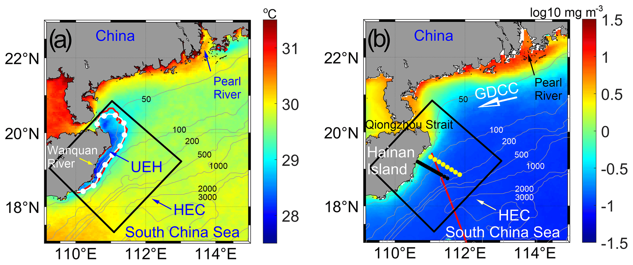
Figure 1 Study area (black square) and sampling sites. (a) Climatological (June–August) sea surface temperature (SST) and (b) Chl a concentration during 2003–2020. In (a), the dotted white curve is the SST front for June–August; the red curve is the 29^∘ isotherm. In (b), the dots are the observation sites for the cruise during 14–15 July 2021 (black) and 2–3 October 2019 (yellow), and the red curve is the altimeter satellite ground track (Track 114). The unit of the numbers on the isobaths is meters.

The coastal upwelling east of Hainan Island (UEH) is part of the seasonal upwelling in the northwestern South China Sea (NWSCS). As shown in Fig. 1, the isobaths in the shelf are parallel to the continental coastline. The width of the continental shelf is approximately 100 km. Outside of the continental shelf, there is a steep slope linking the shelf to the South China Sea (SCS) basin. The circulation in the coastal area east of Hainan Island (HEC) is controlled by the East Asian monsoon system. In summer, the coastal current travels northeastward on the shelf influenced by the southwesterly monsoon, whereas in winter, the current flows southwestward (Ding et al., 2018; Jing et al., 2015). According to the Ekman transport theory, the along-shelf wind induces cross-shelf transport of the surface water and thus causes coastal upwelling along the coastline in summer. The UEH generally begins in April, becomes strongest in July and August, and remains until September (Xie et al., 2012). The UEH is located in coastal shallow water less than 100 m deep (Jing et al., 2015). Wind-stress-curl-induced Ekman pumping is considered to be another crucial factor for UEH generation (Xu et al., 2020). In addition, the strong northeastward current along the shelf could cause strong stratification towards the coast and thus enhance upwelling (Su et al., 2013).

The variation in primary production in the HEC has been variously reported. Deng et al. (1995) reported that phytoplankton achieved a maximum value in a strong period of UEH. Jing et al. (2011) found a higher Chl a concentration in summer 1998, as the offshore Ekman transport was the strongest. Southwesterly monsoon-induced coastal upwelling is suggested to be the major mechanism for the relatively high summertime phytoplankton biomass and primary production (Liu et al., 2013; Song et al., 2012). Moreover, Hu et al. (2021) found that eddy processes could strengthen phytoplankton blooms in the HEC. The variation in the basin circulation may also affect the UEH (Su et al., 2013; Wang et al., 2006). However, Ning et al. (2004) reported poor nutrients, low Chl a, and weak primary production in summer in the HEC. Shi et al. (2021) found that the largest Chl a increase in the HEC occurs in May when upwelling is weak. Li et al. (2021a) further showed that the maximum Chl a concentration year-round exhibits a double peak in March and October.

The results of previous studies indicate that upwelling may not be the most significant factor affecting primary productivity in the HEC (Li et al., 2021a; Ning et al., 2004). The mechanism driving the variation in primary productivity in the HEC thus needs further investigation.

The objective of this study is to reveal the role of upwelling in the spatial and temporal variations in Chl a concentrations in the HEC area based on multi-sensor satellite observations and in situ cruise observations. The article is organized as follows. Section 2 describes the materials and methods, including the algorithms used for retrieval of the total suspended sediment (TSS) and sea surface temperature (SST) from satellite observations. Section 3 presents the results and variations in environmental factors and an analysis of the spatial and temporal variations in the Chl a concentration in the study area. Section 4 discusses the role of typhoons, coastal currents, El Niño–Southern Oscillation (ENSO) events, and precipitation in the Chl a concentration. Section 5 presents the conclusions.

2 Materials and methods

2.1 Study area and upwelling area

The study area (enclosed by the black square in Fig. 1) covers the UEH area off the northeastern coast of Hainan Island. It is adjacent to the narrow Qiongzhou Strait in the west and adjoins the wide continental shelf of the NWSCS in the east. The Wanquan River flowing through the east of Hainan Island is the third largest river on Hainan Island. The East Asian monsoon prevails in the HEC, and the UEH appears along the coast in summer (Lin et al., 2016). In fall and winter, a southwestward current flows along the coast on the whole shelf (Ding et al., 2018; Li et al., 2016). The nutrients in the Pearl River runoff can be transported to the HEC area by the Guangdong Coastal Current (GDCC). The thermal fronts stretch along the continental shelf (dotted white curve in Fig. 1a) and are accompanied by relatively high Chl a concentrations in HEC (Fig. 1b).

2.2 Satellite observations and retrieval

The monthly ocean color elements (Kd490, Rrs645, Chl a, SST, and photosynthetically active radiation (PAR)) were obtained by moderate-resolution imaging spectroradiometer (MODIS) instruments on board the Terra and Aqua satellites. The dataset from 2003 to 2020 is a level-3 product with a spatial resolution of 4 km. The data from the two platforms were merged to improve the coverage of the Chl a concentration (Li et al., 2021b). The TSS concentration was estimated from the Rrs645 product as follows (Li et al., 2021b):

$$\begin{array}{}\text{(1)}& C_{\mathrm{TSS}}=\mathrm{0.6455}+\mathrm{1455.7}\times \text{Rrs}\mathrm{645}.\end{array}$$

The euphotic depth retrieval from the Kd490 product was conducted as follows (Zhao et al., 2013):

$$\begin{array}{}\text{(2)}& Z_{\mathrm{eu}}=\mathrm{0.28}+{\displaystyle \frac{\mathrm{395.92}\times \mathrm{0.0092}}{\mathrm{0.0092}+\text{Kd}\mathrm{490}}}.\end{array}$$

The surface thermal front was estimated using the SST gradient. The SST gradient was calculated using the zonal and meridional components (GSST_x, GSST_y) as follows:

$$\begin{array}{}\text{(3)}& \text{GSST}=\sqrt{{\left({\text{GSST}}_x\right)}^{\mathrm{2}}+{\left({\text{GSST}}_y\right)}^{\mathrm{2}}},\end{array}$$

where GSST${}_{x_i}=\left(\frac{{\text{SST}}_{i+\mathrm{1}}-{\text{SST}}_{i-\mathrm{1}}}{x_{i+\mathrm{1}}-x_{i-\mathrm{1}}}\right)$ (^∘C km⁻¹), and ($x_{i+\mathrm{1}}-x_{i-\mathrm{1}})$ is equal to twice the spatial resolution.

The sea surface wind (SSW) at 10 m above the sea surface, with a spatial resolution of 0.25^∘, was obtained from the Copernicus Marine Service (CMEMS; Hersbach et al., 2018). The wind data are a subset from the fifth-generation European Centre for Medium-Range Weather Forecasts (ECMWF) atmospheric reanalysis of the global climate covering the period from January 1950 to present. The data from 2002 to 2020 used in this study were a monthly product.

A cross-shelf and along-shelf coordinate system for the SSW vector is given by

$$\begin{array}{}\text{(4)}& {\displaystyle }{u}_{\mathrm{along}}=u\text{cos}\mathit{\theta }-v\sin \mathit{\theta },\text{(5)}& {\displaystyle }{v}_{\mathrm{cross}}=u\sin \mathit{\theta }+v\cos \mathit{\theta },\end{array}$$

where the cross-shelf wind, v_cross, is seaward positive; the along-shelf wind, ualong, is northward parallel to the coastline; θ is the angle between the shoreline and the north direction (25^∘ in this study); and (u, v) are the east and north components of the SSW.

The wind stress is determined as

$$\begin{array}{}\text{(6)}& \mathit{\tau }={\mathit{\rho }}_{\mathrm{a}}{C}_{\mathrm{D}}U\left|U\right|,\end{array}$$

where ρ_a, C_D, and U are air density, drag coefficient, and sea surface wind; ρ_a=1.29 kg m⁻³; $C_{\text{D}}=(\mathrm{0.75}+\mathrm{0.067}U)\times {\mathrm{10}}^{-\mathrm{3}}$ (Garratt, 1977). Moreover, wind stress curl is obtained by ∇×τ.

The monthly sea surface salinity (SSS) data from 2018 to 2020, with a spatial resolution of 0.25^∘, were obtained from the CMEMS.

The daily rainfall rate during 2003–2020 was obtained from the multi-satellite precipitation analysis dataset of the Tropical Rainfall Measuring Mission (TRMM). The monthly data, with a spatial resolution of 0.25^∘, were calculated from the daily global rainfall data.

The satellite altimeter along-track sea level anomaly (SLA) data from 2003 to 2020 were obtained from the CMEMS. The Jason-1, Jason-2, and Jason-3 satellites repeat their ground tracks every 9.9 d. Their sampling frequency is 1 Hz, and their spatial resolution is approximately 7 km. The five-point moving average was applied to the along-track SLA data to filter out the small-scale ocean processes. As the coastline is almost perpendicular to ground track 114 of the altimeter satellites (Fig. 1b), the along-shelf geostrophic current was estimated from the along-track SLA data as follows:

$$\begin{array}{}\text{(7)}& u={\displaystyle \frac{g}{f}}{\displaystyle \frac{\partial \mathit{\eta }}{\partial y}},\end{array}$$

where g is the acceleration due to gravity, f is the Coriolis parameter, and η is the SLA.

The typhoon track data were downloaded from the Tropical Cyclone Data Center of the China Meteorological Administration (CMA). The dataset contains 6-hourly tracks and intensity analyses of typhoons that occurred in the western North Pacific from 2003 to 2020.

2.3 Shipboard sections

Two shipboard sections were investigated during 2–3 October 2019 and 14–15 July 2021 (yellow and black points in Fig. 1b). At each station, the temperature, salinity, and fluorescence profiles were collected using a Sea-Bird 911plus conductivity–temperature–depth (CTD) system. The Chl a data from the fluorescence sensor of the CTD were not calibrated, and the signals of interest were clear.

2.4 Mapping the upwelling

The thermal fronts (Fig. 1a) of the climatological SST in summer stretched along the 29 ^∘C isotherm. Thus, we defined the upwelling domain, i.e., core upwelling, as the area where the SST was lower than 29 ^∘C in the summer. The time series of the core upwelling area was calculated for each year during 2003–2020. Then the time series of the Chl a concentration in the core upwelling area for each year was obtained.

The upwelling index (UI) based on the wind stress is as follows:

$$\begin{array}{}\text{(8)}& M_x=-{\displaystyle \frac{{\mathit{\tau }}_y}{f\mathit{\rho }}},\end{array}$$

where ρ=1025 kg m⁻³ is the water density, f is the Coriolis parameter, τ_y is the along-shelf wind stress, and M_x is the cross-transport.

2.5 Empirical orthogonal function

Empirical orthogonal function (EOF) is a useful tool and is widely applied to reduce the dimensionality of climate data (North et al., 1982). EOF analysis is used to determine the dominant patterns of Chl a in the study area. The Chl a data are prepared as an anomaly in the form of matrix, X. Decomposition is applied by $B\cdot E=\mathbf{X}$. EOF modes (i.e., E, spatial patterns) and their corresponding principal components (i.e., B, temporal coefficients) could be obtained by decomposition of the anomaly matrix. The EOF patterns and the principal components are independent.

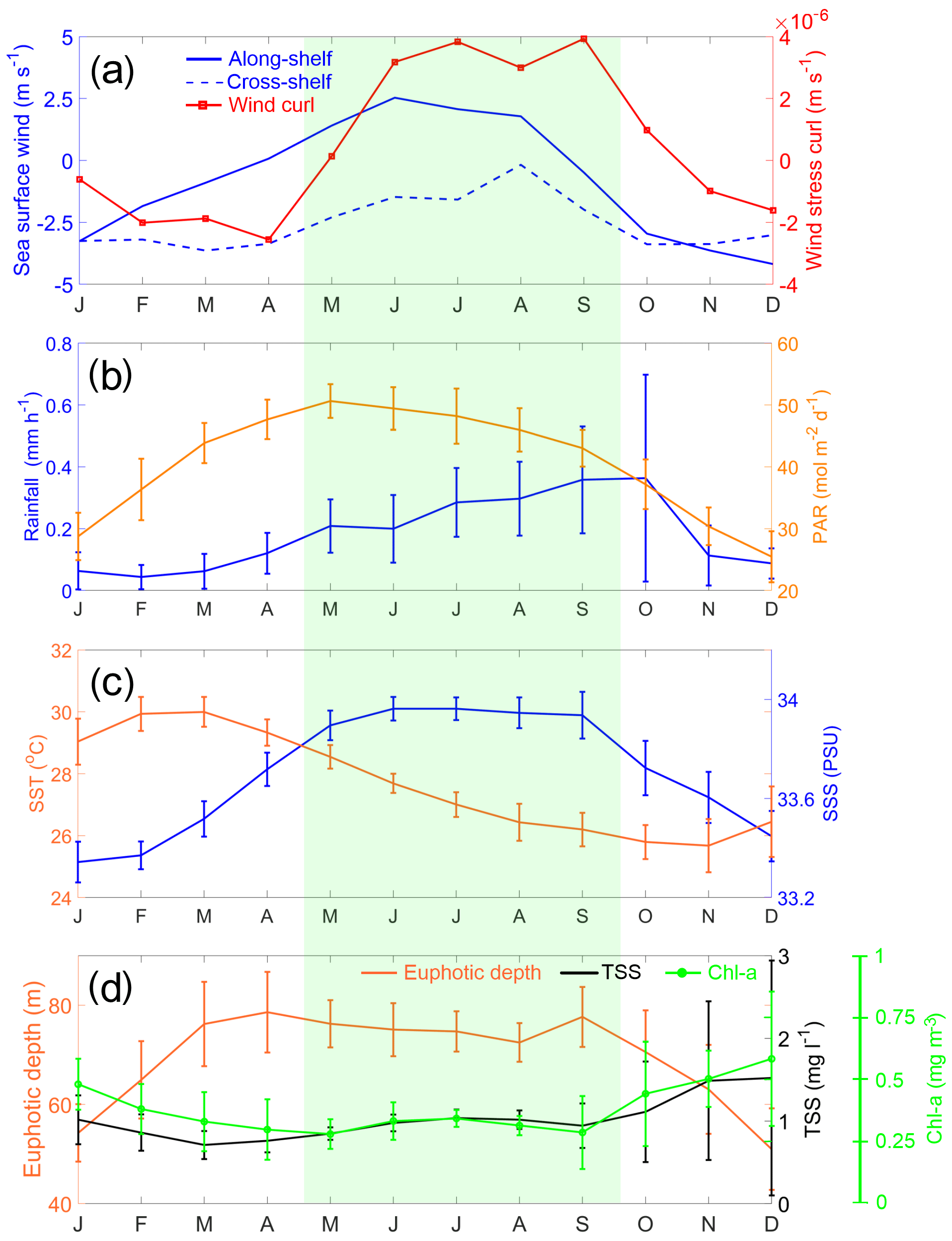
Figure 2 Monthly climatological (a) sea surface wind and wind stress curl, (b) rainfall and PAR, (c) SST and SSS, and (d) euphotic depth, Chl a, and TSS in the study area. The error bar indicates the standard deviation (STD). The shaded area indicates the upwelling season.

3 Results

3.1 Temporal and spatial variations of environmental factors in the HEC

Figure 2 shows the climatological monthly variations of the environmental factors in the study area. As shown in Fig. 2a, the mean along-shelf component of the SSW is positive from May to September, with the strongest value of 2.5 m s⁻¹ occurring in June. In the rest of the months, the along-shelf components of the SSW and wind stress curl are negative. The cross-shelf component of the SSW is also negative. The changes in the wind direction show that the study area is mainly controlled by the Asian monsoon. The period of UEH is coherent with that of the positive along-shelf wind and the wind stress curl from May to September (green shading in Fig. 2a–d), indicating the effects of SSW and wind stress curl on coastal upwelling.

The rainfall in the study area increases monotonically from February to October and peaks in October with a value of 0.37 mm h⁻¹ (Fig. 2b). After October, the rainfall decreases rapidly to 0.10 mm h⁻¹ in November. The rainfall in winter (December, January, and February) was less than 0.10 mm h⁻¹. Differently from the rainfall, the mean photosynthetically active radiation (PAR) in the study area reaches its maximum value of 50 mol m⁻² d⁻¹ in May, indicating its dependence on the annual movement of the sun. The monthly climatological distribution of the SST is similar to that of the PAR, while the highest (lowest) SSS occurred in March (October and November) following the amount of rainfall (Fig. 2c).

For the euphotic depth, the average values in the study area are greater than 50 m all year around and reach 70 m in the months of March to October (Fig. 2d). In contrast, the TSS concentration is less than 1.0 mg L⁻¹ from January to September and reaches the highest value of 1.5 g L⁻¹ in December. Similar to the TSS, the mean Chl a concentration in the study area has smaller values of less than 0.3 mg m⁻³ from March to September, although the UEH occurs in the summer months (green shading in Fig. 2).

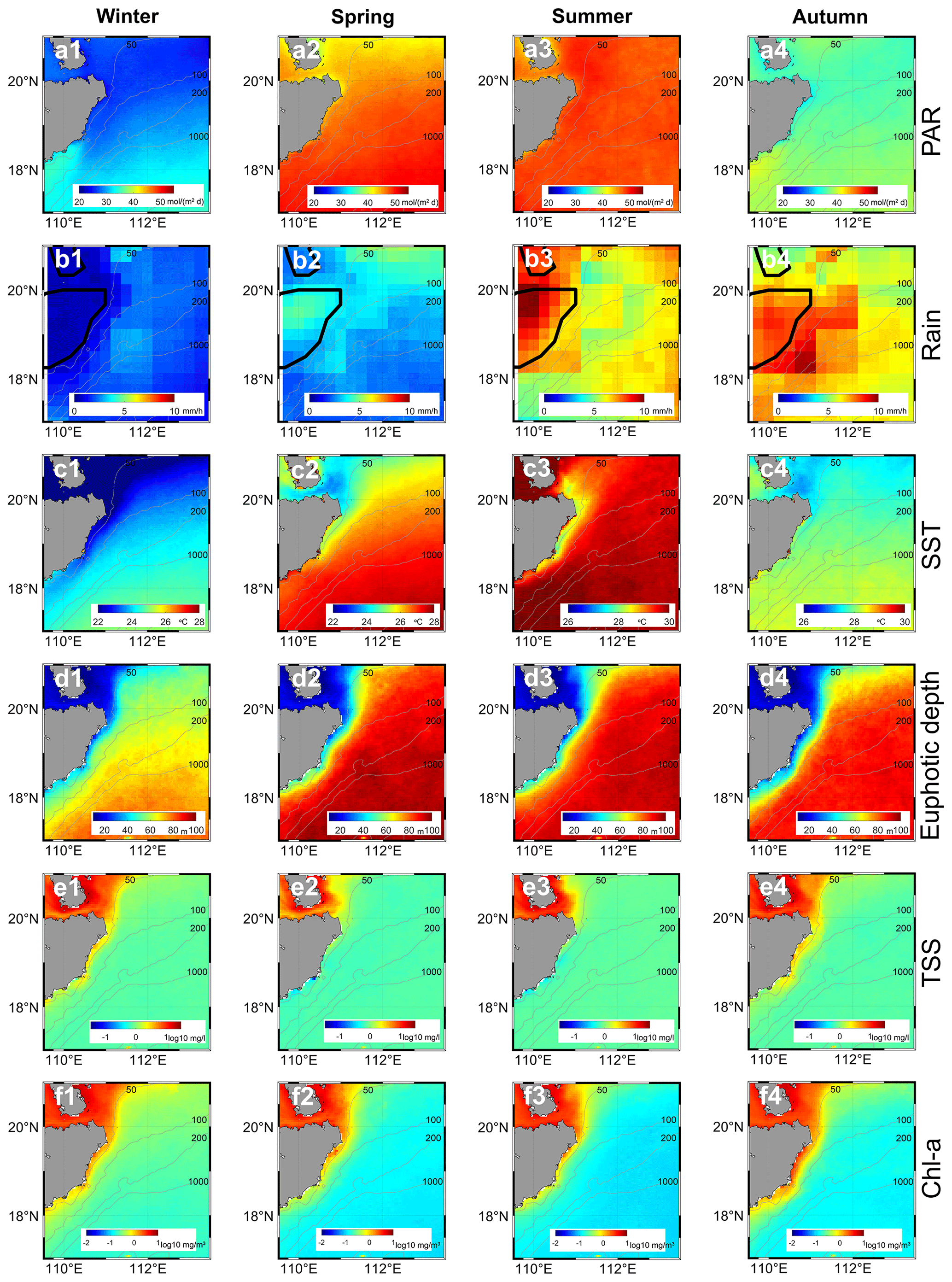
Figure 3 Seasonal climatological (a1–a4) PAR, (b1–b4) rainfall, (c1–c4) SST, (d1–d4) euphotic depth, (e1–e4) TSS, and (f1–f4) Chl a. The columns correspond to winter, spring, summer, and autumn. The unit of the numbers on the isobaths is meters.

Figure 3 shows the spatial distributions of seasonal climatological environmental parameters. The PAR is almost homogeneous in the study area (Fig. 3a). The values are approximately 20–30 mol m⁻² d⁻¹ in winter, reach 50 mol m⁻² d⁻¹ in the spring and summer, and then decrease to approximately 30–40 mol m⁻² d⁻¹ in autumn.

The rainfall rate is less than 5 mm h⁻¹ in winter (Fig. 3b). In spring and summer, the rainfall peaks in Hainan Island, while the high-precipitation area is located on Hainan Island and in the HEC area in autumn. The rainfall rate is as high as 10 mm h⁻¹ in summer and autumn. Furthermore, as the high-precipitation area is located on land, the heavy rain is transformed into runoff, which carries nutrients into the sea. Thus, the temporal and spatial variations in the rainfall rate likely induce variations in the input of terrestrial materials.

The SST exhibits remarkable seasonal variability (Fig. 3c). Generally, the SST is high in spring and summer and low in winter and autumn. Moreover, the SST is lower in coastal waters than in ocean areas in winter and spring, which is modulated by the prevailing southwestward current along the coastline of Guangdong (Ding et al., 2018). In summer, a region identified by low SST (<29 ^∘C) values, i.e., the UEH, is observed to the northeast of Hainan Island.

The spatial distribution of the euphotic depth is consistent with the bathymetric distribution (Fig. 3d). The euphotic depth in spring and summer is approximately 20–30 m within water depths of less than 50 m, whereas it is approximately 100 m in the deeper water. In winter and autumn, the euphotic depth is 20–30 m within water depths of less than 70 m. Moreover, the euphotic depth decreases to 60–80 m in the deeper water. As the latitude of the study area is low, the illumination is not the limiting factor. These variations in the euphotic depth likely affect the vertical distribution of phytoplankton in the water.

Similarly, the TSS concentration is higher in the coastal area and lower in the ocean area (Fig. 3e). Moreover, the TSS concentration is less than 0.3 mg L⁻¹ in spring and summer in the HEC area. However, the TSS concentration increases to 3.0 mg L⁻¹ at water depths of less than 70 m in autumn and winter.

The Chl a concentration is higher in the coastal area than in the open-ocean area (Fig. 3f). In winter and autumn, the Chl a concentration is higher than 1.0 mg m⁻³ in water shallower than 70 m. In spring, the concentration decreases to 0.5 mg m⁻³. However, the Chl a concentration decreases to approximately 0.3 mg m⁻³ in summer. In addition, the high concentration is approximately 1.0 mg m⁻³ in the nearshore area with water depths less than 20 m.

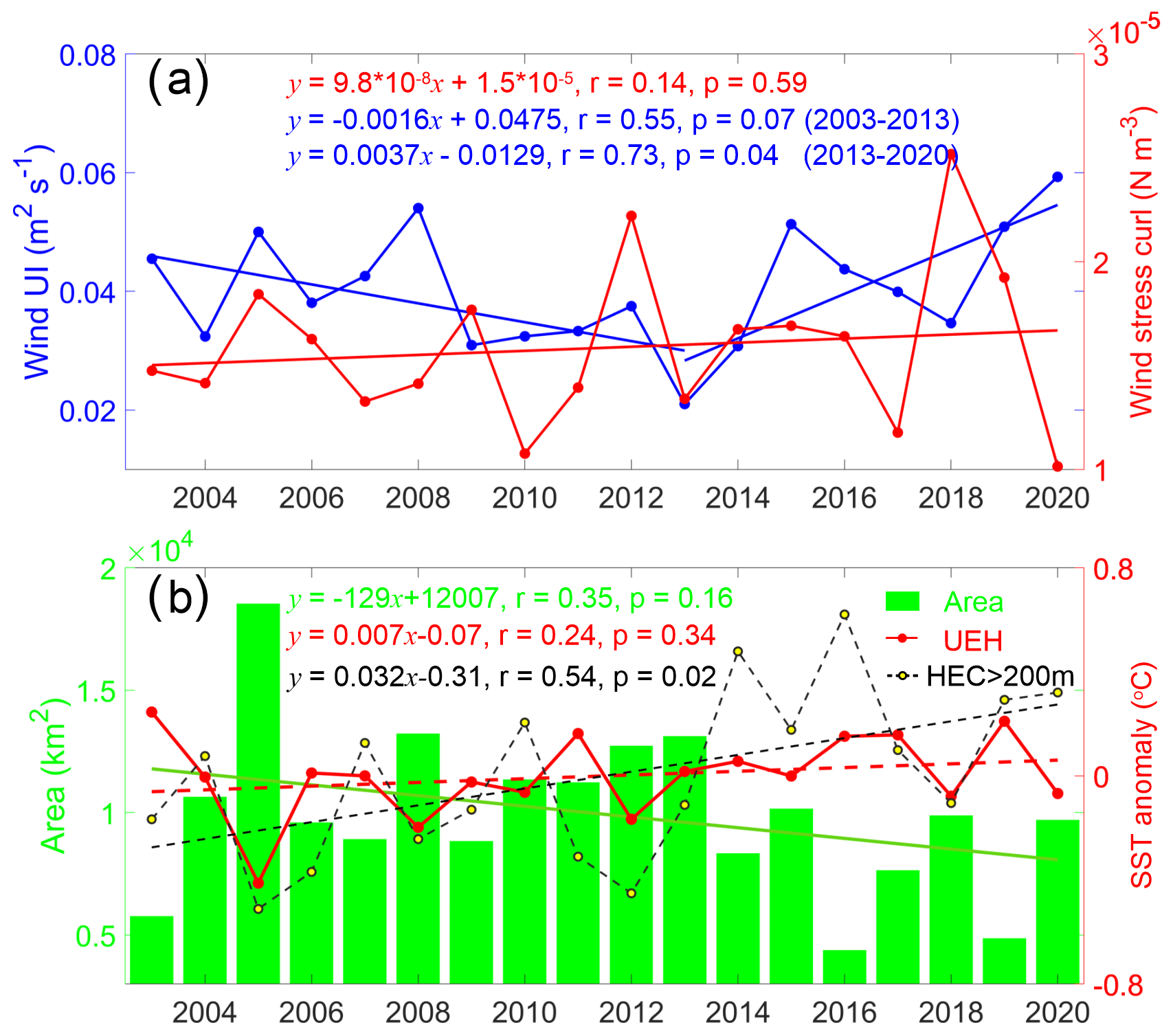
Figure 4 Time series of upwelling index (UI) and upwelling characteristics. (a) Time series of mean sea surface wind UI and wind stress curl in HEC region. The dotted blue curve denotes the mean UI during June–August; the dotted red curve is mean wind stress curl during June–August; and the blue and red curves are the trends of the UI and wind stress curl, respectively. (b) Time series of upwelling area and SST. The green bar denotes the area of UEH region. The dotted red and black curves denote mean SST of the UEH region and the slope region (depth >200 m) in HEC, respectively. The green, red, and black lines are the trends of the upwelling area and the mean SST in UEH and slope area, respectively.

3.2 Variabilities in upwelling

The UI derived from the wind stress and wind stress curl in the HEC are shown in Fig. 4. The results reveal that the wind UI decreased from 2003 to 2013 and increased from 2014 to 2020, probably due to the phase switching of the Pacific Decadal Oscillation (PDO) in 2014 (Qin et al., 2018). Overall, the wind UI associated with alongshore wind stress exhibited an increasing trend from 2003 to 2020. Moreover, the wind stress curl exhibited a weak increasing trend from 2003 to 2020 in the study area.

The time series of the area and SST of UEH are shown in Fig. 4b. The upwelling area exhibited a downward trend from 2003 to 2020. Moreover, the mean SST in UEH exhibited an increasing trend. Though the statistical confidence is less significant due to limited data length (only 18 years), the trends of both the area (−129 km² yr⁻¹) and mean SST (0.007 ^∘C yr⁻¹) indicate that the UEH gradually weakened from 2003 to 2020. However, we checked the mean SST of the background (>200 m in HEC; black curve in Fig. 4b). It shows that the background SST increases much faster than that in UEH. Therefore, we conclude that the upwelling is enhanced by the stronger wind stress and curl in relation to the background of SST becoming stronger.

The time series of UEH area and UI exhibit interannual variations. High UI and wind stress curl values occurred in 2005, 2008, 2012, 2015, and 2018, which coincided with the large areas of upwelling in these years. Low UI values occurred in 2004, 2006, and 2009, which coincided with the small areas of upwelling in these years.

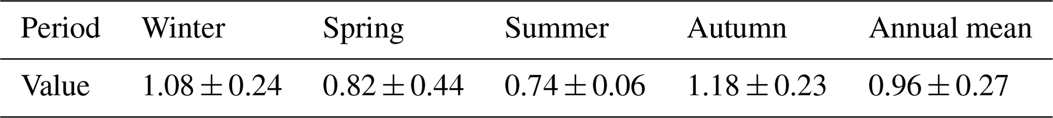
Table 1 Climatologically seasonal mean of the Chl a concentration in the UEH.

3.3 Variabilities in Chl a concentration in the UEH

The time series of the spatial mean of the Chl a concentration in the UEH is shown in Fig. 5. The Chl a concentration is unexpectedly low from April to September, i.e., the upwelling season (as shown in Fig. 5a–b). The climatological mean Chl a concentration is the lowest in summer ( 0.74 mg m⁻³, as shown in Fig. 5b and Table 1), which indicates the relatively limited effect of upwelling on the Chl a concentration in the HEC. On the other hand, the mean Chl a concentration in the UEH is highest in autumn (1.18 mg m⁻³) and almost twice as high as that in summer. In October, the mean Chl a concentration reaches 1.4 mg m⁻³.

The interannual variations of the spatial mean of the Chl a concentration in UEH are also shown in Fig. 5. The Chl a concentration in the UEH was high in 2003, 2006–2007, 2009–2010, 2013, 2016, and 2019. The Chl a concentrations in these years were 2–4 times (ranging from 1.0 to 1.8 mg m⁻³) those in the other years (2005, 2008, 2011–2012, and 2018). In the remaining years, the Chl a concentration is only approximately 0.5 mg m⁻³ in summer, which is much less than the yearly mean value. In 2018, there were minima for both wind UI and Chl a. However, the maximum of wind stress curl existed in 2018, which was the leading factor for the upwelling process (as shown in Fig. 4a).

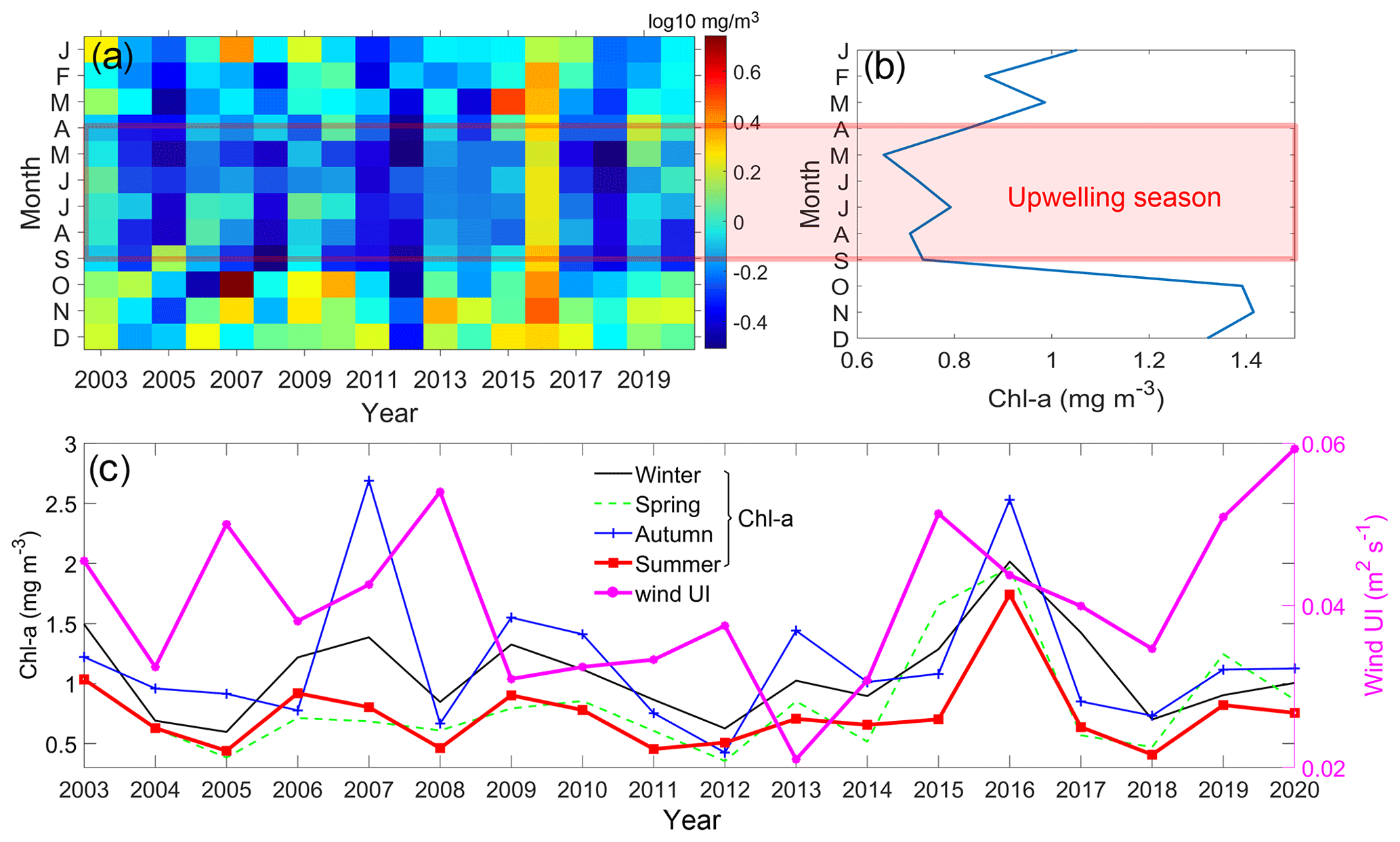
Figure 5 Time series of (a) the spatial mean of the Chl a concentration in the upwelling area, (b) the monthly climatological mean Chl a, and (c) the seasonal mean Chl a and wind UI. The red shading indicates the upwelling season from April to September.

Comparing the time series of Chl a concentration shown in Fig. 5 to the time series of upwelling characteristics, one can see that low UI values coincide with high Chl a concentration in the UEH in most years and vice versa. The correlation coefficient between wind UI and Chl a concentration during 2003–2012 is −0.3, which shows a negative relationship. The main reason for the negative relationship is the low background SST during 2003–2012. It is known that high UI values indicate strong upwelling in the HEC. This means that upwelling is not favorable for Chl a bloom in the UEH. Moreover, one can see that the Chl a concentration is unexpectedly low in the upwelling season, as shown in Fig. 5. Therefore, the results provide new insight into the relationship between marine productivity and upwelling in the UEH. However, the effect of environmental factors and spatial variations on the Chl a concentration needs further investigation.

As the PDO phase changed after 2014, the wind UI and Chl a concentration seem to be positively correlated with each other. There was a strong ENSO event in 2015–2016 and a strong wind stress curl in 2018. A high wind UI and wind stress curl occurred in 2015–2016 combined with a high Chl a concentration. In 2018, though there was a weak wind UI, the strong wind stress curl still induced a strong upwelling process, as shown in Fig. 4. However, a low Chl a concentration occurred in UHE in 2018 (Fig. 5c). This further confirms the limited effects of upwelling on Chl a in the study area. The environmental factors need to be further investigated.

3.4 EOF analysis of Chl a concentration

To further reveal the variations in the Chl a concentration in the HEC, the EOF analysis results are shown in Figs. 6–7. The first four EOF modes of the Chl a concentration explain 60 % of the total variance (Fig. 6). Mode 1 includes an enhanced signal in the coastal waters (<60 m) to the east of Hainan Island. The magnitude of the variability is generally the same throughout the other areas. The corresponding temporal evolution (Fig. 7a) is characterized by strong seasonal cycles, with peaks in October and troughs in May. The climatological mean of the corresponding temporal evolution is negative from April to September and positive from October to March. The negative phase with a large amplitude lasts for 6 months. Therefore, the Chl a concentration is persistently low from April to September. Mode 1 is characterized by the GDCC (Ding et al., 2018). Mode 2 separates the east and northeast coastal waters of Hainan Island. The troughs of the temporal evolution of Mode 2 occur in September and October. The climatological mean peaks in January and December. The strong signals occur in September and October to the east of Hainan Island, which indicates that the Chl a concentration is controlled by rainfall (as shown in Fig. 3b). The other strong signals occur in January and December. Moreover, they are located on the north shelf of the SCS, adjacent to the Qiongzhou Strait to the west. Thus, the result suggests that Chl a concentration is affected by the GDCC.

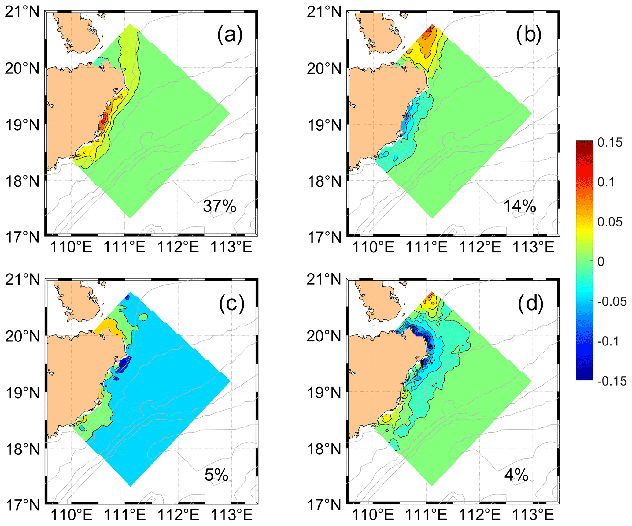
Figure 6 Spatial distributions of the first four EOFs for the Chl a concentration. The variance explained by each mode is labeled.

Mode 3 describes 5 % of the total variance in the Chl a concentration in the coastal regions of Hainan Island. Mode 3 also separates the east and northeast coastal waters of Hainan Island (Fig. 6c). However, the climatological mean of the temporal evolution is positive between June and August. Therefore, the positive phase occurs in summer, revealing an upwelling area to the east and north of Hainan Island. Mode 4 contributes only 4 % of the total variance. The climatological mean of the temporal evolution exhibits strong peaks in July and weak peaks in April, i.e., semiannual variability. High Chl a concentrations occur in the northeast coastal waters of Hainan Island during the upwelling season.

Modes 3 and 4 both describe the upwelling phenomenon along the northeast coast of Hainan Island during summer. The spread of upwelling can be seen clearly in the EOFs of the Chl a concentration in the areas with water depths of less than 100 m along the coastline. However, upwelling described less than 10 % of the total variance in the Chl a concentration, indicating that the contribution of upwelling to productivity in the HEC is limited.

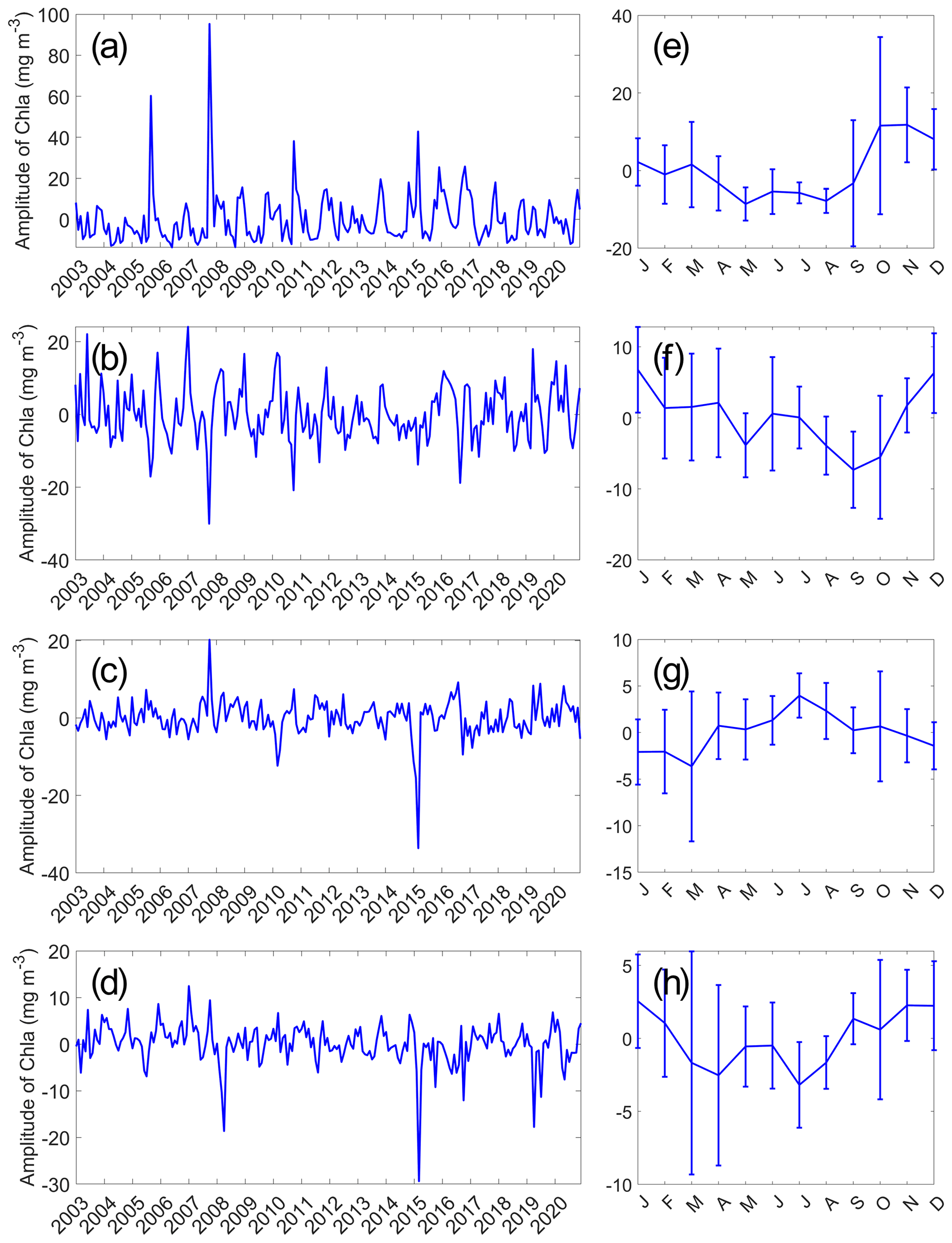
Figure 7 (a–d) Time series and (e–h) climatological mean of the first four EOFs for the Chl a concentration.

3.5 Vertical distribution of the Chl a concentration based on observation data

To examine the vertical distribution of the Chl a concentration in the HEC, two cruise measurement sections are used in this study. Figure 8 shows the oceanographic cruise data collected on 14–15 July 2021 and 2–3 October 2019, illustrating the distribution of the Chl a concentration in summer and autumn, respectively. The pronounced upwelling can be seen on the cross-shelf section observed in July 2021. Both the isotherm and isohaline on the shelf are uplifted toward the shore by upwelling-induced movement. A temperature front can be seen near the sea surface, which is located approximately 50 km away from the coastline (depths of ∼90 m). The thermal fronts are reported by Jing et al. (2016). The fronts induced by upwelling tend to be approximately aligned with the 20–100 m isobath. The high Chl a concentration layer is also uplifted from 80 to 40 m by upwelling, and the Chl a concentration is as high as 1.2 mg m⁻³.

From 2–3 October 2019, the sea surface temperature front disappeared. Jing et al. (2016) found that the front was the weakest in autumn. However, a salinity front occurs approximately 60 km from the coastline in the sea surface. This salinity front indicates that fresh water is injected into the sea surface. Figures 2b, 3b, and 4 show that the rainfall is strong during autumn. The rainfall is input into the sea surface via rainfall and runoff. Thus, the salinity front is generated. In contrast to the upwelling in summer, downwelling occurs in the bottom water and is associated with downwelling-favorable wind forcing. Moreover, abundant Chl a is detected at a depth of 30 m on the shelf, which is shallower than the detection depth in summer, since the euphotic depth is shallower in autumn, as shown in Fig. 3d.

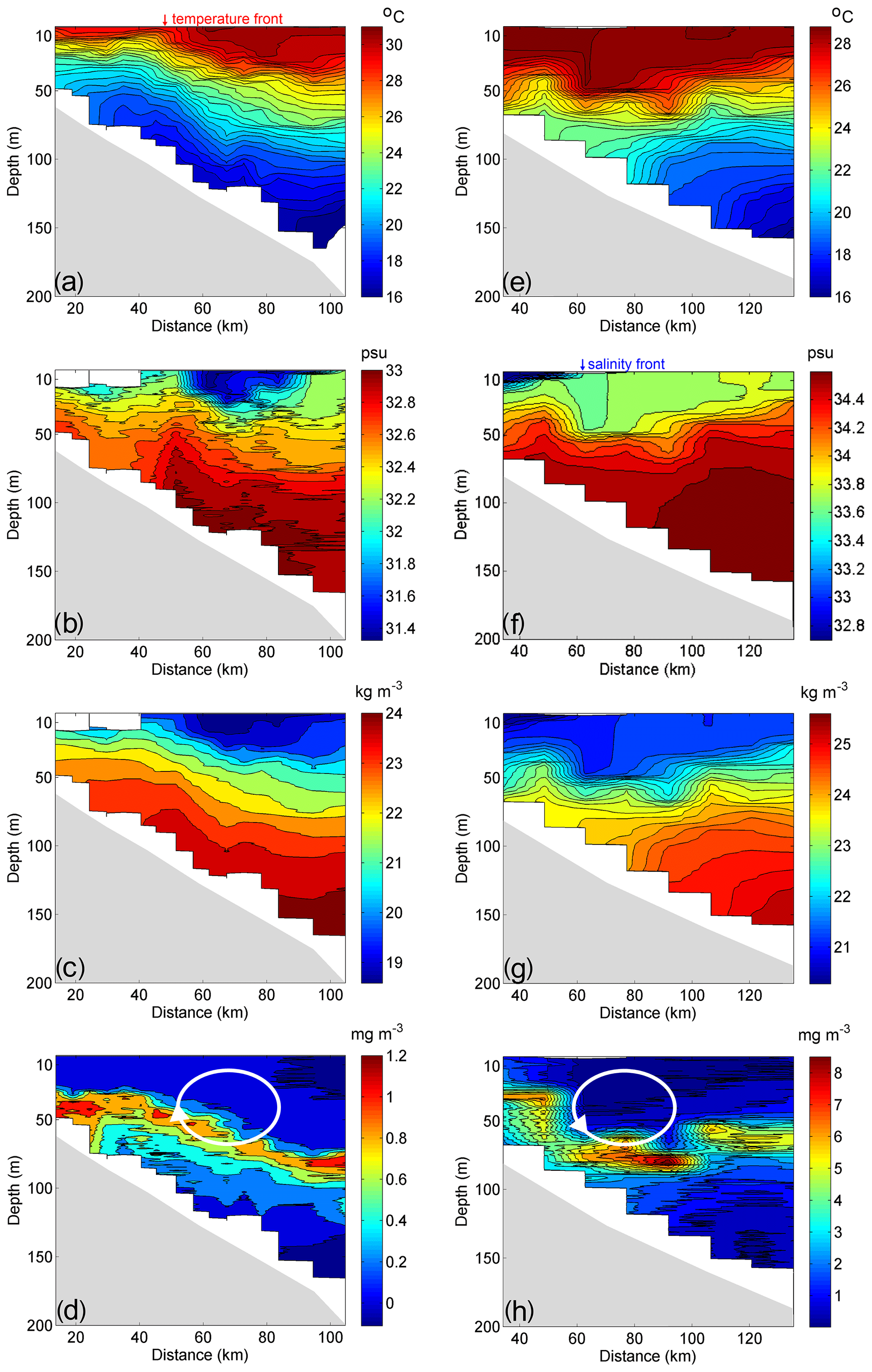
Figure 8 Oceanographic cruise data collected on (a–d) 14–15 July 2021 and (e–h) 2–3 October 2019: (a) and (e) temperature distributions; (b) and (f) salinity distributions; (c) and (g) potential density distributions; and (d) and (h) Chl a distributions. The arrows indicate the location of the temperature and salinity front near the sea surface. The white circle is a diagrammatic sketch for upwelling and downwelling circulation.

4 Discussion

4.1 Relationship with typhoon events

In the NWSCS, the Chl a concentration can be affected by different factors, e.g., typhoons. Typhoon-induced upwelling occasionally occurs in the SCS (Ma et al., 2021; Wang et al., 2020). In the shelf areas, typhoon-enhanced vertical mixing and upwelling play dominant roles in the spatiotemporal behavior of the Chl a concentration (Li et al., 2021a, b). The upwelling transports nutrients into the euphotic zone, which supports Chl a blooms (Ye et al., 2013; Zheng et al., 2021). An increase in the Chl a concentration in the nearshore region off Hainan Island followed typhoon rainfall, with mixing and upwelling effects (Zheng and Tang, 2007). The large-scale peripheral wind vector resulted in the accumulation and enhancement of the Chl a concentration in the nearshore area (Liu et al., 2020). An offshore bloom produced a Chl a peak (4 mg m⁻³) after the typhoon's passage (Zheng and Tang, 2007). These observations illustrate the effects of typhoons on the marine ecosystem in the HEC.

Figure 9 (a) Time series of the number of typhoons that passed by the study area during 2003–2020. (b) Seasonal distribution of typhoons. (c) Trajectories of typhoons during 2003–2020. The orange, red, and blue bars in (a–b) represent the numbers of tropical depressions and tropical storms, severe tropical storms and typhoons, and severe typhoons and super typhoons, respectively. The magenta and black curves in (c) represent the typhoons that passed by the study area in July and October, respectively. The green curves represent the typhoons that passed by the study area in the other months.

Figure 9 shows the time series of the number of typhoons that passed over the HEC during 2003–2020. Sixty-eight typhoons passed across the continental shelf of the NWSCS during this 18-year period. There were interannual variations in the time series of the number of typhoons. As many as nine typhoons were generated and affected UEH in 2013, while fewer than two typhoons passed by the study area in 2004, 2007, 2010, and 2014–2015. Seasonally, 33 typhoons passed by in summer and autumn. As shown in Fig. 5b, a small peak in the mean Chl a concentration occurred in July. Moreover, the Chl a concentration was high in 2013, especially in autumn; furthermore, it varied within the range of 0.7–1.5 mg m⁻³ and coincided with the occurrences of nine typhoons. This indicates that the high Chl a concentrations were related to the typhoons. However, typhoons occur on the synoptic scale and influence the coastal area for several days. Therefore, these processes seem to have a limited effect on the monthly mean Chl a concentration.

4.2 Role of the coastal current

The current in the NWSCS contributes significantly to the transport of low-salinity water, nutrients, and phytoplankton, and it also affects the ecological environment (Ding et al., 2018; Meng et al., 2017). The shelf circulation pattern is dominated by monsoons, tides, buoyancy forcing, and topography. Due to the changes in the wind direction, the current direction changes in the different seasons. In autumn and winter, the current in the NWSCS is predominantly southwestward. It changes to be northeastward in summer (Ding et al., 2018). The monsoon plays an important role in the current, which induces onshore and offshore Ekman transport on the shelf during the winter and summer monsoons, respectively. Gan et al. (2013) found that transport was induced by amplified geostrophic transport during downwelling events. Here, we used geostrophic current retrieval from along-track satellite altimeter data on the shelf of the NWSCS to reflect the role of the coastal current in relation to the Chl a concentration.

The latitudinal distribution of the climatological along-track SLA is shown in Fig. 10. The climatological sea surface in the shelf side is higher than that in the ocean side in October, November, and December. Additionally, the sea surface on the shelf was lower than that in the ocean from April to August. The geostrophic current shows that the current was positive (northeastward) between April and August, and it was negative (southwestward) between October and March. The climatological geostrophic current in September was approximately 0 m s⁻¹, which indicates that the current direction changed frequently. The climatological geostrophic current was stronger than 0.1 m s⁻¹ in summer, and it was strongest in October at approximately 0.17 m s⁻¹.

In autumn and winter, the abundant nutrients in the GDCC, which were provided by the Pearl River, likely supported the high food availability to the phytoplankton (Yang and Ye, 2022). The GDCC was characterized by a high TSS (Figs. 2d and 3e). TSS is synergistic with the concentration of dissolved nitrogen and is the dominant factor affecting the Chl a concentration (López Abbate et al., 2017). The distribution of the monthly climatological Chl a concentration (Fig. 5b) was similar to that of the geostrophic current. In summer, the Chl a concentration was low during the northeast oligotrophic current. In winter, the Chl a concentration was high during the southwest nutrient-rich current. Figure 10c presents the time series of the geostrophic current and Chl a concentration. The negative current and high Chl a concentrations mainly occurred in autumn and winter, which demonstrates the crucial role of the current in Chl a variations.

4.3 Role of rainfall

The phytoplankton responded more positively to the increased precipitation in the coastal waters (Thompson et al., 2015). Kim et al. (2014) reported that the increase in wind speed accompanied by rainfall was a major contributor to the Chl a concentration. The precipitation directly deposits the nutrients in the air into the seawater. In addition, most of the rainfall on land runs over the land surface into the rivers and eventually into the ocean, transporting nutrients to the ocean. Therefore, rain plays an important role in the variability of phytoplankton in coastal waters.

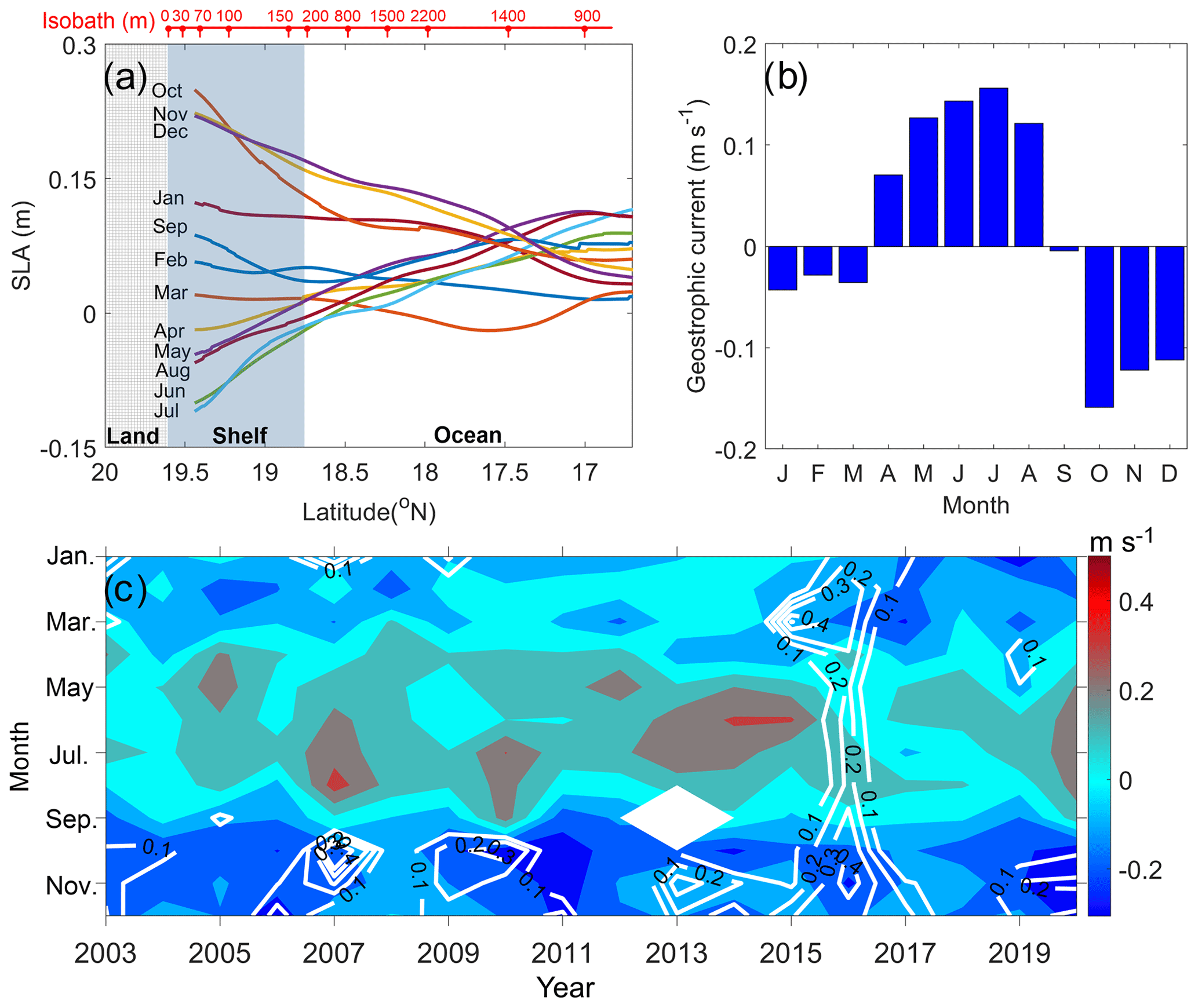
Figure 10 (a) Latitudinal distribution of climatological along-track SLA (track number: 114). (b) Geostrophic current retrieval from climatological along-track SLA. (c) Time series of geostrophic current (contours) and Chl a concentration (white contour curves). The shadings in (a) represent the ocean, continental shelf, and land areas, respectively. The red bar with numbers in (a) indicates the water depth of the along-track SLA data. The values in (c) are the exponents of the Chl a concentration.

Figure 11 shows the time series of the monthly mean rainfall rate and Chl a concentration. The rainfall rate was high in the summer and autumn, ranging from 0.3 to 1.4 mm h⁻¹. In October in 2007–2017, the monthly mean rainfall rate (>0.5 mm h⁻¹) coincided with the high Chl a concentration.

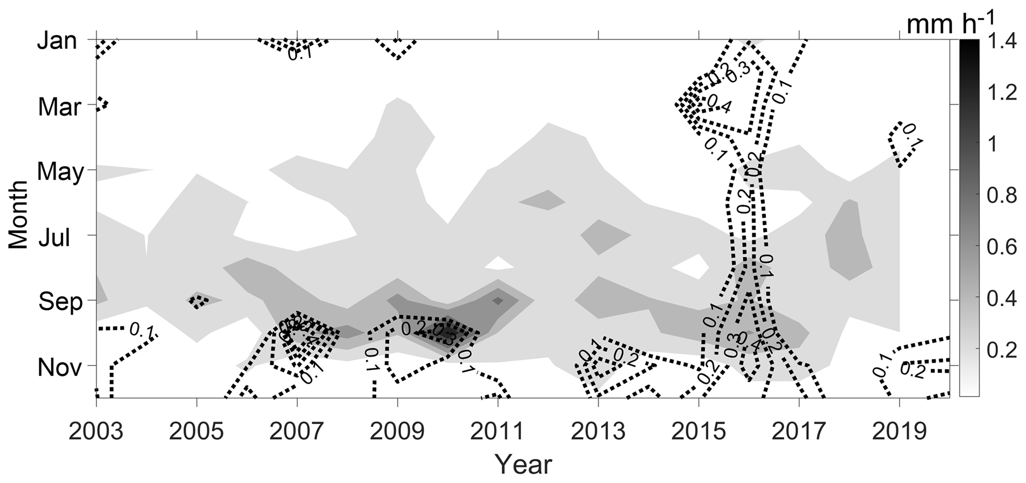
Figure 11 Time series of the rainfall rate (contours) and Chl a concentration (dotted curves with text labels). The values on the contours are the exponents of the Chl a concentration.

Runoff is the main source of silicate in coastal waters (Zhang et al., 2003). Chen et al. (2016) observed that the concentration of silicate was as high as 2–12 µmol L⁻¹ in the coastal waters of the HEC and had a positive correlation with the Chl a concentration. Wang et al. (2018) found that diatoms contributed 88.11 % and 85.81 % of the total phytoplankton abundance in the northern SCS in May and October, respectively. The Chl a concentration can increase by 0.3 mg m⁻³ after a rainfall event (Zeng et al., 2022). Moreover, in Mode 2 of the EOFs (Figs. 6–7), the positive phase of the Chl a concentration occurred off the east coast of Hainan Island in October, which is near the estuary of the Wanquan River. Therefore, the runoff caused by the high rainfall rate triggered the high Chl a concentrations in the HEC.

4.4 Relationship with ENSO events

ENSO has an indirect positive effect on the Chl a concentration through its influences on precipitation, winds, SST, and turbidity (López Abbate et al., 2017). During El Niño events, the southwesterly wind anomalies would enhance the coastal upwelling in the SCS (Jing et al., 2011; Kuo et al., 2008). The positive southwesterly wind anomalies lag the El Niño event by several months (Hong and Zhang, 2021; Huynh et al., 2020). The reverse occurs during La Niña events.

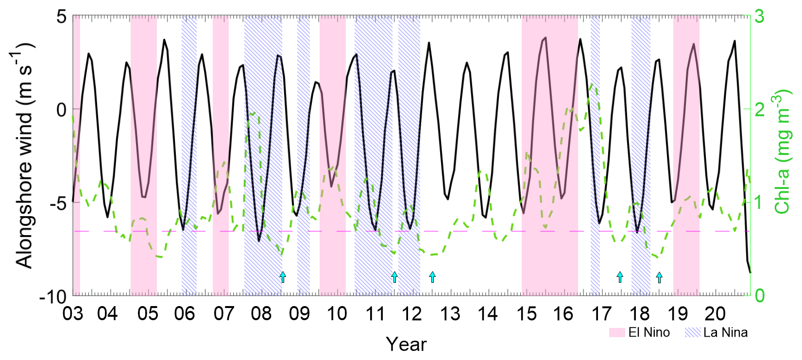
Figure 12 Time series of Chl a (green curve) and along-shelf wind (black curve). Stripes point out the El Niño (magenta) and La Niña (blue) events. The blue with black arrows point out the minima value of Chl a concentration. The dashed magenta lines indicate high Chl a concentrations during El Niño events.

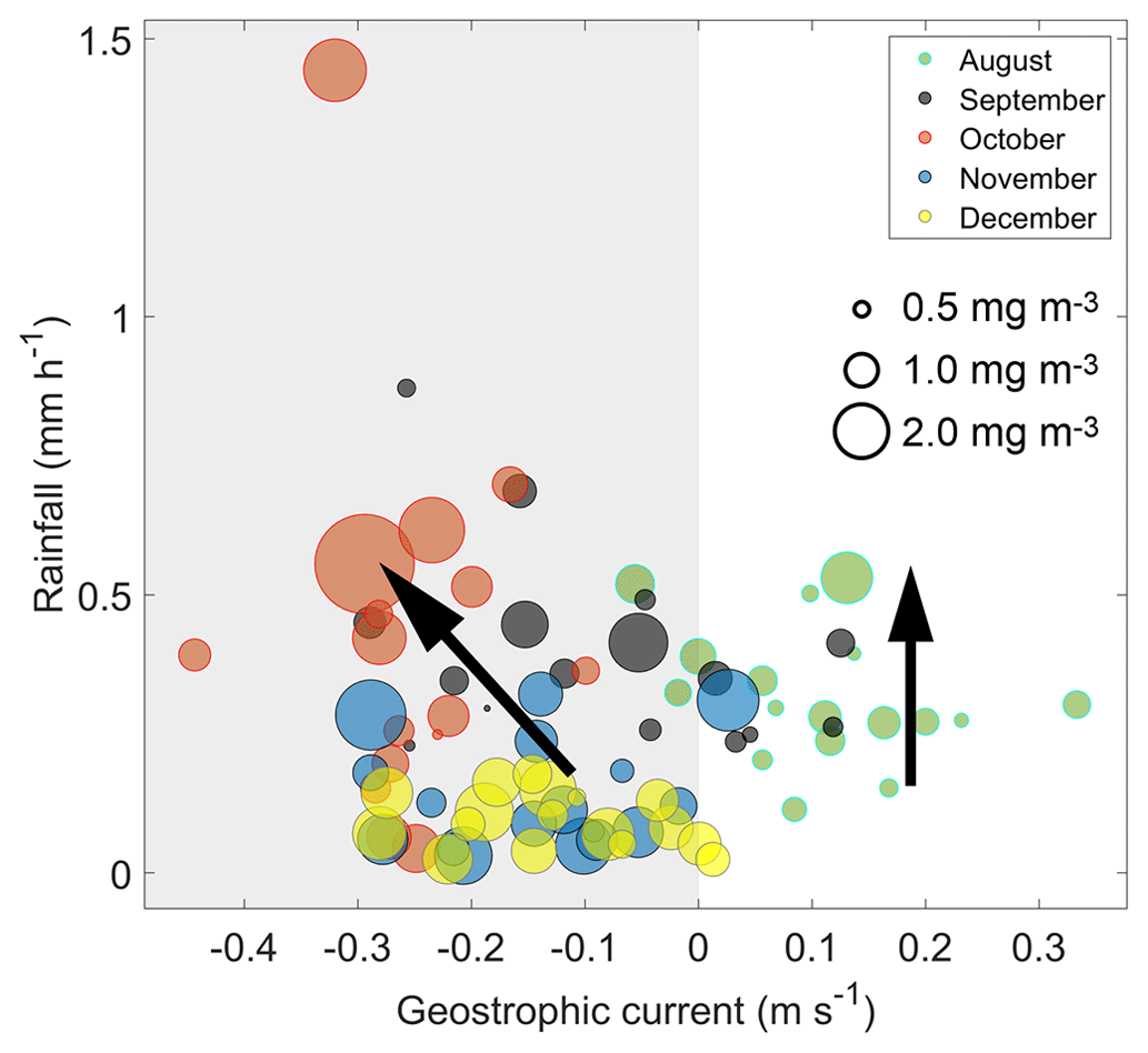
Figure 13 Bubble diagram showing the relationships between the geostrophic current and rainfall and the Chl a concentration. The size of the bubble represents the Chl a concentration. The left panel in gray represents the southwestern along-shelf current in winter. The right panel represents the northeastern along-shelf current in summer. Black arrows represent the relationship between the geostrophic current and rainfall and the Chl a concentration.

In the upwelling season, i.e., summer, the wind was larger during El Niño events than during La Niña events (Fig. 12). In summer 2005, after an El Niño event, the wind stress and upwelling area were much larger than that in summer 2004 before the event. The upwelling area increased in 2005 as shown in Fig. 4b, while the Chl a concentration decreased to 0.6 mg m⁻³ in June 2005. During 2015–2016, the summer wind stress and curl were both strong, and the upwelling area was larger than that in 2014. There was an anomalously high Chl a concentration that occurred in June 2016. Jing et al. (2011) reported an analogously high Chl a concentration anomaly in 1998. We should notice that a maximum SST occurred in summer 2016, with a maximum in terms of Chl a concentration, while minimum values of background SST (Fig. 4b) occurred in summer of the years 2008, 2011, 2012, 2017, and 2018 combined with a minimum in terms of Chl a concentration (arrows in Fig. 12). Therefore, ENSO events regulated the Chl a concentration of the upwelling through wind stress and background SST. Further research is required to investigate the relationship between the Chl a variability and ENSO in the HEC.

In autumn, especially October, the spatial mean Chl a concentration in the upwelling area was as high as 1.18 ± 0.23 mg m⁻³. The precipitation was heavier during La Niña events (i.e., in 2005, 2007, 2010–2011, and 2016) than during El Niño events. Furthermore, the along-shelf current from the north was crucially important to the Chl a concentration. There was a positive relationship between the Chl a anomalies and the La Niña events.

4.5 Mechanisms of Chl a variations in the HEC area

Figure 13 shows the relationships between the geostrophic current and rainfall and the Chl a concentration during 2003–2020. The Chl a concentration increased with increasing rainfall in August, i.e., the upwelling season. The rainfall was converted to runoff and flowed into the coastal waters. The Chl a concentration in summer was mainly regulated by upwelling processes (Jing et al., 2011). Therefore, the increased precipitation and weaker upwelling processes could have induced the increased Chl a concentration in the HEC (upward arrow in Fig. 13).

In autumn and winter, the Chl a concentration was increased by the increases in both rainfall and the northeastward coastal current (oblique upward arrow in Fig. 13). In October, the heaviest rainfall and the strongest current coincided with the highest Chl a concentration. The coastward wind component was strongest in October (Fig. 2a), as was the northeast monsoon, which induced coastward Ekman transport (Xuan et al., 2021). The downwelling movement transported the nutrients from the rivers and the coastal current to the middle and under layers on the shelf, which promoted an increase in silicate-favoring phytoplankton. The cruise data provide evidence of the high Chl a concentrations over the shelf (Fig. 8h).

5 Conclusions

In this study, in situ observations and monthly satellite observations from 2003 to 2020 are used to investigate the spatiotemporal variability in the Chl a concentration in the HEC area. Along-track satellite altimeter data for the continental shelf of the NWSCS were used to retrieve the geostrophic current. In addition, cruise data obtained in October 2019 and July 2021 were used to examine the vertical structure of the Chl a concentration during the three observational seasons.

Due to global warming, the SST of the core upwelling area (within a depth of 100 m) in summer increased while the area decreased, which indicates that the UEH weakened during the 18-year study period. The EOF analysis of the Chl a concentration revealed that it exhibited strong seasonal and interannual variability in the NWSCS. The climatological average Chl a concentration mostly peaked near the coast in autumn at 1.18 mg m⁻³. However, the Chl a concentration in the core upwelling area was lowest during the upwelling season at approximately 0.74 mg m⁻³ in summer, which contradicts the previous conclusion of a high-productivity upwelling system.

ENSO events regulated the Chl a concentration of the upwelling area through wind stress and background SST. The interannual variations in the spatial mean of the Chl a concentration were consistent with the ENSO events. In El Niño years, the Chl a concentration decreased to a lower level in summer. However, the summer Chl a concentration increases to as high as 1.0 mg m⁻³ with weak upwelling. The complicated relationship between the Chl a variability and ENSO in the HEC needs further pursuing.

Both the along-shelf current from the north and the precipitation were crucial factors controlling the Chl a concentration in the UEH area. The downwelling movement transported nutrients from the rivers and the coastal current to the middle and lower layers on the shelf, which promoted an increase in silicate-favoring phytoplankton. These results provide scientific evidence for the development of the marine economy in the upwelling area.