Fortnightly variability of Chl a in the Indonesian seas

Twenty years of daily MODIS-Aqua ocean color observations (2002–2022) are used to identify periodic variability of near-surface chlorophyll (Chl a) in the Indonesian seas. The frequency spectrum of Chl a is dominated by the mean and low-frequency monsoonal variability; however, a prominent peak around the fortnightly tidal period, MS_f, is present. Harmonic analysis is used to quantify and map the fortnightly Chl a signal, which is discovered to be significant along the continental shelves of NW Australia and at several sites associated with narrow passages between the Lesser Sunda Islands, within the Sulu Archipelago, and at a few other sites in the Philippines Archipelago. Fortnightly variability at the shallow coastal sites is attributed to the spring–neap cycle of barotropic ocean currents, while we hypothesize that the variability in deeper water near the island passages is due to the modulation of vertical nutrient fluxes by baroclinic tidal mixing. The results document the significance of tidal mixing and highlight the heterogeneous character of biophysical processes within the Indonesian seas.

1 Introduction

The Indonesian Archipelago is a unique region of the world characterized by the warmest sea surface temperatures (SSTs) of the ocean, and it is a key region of the climate system (Nagai and Hibiya, 2015). The Indonesian seas play a critical role in the climate system, with the Indonesian Throughflow (ITF) being the only tropical pathway connecting the global oceans (Sprintall et al., 2014). Pacific warm pool waters passing through the Indonesian seas are cooled and freshened by strong air–sea fluxes and vertical mixing induced by internal tides to form a unique homohaline water mass (Indonesian Throughflow Water or ITW) that can be tracked across the Indian Ocean basin and beyond (Atmadipoera et al., 2022). The Indonesian seas lie at the climatological center of the atmospheric deep convection associated with the ascending branch of the Walker Circulation (Clement et al., 2005). Regional SST variations cause changes in the surface winds that can shift the center of atmospheric deep convection, subsequently altering the precipitation and ocean circulation patterns within the entire Indo-Pacific region (Ropelewski and Halpert, 1987). The tidal vertical mixing induces an averaged cooling of 0.5 ^∘C of the Indonesian warm SST (Koch-Larrouy et al., 2008), which in turn reduces the precipitation by 20 % (Koch-Larrouy et al., 2010) and regulates the amplitude and variability of El Niño–Southern Oscillation (ENSO), the Indian Ocean Dipole (IOD), and the Madden–Julian Oscillation (MJO) (Sprintall et al., 2019). Indeed, models that include tidal mixing have improved representation of ENSO, IOD, and MJO patterns (Susanto et al., 2005; Sprintall et al., 2019).

Previous studies have shown that SST patterns in the Indonesian seas are highly influenced by tidal mixing as well as monsoonal winds, surface heat fluxes, and the ITF (Koch-Larrouy et al., 2010; Kida and Wijffels, 2012; Sprintall et al., 2014, 2019). The spring–neap cycle of the tides has been measured in the SST using satellite data (Ray and Susanto, 2016) and simulated using models (Nugroho et al., 2018). In fact, only model simulations that include tides (Koch-Larrouy et al., 2007; Nugroho, 2017; Nagai et al., 2017, among others) are capable of reproducing the homohaline water (ITW).

However, the complexity of the atmospheric and ecosystem's response to tidal mixing remains poorly understood and is a topic of ongoing research. It is a challenge to disentangle the variability connected with long-term trends and monsoonal and seasonal processes, which are each heterogeneous across the domain (Susanto and Ray, 2022). Recent joint analysis of chlorophyll a (Chl a), winds, ocean currents, and active tracers (Mandal et al., 2022); Chl a, winds, sea surface temperature, and sea level (Wirasatriya et al., 2021); Chl a, climate indices, precipitation, and river runoff (Siswanto et al., 2020); and sea level, winds, and stratification (Devlin et al., 2018) are all examples of multi-variable approaches to understanding the low-frequency dynamics of this complex region.

The goal of this study is to document the variability of upper-ocean Chl a concentration associated with the spring–neap tides throughout the Indonesian seas and nearby waters (from 23^∘ S to 28^∘ N and 87 to 148^∘ E). Spring–neap variability arises when the vector sum of currents at the M₂ and S₂ tidal frequencies are rectified or otherwise interact to produce modulations of bottom stress or internal wave-driven mixing with a period of 14.77 d (denoted with the Darwin symbol, MS_f), phase-locked with the astronomical forcing. At least three different mechanisms could explain the association of increased Chl a with spring–neap currents (Xing et al., 2021): a modulation of the tidally driven turbulent flux of nutrients into the euphotic zone, a modulation of suspended sediment concentration affecting the intensity of photosynthetically active radiation (which ought to decrease apparent Chl a), and a modulation of resuspended Chl a associated with the microphytobenthos. The present study uses daily averages of Chl a inferred from multi-spectral imagery acquired by the MODIS-Aqua mission from 2002 to 2022. It is motivated by several ongoing studies which seek to model the physical and biological dynamics of the ITF (Gutknecht et al., 2016; Nugroho et al., 2018). The results focus on observations of Chl a variability rather than its causes; however, satellite altimetry provides independent evidence for nonlinear interaction of M₂ and S₂ currents and suggests several sites where field investigations could identify the drivers and assess the dynamics of Chl a variability in detail.

Previous studies of Chl a variability employing satellite ocean color measurements have mentioned the challenges associated with data gaps due to cloudiness, sunglint, and water-type variability (Palacios, 2004; Susanto et al., 2006; Garcia and Garcia, 2008). A variety of approaches to overcoming these difficulties has been used to either fill data gaps (Yang et al., 2021) or phase-average the data according to days after full moon, for example, in the analysis of suspended sediment (Shi et al., 2011). Recently, another approach based on the wavelet analysis of 4.5 years of Himawari-8 imagery was used to study Chl a, which was capable of identifying seasonal and spring–neap variability (Xing et al., 2021). Given the long, 20-year, duration of the MODIS records considered here, we have found that least-squares harmonic analysis is adequate to quantify variability, even with the data gaps and noise, as detailed below. A similar approach highlighted spring–neap variability from 12 years of high-resolution SST data in the same region (Ray and Susanto, 2016).

2 Data and methods

The Chl a dataset used here consists of the Level-3 “GlobColour daily MODIS product”, version 2018.4, which is an estimate of the near-surface Chl a concentration in units of milligrams per cubic meter obtained from MODIS-Aqua data using a semi-analytical model (the Garver–Siegel–Maritorena (GSM) product; Maritorena and Siegel, 2005; Maritorena et al., 2010). The GSM product is based on representing the spectrum of outgoing radiation with contributions due to Chl a, dissolved organic matter, and suspended particular matter and estimating these quantities from a weighted average of spectral data. The product provides daily estimates, although the constituent measurements may occasionally fall outside of the calendar date of the product. For the purpose of harmonic analysis, the measurements are treated as if they occur at 12:00 GMT of the product date. The spatial resolution of the gridded GSM data is approximately 5 km.

A map of the number of Chl a observations per pixel illustrates the influence of clouds and other processes responsible for data gaps (Fig. 1). The region just off the northwest coast of Australia contains the most data, the longest time series comprising about 10 years of observations, although this is only about half the total possible if every daily data value were populated. Individual pixel time series typically contain between 500 and 1000 data values.

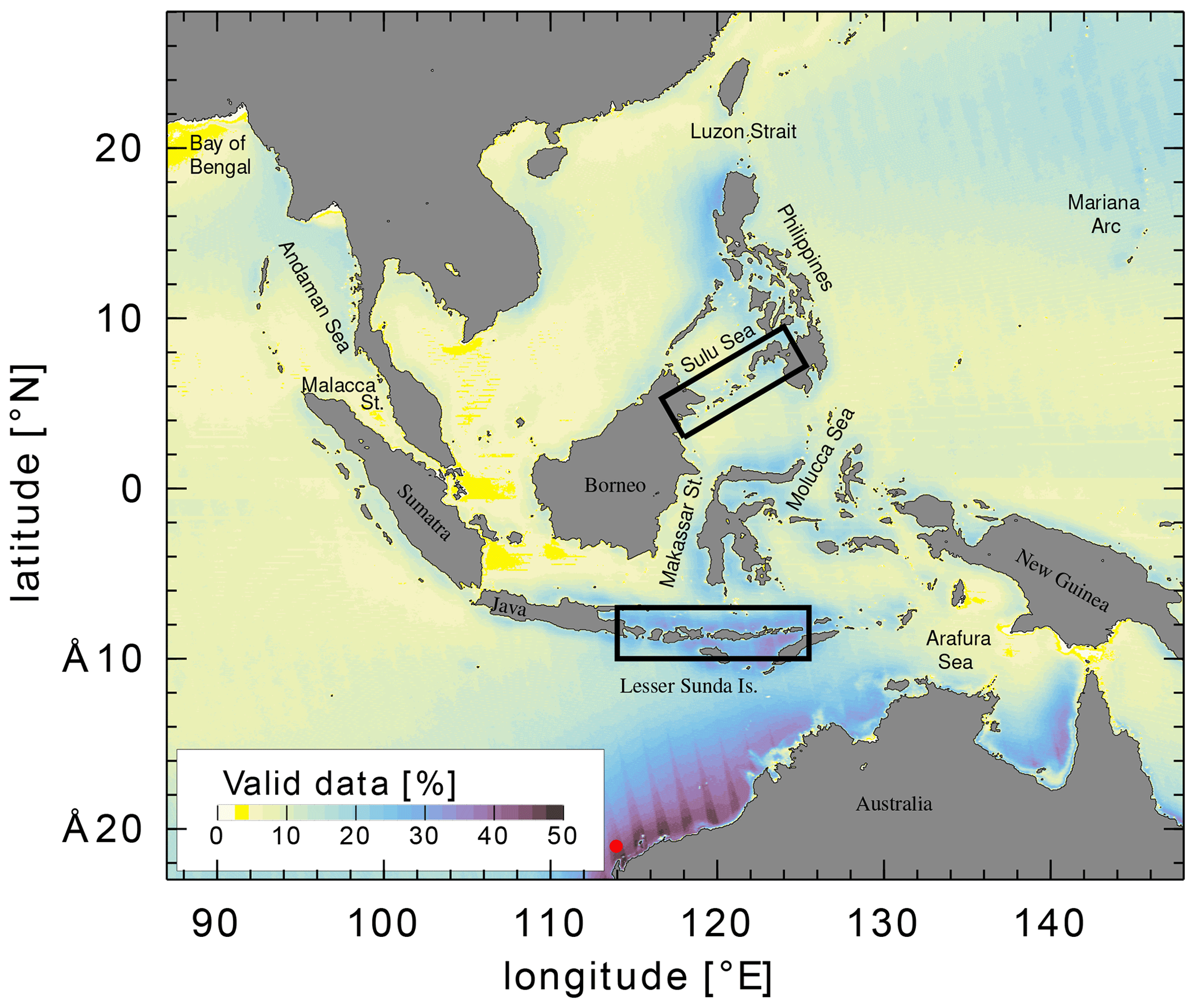
Figure 1 The percentage of valid Chl a observations per pixel in the Level-3 GlobColour daily MODIS product. The rectangular boxes indicate regions enlarged in subsequent figures. The maximum possible observation count, if there were no data gaps, is 7264 for the time period of the observations (July 2002 to August 2022). The red marker at 21^∘ S, 114^∘ E indicates the location of the time series used for Fig. 2.

The choice of frequencies used in the harmonic analysis was informed by previous studies (Susanto et al., 2006; Ray and Susanto, 2016; Xing et al., 2021) and trial and error. Figure 2 shows the power spectrum of Chl a from a region off the northwest coast of Australia. The spectral estimate was computed by averaging the Lomb–Scargle periodogram over overlapping blocks of 60 observations (120 d time series, typically). The spectrum shows a narrowband peak at MS_f, and broadband variability close to the sub- and super-harmonics of this frequency (labeled M_m and 2SM, respectively), superimposed on a red broadband spectrum.

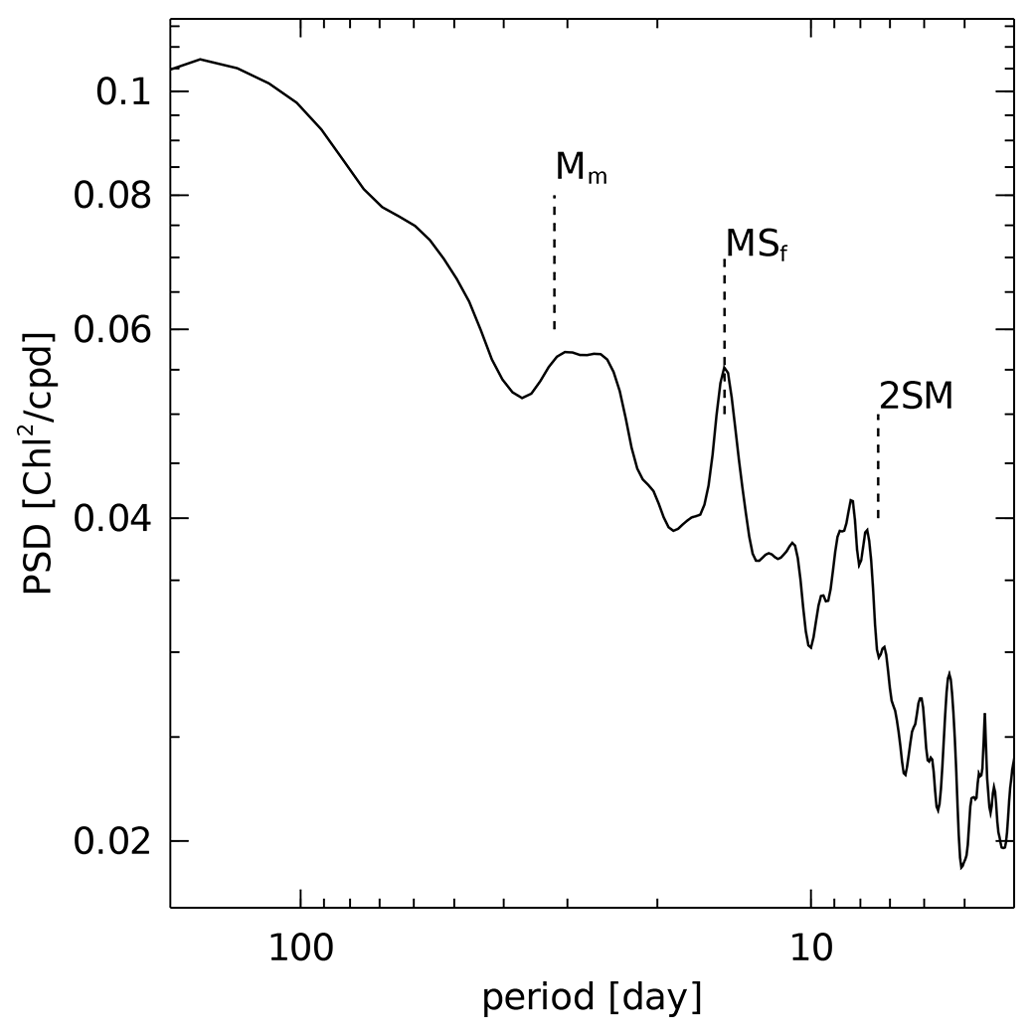
Figure 2 Spectral estimate of Chl a concentration off the northwest coast of Australia (21^∘ S, 114^∘ E). The spectral estimate is computed by averaging Lomb–Scargle periodograms based on Hamming-windowed data within 120 d segments. A narrow peak is evident at the MS_f frequency (corresponding to 14.77 d, the M₂–S₂ spring–neap cycle), and broadband variance is present close to the first sub- and super-harmonics of MS_f (denoted M_m and 2SM). Harmonic analysis at the M_m and 2SM frequencies, and at nearby compound overtide frequencies, did not find significant amplitude.

The choice of harmonic analysis' frequencies was also guided by experiments with analysis at the frequencies of S_a (the annual period), S_sa (the semi-annual period), M_m, MS_f, 2SM, and the annual modulates of MS_f. Based on comparison of the harmonic constants with the estimated standard error and bias errors discussed in the Appendix, only the signals at the S_a and MS_f frequencies were of unambiguous significance. Thus, the plots below are restricted to the results for the S_a and MS_f variability. Experiments with harmonic analysis of log ₁₀(Chl a) were conducted, but these did not reveal relevant differences in the goodness of fit or significance compared to Chl a, so the latter is shown below.

The least-squares harmonic analysis of Chl a was conducted using standard methods (Foreman et al., 2009). At each pixel a time series of Chl a was assembled, y, and the design matrix, A, was constructed with columns consisting of a constant (mean) and the cosine and sine of the astronomical arguments for the annual (S_a, Doodson number 0 565 555) and lunisolar fortnightly (MS_f, Doodson number 0 735 555) cycles. The vector of in-phase and quadrature harmonic constants, x, was obtained as the least-squares solution of the linear system y=Ax.

Missing data in the ocean color observations are largely attributable to clouds. Because the clouds are associated with changes in weather related to the quasi-periodic monsoon cycle, there is concern that the Chl a harmonic constants could be biased by the correlations of data gaps with Chl a variability. To examine this possibility, a simulation study was conducted using a gap-free time series, namely, reanalysis winds from this region, as described in the Appendix. It was found that bias errors on the scale of 10 % to 20 % may be expected in the estimated mean and annual cycles of Chl a over much of the domain. In contrast, the S_sa variability is strongly influenced by data gaps, and for this reason it is not shown. The data gaps can also cause significant error in MS_f estimates due to crosstalk from the larger-amplitude low frequencies. Therefore, MS_f estimates are not shown where they are smaller than 10 % of the mean Chl a. The reader is referred to the Appendix for a detailed analysis.

In addition to the systematic error due to data gaps, it is necessary to quantify the random error related to measurement noise and non-tidal variability. Due to data gaps, the standard least-squares estimate computed from the spectrum of the residual is not applicable. Instead, the method of Matte et al. (2013) is used, which is equivalent to the standard approach in the limit of gap-free data. The method uses the unitary discrete Fourier transform, denoted with matrix F, to estimate a pseudo-spectrum of the residual. Given the residual, $\mathit{r}=\mathit{y}-\mathbf{A}\mathit{x}$, a pseudo-spectrum of r is defined as $S\left(\mathit{r}\right)=\mathbf{F}\mathit{r}\cdot (\mathbf{F}\mathit{r}{)}^{*}$, where ⋅ denotes the element-wise Schur product and superscript * denotes the complex conjugate. S(r) is referred to as a pseudo-spectrum because it is computed from unevenly spaced data; however, it is equal to the periodogram in the case of an evenly spaced (gap-free) time series. After smoothing S(r) to make the pseudo-spectrum continuous, the error variance of x is computed with a Monte Carlo estimate of the matrix: ${\mathbf{A}}^{-\mathrm{1}}{\mathbf{F}}^{\mathrm{T}}\mathrm{diag}\left(S\right(\mathit{r}\left)\right){\mathbf{FA}}^{-\mathrm{1}}$. This error estimate assumes that the covariance of the Fourier transform of the residual, Fr, is diagonal, i.e., that the noise in r is uncorrelated between pseudo-frequencies. This error estimate was compared to an approach mentioned in Ray and Susanto (2016), wherein the noise of the tidal harmonic constants was estimated by comparing it with the amplitude estimated at “fake” tidal frequencies and found to agree well. The fake frequencies used were S_a plus one cycle per 9 years (Doodson number 0 567 555) and MS_f minus three cycles per year (Doodson number 0 205 555). In the plots shown below, the amplitude and phase of the Chl a harmonic constants are only plotted if the amplitude exceeds twice the estimated error level.

3 Results

Figure 3 shows the results of harmonic analysis for the mean Chl a concentration and the S_a and MS_f signals. Comparing the mean and S_a (panels a and b), it is evident that the seasonal variation of Chl a is nearly 50 % of the mean in many coastal areas, specifically, in the northeast Bay of Bengal, in the northeast Andaman Sea, in the northeast Arafura Sea, and along the southern coast of Java. In contrast, the significant MS_f variability of Chl a is largely restricted to a few distinct sites and regions (panel d), including the northwest Australian shelf, the southern part of the Sulu Sea, between the Lesser Sunda Islands, at sites in the Molucca Sea, and in a few other coastal areas. Two of these regions are enlarged in Figs. 4 and 5, below.

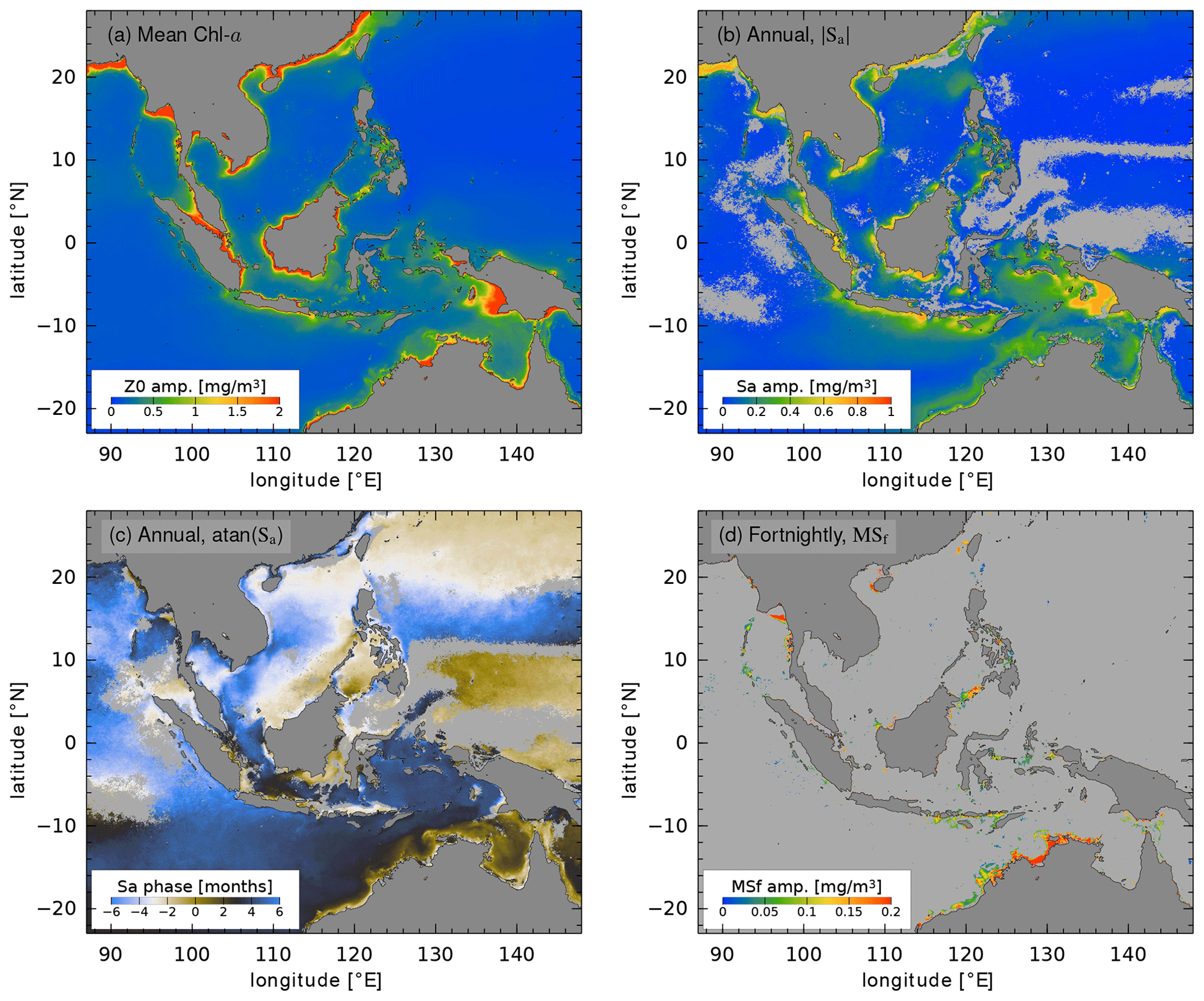
Figure 3 Results of harmonic analysis of Chl a concentration: (a) mean, (b) amplitude of annual cycle (S_a), (c) phase of S_a, measured relative to the vernal equinox (20 March; brown corresponds to a maximum in February–April, black to May–July, blue to August–October, and white to November–January), and (d) amplitude of the fortnightly cycle (MS_f). Two shades of gray are used to indicate land (dark gray) and non-significant amplitude compared to the noise estimate (light gray). Note the different color scale used in each panel.

Throughout the deep ocean, where its amplitude is small, S_a is characterized by a smoothly varying phase associated with the winter season poleward of about 20^∘ latitude in both hemispheres (Fig. 3c). Equatorward of 20^∘, the annual cycle peaks in June–September (Northern Hemisphere summer) throughout much of the Indonesian seas (Susanto et al., 2006); however, strong spatial gradients are associated with the northwest Australian shelf and other coastal areas. The seasonal cycle peaks earlier in the year (January–February) near the island of Borneo, in the Sulu Sea, and further eastward in the Pacific. The relationship between monsoonal and low-frequency variability of Chl a is described in detail in Mandal et al. (2021), Wirasatriya et al. (2021), and Mandal et al. (2022).

Enlarged maps of the MS_f amplitude and phase around the Sulu Archipelago are shown in Fig. 4 (region indicated in Fig. 1). The largest amplitudes are found in the southern Sulu Sea (on the north side of the archipelago), in an area known for its large-amplitude tidal internal waves (Apel et al., 1985; Zhang et al., 2020; Zhao et al., 2021). The peak amplitude of MS_f, 0.2 mg m⁻³, is about one-quarter as large as the mean here, so it represents a significant modulation of the Chl a concentration. The region of maximum MS_f amplitude is associated with a phase lag which varies from about 7 d in the east (x=100 km) to 10 d (i.e., equivalent to −4 d on the color scale) in the west ($x=-\mathrm{100}$ km). The phase is measured relative to the tidal potential, but Ray and Susanto (2016) show that the barotropic semidiurnal tide at this location lags the potential by about 1.2 d. Thus, the fortnightly maximum in Chl a occurs from about 6 to 9 d after the maximum spring–neap tides in this region.

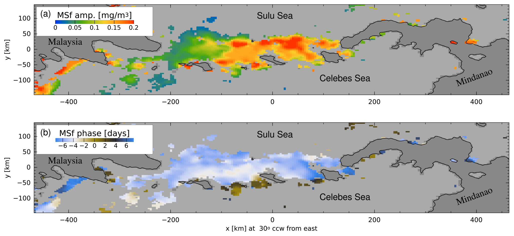
Figure 4 (a) Amplitude and (b) phase of the fortnightly MS_f harmonic constants of Chl a along the Sulu Archipelago (indicated in Fig. 1).

Figure 5 shows MS_f Chl a in the area around the Lesser Sunda Islands, from Bali to Ombai Strait. The maximum in Chl a occurs between the islands of Lombok and Sumbawa in the west and within the northern part of the Ombai Strait in the east. The phase lag exhibits a relatively strong southward gradient, but close to the islands it is about 8 d lagged from the astronomical potential. The barotropic tide lags the potential by about 2 d here (Ray and Susanto, 2016), so the fortnightly Chl a maximum again lags the spring tides by about 6 d. The phase propagates southward at a rate of roughly 5 d per 80 km, equivalent to 0.2 m s⁻¹.

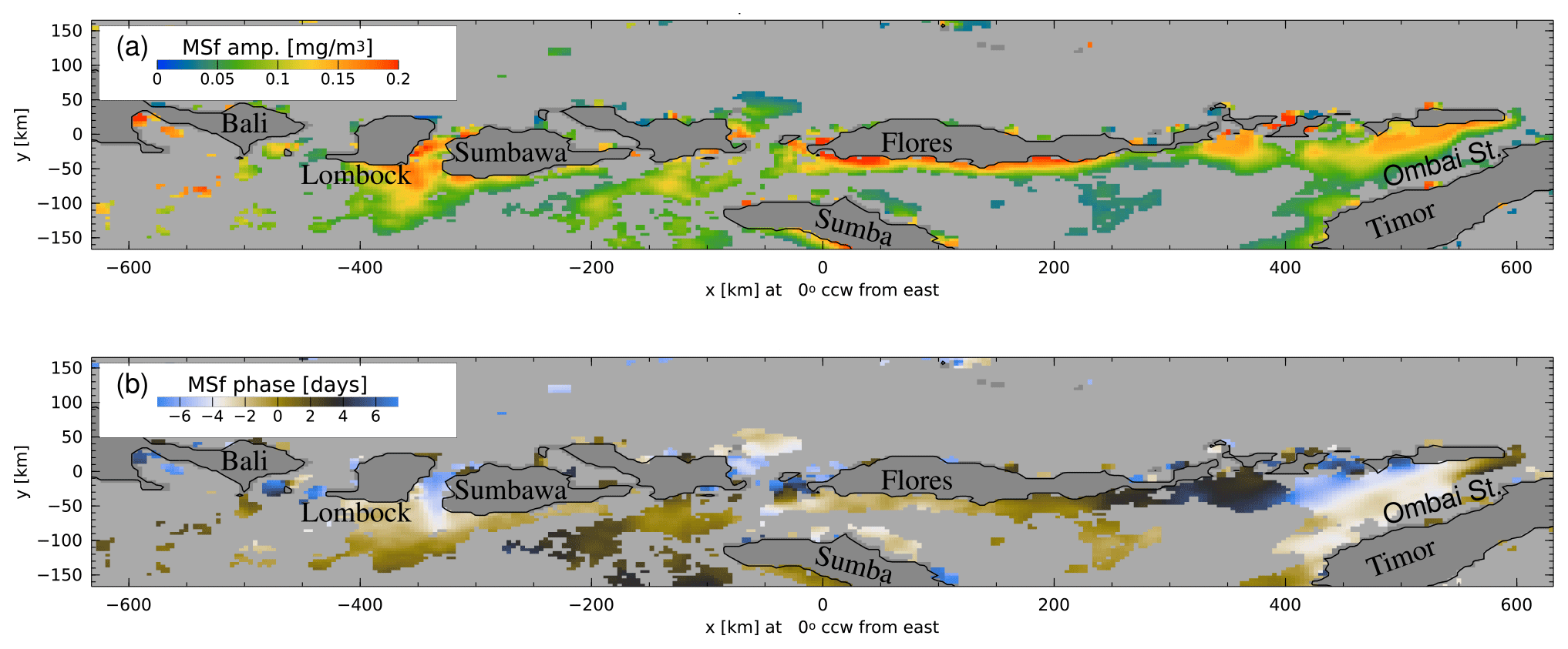
Figure 5 (a) Amplitude and (b) phase of the fortnightly MS_f harmonic constants of Chl a along the Lesser Sunda Islands, from Bali to Ombai Strait (indicated in Fig. 1).

4 Discussion

The mean and annual variability of Chl a shown above replicates the results of Susanto et al. (2006), providing an update with greater resolution based on the longer time series and different satellite missions now available. The use of harmonic analysis to explicitly separate the mean, annual, and fortnightly variability represents an alternative to the climatologies averaged into calendar months or lunar phase used in previous works (Susanto et al., 2006; Shi et al., 2011). The harmonic analysis of Chl a, together with its error estimate, appears to provide more reliable classification of significant and non-significant signals, for example, as compared with the wavelet-based approach of Xing et al. (2021), which indicated significant MS_f variability in relatively large regions of the deep Indian and Pacific oceans.

The fortnightly maximum of Chl a lags the spring tide by roughly 6 to 9 d for the examples cited previously in the southern Sulu Sea and along the Lesser Sunda Islands, and roughly the same phase lag occurs at other sites along the northwest Australian shelf and along the archipelagos in the Molucca Sea. The Chl a phase lag thus exceeds the 1 to 3 d lag between the spring tide and the SST minimum estimated by Ray and Susanto (2016). The potential relationship between Chl a and nutrient inputs due to tidal mixing is complex (Laws, 2013), but the timing of the fortnightly Chl a maximum is logically consistent with the co-occurrence of vertical nutrient and heat fluxes associated with tidal mixing, leading to a productivity maximum and Chl a peak a few days later.

In some respects the spatial distribution of MS_f Chl a variability coincides with the map of sub-surface tidal dissipation inferred in the numerical model of Nugroho et al. (2018) (their Fig. 7), but it is notable that the MS_f Chl a signal is absent in many regions where the dissipation is large, e.g., in the Strait of Malacca, in the Makassar Strait, and in the northern Arafura Sea.

Figure 6 Diagnostics of the barotropic tidal currents, based on the TPXO9-Atlas tide model (Egbert and Erofeeva, 2002). (a) The amplitude of the combined M₂–S₂ current at the MS_f period. Solid contours show the coastline and 50, 200, and 2000 m isobaths. (b) The amplitude of the vertical particle displacement due to the combined M₂–S₂ bottom flow across isobaths.

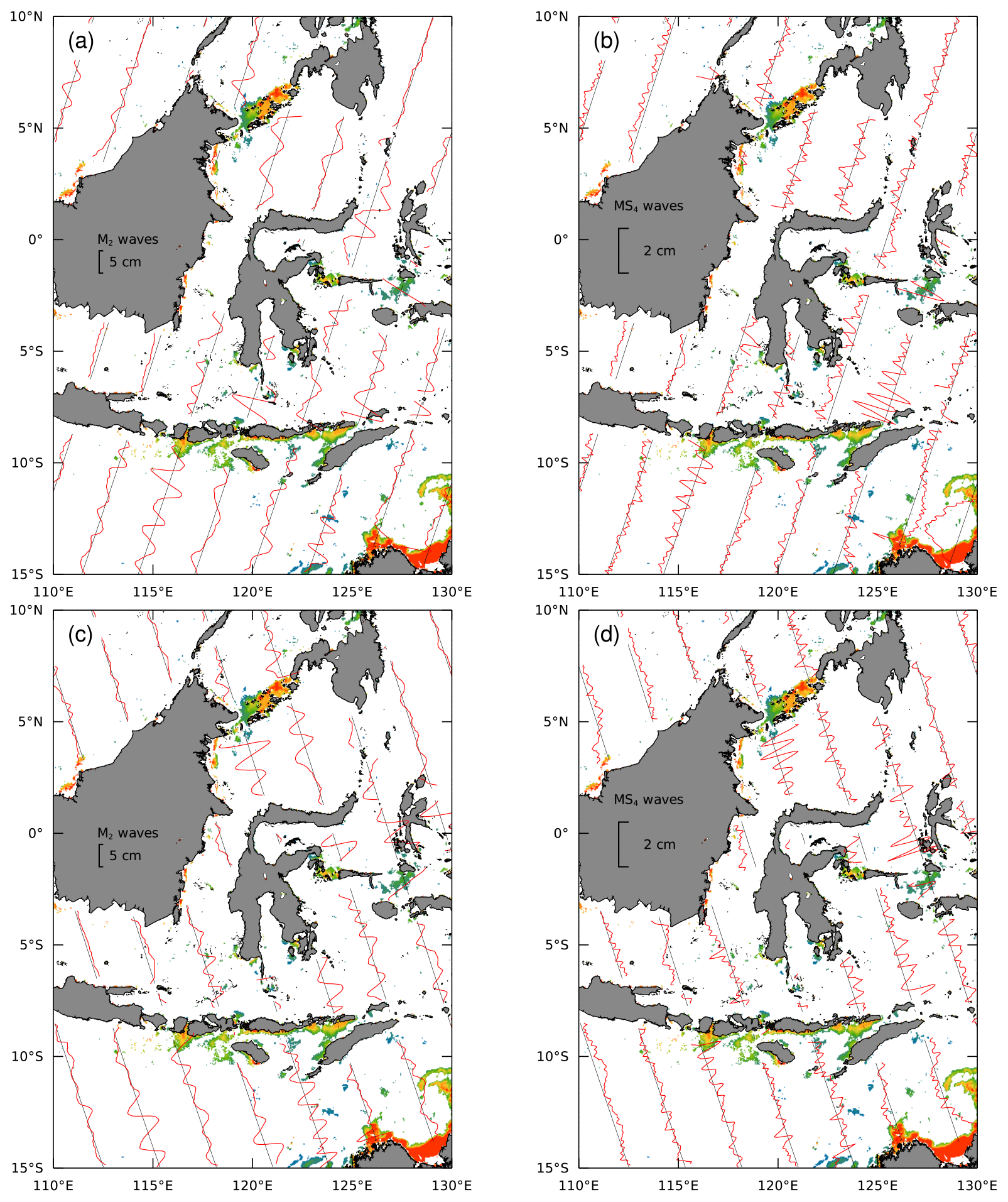
Figure 7 Harmonic analysis of along-track altimeter data. Panels (a) and (c) show sea level anomaly associated with the M₂ astronomical tide. Panels (b) and (d) show sea level anomaly associated with the MS₄ nonlinear overtide. Ascending and descending orbit ground tracks are shown in the upper and lower panels, respectively. The background image is reproduced enlarged from Fig. 3d, with gray values plotted in white for clarity.

In order to understand the mechanisms of Chl a variability, Fig. 6 illustrates two diagnostics computed from the barotropic currents predicted by the TPXO9 tidal model (Egbert and Erofeeva, 2002). The first diagnostic is denoted ΔU, and it is the barotropic tidal current speed associated with the spring–neap cycle (Fig. 6a). Assuming that the energy source that drives the fortnightly mixing is proportional to the kinetic energy (KE) of the combined M₂ and S₂ tides,

$$\begin{array}{}\text{(1)}& \mathrm{KE}={\displaystyle \frac{\mathrm{1}}{\mathrm{2}}}\left(U_{\mathrm{1}}\cos \right({\mathit{\omega }}_{\mathrm{1}}t-{\mathit{\varphi }}_{\mathrm{1}})+U_{\mathrm{2}}\cos ({\mathit{\omega }}_{\mathrm{2}}t-{\mathit{\varphi }}_{\mathrm{2}}){)}^{\mathrm{2}},\end{array}$$

where U_i is the major axis of the tidal current, ω_i is the frequency, ϕ_i is the phase lag, and subscripts 1 and 2 correspond to the M₂ and S₂ tides, respectively, then the amplitude of the spring–neap cycle of KE is given by the product (ΔU)²=U₁U₂. In contrast, the baroclinic tide is generated by flow across topography, leading to localized vertical displacements of isopycnals and baroclinic pressure gradients. A metric of this quantity is $\mathrm{\Delta }Z=w/{\mathit{\omega }}_{\mathrm{1}}$, the vertical displacement of a water parcel flowing along the bottom (Fig. 6b), where $w=|w_{\mathrm{1}}{w}_{\mathrm{2}}{|}^{\mathrm{1}/\mathrm{2}}$ is given in terms of the cross-isobath M₂ and S₂ currents, $w_i=-{\mathit{u}}_i\mathrm{\nabla }H$, with u_i the major-axis current vector.

Figure 6a shows that ΔU is greatly enhanced in several areas where the amplitude of Chl a MS_f is large, especially along the northwest Australian shelf and in the Gulf of Martaban at the north end of the Andaman Sea. In contrast, Fig. 6b shows that large values of ΔZ coincide with large-amplitude MS_f Chl a along the Lesser Sunda Islands and across sills adjacent to the Molucca and Sulu seas. Just as with the Nugroho et al. (2018) dissipation estimate, it is also notable that there are a number of sites where ΔZ is large, among the Andaman–Nicobar Islands and within Luzon Strait, where the MS_f Chl a amplitude is not significant. Indeed many of these same regions are well-known for the presence of nonlinear internal waves (Osborne and Burch, 1980; Zhao and Alford, 2006), and it is puzzling that a robust MS_f Chl a signal is not detected at these sites.

A more direct view of baroclinic tidal processes in the region is provided by satellite altimetry (Fig. 7). The nearly 30-year record of data along the TOPEX/Jason ground tracks is long enough that the sea level anomaly phase-locked with the astronomical tide can be identified with sub-centimeter precision (Zaron, 2019). Figure 7a and c illustrate that the M₂ sea level anomaly in some places exceeds 5 cm (south of Lombok in Fig. 7a and in the western Celebes Sea in Fig. 7c), which is evidence of the strong and localized baroclinic tidal generation in this region. Figure 7b and d show the presence of small but clearly identifiable waves at the MS₄ overtide frequency in the same locations just noted, as well as north of Ombai Strait, in the western Sulu Sea (Fig. 7b), in the Molucca Sea, and in the eastern Banda Sea (Fig. 7d). These waves at the MS₄ frequency represent the high-frequency counterpart of the nonlinearity which should also manifest at the MS_f frequency.

Although the altimeter ground tracks are spaced too far apart to map the MS₄ waves in two dimensions, their along-track wavelength is consistent with the interpretation that they are mode-1 internal waves (59 to 66 km, based on the World Ocean Atlas stratification; Zaron et al., 2022). The decay of the waves southward from Lombok, northward from Ombai, and southward from the Sulu Archipelago clearly implicates narrow passages between the islands as their sites of genesis.

We hypothesize that the fortnightly modulation of surface Chl a identified from ocean color is the result of tidally driven mixing, which supports a fortnightly modulation of the vertical nutrient transport. The locations with significant fortnightly Chl a variability, aside from the northwest shelf of Australian and the northern Andaman Sea, nearly all coincide with regions where strong fortnightly modulation of the cross-isobath flow is expected to occur (Fig. 6b). There is evidence for nonlinear interactions at a subset of these sites, from sparse altimetry, at the sum of the M₂ and S₂ frequencies (Fig. 7b and d).

Fieldwork would be required to assess the validity of this hypothesis, since it presupposes the existence of a nutrient-limited standing stock of phytoplankton capable of assimilating the periodic influx of nutrients, a vertical nutrient gradient, and a marginally stable water column susceptible to destabilization by tidal currents. Among the high-resolution tide-resolving numerical models of the Indonesian seas (e.g., Robertson and Ffield, 2008; Nagai and Hibiya, 2015; Hermansyah et al., 2019), the MS₄ overtides have not been specifically studied, but the altimeter-derived estimates for this tide could be used to validate the nonlinear dynamics resolved in these models. One plausible mechanism for tidally induced mixing involves near-bottom overturning initiated where cross-isobath particle displacement is comparable to the vertical motion of the linear internal tide (Levine and Boyd, 2006; Klymak et al., 2008). Another mechanism, which would lead to mixing higher in the water column, is the convective instability of the massive internal waves which have been observed in locations of strong tidal currents in this region (Atmadipoera and Suteja, 2018; Bouruet-Aubertot et al., 2018).

5 Conclusions

Harmonic analysis has been conducted of 20 years of daily MODIS-Aqua-derived Chl a measurements to identify regions of tidal influence on biological production in the Indonesian seas and the nearby Indian and Pacific oceans. The choice of analysis frequencies, S_a and MS_f, was dictated by the spectral resolution feasible with the time series, which suffer from extensive gaps due to clouds. The results agree with previous estimates of S_a (Susanto et al., 2006) and reveal several sites and regions where the Chl a concentration is phase-locked with the spring–neap cycle, peaking around 6 to 9 d after the local maximum of tidal currents.

The locations of the largest MS_f signals, off the northwest coast of Australia and in the vicinity of narrow channels between islands, generally correspond to regions where boundary-layer-driven and internal wave-driven mixing are expected to occur, based on comparisons with models. However, there are a number of regions where tidal dissipation is large or where large-amplitude internal waves are well-known but where a significant MS_f Chl a amplitude is not found. This observation highlights the obvious point that tidal controls on Chl a occur only at sites where the environmental prerequisites for such control are suitable.

One limitation of the present estimates is the difficulty of identifying the small MS_f Chl a signal from the gappy data. Experiments to improve the estimates were conducted using spatially coupled harmonic analysis (not shown); however, results were found to be overly sensitive to details of the spatial basis functions used. Ocean models with the capability of simulating the tidal–biological interactions are now being implemented (e.g., Gutknecht et al., 2016), and it may be fruitful to use the surface Chl a fields from these models as spatial basis functions within a spatially coupled harmonic analysis, as was recently done for sea-surface-height data (Egbert and Erofeeva, 2021). While imperfect, such an approach may provide the capability to utilize the gappy data more effectively to map periodic components of the Chl a fields.

Appendix A: The impact of data gaps on harmonic analysis

Building on the notation of the main text, consider a data indicator vector, w, the same size as the data vector, y, with entries 0 or 1 depending on whether the data value is valid (i.e., used in the harmonic analysis) or invalid (i.e., omitted as part of a data gap), respectively. Define the rectangular diagonal matrix, $\widehat{\mathbf{W}}$, which maps from the original data vector, y, to the gappy data vector by picking out those entries which correspond to nonzero entries in the w vector. Given the data vector, y, the corresponding gappy data vector shall be denoted $\widehat{\mathit{y}}=\widehat{\mathbf{W}}\mathit{y}$, and the design matrix for the harmonic analysis of the gappy data shall be denoted $\widehat{\mathbf{A}}=\widehat{\mathbf{W}}\mathbf{A}$. For convenience, define the square diagonal weighting matrix, $\mathbf{W}={\widehat{\mathbf{W}}}^{\mathrm{T}}\widehat{\mathbf{W}}$, which contains the elements of w along its diagonal. Finally, let ${\mathbf{W}}_{\mathrm{c}}=\mathbf{I}-\mathbf{W}$ denote the complement of the weight matrix with diagonal w_c, where ${\mathit{w}}_{\mathrm{c}}=\mathbf{1}-\mathit{w}$ is the complement of the data indicator vector.

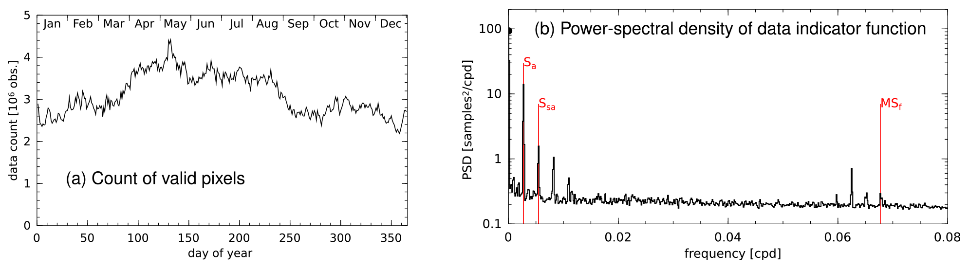
Figure A1 (a) The count of good data, i.e., cloud-free pixels, exhibits a notable annual cycle associated with monsoon variability. Data counts are about 30 % greater during the dry season than during the monsoon season (roughly September through March). (b) The power spectral density of the data indicator function, w, contains significant peaks at the frequency of the annual cycle (S_a) and its harmonics (the semi-annual cycle, S_sa, is indicated). A peak at the fortnightly frequency (MS_f) is present, but it is almost 3 orders of magnitude smaller than the peak at the zero frequency (98 samples² cpd⁻¹ (cpd – cycles per day), marked with a dot). The spectrum is computed by averaging the Hamming-windowed periodograms computed from data indicator time series at each ocean pixel.

With the above extensions of the original notation, it is possible to approximately compute the sensitivity of the harmonic constants to the data gaps. The harmonic constants based on the gappy data are given by

$$\begin{array}{}\text{(A1)}& {\displaystyle }\widehat{\mathit{x}}& {\displaystyle }=({\widehat{\mathbf{A}}}^{\mathrm{T}}\widehat{\mathbf{A}}{)}^{-\mathrm{1}}{\widehat{\mathbf{A}}}^{\mathrm{T}}\widehat{\mathit{y}},\text{(A2)}& {\displaystyle }& {\displaystyle }=({\mathbf{A}}^{\mathrm{T}}\mathbf{WA}{)}^{-\mathrm{1}}{\mathbf{A}}^{\mathrm{T}}\mathbf{W}\mathit{y},\text{(A3)}& {\displaystyle }& {\displaystyle }=\left({\mathbf{A}}^{\mathrm{T}}\right(\mathbf{I}-{\mathbf{W}}_{\mathrm{c}}\left)\mathbf{A}{)}^{-\mathrm{1}}{\mathbf{A}}^{\mathrm{T}}\right(\mathbf{I}-{\mathbf{W}}_{\mathrm{c}})\mathit{y}.\end{array}$$

A Neumann series can be used to approximate the inverse, above, in terms of powers of W_c:

$$\begin{array}{}\text{(A4)}& {\displaystyle }& {\displaystyle }\left({\mathbf{A}}^{\mathrm{T}}\right(\mathbf{I}-{\mathbf{W}}_{\mathrm{c}})\mathbf{A}{)}^{-\mathrm{1}}=({\mathbf{A}}^{\mathrm{T}}\mathbf{A}-{\mathbf{A}}^{\mathrm{T}}{\mathbf{W}}_{\mathrm{c}}\mathbf{A}{)}^{-\mathrm{1}},\text{(A5)}& {\displaystyle }& {\displaystyle }=\left[\right({\mathbf{A}}^{\mathrm{T}}\mathbf{A}\left)\right(\mathbf{I}-\left({\mathbf{A}}^{\mathrm{T}}\mathbf{A}{)}^{-\mathrm{1}}{\mathbf{A}}^{\mathrm{T}}{\mathbf{W}}_{\mathrm{c}}\mathbf{A}\right){]}^{-\mathrm{1}},\text{(A6)}& {\displaystyle }& {\displaystyle }=(\mathbf{I}+({\mathbf{A}}^{\mathrm{T}}\mathbf{A}{)}^{-\mathrm{1}}{\mathbf{A}}^{\mathrm{T}}{\mathbf{W}}_{\mathrm{c}}\mathbf{A}+\mathrm{\dots }\left)\right({\mathbf{A}}^{\mathrm{T}}\mathbf{A}{)}^{-\mathrm{1}},\end{array}$$

where the dots denote quadratic and higher-order terms in W_c. Substituting this approximation in Eq. (A3), one obtains

$$\begin{array}{}\text{(A7)}& {\displaystyle }\begin{array}{rl}& \widehat{\mathit{x}}=(\mathbf{I}+({\mathbf{A}}^{\mathrm{T}}\mathbf{A}{)}^{-\mathrm{1}}{\mathbf{A}}^{\mathrm{T}}{\mathbf{W}}_{\mathrm{c}}\mathbf{A}+\mathrm{\dots }\left)\right({\mathbf{A}}^{\mathrm{T}}\mathbf{A}{)}^{-\mathrm{1}}\\ & \cdot {\mathbf{A}}^{\mathrm{T}}(\mathbf{I}-{\mathbf{W}}_{\mathrm{c}})\mathit{y},\end{array}\text{(A8)}& {\displaystyle }\begin{array}{rl}& =\left({\mathbf{A}}^{\mathrm{T}}\mathbf{A}{)}^{-\mathrm{1}}{\mathbf{A}}^{\mathrm{T}}\right(\mathbf{I}-{\mathbf{W}}_{\mathrm{c}})\mathit{y}+({\mathbf{A}}^{\mathrm{T}}\mathbf{A}{)}^{-\mathrm{1}}{\mathbf{A}}^{\mathrm{T}}\\ & \cdot {\mathbf{W}}_{\mathrm{c}}\mathbf{A}\left({\mathbf{A}}^{\mathrm{T}}\mathbf{A}{)}^{-\mathrm{1}}{\mathbf{A}}^{\mathrm{T}}\right(\mathbf{I}-{\mathbf{W}}_{\mathrm{c}})\mathit{y}+\mathrm{\dots },\end{array}\text{(A9)}& {\displaystyle }\begin{array}{rl}& =\mathit{x}-({\mathbf{A}}^{\mathrm{T}}\mathbf{A}{)}^{-\mathrm{1}}{\mathbf{A}}^{\mathrm{T}}{\mathbf{W}}_{\mathrm{c}}\mathit{y}+({\mathbf{A}}^{\mathrm{T}}\mathbf{A}{)}^{-\mathrm{1}}{\mathbf{A}}^{\mathrm{T}}\\ & \cdot {\mathbf{W}}_{\mathrm{c}}\mathbf{A}({\mathbf{A}}^{\mathrm{T}}\mathbf{A}{)}^{-\mathrm{1}}{\mathbf{A}}^{\mathrm{T}}\mathit{y}+\mathrm{\dots },\end{array}\text{(A10)}& {\displaystyle }\begin{array}{rl}& =\mathit{x}-\left({\mathbf{A}}^{\mathrm{T}}\mathbf{A}{)}^{-\mathrm{1}}{\mathbf{A}}^{\mathrm{T}}{\mathbf{W}}_{\mathrm{c}}\right(\mathit{y}-\mathbf{A}\left({\mathbf{A}}^{\mathrm{T}}\mathbf{A}{)}^{-\mathrm{1}}{\mathbf{A}}^{\mathrm{T}}\mathit{y}\right)\\ & +\mathrm{\dots },\end{array}\text{(A11)}& {\displaystyle }\widehat{\mathit{x}}-\mathit{x}=-\left({\mathbf{A}}^{\mathrm{T}}\mathbf{A}{)}^{-\mathrm{1}}{\mathbf{A}}^{\mathrm{T}}{\mathbf{W}}_{\mathrm{c}}\right(\mathit{y}-\mathbf{A}\mathit{x})+\mathrm{\dots },\end{array}$$

Note that y−Ax is the residual, r, data minus predicted signal, obtained from the harmonic analysis of the gap-free data.

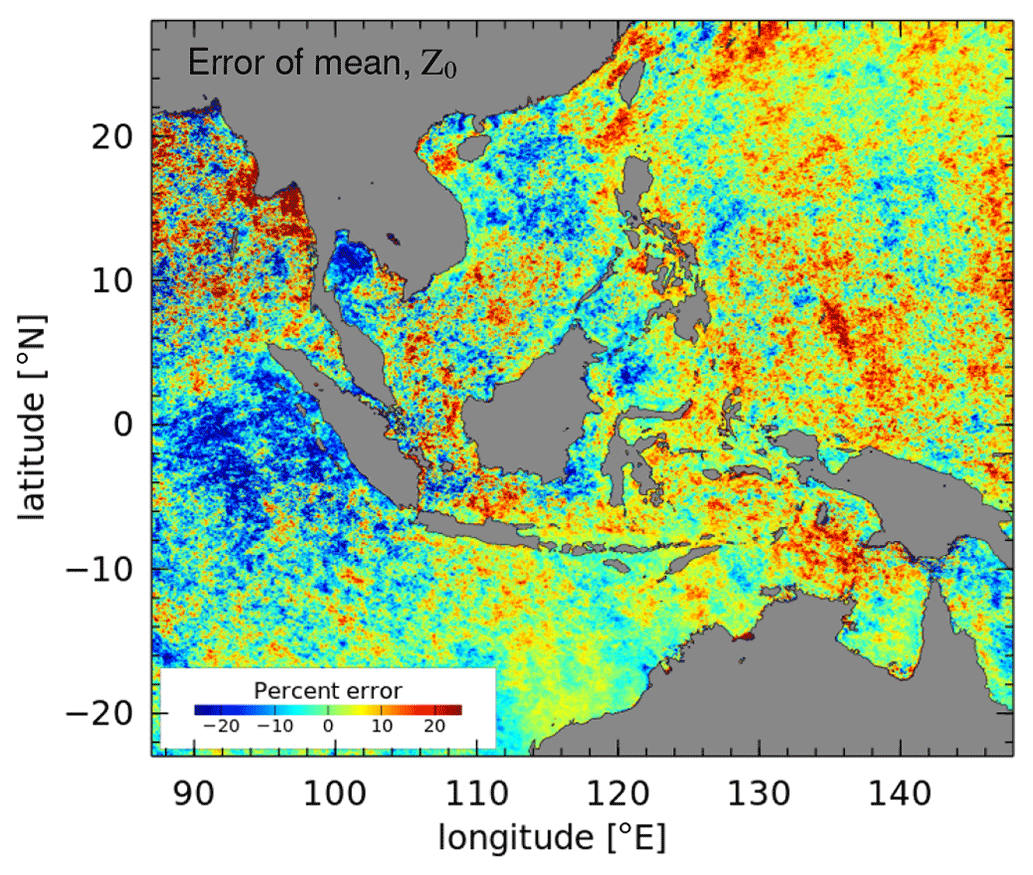
Figure A2 The relative error in the estimated mean (Z₀) of the meridional wind shows the effect of Chl a data gaps at each pixel. For this example, the time series of the NCEP reanalysis 850 mbar meridional wind at 7.5^∘ S, 110^∘ E is taken as the reference gap-free “truth”, and the mean is compared with the mean estimated from the gappy time series at each oceanic pixel, according to the Chl a data indicator. The error is a measure of the crosstalk of non-sinusoidal (broadband) variability near the S_a frequency which is aliased back to the mean by the gappy sampling. This map shows where data gaps caused by cloudiness are likely to bias the mean estimated for Chl a.

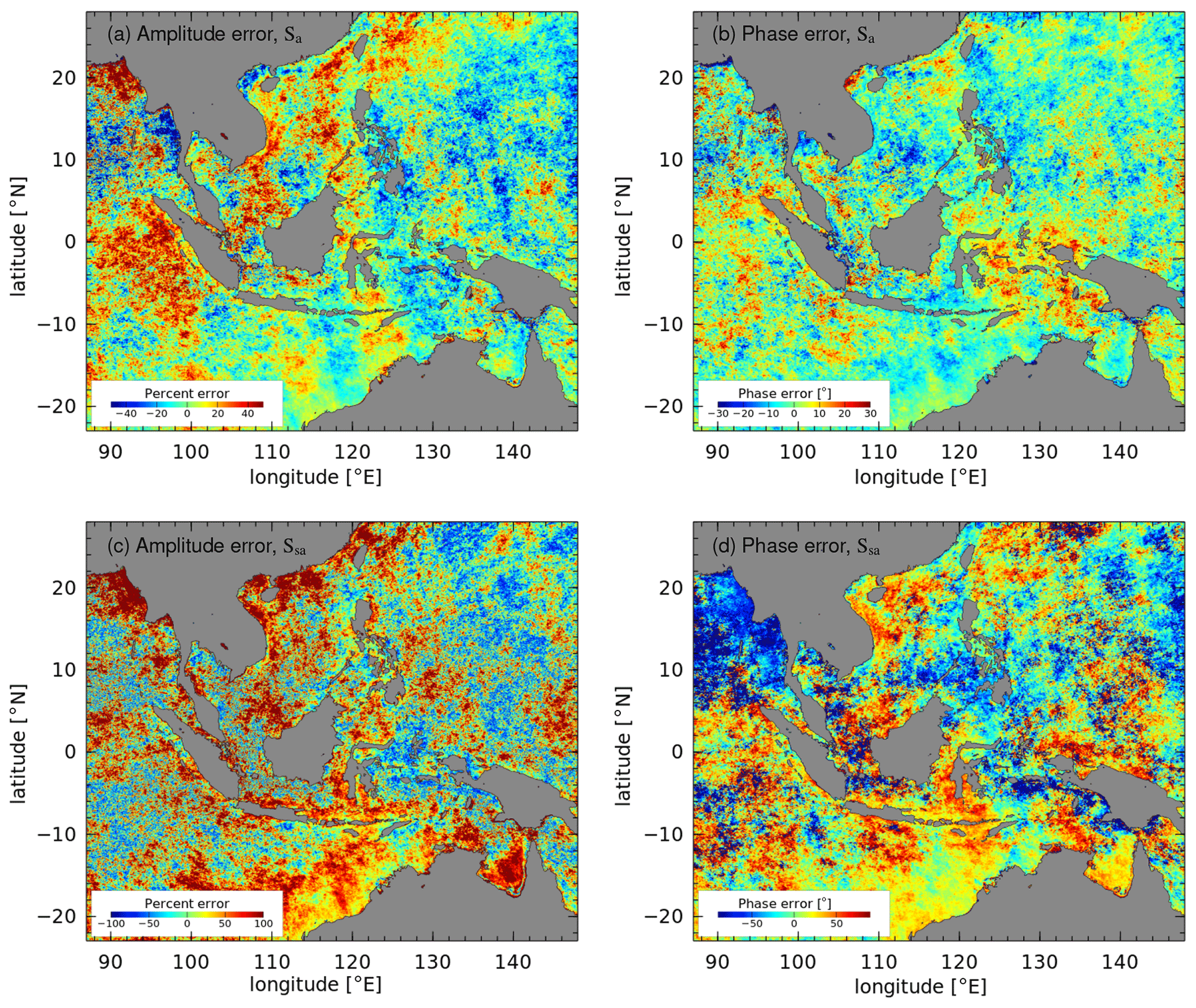
Figure A3 The relative error due to data gaps in amplitude and phase for the harmonic constants at the S_a (a, b) and S_sa (c, d) frequencies, based on harmonic analysis of a representative time series of NCEP reanalysis meridional winds are shown, similar to Fig. A2. Assuming the low-frequency broadband variability of the wind is similar to Chl a, the S_sa harmonic constants are judged as not reliable and are thus omitted from the presentation in the main text.

Equation (A11) shows that if the gap-free time series is described exactly by the harmonic components (i.e., r=0), then the harmonic constants are insensitive to data gaps. The amplitude and phase of each harmonic component is described by exactly two parameters; therefore, as long as the gaps do not reduce the quantity of data below the number of parameters to be estimated (in which case ${\widehat{\mathbf{A}}}^{\mathrm{T}}\widehat{\mathbf{A}}$ would not be invertible), the harmonic constants are uniquely determined, independent of the gaps.

Of course, with real data, the residual will be nonzero whether or not the time series contains gaps. In this case it is useful to note that W_cr is equal to the element-wise (Schur) product of w_c and r, a time-domain product of the complement of the data-gap indicator and the residual time series. Using the convolution theorem, this time-domain product can be interpreted as a convolution in the frequency domain. The effect of data gaps, then, can be regarded as redistributing variance of the gap-free least-squares residual throughout the frequency domain, according to the Fourier transform of the data indicator function, w.

Figure A1a shows the count of valid data pixels versus the day of year, averaged over the 2002–2022 time period. There is a notable increase in the number of cloud-free pixels from late March through August during the dry season in the region of the northern Australia and Indonesia monsoon (Murakami and Matsumoto, 1994), also called the dry southeast monsoon (Aldrian and Susanto, 2003). Indeed, the power spectrum of w_c averaged over all the grid cells of the Chl a dataset exhibits peaks at the S_a and S_sa periods, the larger of which contains about 15 % as much power as the zeroth frequency (Fig. A1b). The power at the MS_f frequency of the spring–neap cycle is about 0.3 % that at the zeroth frequency. While the latter seems negligible, the expected crosstalk is proportional to the square root of this quantity (about 0.05) and the MS_f amplitude is so much smaller than the mean that this crosstalk could be significant. Thus, as mentioned in the main text, MS_f harmonic constants are considered non-significant and not plotted if they are smaller than 0.1 of the mean Chl a value in a given pixel.

As an aside, the MS_f peak in the data indicator spectrum suggests that the data flagging algorithm is influenced by tides in this region. It is conceivable that fortnightly modulations in SST could affect atmospheric stability and cloudiness (Ray and Susanto, 2019); however, it is also possible that some other process affecting ocean color, such as turbidity, might change the outlier flagging in the GSM algorithm.

The concern that data gaps could lead to errors in the S_a and S_sa harmonic constants is also warranted, but it is difficult to estimate the magnitude of this effect for Chl a since the gap-free residual is unknown. In order to assess the potential crosstalk between these frequencies, we have made harmonic analyses of a known signal, in this case, the vector winds at a location in the Java Sea, where the broadband (non-sinusoidal) signals associated with the monsoon cycle are expected to be reasonably similar to the broadband monsoon signals in Chl a, assuming the latter are largely the result of wind-driven variability. The wind time series is taken from the NCEP reanalysis product (Kanamitsu et al., 2002), so the gap-free time series and its harmonic analysis are available for comparison.

The (gap-free) time series of zonal wind has values of −1.5, 5.2, and 2.2 m s⁻¹ for its mean and amplitudes of the S_a and S_sa harmonic constants, respectively. It thus differs from the Chl a time series in which the mean is about twice as large as the S_a amplitude. In contrast, the (gap-free) meridional wind has values of 0.8, 0.6, and 0.15 m s⁻¹, for the mean, S_a, and S_sa amplitudes, respectively, which are in the same order, by size, as the Chl a harmonic constants. Results from the analysis of the meridional wind component are shown below, since these should be more representative of the errors due to data gaps in Chl a.

Figure A2 shows the relative error in the mean wind due to the data gaps, $({\widehat{x}}_{\mathrm{1}}/x_{\mathrm{1}}-\mathrm{1})\times \mathrm{100}\mathit{\%}$, where ${\widehat{x}}_{\mathrm{1}}$ and x₁ are means estimated from the gappy and gap-free time series, respectively. The typical magnitude of the error, about 15 %, is what could be expected from the crosstalk of the S_a and S_sa signals with the mean. As a consequence of the spatial correlations of the data gaps, the errors are also spatially correlated. The largest errors occur in the northern Gulf of Thailand, in the northern Andaman Sea, and near the coastline in the Bay of Bengal. The relative sizes of the S_a and S_sa amplitudes compared to the mean are smaller for Chl a than for the wind, so the bias errors in the estimated Chl a mean field are likely to be smaller than shown, but it is nonetheless clear that the errors due to data gaps could be a significant fraction of the mean.

The crosstalk from the mean and S_sa into the S_a signal is illustrated in Fig. A3a and b; note the larger range of color scales compared to Fig. A2. These panels show, again, a geographic pattern with maximal errors in many of the same regions as above. While errors in the phase are not negligible, they are generally small enough and spatially noisy enough that one would not likely misrepresent the seasonal phasing of the signal, assuming the Chl a errors are comparable.

In contrast, Fig. A3c and d indicate that the data gaps are likely to make the S_sa variability of Chl a impossible to interpret. Indeed, an analysis of the formal (random) error in the S_sa harmonic constants suggests that the signal-to-noise ratio is below 1 in about half of the domain (not shown), and Fig. A3c indicates that the systematic bias due to data gaps is likely to be severe. For this reason, the S_sa analysis is not shown in the main text, although the harmonic constants were computed and are available from the authors.

To conclude, this Appendix provides an analysis of the effect of data gaps on the harmonic analysis of Chl a. Because the cloudiness is correlated with the seasonal and semi-annual cycles, it has the potential to create systematic errors in the seasonal variability estimated via harmonic analysis. Because the magnitude of the effect depends on the residual, i.e., on the component of the signal which is not phase-locked with the components included in the harmonic analysis, it is difficult to analyze without a comparable gap-free dataset. The approach taken here has involved the harmonic analysis of a gap-free dataset consisting of reanalysis winds, which should have low-frequency broadband properties similar to that of Chl a. Based on the present analysis, the mean and annual cycles of Chl a are presented in the main text, for comparison with previous works, but the S_sa variability is not shown since it is unlikely to be reliably determined.