Effects of including the adjoint sea ice rheology on estimating Arctic Ocean–sea ice state

The adjoint assimilation method has been applied to coupled ocean and sea ice models for sensitivity studies and Arctic state estimations. However, the accuracy of the adjoint model is degraded by simplifications of the adjoint of the sea ice model, especially the adjoint sea ice rheologies. As part of ongoing developments in coupled ocean and sea ice estimation systems, we incorporate and approximate the adjoint of viscous-plastic sea ice dynamics (adjoint-VP) and compare it with the adjoint of free-drift sea ice dynamics (adjoint-FD) through assimilation experiments. Using the adjoint-VP results in a further cost reduction of 7.9 % in comparison to adjoint-FD, with noticeable improvements in the ocean temperature over the open water and the intermediate layers of the Arctic Ocean. Adjoint-VP adjusts the model input more efficiently than adjoint-FD does by involving different sea ice retreat processes. For instance, adjoint-FD melts the sea ice up to 1.0 m in the marginal seas from May to June by overadjusting air temperature (>8 ^∘C); adjoint-VP reproduces the sea ice retreat with smaller adjustments to the atmospheric state within their prior uncertainty range. These developments of the adjoint model here lay the foundation for further improving Arctic Ocean and sea ice estimations by comprehensively adjusting the initial conditions, atmospheric forcings, and parameters of the model.

1 Introduction

The Arctic Ocean has experienced drastic changes, including rapidly declining sea ice (Comiso et al., 2008; Kwok, 2018), increased inventory of freshwater in the western Arctic (Proshutinsky et al., 2019), enhanced warm inflows from the Pacific Ocean (Woodgate et al., 2012) and the Atlantic Ocean (Polyakov et al., 2017; Quadfasel et al., 1991), and increased ocean primary productivity (AMAP, 2021); it has also been migrating to a new state over the past decades. These changes potentially impact the climate and weather of the Northern Hemisphere (Ma et al., 2022; Overland et al., 2021).

In recent years, progress has been made in satellite techniques (e.g., Kaleschke et al., 2001; Spreen et al., 2008), in situ observations (e.g., Toole and Krishfield, 2016; Morison et al., 2007; Polyakov et al., 2017; Proshutinsky et al., 2009; Schauer et al., 2008), and coupled ocean and sea ice models. However, the lack of extensive Arctic observations, especially direct observations of the state variables and fluxes through the water column, and the deficiencies in the coupled ocean and sea ice model still obscure our understanding of the Arctic sea ice changes and extremes. Accurate predictions of sea ice are therefore limited (e.g., Yang et al., 2020).

To fill the gaps, research groups have applied data assimilation techniques to ingest available observations into coupled ocean and sea ice models. The resulting reanalyses are assumed to have higher accuracy since as the development of models and data assimilation methods progress and the observation numbers increase. Most of Arctic's coupled ocean and sea ice data assimilation and operational forecasting systems use statistical methods such as optimal interpolation (e.g., Lindsay and Zhang, 2006) and ensemble Kalman filters (e.g., Mu et al., 2018; Sakov et al., 2012). The advantage of these statistical methods is that they ensure a local fit to available observations (within prior uncertainties of both model and observations). However, away from the observations and for the unobserved variables, these methods rely on the inaccurate spatial covariance of model states for interpolation. In addition, these algorithms can introduce artificial sink or source terms to the numerical models.

Over recent decades, an adjoint method with a large assimilation window (years to decades) has been developed in the framework of Estimating the Circulation and Climate of the Ocean (ECCO; Heimbach et al., 2019; Stammer et al., 2002; Wunsch and Heimbach, 2007) to create dynamically consistent ocean reanalyses. This method iteratively minimizes a cost function that measures the model–data “distance” by adjusting model input (control variables). The use of an adjoint model (adjoint of the tangent linear approximation of the nonlinear model) as a spatiotemporal interpolator distinguishes this method from the statistical methods. The resulting reanalysis completely follows the model-governing equations without having to consider artificial source or sink terms. However, the qualities of the reanalysis datasets depend on the accuracy of the tangent linear approximation.

Despite the application of the coupled ocean and sea ice adjoint model in sensitivity studies (Heimbach et al., 2010; Kauker et al., 2009; Koldunov et al., 2013) and reanalyses (Fenty and Heimbach, 2013; Koldunov et al., 2017; Lyu et al., 2021b; Nguyen et al., 2021), we have to omit the adjoint of sea ice dynamics (Fenty et al., 2017; Nguyen et al., 2021) or simplify it to the adjoint of a free-drift sea ice model (Koldunov et al., 2017; Lyu et al., 2021b) to ensure numerical stability of the adjoint model. Toyoda et al. (2019) noted that further inclusion of the adjoint of sea ice rheology results in a much weaker evolution of sensitivity to sea ice velocity by O (10²) in the central Arctic Ocean than the adjoint of free-drift sea ice dynamics (adjoint-FD). It is expected that including the adjoint of sea ice rheology could better project the model–data misfits to the control variables and potentially improve the quality of the reanalysis.

In this study, we incorporate and stabilize the adjoint of viscous-plastic sea ice dynamics (adjoint-VP; Hibler, 1979; Zhang and Hibler, 1997), building on prior developments of the coupled ocean and sea ice model and assimilation system (Fenty and Heimbach, 2013; Heimbach et al., 2010; Koldunov et al., 2017; Lyu et al., 2021b). Using the unprecedented sea ice retreat process in 2012 as an example, we evaluate the impacts of using the approximated adjoint of sea ice rheology on estimating the Arctic Ocean, sea ice, and sea ice retreat processes.

The paper is organized as follows. In Sect. 2, we introduce the model configurations and assimilation experiments. We assess the assimilation results in terms of the residual errors in Sect. 3. We examine adjustments of the control variables in Sect. 4 and compare the sea ice retreat process in the assimilation runs in Sect. 5. Section 6 summarizes the results of this study and discusses the potential for a further development of global and Arctic state and parameter estimation systems.

2 Model configuration and experiment setups

2.1 The coupled ocean and sea ice modeling and assimilation system

The data assimilation system is based on the adjoint method in the ECCO framework, using the Massachusetts Institute of Technology general circulation model (MITgcm; Marshall et al., 1997) coupled with the zero-layer dynamic–thermodynamic sea ice model of Hibler (1979). The sea ice dynamics are based on a viscous-plastic sea ice rheology and are solved using a line successive over-relaxation algorithm (Zhang and Rothrock, 2000). The thermodynamic sea ice model includes a prescribed subgrid-scale ice thickness distribution with seven thickness categories. On top of the ice, a diagnostic snow model is applied which modifies the heat flux and surface albedo, as in Zhang and Rothrock (2000). The thermodynamic–dynamic sea ice model simulates changes in sea ice drift (SID), sea ice concentration (SIC), and mean sea ice thickness (in volume per unit area, mean SIT hereinafter). Losch et al. (2010) reformulated the sea ice model on an Arakawa C grid to match the MITgcm oceanic grid and modified the model codes to permit efficient and accurate automatic differentiation. The adjoint of the coupled ocean and sea ice model is generated by the Transformation of Algorithms (TAF) in FORTRAN (Giering and Kaminski, 1998).

The pan-Arctic model covers the Arctic Ocean north of the Bering Strait and the Atlantic Ocean at 44^∘ N (enclosed by black lines in Fig. 1). In the horizontal direction, we use a curvilinear grid with a resolution of 12–15 km in the Arctic Ocean and ∼18 km in the North Atlantic Ocean. In the vertical direction, the system has 50 z levels ranging from 10 m at the surface to 456 m in the deep ocean. The open boundaries are provided by a 16 km Atlantic–Arctic Ocean simulation (Serra et al., 2010). At the ocean surface, we use the atmospheric state from the National Centers for Environmental Prediction reanalysis 1 (NCEP-RA1; Kalnay et al., 1996) and bulk formulae (Large and Yeager, 2004) to compute the momentum, heat, and freshwater fluxes. A virtual salt flux parameterization simulates the dilution and salinification of rainfall, evaporation, and river runoff. River runoff is applied near the river mouth with seasonally varying discharge (Fekete et al., 2002). In addition, unresolved vertical mixing is parameterized using the K-Profile parameterization of Large et al. (1994). The background coefficients of vertical diffusion and viscosity are set to 10⁻⁵ m² s⁻¹ and $\mathrm{5.6}\times {\mathrm{10}}^{-\mathrm{4}}$ m² s⁻¹, respectively. Biharmonic viscosity with a coefficient of 2.2×10¹¹ m⁴ s⁻¹ represents unresolved subgrid-scale eddy mixing. The bottom topography is derived from ETOPO2 (Smith and Sandwell, 1997).

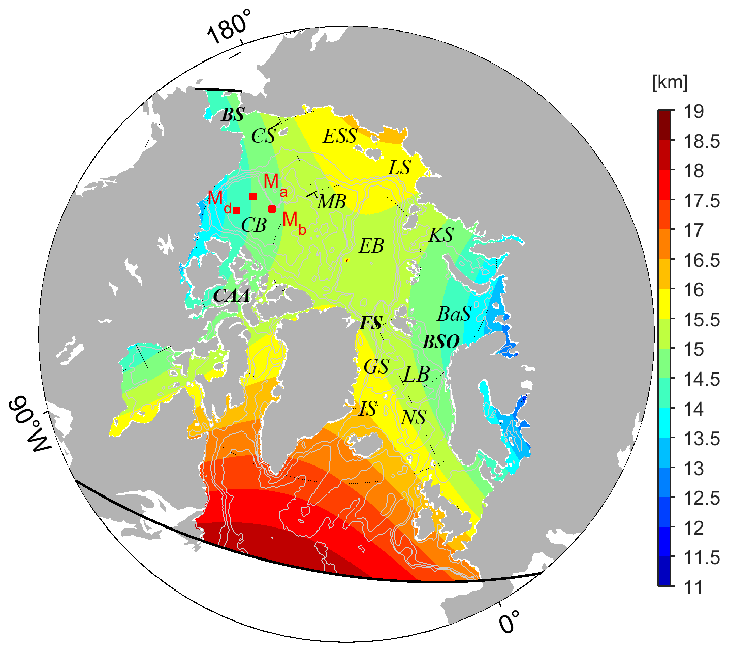
Figure 1 Map of the pan-Arctic regions showing the model domain (enclosed by the black lines) and horizontal resolutions (shading). The red rectangles show the three moorings (M_a, M_b, M_d) from the Beaufort Gyre Exploration Project (BGEP). Major basins and straits are labeled as follows: Canada Basin (CB), Makarov Basin (MB), Eurasian Basin (EB), Chukchi Sea (CS), East Siberian Sea (ESS), Laptev Sea (LS), Kara Sea (KS), Barents Sea (BaS), Greenland Sea (GS), Lofoten Basin (LB), Iceland Sea (IS), Norwegian Sea (NS), Bering Strait (BS), Fram Strait (FS), Barents Sea Opening (BSO), and Canadian Arctic Archipelago (CAA).

The adjoint method brings the model simulation close to available observations by iteratively adjusting control variables to minimize a quadric target function J (cost function hereinafter):

$$\begin{array}{}\text{(1)}& \begin{array}{rl}J\left({\mathbf{C}}_{\mathrm{ini}},{\mathbf{C}}_{\mathrm{atm}}\left(t\right)\right)& =\sum _{t=\mathrm{1}}^{T\mathrm{1}}{\left[\mathbf{y}\left(t\right)-\mathbf{E}\left(t\right)\mathbf{x}\left(t\right)\right]}^T\\ & \cdot {\mathbf{R}}^{-\mathrm{2}}\left[\mathbf{y}\left(t\right)-\mathbf{E}\left(t\right)\mathbf{x}\left(t\right)\right]\\ & +{\mathbf{C}}_{\mathrm{ini}}^T{\mathbf{P}}^{-\mathrm{2}}{\mathbf{C}}_{\mathrm{ini}}\\ & +\sum _{t=\mathrm{0}}^{T\mathrm{1}}{\mathbf{C}}_{\mathrm{atm}}{\left(t\right)}^T{\mathbf{Q}}_{\mathrm{a}}^{-\mathrm{2}}{\mathbf{C}}_{\mathrm{atm}}\left(t\right).\end{array}\end{array}$$

On the right-hand side of Eq. (1), the first term measures the model–data misfits weighted by the inverse error covariance matrices (R⁻²). The following section will introduce the available measurements and their uncertainties (R). The observations and model state at time t are denoted as y(t) and x(t), respectively; E(t) maps the model state x(t) to the corresponding observations y(t). The last two terms are background terms of the initial condition (C_ini) and the time-varying atmospheric forcing (C_atm(t)) weighted by their inverse error covariance matrices (P⁻² and ${\mathbf{Q}}_{\mathrm{a}}^{-\mathrm{2}}$, respectively), which penalize their adjustments and provide complete information on the controls. Following Lyu et al. (2021b), prior uncertainties of the time-varying atmospheric state (Q_a) depend on geographic locations. They are computed as the variance of the nonseasonal variability of the corresponding variables using NCEP-RA1.

For simplicity and the robust performance of this coupled data assimilation system, we choose the initial conditions (C_ini), including temperature, salinity, mean SIT, SIC, and daily atmospheric state on the model grid (C_atm(t)), which includes 10 m wind vectors, 2 m air temperature, 2 m specific humanity, precipitation, downwelling long-wave, and net short-wave radiation as the control variables. In the future development of ocean and sea ice state estimation systems, we further include the river runoff, open boundary conditions, and model parameter uncertainty as control variables as in previous studies (e.g., Fenty and Heimbach, 2013; Liu et al., 2012). In this study, we use a 1-year assimilation window covering the year 2012, resulting in a total number of $\sim \mathrm{2.7}\times {\mathrm{10}}^{\mathrm{8}}$ control variables.

During the optimization process, the adjoint of the coupled ocean and sea ice model is used to compute the gradients of the cost function J to the control variables, and a quasi-Newton algorithm (Gilbert and Lemaréchal, 1989) is used to iteratively reduce the cost function J. The optimization process continues until the cost function cannot be further reduced.

2.2 Observations and prior uncertainties

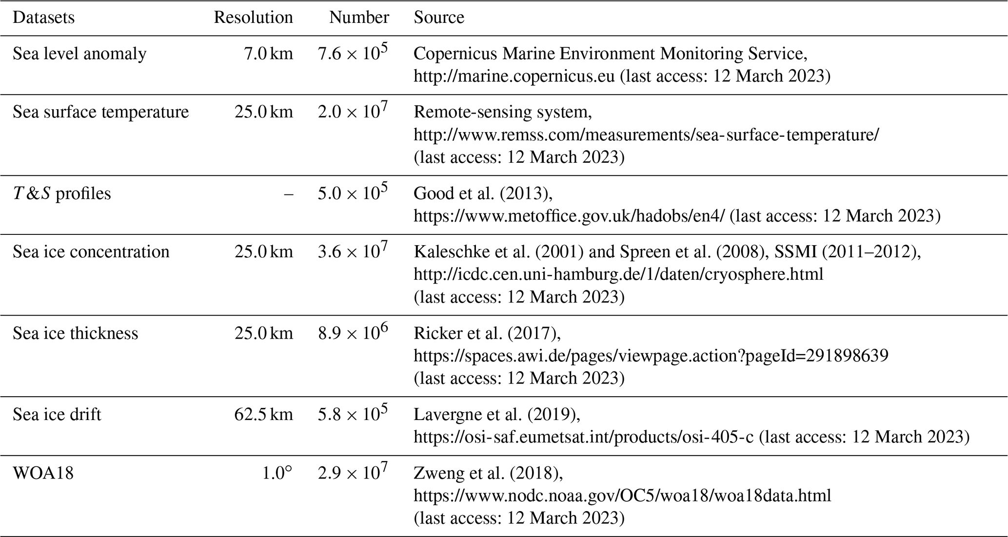
Both satellite and in situ measurements (Table 1) are used to constrain the model simulations. In addition, sea ice draft measurements by upward-looking sonar (ULS) from the Beaufort Gyre Exploration Project (BGEP, see Fig. 1 for the locations) are used to independently validate the assimilation results.

Prior uncertainties are detailed in our previous Arctic synthesis study (Lyu et al., 2021b). Uncertainties in temperature and salinity depend on the depth and are set to 0.6 ^∘C and 0.3 PSU at the surface and 0.02 ^∘C and 0.02 PSU in the deep ocean; SIC uncertainties consist of representation errors (15 % within 50 km from the coastlines and 10 % over the open water) and instrument errors. Because of higher errors in low SIC and lower errors over open water, we modify the representation uncertainties by multiplicative factors of 0.85, 1.20, 1.10, and 1.00 for the observed SIC ranges of 0.00, <15 %, 15 %–25 %, and >25 %, respectively.

The SIT errors are provided by the datasets and interpolated to our model grid. Sea level anomaly (SLA) uncertainties are set to 3.0 cm; SID uncertainties are dominated by representation errors and are set to 0.04 m s⁻¹. Sea surface temperature (SST) uncertainties are provided by the datasets. In addition, we reduce the weight of the temperature and salinity climatology (WOA18) cost components by factors of 20.0 and 10.0, respectively, to avoid overfitting to the climatology.

Table 1 Assimilated measurements.

2.3 Viscous-plastic sea ice dynamics and its adjoint

In the coupled ocean and sea ice model, the following equation governs sea ice drift:

$$\begin{array}{}\text{(2)}& m{\displaystyle \frac{\mathrm{d}\mathit{u}}{\mathrm{d}t}}=-mf\mathit{k}\times \mathit{u}+{\mathit{\tau }}_{\mathrm{air}}+{\mathit{\tau }}_{\mathrm{ocn}}-\mathrm{\nabla }\mathrm{\varnothing }\left(\mathrm{0}\right)+\mathrm{\nabla }\cdot \mathit{\sigma },\end{array}$$

where m is the sea ice mass and u is the sea ice motion vector; τ_air and τ_ocn are the wind and ocean drags, respectively; −∇∅(0) is the tilt of the sea surface; and ∇⋅σ is the divergence of the ice stress tensor σ_ij (i = 1, 2), representing the internal forces of sea ice.

In the viscous-plastic rheology of Hibler (1979), the stress tensor σ_ij is related to the sea ice strain rate (ϵ_ij) and strength (P):

$$\begin{array}{}\text{(3)}& \begin{array}{rl}{\mathit{\sigma }}_{ij}& =\mathrm{2}\mathit{\eta }\left({\mathit{ϵ}}_{ij},P\right){\mathit{ϵ}}_{ij}+\left[\mathit{\zeta }\left({\mathit{ϵ}}_{ij},P\right)-\mathit{\eta }\left({\mathit{ϵ}}_{ij},P\right)\right]{\mathit{ϵ}}_{kk}{\mathit{\delta }}_{ij}\\ & -{\displaystyle \frac{P}{\mathrm{2}}}{\mathit{\delta }}_{ij},\end{array}\end{array}$$

where δ_ij is the Kronecker delta (δ_ij=1 if i=j, otherwise 0); η and ζ are the bulk and shear viscosities, expressed as:

$$\begin{array}{}\text{(4)}& {\displaystyle }\mathit{\zeta }={\displaystyle \frac{P}{\mathrm{2}{\mathrm{\Delta }}_{\mathrm{reg}}}},\text{(5)}& {\displaystyle }\mathit{\eta }={\displaystyle \frac{P}{\mathrm{2}{e}^{\mathrm{2}}{\mathrm{\Delta }}_{\mathrm{reg}}}},\end{array}$$

where

$$\begin{array}{}\text{(6)}& \begin{array}{rl}\mathrm{\Delta }& =[\left({\mathit{ϵ}}_{\mathrm{11}}^{\mathrm{2}}+{\mathit{ϵ}}_{\mathrm{22}}^{\mathrm{2}}\right)\left(\mathrm{1}+e^{-\mathrm{2}}\right)+\mathrm{2}\left(\mathrm{1}-e^{-\mathrm{2}}\right){\mathit{ϵ}}_{\mathrm{11}}{\mathit{ϵ}}_{\mathrm{22}}\\ & +\mathrm{4}{e}^{-\mathrm{2}}{\mathit{ϵ}}_{\mathrm{12}}^{\mathrm{2}}{]}^{\frac{\mathrm{1}}{\mathrm{2}}},\end{array}\end{array}$$

where e is the ratio of normal stress to shear stress and is set to 2.0; ${\mathrm{\Delta }}_{\mathrm{reg}}=max(\mathrm{\Delta },{\mathrm{\Delta }}_{min})$ with Δ_min equals $\mathrm{1.0}\times {\mathrm{10}}^{-\mathrm{10}}$. The sea ice strain rate is computed as follows:

$$\begin{array}{}\text{(7)}& {\mathit{ϵ}}_{ij}={\displaystyle \frac{\mathrm{1}}{\mathrm{2}}}\left({\displaystyle \frac{\partial u_i}{\partial x_j}}+{\displaystyle \frac{\partial u_j}{\partial x_i}}\right).\end{array}$$

The sea ice strength P depends on mean SIT (H) and SIC (C):

$$\begin{array}{}\text{(8)}& P=P^{\ast }H\cdot \exp (-C^{\ast }\cdot (\mathrm{1}-C\left)\right),\end{array}$$

where P^* and C^* are the ice compressive strength constant and ice strength decay constant and are set to 2.75×10⁴ N m⁻² and 20.0, respectively.

The dependence of the internal force term (∇⋅σ) on ice velocity is strongly nonlinear, leading to an unstable adjoint of the coupled ocean and sea ice system. Therefore, previous studies (Koldunov et al., 2017; Lyu et al., 2021b) used an adjoint of a free-drift sea ice model (without an adjoint of ∇⋅σ). Toyoda et al. (2019) pointed out that the full adjoint of Eq. (2) can be stabilized by eliminating the dependence of bulk and shear viscosities on the strain rate (ϵ_ij).

Following the study of Toyoda et al. (2019), we eliminate the dependence of bulk and shear viscosities on ϵ_ij in the adjoint of Eq. (2). In addition, we note that there are still strong sensitivities that hamper the convergence of optimization. We set the adjoint sensitivities of ice velocity to zero if the local sensitivity is 50 times larger than the global mean of their absolute values. In addition, we also modify the adjoint model in the following ways to ensure the stability of the adjoint model over a 1-year assimilation window:

1. Disable the K-Profile parameterization mixing.

2. Increase the Laplacian horizontal diffusivity of heat and salinity to 500 m² s⁻¹ and lateral eddy viscosity to 10 000 m² s⁻¹.

3. Apply a spatial filter to sensitivity variables calculated in the adjoint of the thermodynamic sea ice model (see Appendix in Lyu et al., 2021b, for details).

Since the sea ice dynamic model is solved using an iterative line successive over-relaxation solver, we note that the approximated adjoint of the viscous-plastic sea ice dynamics (adjoint-VP) requires ∼ 1.2 times the computational cost of using the adjoint of a free-drift sea ice model (adjoint-FD).

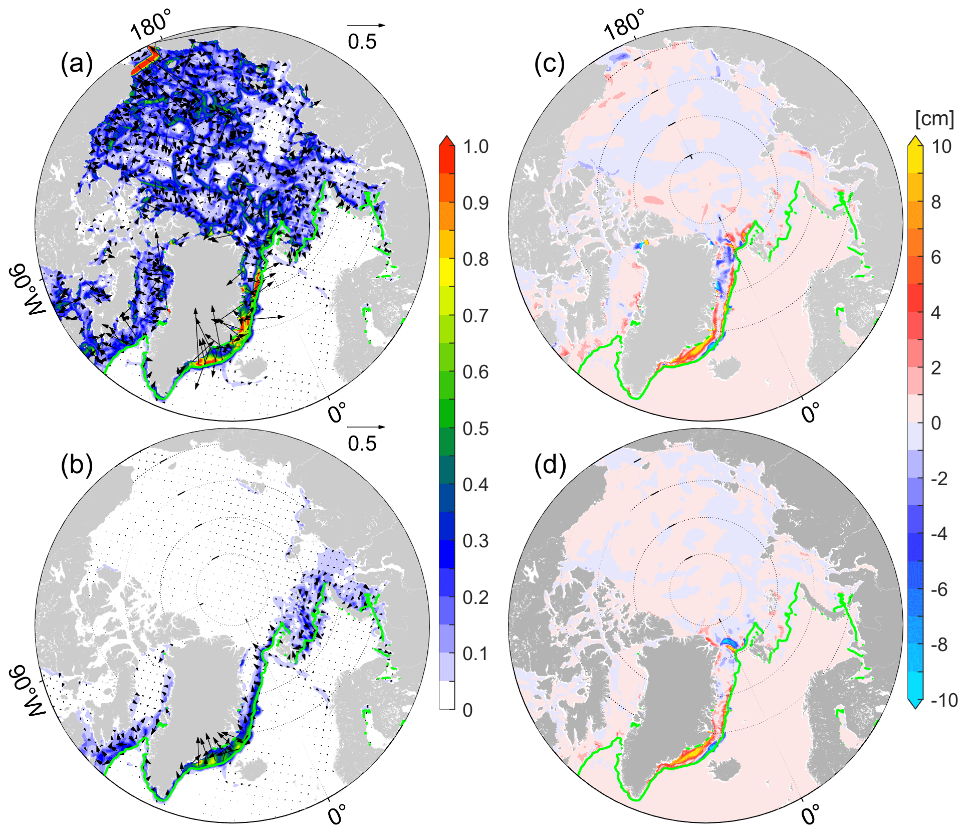
Figure 2 Sensitivities of total sea ice volume to wind vectors (in 0.1× km³ (m s⁻¹)⁻¹, shadings represents amplitudes) using the adjoint of (a) free-drift sea ice dynamics and (b) viscous-plastic sea ice dynamics with modifications in Sect. 2.3. Panels (c)–(d) show the mean SIT changes by perturbing the wind with the corresponding adjoint sensitivities multiplied by a factor of 10⁻⁸. The green lines are the sea ice extents (SIEs, 15 % SIC) in January 2012.

Based on adjoint-FD and adjoint-VP, we compute the sensitivities of domain-integrated sea ice volume (SIV) with respect to the atmospheric forcings and the initial conditions over the period from 1 to 31 January 2012. As reported by Toyoda et al. (2019), adjoint-FD shows much stronger sensitivities to wind than adjoint-VP does (Fig. 2a, b) in the central Arctic Ocean. Along the sea ice marginals (SIMs) of the Atlantic sectors, adjoint-VP reveals that the towards-ice wind anomalies increase total sea ice (Fig. 2b) since they prevent ice from drifting to the warm Atlantic water. However, adjoint-FD shows strong sensitivities along the SIMs of the Atlantic sectors, but both towards-ice and off-ice wind anomalies appear (Fig. 2a), potentially resulting in ice convergence.

Furthermore, we add daily wind perturbations, computed by scaling the adjoint sensitivities (Fig. 2a, b) so that the maximum perturbations are 1.0 m s⁻¹ to the 6-hourly wind from NCEP-RA1 and examine their impacts on mean SIT changes. As expected, mean SIT changes are mainly along the SIMs in the Atlantic sectors (Fig. 2c, d), and wind perturbations from adjoint-FD reduces mean SIT northeast of Greenland (Fig. 2c). In the central Arctic Ocean with compact ice, the internal forces ∇⋅σ oppose the impacts of wind perturbations. Therefore, despite the strong adjoint sensitivities to the wind in adjoint-FD, we note that the resulting wind perturbations only slightly change the mean SIT (Fig. 2c), which is comparable to that in adjoint-VP (Fig. 2d).

In addition to overestimating the sensitivities to wind, adjoint-FD may degrade the usefulness of the adjoint sensitivities in optimization. Therefore, we perform two assimilation experiments to comprehensively evaluate the impacts of including the approximate adjoint of sea ice rheology on ocean and sea ice estimations.

3 Model–data misfit reductions and residuals

3.1 Evaluation of the optimization

In this study, we consider iteration 0 to be the control run. In adjoint-FD and adjoint-VP, the optimizations stall at iterations 13 and 32, and the further cost-function reductions at the last two successive iterations are 0.7 % and 0.2 % of the total cost, respectively. After the optimizations, the total cost and norms of the gradients are reduced by 32.3 % and 59.2 %, respectively, in adjoint-FD and by 40.2 % and 89.3 %, respectively, in adjoint-VP.

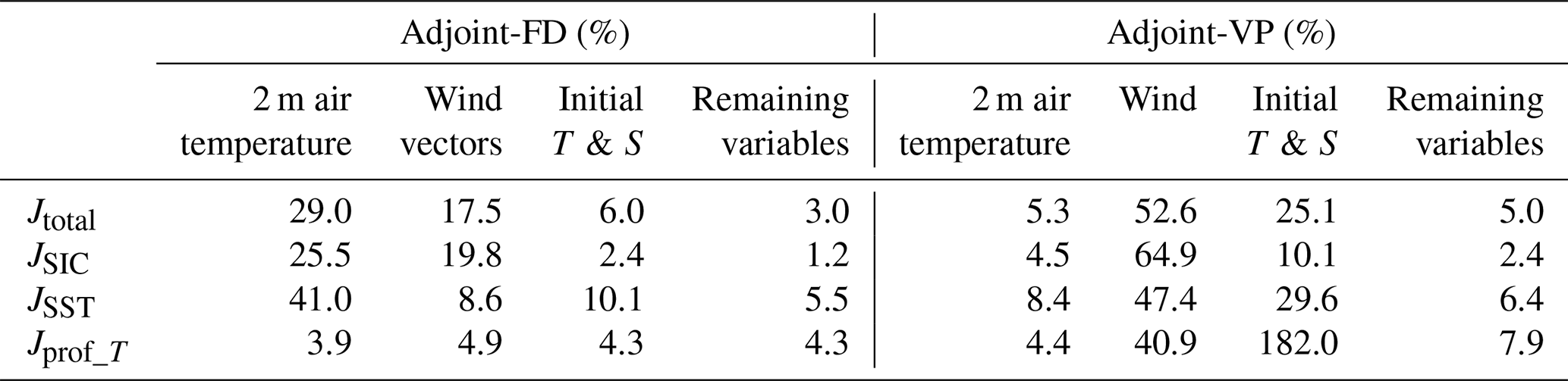
Table 2 Normalized costs and reductions in the two optimization runs.

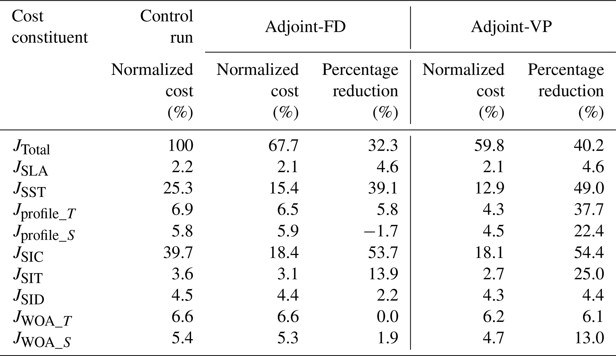
Of the individual cost constituents (Table 2), satellite-observed SST (J_SST) and SIC (J_SIC) contribute ∼ 25.3 % and 39.7 % of the total cost, respectively, which are significantly reduced after optimization. The costs of the temperature (J_{profile_T}) and salinity (J_{profile_S}) profiles are also considerably reduced, especially in the adjoint-VP. The rest of the cost constituents are also slightly reduced. Overall, including the adjoint of sea ice rheology further reduces the total cost by 7.9 % and the individual cost constituents, especially J_SST, J_{profile_T}, and J_{profile_S}. Based on iterations 0 and 13 in adjoint-FD, and 32 in adjoint-VP of the optimization, we will focus on the sea ice state and ocean temperature to evaluate the impacts of using this approximate adjoint of sea ice rheology.

3.2 Sea ice state

3.2.1 Residual errors of SIC and SIT

Satellite visible, infrared, and microwave technologies have been applied to monitor SIC with high frequencies and quality, which is of high priority in global and Arctic-focused synthesis (Chevallier et al., 2017; Uotila et al., 2019). Previous studies (Fenty and Heimbach, 2013; Lyu et al., 2021a, b) indicated that SIC could be significantly improved by slightly adjusting the atmospheric forcings. Here, we explore the residual errors in the optimization runs.

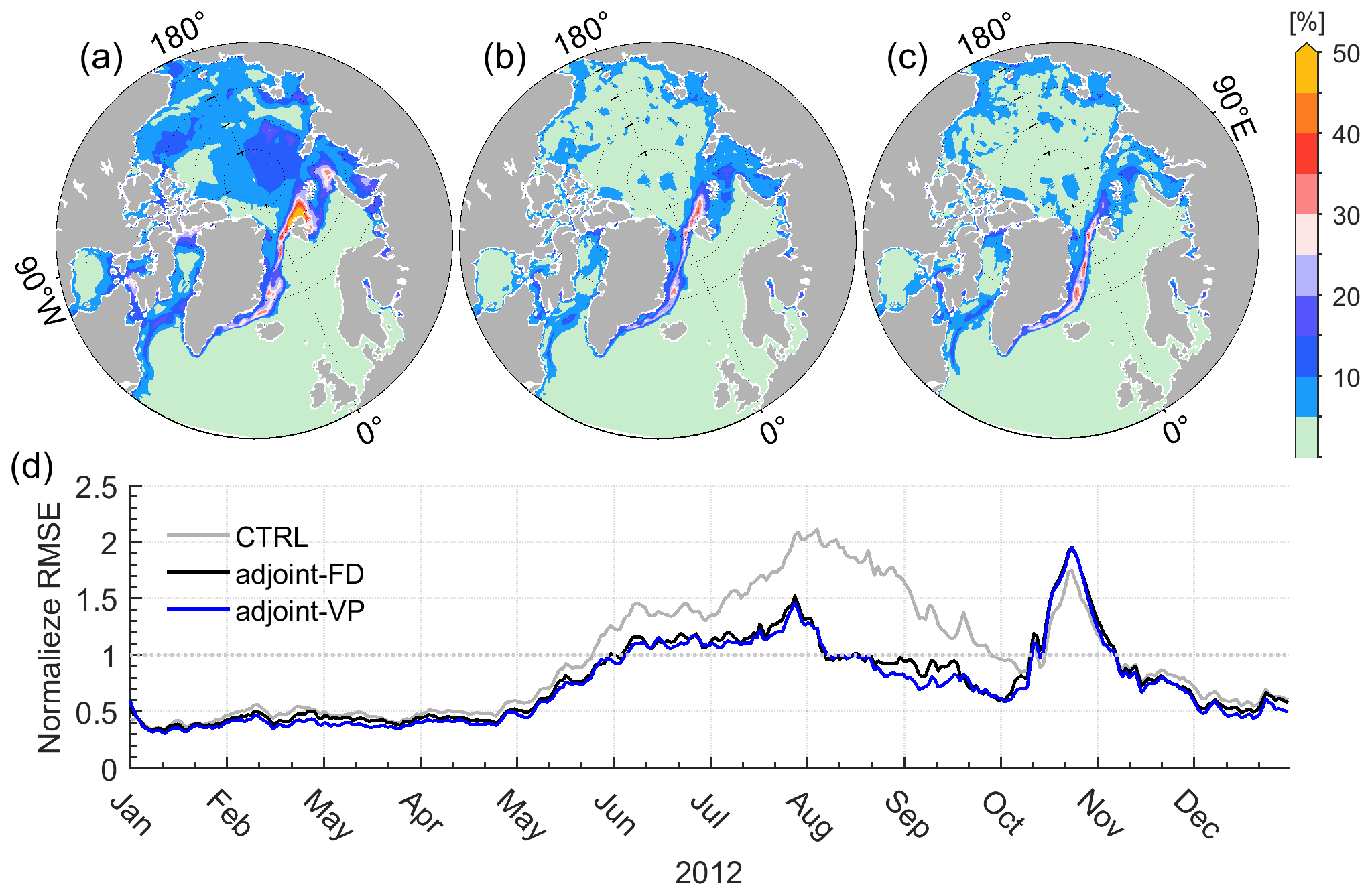
Figure 3 Root mean square errors (RMSEs) of SIC between the satellite measurements and (a) the control run, (b) adjoint-FD, and (c) adjoint-VP averaged over 2012. Panel (d) shows the temporal variations in RMSEs normalized by prior uncertainties in the three simulations averaged over the regions covered by sea ice.

The root mean square errors (RMSEs) of SIC averaged over 2012 (Fig. 3a–c) and normalized by the prior errors and averaged over the model domain (Fig. 3d) show the geographical distribution and temporal evolution of SIC errors, respectively. The normalized RMSEs in Fig. 3d should be close to 1.0 if the optimization found a model simulation consistent with the observations and the prior uncertainties.

The control run (Fig. 3a) shows pronounced RMSEs in the Beaufort Gyre (∼ 15 %), the central Eurasian Basin (15 %–20 %), the marginal seas (15 %–20 %), and SIMs of the Atlantic sector (30 %–50 %). The normalized RMSEs reveal that SIC errors remain small (∼ 0.5) in the wintertime (Fig. 3d), indicating that the control run and the satellite SIC measurements match well, but they grow quickly from May to September when the sea ice melts (Fig. 3d). Normalized RMSEs up to 1.5 are observed in October but quickly drop in November (Fig. 3d). Therefore, SIC errors are significant during the melting and refreezing periods (from May to November).

Both assimilation experiments reduce the SIC errors to less than 5 % in the central Arctic Ocean and 10 % in the marginal seas. SIC errors of up to 20 % persist in the Atlantic sector, where sea ice shows strong nonlinearity and the tangent linear model can capture only part of the sea ice changes (Appendix B in Lyu et al., 2021a). Normalized SIC errors from May to September are also reduced to nearly 1.0 by assimilation of the daily SIC observations (Fig. 3d). However, SIC errors in October remain significant (Fig. 3d) since the observed sea ice recovers much faster than in the control run and the two assimilation runs (not shown here). This delayed sea ice recovery in the model may be related to model parameter uncertainties, such as the threshold thickness between thin and thick ice, which determines the initial sea ice thickness formed in open water.

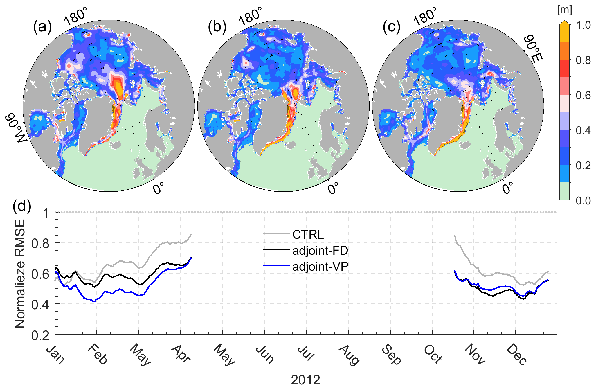
Figure 4 Root mean square errors (RMSEs) of SIT between the satellite measurements and (a) the control run, (b) adjoint-FD, and (c) adjoint-VP averaged over 2012. Panel (d) shows the temporal variations in RMSEs normalized by prior uncertainties in the three simulations averaged over the regions covered by sea ice.

The control run shows SIT errors of up to 1.0 m in regions north and south of the Fram Strait and approximately 0.4–0.7 m in the Beaufort Gyre. In the Beaufort Gyre, the SIT errors are reduced to less than 0.3 m in adjoint-VP (Fig. 4c) and approximately 0.3–0.5 m in adjoint-FD (Fig. 4b). Similar to the SIC errors, SIT errors of up to 1.0 m remain along the East Greenland Current, which seems to increase in the two assimilation experiments. The temporal evolutions of normalized RMSEs show that the SIT errors grow quickly from February to April (Fig. 4d). Both assimilation experiments reduce the SIT errors, especially in adjoint-VP from January to April (Fig. 4d). However, the normalized RMSEs of SIT averaged over the model domain remain smaller than 1.0 and seem to grow during the melting season. Again, the normalized SIT errors of smaller than 1.0 indicates that SIT uncertainties are too large, and more accurate SIT observations (e.g., half of the uncertainties) and SIT observations during the melting season are required to facilitate a significant impact on the model simulation.

3.2.2 BGEP mooring measurements

Independent sea ice draft measured by upward-looking sonar (ULS) on the BGEP moorings (M_a, M_b, and M_d in Fig. 1) is used to validate the simulated sea ice draft. The simulated snow depth (d_snow) and SIT (d_SIT) are used to compute the sea ice draft following the methods of Tilling et al. (2018):

$$\begin{array}{}\text{(9)}& \mathrm{draft}={\displaystyle \frac{{\mathit{\rho }}_{\mathrm{i}}\times d_{\mathrm{SIT}}+{\mathit{\rho }}_{\mathrm{s}}\times d_{\mathrm{snow}}}{{\mathit{\rho }}_{\mathrm{w}}}},\end{array}$$

where ρ_i, ρ_s, and ρ_w are the densities of the sea ice, snow, and water, respectively, and are set to 910.0, 330.0, and 1027.5 kg m⁻³, respectively, as in our model.

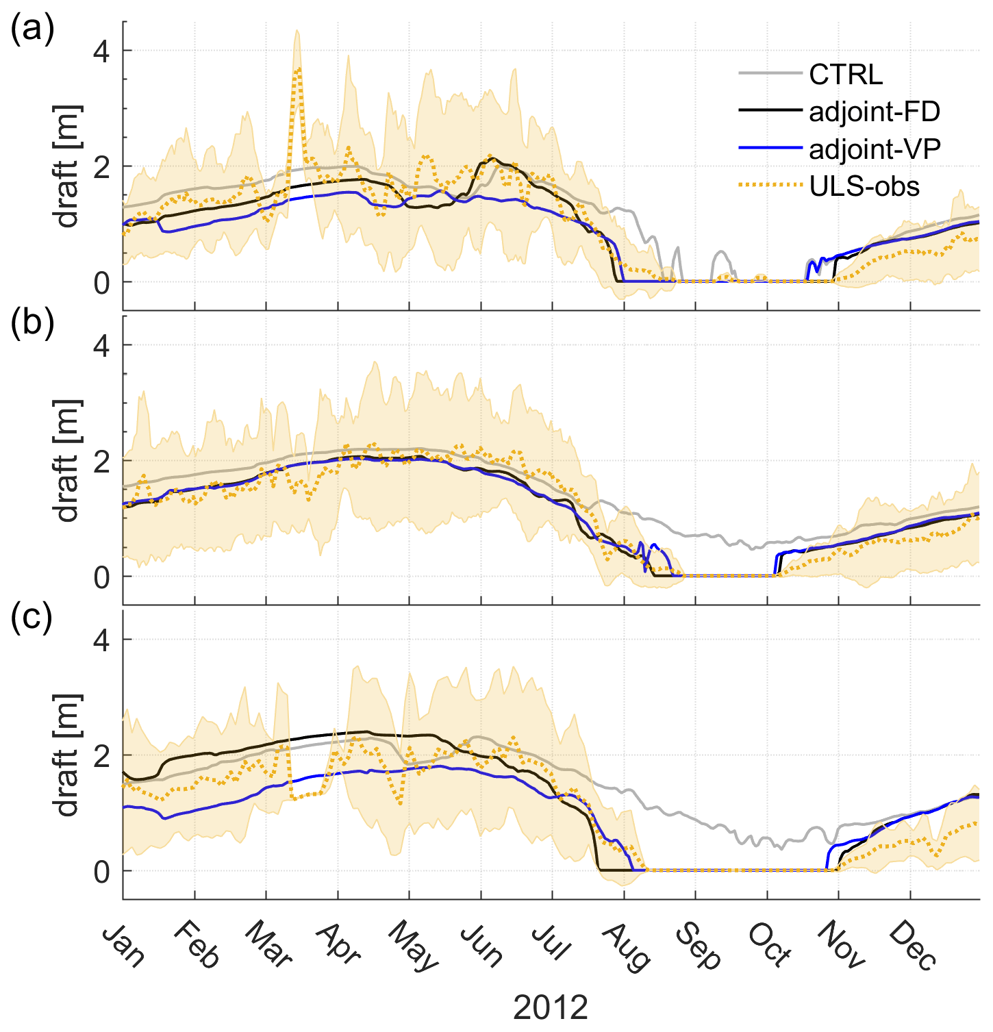
Figure 5 Daily time series of the sea ice draft (dotted yellow lines) and the daily standard deviation (shadings) at the mooring locations (a) M_a, (b) M_b, and (c) M_d compared to the control run and the two assimilation runs (see the legend) throughout the year 2012. ULS-observed sea ice drafts are smoothed with a 5 d running average.

The ULS measurements depict stronger daily to sub-monthly sea ice draft variability than the model simulations do, which may be related to ice flow motions. The control run simulates a delayed ice disappearance process in M_a (Fig. 5a) and fails to reproduce the sea ice disappearance processes in M_b (Fig. 5b) and M_d (Fig. 5c) from August to October. After optimization, adjoint-VP and adjoint-FD reproduce the sea ice melting and refreezing processes well, although errors of up to 0.5 m remain from January to June. Overall, the two assimilation runs reproduce the local sea ice retreat and recovery process well.

3.3 Ocean temperature

Ocean temperature changes are closely related to sea ice changes. Adjoint-VP introduces more pronounced ocean temperature changes than adjoint-FD does. Here, we explore ocean temperature changes after assimilation.

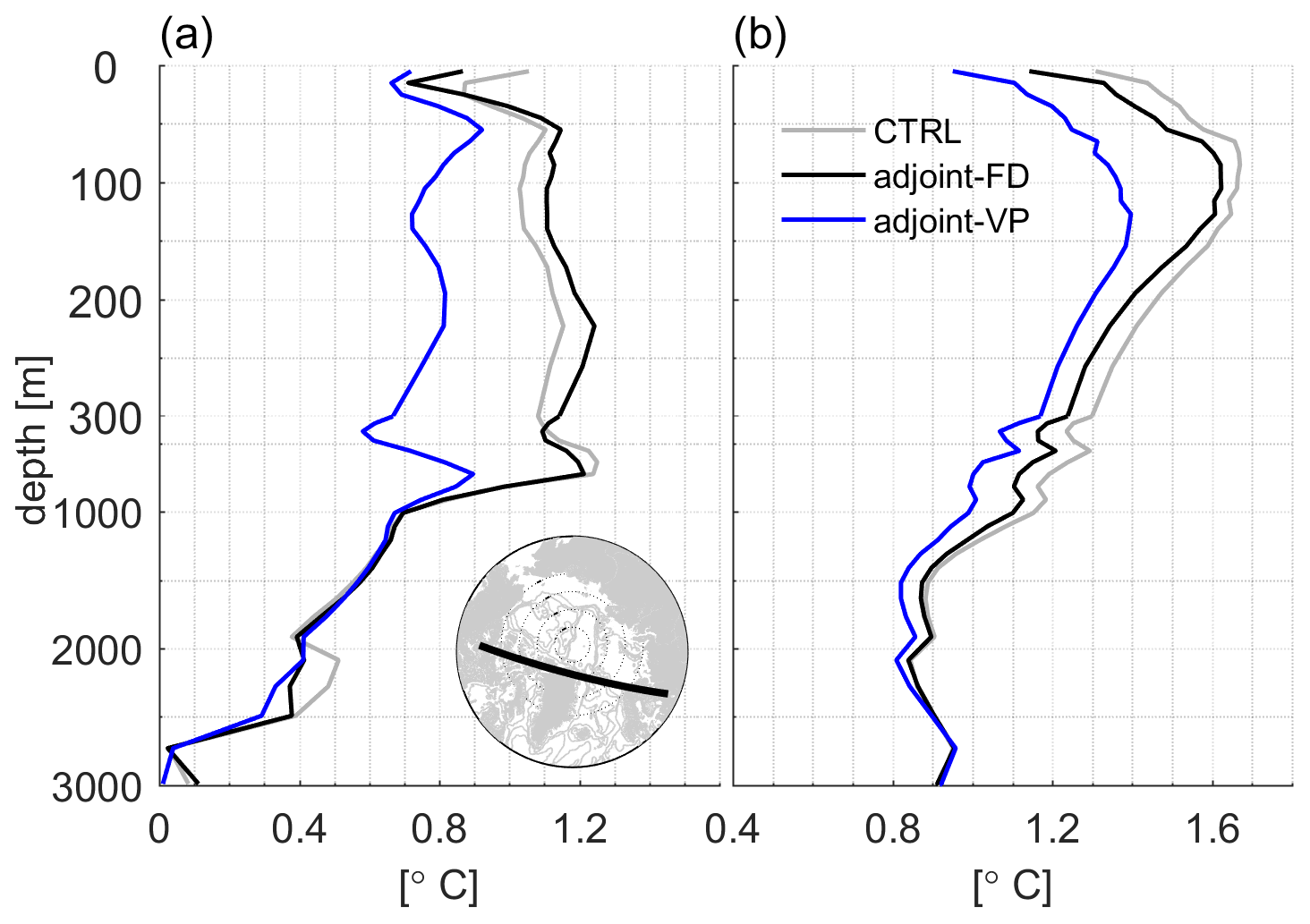
Figure 6 RMSEs of potential temperature in the (a) Arctic Ocean and (b) North Atlantic Ocean in the three runs. The Arctic Ocean and the North Atlantic Ocean are separated by the black lines in the bottom subplot.

In the Arctic Ocean, adjoint-FD reduces temperature errors only over the top 20 m, while adjoint-VP reduces temperature errors up to 0.4 ^∘C over the top 1000 m (Fig. 6a). In the North Atlantic Ocean, adjoint-VP results a in more pronounced RMSE reduction up to 0.3 ^∘C more than adjoint-FD (Fig. 6b).

Relative temperature error reductions over the top 50 m reveal an overall improvement in temperature with occasional degradation (Fig. 7a, b). Adjoint-VP results in a more significant error reduction than does adjoint-FD in the North Atlantic Ocean (Fig. 7a, b). In the southern Beaufort Gyre, the Laptev and Kara seas, and north of Svalbard, both adjoint-VP and adjoint-FD increase the ocean temperature (over 50 m) since the two optimization runs reproduce the early retreat of the sea ice well, allowing more solar heating of the open water. In the North Atlantic Ocean, adjoint-VP achieves more considerable temperature changes than does adjoint-FD, both over the top 50 m (Fig. 7c, d) and from 50 to 700 m (Fig. 7e, f). In the Arctic Ocean, adjoint-VP further introduces negative temperature corrections between 50 and 700 m (Fig. 7f), especially near the profile locations (see dots in Fig. 7b).

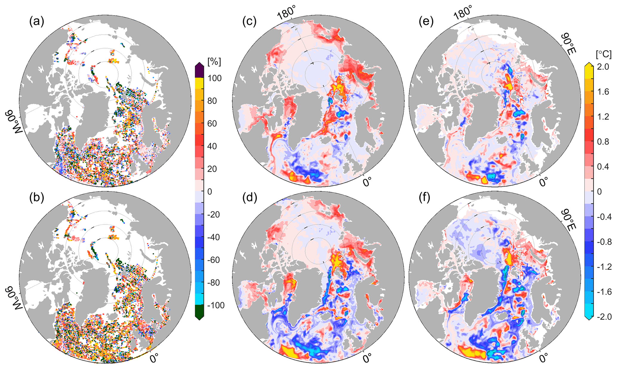
Figure 7 Relative temperature error reduction ($-\frac{\left|T_{\mathrm{opti}}-T_{\mathrm{obs}}\right|-\left|T_{\mathrm{ctrl}}-T_{\mathrm{obs}}\right|}{\left|T_{\mathrm{ctrl}}-T_{\mathrm{obs}}\right|}\times \mathrm{100}$ %) over the top 50 m at the profile locations in (a) adjoint-FD and (b) adjoint-VP. Values >100 % indicate overadjustment. Panels (c) and (d) show the temperature differences of adjoint-FD and adjoint-VP to the control run averaged over the top 50 m, respectively. Panels (e) and (f) are the same as (c) and (d), but for the 50–700 m layers.

In summary, adjoint-FD and adjoint-VP reproduce the SIC variations well in the Arctic Ocean, which further reduces ocean temperature errors in the top layer by improving the atmosphere–ocean heat flux. Adjoint-VP achieves more significant corrections to the ocean temperature over the open water and in the intermediate layer of the Arctic Ocean than adjoint-FD does.

4 Adjustment of the control variables

The adjoint models project the model–data misfits onto the gradient of the cost function with respect to all control variables simultaneously, which is used by the optimization algorithm to adjust the control variables. In this section, we compare adjustments of the control variables in the adjoint-FD and adjoint-VP and evaluate contributions of individual adjustments of the control variables on the cost-function reduction. We also compare the adjustments of the control variables in adjoint-FD and adjoint-VP with differences between ERA5 (Hersbach et al., 2020) and NCEP-RA1 reanalyses.

Among all the control variables, wind vectors and 2 m air temperature are considerably adjusted in adjoint-FD and adjoint-VP but also show significant differences. In addition, adjoint-VP induces more pronounced adjustments of the initial temperature and salinity than adjoint-FD does (not shown here). Here, we concentrate on the adjustments of wind vectors and the 2 m air temperature.

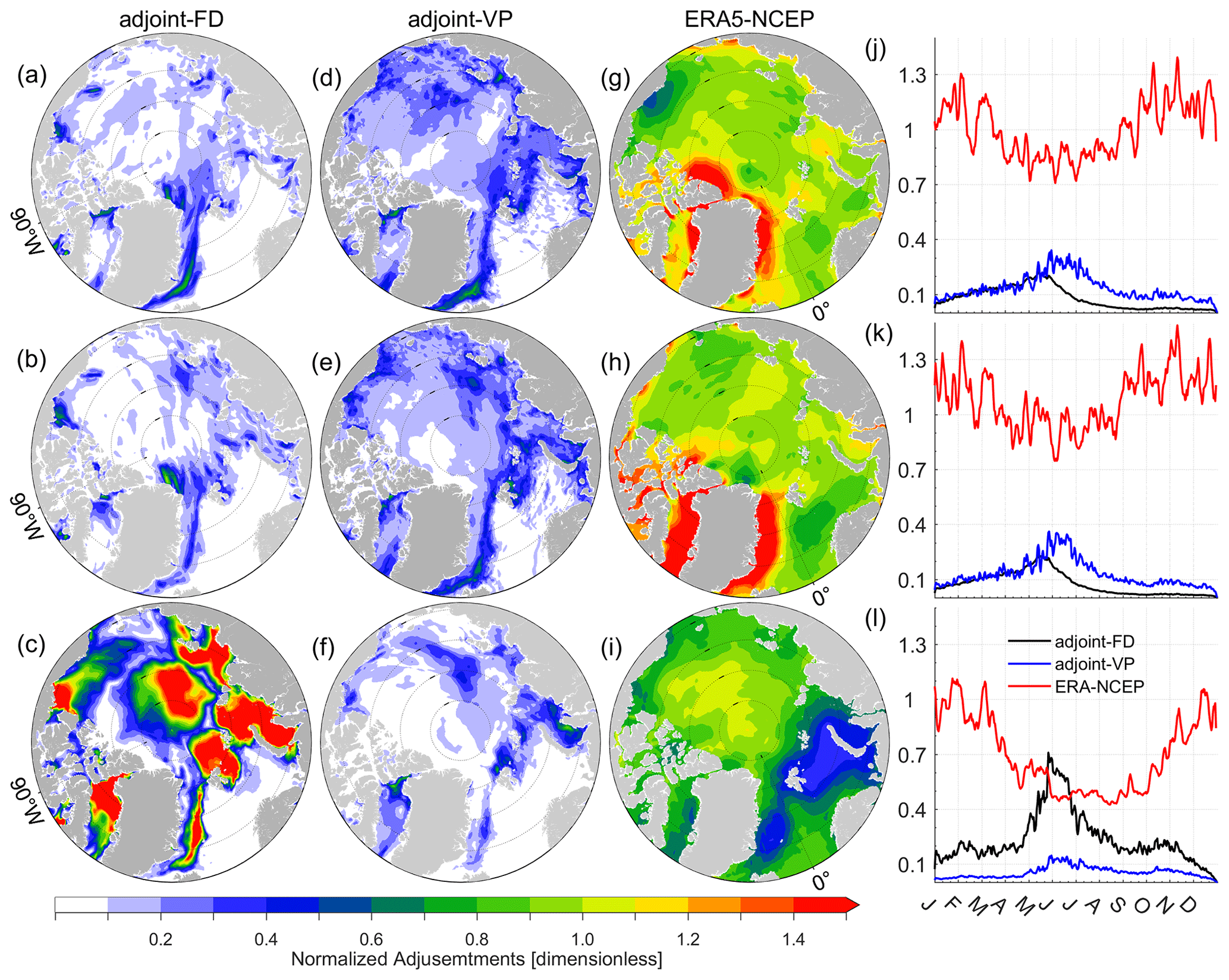
Figure 8 Root mean square (RMS) of the adjustments of the (a) wind u component, (b) wind v component, and (c) 2 m air temperature normalized by their prior uncertainties (dimensionless) in adjoint-FD and averaged over 2012. Panels (d)–(f) are similar to (a)–(c) but for adjoint-VP. Panels (g)–(i) show the normalized RMS of differences in the (g) wind u component, (h) wind v component, and (i) 2 m air temperature between ERA5 and NCEP-RA1 reanalyses (normalized by prior uncertainties in assimilation experiments). Panels (j)–(l) are the area averages of the normalized RMS of adjustments (differences) of the wind u component, wind v component, and 2 m air temperature (dimensionless) in adjoint-FD and adjoint-VP (ERA5-NCEP).

Figure 8 shows the root mean square (RMS) of the adjustments of the wind vectors and 2 m air temperature normalized by their prior uncertainties. The normalized RMS of the adjustments of the control variables should be smaller than 1.0 if the adjustments are within their prior uncertainties. Adjoint-FD slightly adjusts the wind vectors (with the normalized RMS of the adjustments being smaller than 0.4, Fig. 8a, b), but the 2 m air temperature is significantly adjusted (with the normalized RMS of adjustments being greater than 1.5, Fig. 8c). In adjoint-VP, the wind vectors and 2 m air temperature are slightly adjusted (Fig. 8d–f) with their normalized RMS of adjustments being smaller than 0.3. In addition to the different amplitudes of the adjustments, the maximum adjustments of the wind vectors appear in June in adjoint-VP but in May in adjoint-FD (Fig. 8j, k). Throughout 2012, the 2 m air temperature is adjusted more prominently in adjoint-FD than in adjoint-VP (Fig. 8l).

We note that the adjustments of the three atmospheric state variables in Fig. 8a–f resemble the SIC (Fig. 3a) and SIT (Fig. 4a) error patterns, indicating that these adjustments are mostly determined by sea ice state errors that are projected on the control variables by the adjoint models rather than the background terms (the second and third terms on the right-hand side of Eq. 1). Excluding the adjoint of sea ice rheology (adjoint-FD) results in overadjustments of 2 m air temperature. With an approximated adjoint of sea ice rheology (adjoint-VP), we reduce the model–data misfits by slightly adjusting the control variables. The normalized adjustments of 0.1–0.6 indicate that the estimated prior uncertainties of the atmospheric state remain too large.

Using the new generation ERA5 reanalysis, we further compare the ERA5-NCEP differences against the adjustments of the atmosphere state variables in terms of their spatial patterns and temporal variability. The ERA5 uses fractional SIC as surface boundary conditions, but NCEP-RA1 uses 0 and 1 for ice-free and ice-covered ocean, respectively. The purpose of this comparison is twofold: (1) it further justifies the rationale of the adjustment amplitudes and (2) it examines whether the adjustments reflect the differences between the old generation NCEP-RA1 reanalysis and the new generation ERA5 reanalysis. For the wind vectors, the normalized RMS differences between the ERA5 and NCEP-RA1 reanalyses (Fig. 8g, h) are much larger than the wind vector adjustments in adjoint-FD (Fig. 8a, b) and adjoint-VP (Fig. 8d, e). For the 2 m air temperature, the normalized ERA5-NCEP differences (>1.0, Fig. 8i) are much larger than the normalized adjustments in adjoint-VP (<0.3, Fig. 8f) but smaller than the normalized adjustments in adjoint-FD (>1.5, Fig. 8c) in the Kara Sea, the Laptev Sea, the southern Beaufort Sea, the Eurasian Basin, and the Makarov Basin. It is evident that the 2 m air temperature adjustments in adjoint-FD are too large. Averaged over the model domain and throughout 2012, the ERA5-NCEP differences are much larger than the adjustments (Fig. 8j–l) in the two assimilation runs. In addition, the adjustments are larger from May to August than from September to April, while the ERA5-NCEP differences are larger in the winter season than in the summer season (Fig. 8j–l). The comparisons confirm that the 2 m air temperature is overadjusted in adjoint-FD, especially from May to July (Fig. 8l). The adjustments of wind vectors and 2 m air temperature do not resemble the ERA5-NCEP differences, indicating that the model–data differences cannot be fully fixed by replacing the old generation NCEP-RA1 reanalysis with the new generation ERA5 reanalysis.

Table 3 Contributions of the adjustments of 2 m air temperature, wind vectors, initial temperature and salinity (initial T & S), and the remaining control variables (including initial mean SIT and SIC, 2 m specific humanity, precipitation, downwelling longwave, and net short-wave radiation) on the total cost reduction, SIC, SST, and temperature profiles in the two optimization runs.

By replacing the adjusted initial temperature and salinity, wind vectors, 2 m air temperature, and the remaining control variables with NCEP-RA1 datasets, we integrate the model and estimate the contributions of these variables to the total cost reductions and individual components. Table 3 summarizes the contribution of individual control variables to the total cost reductions and cost components of SIC, SST, and temperature profiles.

The small contributions of the adjustments of the remaining control variables (“Remaining variables” in Table 3) to the cost-function reductions in adjoint-FD and adjoint-VP highlight the importance of simultaneous adjustments of the initial temperature and salinity, wind vectors, and 2 m air temperature. In adjoint-FD, the adjustments of the 2 m air temperature and wind vectors dominate the cost-function reduction, especially the SIC components. In contrast, adjoint-VP relies more on the adjustments of the wind vectors and the initial temperature and salinity. Besides, the more pronounced ocean temperature improvements (see Fig. 7) in adjoint-VP are mostly attributed to the adjustments in the initial temperature and salinity (Table 3).

Overall, adjoint-FD attributes more of the model–data misfits to the 2 m air temperature than the adjoint-VP does, resulting in overadjustments of the 2 m air temperature. By using an approximated adjoint of the sea ice rheology (adjoint-VP), we reduce the model–data misfit by slightly adjusting the control variables. This leads to the conclusion that the large 2 m air temperature adjustments in adjoint-FD is likely an overcompensation for wind errors that cannot be appropriately corrected because of large errors in the respective cost-function gradients.

5 The impacts on sea ice retreat processes

A unique characteristic of the adjoint-based reanalysis is that its physical processes are described by the governing equations of the model, allowing us to quantify the sea ice loss and the contributions of the sea ice dynamics and sea ice–ocean–atmosphere fluxes through a closed budget analysis. In this section, we explore and compare the mean SIT changes based on the model-governing equation:

$$\begin{array}{}\text{(10)}& {\displaystyle \frac{\mathrm{d}h}{\mathrm{d}t}}=-\mathrm{\nabla }\cdot \left(\mathit{u}h\right)+F_{\mathrm{oi}}+F_{\mathrm{ai}}+F_{\mathrm{res}}.\end{array}$$

The mean SIT tendency $\frac{\mathrm{d}h}{\mathrm{d}t}$ is dominated by the sea ice advective flux ($-\mathrm{\nabla }\cdot \left(\mathit{u}h\right)$), ocean–sea ice heat flux (F_oi) at the sea ice bottom, atmosphere–sea ice flux (F_ai) at the sea ice surface, and a residual term (F_res) including a snow-flooding effect and a source term to correct negative mean SIT to zero. The F_oi depends on the ocean temperature difference from freezing temperature (Maykut and McPhee, 1995) and F_ai consists of the radiation and turbulence fluxes over the sea ice surface. The contributions of the residual terms are small and therefore we do not show them in the analysis below.

By integrating the mean SIT over the Arctic Ocean (see Fig. 9 for the locations), we derive Arctic sea ice volume (SIV) changes. As shown in Fig. 9a, the two assimilation runs change the total Arctic SIV changes in different ways. Adjoint-VP reduces the Arctic SIV by reducing the initial Arctic SIV and changing the SIV tendency from May to August. By September, adjoint-VP simulates more sea ice than the control run. Adjoint-FD slightly increases the initial SIV, and the signals are invisible by February 2012. From May to July, adjoint-FD shows a stronger sea ice melting process than the control run and adjoint-VP. By September, adjoint-FD simulates the most SIV among the three simulations.

Based on Eq. (10), we further compare SIV tendencies and the budget terms in the two assimilation runs (Fig. 9b). The two assimilation runs reveal that the seasonal SIV changes are dominated by F_ai (magenta lines in Fig. 9b). Throughout the year, the ocean melts the sea ice from the bottom (blue lines in Fig. 9b) and net sea ice transport also reduces the Arctic sea ice (green lines in Fig. 9b). However, we note that a much stronger sea ice loss process occurs from 20 May to 15 June in adjoint-FD (up to −193.0 km³ d⁻¹) than in adjoint-VP (up to −125.0 km³ d⁻¹), which is mainly attributed to F_ai anomalies (magenta lines in Fig. 9b).

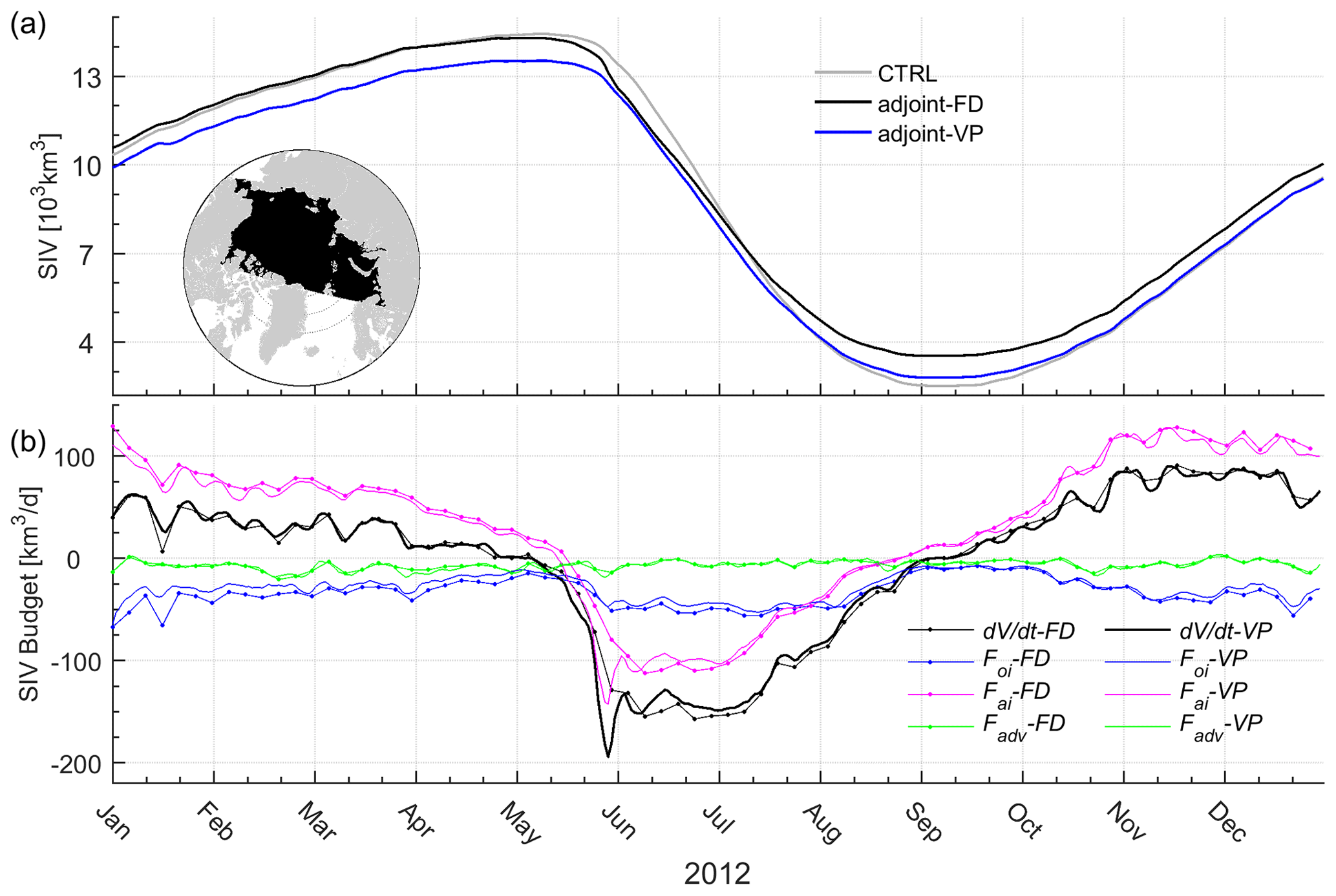
Figure 9 (a) SIV changes in the Arctic Ocean (see the bottom left subplot in a) from January to December 2012. (b) SIV tendencies and contributions from F_oi, F_ai, and F_adv in adjoint-FD and adjoint-VP (see the legend).

From 20 May to 15 June, the Arctic Ocean observations mostly rely on satellite-measured SIC. Both the two optimization runs reproduce the observed sea ice extents (SIEs, 15 % SIC) well on 15 June (green and red lines in Fig. 10a, d), with adjoint-VP slightly better than adjoint-FD in the Barents and Kara seas (Fig. 10a, d).

On 20 May, adjoint-FD simulates more sea ice than adjoint-VP does (Fig. 9a). From 20 May to 15 June, adjoint-FD destroys the extra sea ice in the southeastern Beaufort Gyre, the Laptev Sea, the Kara Sea, and north of Svalbard and Franz Josef Land through a stronger surface melting F_ai (Fig. 10b). At the same time, F_ai results in less sea ice loss (up to 0.6 m) in adjoint-FD in the central Arctic Ocean. Near the SIMs, F_adv differences determine the mean SIT differences (Fig. 10a, c). In contrast, mean SIT differences from 20 May to 15 June between adjoint-VP and the control run (Fig. 10d) are mostly caused by F_adv differences (Fig. 10f) and F_ai differences have little contribution (Fig. 10e), indicating that adjoint-VP modifies the SID to improve the model simulation during this period.

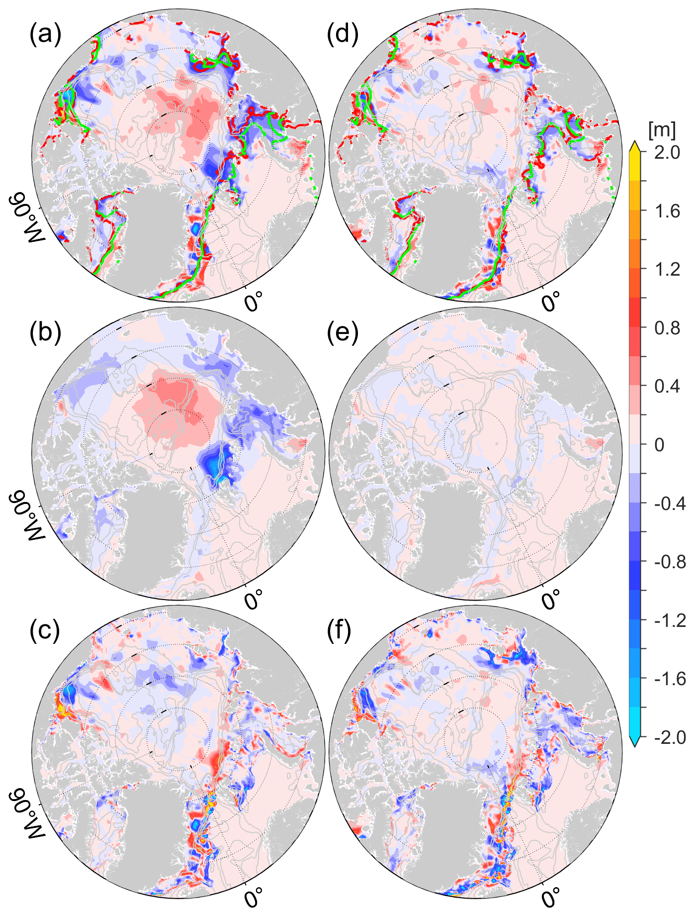
Figure 10 (a) Differences in $\int \frac{\mathrm{d}h}{\mathrm{d}t}$ integrated from 20 May to 15 June between adjoint-FD and the control run (adjoint-FD minus the control run), attributed to (b) ∫F_ai and (c) ∫F_adv differences. Panels (c)–(f) are the same as (a)–(c) but for adjoint-VP. The red and green lines in (a) and (d) indicate the model-simulated (a for adjoint-FD; d for adjoint-VP) and satellite-observed SIEs on 15 June.

From 20 May to 15 June, the significant sea surface melting anomalies (Fig. 10b) are mainly caused by 2 m air temperature adjustments in adjoint-FD (Fig. 11a). As shown, the 2 m air temperature is increased by more than 8 ^∘C in the marginal seas (prior air temperature uncertainties are ∼ 2–5 ^∘C) to facilitate the intense surface melting. In the central Arctic Ocean, the 2 m air temperature is reduced by 6 ^∘C (Fig. 11a), resulting in less sea ice loss up to 0.6 m (Fig. 10b) than in the control run. In contrast, adjoint-VP adjusts the 2 m air temperature within ±3 ^∘C in the marginal seas (Fig. 11b), and the adjustments have little impact on the sea ice surface melting anomalies (Fig. 10e). The 2 m air temperature differences averaged from 20 May to 15 June between the ERA5 and NCEP-RA1 reanalyses are within ±3 ^∘C (Fig. 11c), indicating that adjoint-FD overadjusts the 2 m air temperature to destroy the extra sea ice. Again, the spatial patterns of 2 m air temperature adjustments in adjoint-FD and adjoint-VP do not resemble that of ERA5-NECP differences.

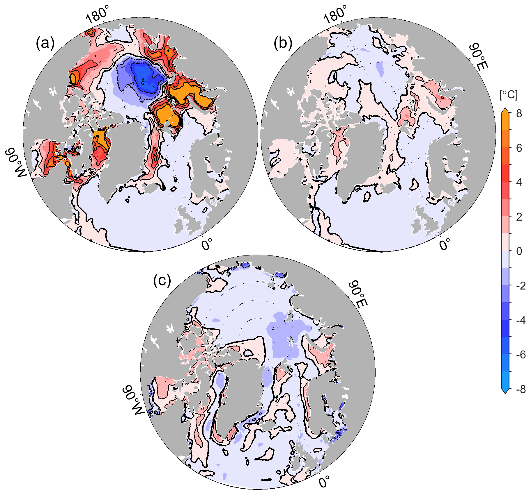
Figure 11 Adjustments of the 2 m air temperature averaged from 20 May to 15 June 2012, in (a) adjoint-FD and (b) adjoint-VP. Panel (c) shows the 2 m air temperature differences between the ERA5 and NCEP-RA1 reanalyses (ERA5 minus NCEP-RA1) averaged from 20 May to 15 June 2012. The contour intervals are 2 ^∘C.

In summary, the two optimization runs successfully reproduce the sea ice retreat process in 2012 by assimilating satellite and in situ measurements. However, the sea ice retreat processes differ in the two optimized simulations, especially from May to June, when Arctic Ocean observations rely mostly on satellite-measured SIC. Considering the amplitude of the 2 m air temperature adjustments, the adjustments of the control variables in adjoint-VP are more reasonable than those in adjoint-FD due to the inclusion of the approximate adjoint of sea ice rheology.

6 Conclusions

The adjoint model is a powerful way to calculate the sensitivities of a target function to model variables and has been applied to coupled ocean and sea ice models for sensitivity studies (Heimbach et al., 2010; Kauker et al., 2009; Koldunov et al., 2013) and state estimations (Fenty and Heimbach, 2013; Koldunov et al., 2017; Lyu et al., 2021b; Nguyen et al., 2021). However, due to the persistent instability issues, the adjoint of sea ice dynamics are traditionally excluded or simplified to the adjoint of free-drift sea ice dynamics, which potentially hampers the accuracy of the coupled ocean and sea ice estimation.

Based on the study of Toyoda et al. (2019) and the coupled ocean and sea ice modeling and adjoint assimilation system (Lyu et al., 2021a), we approximate the adjoint of viscous-plastic sea ice dynamics and test the impacts on estimating the spatiotemporal variations in the Arctic Ocean and sea ice state.

Two optimizations are performed, one including and one excluding the adjoint of sea ice rheology. Both assimilation expriments reduce SIC and SIT errors and reproduce the sea ice retreat well. With the improved SIC retreat processes, adjoint-FD and adjoint-VP also show similar ocean temperature changes in the marginal seas and the southern Beaufort Gyre, as solar radiation heats the open water quickly as the sea ice retreats. With the improved adjoint of sea ice dynamics, adjoint-VP allows much stronger adjustments of the initial temperature, resulting in a more significant improvement on the temperature in the North Atlantic Ocean and the intermediate layer (50–700 m) of the Arctic Ocean.

Although that adjoint-FD computes much stronger sensitivities of the cost function to the wind vectors than adjoint-VP does, we note that adjoint-FD adjusts more (less) of the 2 m air temperature (wind vectors) than adjoint-VP does. It is evident that the adjoint sensitivities of wind vectors in adjoint-FD reduce the cost function less efficiently than those in adjoint-VP during the optimization. Adjoint-FD strongly adjusts the 2 m air temperature to reduce the model–data misfits while adjoint-VP slightly adjusts all the control variables to improve the model simulation.

Using the sea ice budget analysis, we further examine the sea ice retreat processes in adjoint-FD and adjoint-VP. We note that adjoint-FD and adjoint-VP show different sea ice thinning processes from 20 May to 15 June and in the marginal seas. Adjoint-FD destroys the extra sea ice in the marginal seas by substantially increasing the 2 m air temperature (up to 8 ^∘C), which is much larger than the ERA5-NCEP differences. In adjoint-VP, the sea ice thinning is moderate with more reasonable adjustments of 2 m air temperature (within ±3 ^∘C) and the size of the adjustments are much smaller than the ERA5-NCEP differences. Therefore, by including the adjoint of sea ice rheology, adjoint-VP projects the model–data misfits more properly to the control variables than that in adjoint-FD.

Parameter uncertainties significantly impact ocean and sea ice simulations (Lu et al., 2021; Massonnet et al., 2014; Sumata et al., 2019), and a lack of direct observations of key parameters potentially results in biases in the model simulations and predictions. The development of the adjoint of the viscous-plastic sea ice dynamics further introduces three parameters, including the ice compressive strength constant (P^∗), ice strength decay constant (C^∗), and ratio of normal stress to shear stress (e), into the adjoint model. Since it remains unclear how well the tangent linear approximation could represent the relations between the model parameters and the model state, in future studies, we will examine the accuracy of the adjoint sensitivities with respect to the model parameters and then further improve the ocean–sea ice estimations by jointly estimating the state and parameters.