Long-term eddy modulation affects the meridional asymmetry of the halocline in the Beaufort Gyre

Against the background of wind-forcing change along with Arctic sea ice retreat, the mesoscale processes undergoing distinct variation in the Beaufort Gyre (BG) region are increasingly important to oceanic transport and energy cascades, and these changes subsequently put oceanic stratification into a new state. Here, the varying number and strength of eddies in the central Canada Basin (CB) and Chukchi–Beaufort continental slope are obtained based on mooring observations (2003–2018), altimetry measurements (1993–2019), and reanalysis data (1980–2020). In this paper, the variability in the BG halocline, representing the adjustment of stratification in the upper layer, is shown in order to analyse how variability occurs under changing mesoscale processes. We find that over almost the last 2 decades the halocline depth has deepened by ∼ 40 m in the south of the central gyre, while that in the north has deepened by ∼ 70 m according to multiple datasets. Surrounding the central gyre, the asymmetry of the halocline, with much steeper and deeper isopycnals over the southern continental slope, reduced after 2014. In the meantime, eddy activities in the upper layer from the southern margin of the BG to the abyssal plain have been enhanced. Moreover, the convergence of the eddy lateral flux has increased as the halocline structures on either side, which is at least 120 km from the central gyre, have reached a nearly identical and stable regime. It has been clarified that long-term dynamic eddy modulation through eddy fluxes, facilitating the freshwater redistribution, affects the meridional asymmetry of the BG halocline. Our results provide a better understanding of the eddy modulation processes and their influence on the halocline structure.

1 Introduction

Global temperatures have continued to rise since the 1970s. The Arctic Ocean, as the focal point of climate change research, is the region with the most dramatic global surface temperature warming (Huang et al., 2018), with a warming range as high as 1.2 ^∘C per 10 a, more than twice the global average warming range, a phenomenon known as “Arctic amplification” (Serreze and Barry, 2011). These variations not only affect the upper-ocean circulation but also expose the Arctic atmosphere–ice–sea system to rapid changes (Moore et al., 2018; Timmermans and Marshall, 2020). In this context, with summer sea ice declining in the Arctic (Stroeve et al., 2007, 2014; Niederdrenk and Notz, 2018), the presence of increased freshwater in the upper layer alters local stratification, resulting in the variability in water masses. Meanwhile, increased active ocean–atmosphere interactions and mesoscale processes in the Canada Basin (CB) due to the emergence of broader open areas have attracted increasing attention.

The Beaufort Gyre (BG) in the CB, a large-scale wind-driven anticyclonic circulation feature, which stores a substantial amount of freshwater in the CB (Proshutinsky et al., 2009, 2019), is accompanied by prevalent mesoscale eddies (Doddridge et al., 2019; Manucharyan and Spall, 2016; Zhao and Timmermans, 2015; Zhao et al., 2016). The freshwater content (FWC) accumulated by Ekman convergence increased between 2003 and 2008 and remained relatively constant between 2008 and 2012 (Timmermans and Toole, 2023), while in 2013 FWC decreased but increased again from 2014. The halocline in the CB, a thick layer with a double peak of stratification, is considered to be an insulating “density barrier” between the surface mixed layer and the Atlantic water layer underneath (Bourgain and Gascard, 2011). Observations have indicated that the Pacific Winter Water (PWW) layer, the main component of the western Arctic halocline (Shimada et al., 2005), generally deepened during 2004–2018, while the isopycnal layer thickness increased (Kenigson et al., 2021). Likewise, there was an isopycnal deepening of 70 m during 2004–2011 (Zhong et al., 2019), suggesting a spin-up of the gyre. The shape of the BG is highly asymmetrical and is associated with surface forcing (Regan et al., 2019). Furthermore, the asymmetrical stratification and the halocline's vertical structure in the BG have received attention in recent studies (Kenigson et al., 2021; Zhang et al., 2023). Isopycnals are steeper near the gyre edge than in the interior due to the increasing eddy diffusivity via redistributing isopycnal layer thicknesses laterally, indicating stronger baroclinic instability (Manucharyan et al., 2016; Manucharyan and Isachsen, 2019). Isohalines are steeper in the south and east than in the north and west (Zhang et al., 2023). This asymmetrical structure is related to topography, BG strength, and a few other factors that remain to be solved.

Global mesoscale eddies can transmit momentum, heat, and water masses, contributing to atmospheric circulation and mass distribution and playing a role in the ocean heat balance (Chelton et al., 2007). In the Arctic Ocean, eddies have also been observed and analysed in the past. Eddies not only exhibit unprecedented changes but also play a crucial role in the Ekman-driven BG stability in the context of sea ice loss (Manucharyan et al., 2016). They can balance atmosphere–ocean and ice–sea stress inputs, gradually weaken the isopycnal slope and geostrophic currents, and counteract the accumulation of FWC driven by Ekman pumping by dissipating available potential energy (APE) (Manucharyan and Spall, 2016). In addition, Ekman pumping and sea ice are also major factors affecting BG halocline dynamics. This balance between the halocline and eddies is thought to occur on different timescales in realistic models, which suggests a link between small-scale features and changes to large-scale circulation (Doddridge et al., 2019; Manucharyan et al., 2017).

Previous work on eddies has mostly been based on satellite products (e.g. Kozlov et al., 2019; Kubryakov et al., 2021; Raj et al., 2016); in situ hydrographic data (e.g. Fer et al., 2018; Timmermans et al., 2008; Zhao et al., 2014, 2016; Zhao and Timmermans, 2015); and high-resolution, eddy-resolving simulations (e.g. Regan et al., 2020; Wang et al., 2020). As a common feature in the BG halocline, eddies are mainly concentrated in the subsurface (30–300 m), even though they can extend to thousands of metres in depth (Zhao et al., 2014; Zhao and Timmermans, 2015) due to eddy dissipation by ice–ocean drag in the surface boundary layer (Manucharyan and Stewart, 2022). Moreover, the kinetic energy of mesoscale eddy activities is dominant in the BG halocline (Zhao et al., 2016, 2018). For example, based on 127 eddies observed at drifting sea ice stations, Manley and Hunkins (1985) found that the eddy kinetic energy (EKE) accounted for approximately one-third of the total kinetic energy of the upper 200 m in the CB. The depth of the maximal EKE value is generally found at approximately 70–110 m in the halocline (Wang et al., 2020). The southern CB is commonly found with a large number of cold-core and anticyclonic halocline eddies (Spall et al., 2008). Zhao et al. (2016) used ice-tethered profiler (ITP) measurements between 2005 and 2015 to survey the changes in the eddy field in the CB. They found that eddies were mostly distributed in the western and southern parts of the CB. EKE derived by satellites is also higher along the major boundary currents and continental shelves in the Arctic Ocean (Timmermans and Marshall, 2020; Wang et al., 2020).

In this paper, we focus on the long-term variability in eddy activity and associate it with asymmetrical stratification. According to previous work, the number of eddies in the lower halocline doubled from 2005–2012 to 2013–2014 (Zhao et al., 2016), with past increases in FWC and gyre strength before 2007 (Regan et al., 2019; Timmermans and Toole, 2023) and a stabilisation since 2008 (Zhang et al., 2016). The response of EKE to the spin-up of the gyre during 2003–2007 showed that EKE at the subsurface has generally strengthened (Regan et al., 2020). Recent research has also demonstrated that with wind energy input increasing into the BG due to the significant loss of sea ice after 2007, eddy activities would also be more active (Armitage et al., 2020).

However, with sea ice conditions changing due to global warming, research on the long-term variability in eddies in the central basin and basin boundary regions is still limited. Furthermore, according to the standpoints about possible gyre stabilisation and asymmetrical haloclines in recent years (e.g. Proshutinsky et al., 2019; Zhang et al., 2016, 2023), the eddy modulation in the asymmetrical halocline structure is unknown. Here, we use multiple datasets containing moored, in situ, and satellite altimetry observations, in comparison with reanalysis data, to quantify the strength of eddies with sea level anomaly (SLA) and horizontal currents. The stationary eddies and EKE, as well as the variability in the halocline structure, are noted to assess the deformation of the asymmetrical halocline in the BG under the changing eddy modulation. Section 2 presents the details of the data and methodology. Section 3 demonstrates the variability in the entire halocline layer, especially in its meridional asymmetry in the BG region. The eddy distribution and long-term changes are discussed in Sect. 4. Section 5 explains significant eddy modulation in the halocline structure as well as the correlation between EKE and geostrophic currents. Section 6 contains the summary and discussion of this paper.

2 Data and methods

2.1 Observations and ocean reanalysis data

In this paper, we use multiple datasets, including hydrographic observations, satellite altimetry, and reanalysis datasets. The hydrographic data are in situ measurements from conductivity–temperature–depth (CTD) and mooring observations from McLane moored profilers (MMPs) at four moorings that are all deployed under the Beaufort Gyre Exploration Project (BGEP). The reanalysis datasets used here consist of the World Ocean Atlas 2023 (WOA23) and Simple Ocean Data Assimilation (SODA; version 3.4.2).

An annual hydrographic survey has been conducted through ship-based CTD in the BG region each year between August and October. CTD data between 2004 and 2021 are used to investigate the spatiotemporal variability in oceanic stratification across the fundamental BG region (Fig. 1a). The positions of the deployed CTD instruments are shown in Fig. 1b. Additionally, to supplement the long-term trends in and changing characteristics of the halocline and to capture mesoscale eddies at representative stations in the CB, mooring data deployed at four corners around the basin (Fig. 1c) between mid-2003 and mid-2018 above 500 m are also analysed. Each mooring system included a MMP that returns profiles of horizontal velocity, temperature, salinity, pressure, etc. A pair of upgoing/downgoing profiles (separated by 6 h) is returned every other day, and the data are processed to a vertical resolution of 2 dbar. The shallowest moored measurement varies from approximately 50–90 m (depending on the mooring and sampling period) to avoid collisions with ice keels, and the deepest measurements are 2000 m.

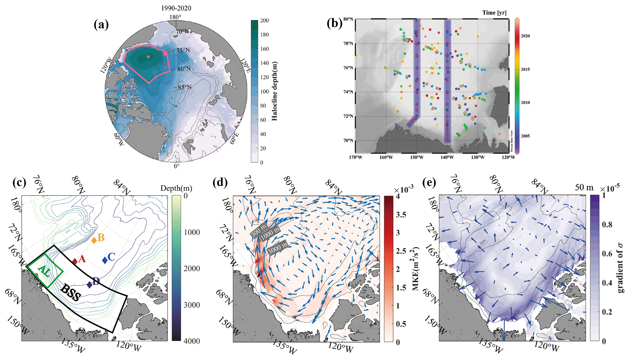
Figure 1 (a) A map of climatological halocline depth. The area surrounded by the pink line and the star indicate the BG area and its centre, respectively (Regan et al., 2020). This BG box is defined as the region between 70.5–80.5^∘ N and 170–130^∘ W, bounded by the 300 m bathymetry. The centre of the mean gyre from 1990 to 2014 is situated at 74.74^∘ N and 150.62^∘ W. (b) The positions of the in situ sites of CTD measurement from BGEP in certain months during 2004–2021. The purple bars indicate two meridional transects with a width of 36 km mostly along 150 and 140^∘ W. (c) A map of the Canada Basin and the bathymetric contours above the 4000 m isobath. The coloured diamonds denote the locations of four BGEP moorings. The two chosen regions are shown by green (Alaskan coast, AL) and black (Beaufort Sea slope, BSS) boxes. (d) The distribution of the mean kinetic energy (MKE) at 50 m. The vectors denote the direction of the mean currents. The grey lines denote the 300, 1000, and 3000 m bathymetries. (e) The distribution of the horizontal gradient of potential density (shading) at 50 m. The vectors point in the direction of increasing potential density. The results of (a), (d), and (e) are calculated from the 1990–2020 WOA climatology.

The SODA reanalysis has been developed by the University of Maryland based on the Global Simple Ocean Data Assimilation System, which is the 5 d average from 1980 to 2020 adopted in this paper, with a horizontal resolution of $\mathrm{1}/\mathrm{2}$^∘ × $\mathrm{1}/\mathrm{2}$^∘ and 50 vertically divided layers with unequal spacing. We obtained gridded altimetry data (product identifier: SEALEVEL_GLO_PHY_L4_REP_OBSERVATIONS_088_047) over the years 1993–2019 from the Copernicus Marine Environment Monitoring Service (CMEMS). This product consists of daily gridded maps of dynamic topography in ice-free regions that have been derived as the sum of mapped SLAs calculated from combined measurements by different satellites and mean dynamic topography (MDT) (Kubryakov et al., 2021).

2.2 Methods

To estimate EKE and assess the strength of eddy activities, we use ocean current data from SODA and altimetry. Geostrophic velocities are calculated from sea level height. The horizontal velocity is deconstructed into the annual mean velocity $\left(\stackrel{\mathrm{‾}}{u}\stackrel{\mathrm{‾}}{v}\right)$ and anomaly $\left(u^{\prime }{v}^{\prime }\right)$ as follows (Penduff et al., 2004; Rieck et al., 2015, 2018; Regan et al., 2020):

$$u=\stackrel{\mathrm{‾}}{u}+u^{\prime },u=\stackrel{\mathrm{‾}}{v}+v^{\prime },$$

and subsequently

$$\begin{array}{}\text{(1)}& \mathrm{EKE}=(u^{\prime \mathrm{2}}+v^{\prime \mathrm{2}})/\mathrm{2}.\end{array}$$

Note that the EKE in this paper is estimated by a low-frequency eddy, which is defined as the departure from a long-term temporal mean, with a period (depending on the temporal resolution of the data) of greater than 5 or 1 d (Luecke et al., 2017). In addition, the vertical velocity shear $\partial \mathbf{U}/\partial z$ can be related to the large-scale density field by the thermal wind relation:

$$\begin{array}{}\text{(2)}& {\displaystyle \frac{\partial \mathbf{U}}{\partial z}}={\displaystyle \frac{g}{f_o{\mathit{\rho }}_o}}{\displaystyle \frac{\partial \mathit{\rho }}{\partial z}}\mathit{k}\times \mathrm{\nabla }{z}_{\mathit{\rho }}={\displaystyle \frac{N^{\mathrm{2}}}{f_o}}\mathit{k}\times \mathrm{\nabla }{z}_{\mathit{\rho }},\end{array}$$

where U is the horizontal current field; N is the Brunt–Väisälä buoyancy frequency, which represents oceanic stratification; $\mathrm{\nabla }{z}_{\mathit{\rho }}=(-\frac{\partial \mathit{\rho }}{\partial x}/\frac{\partial \mathit{\rho }}{\partial z},-\frac{\partial \mathit{\rho }}{\partial y}/\frac{\partial \mathit{\rho }}{\partial z})$ is the isopycnal slope; ρ is the potential density of seawater; ρ_o is the average density of seawater; g is the gravity acceleration; and z is depth (Meneghello et al., 2021). Developed by Eq. (2), the horizontal velocity field is calculated by integration with depth from the bottom to the surface. As shown by the maps of the horizontal velocity field (Fig. 1d) and density gradient (Fig. 1e) at 50 m in the CB, the main circulation feature is discerned, and the southwestern basin near the continental slopes is the key region for varying currents tending towards high EKE and instability.

To investigate the variation in the overall halocline and understand the shifting in oceanic stratification, we consider the depth of the potential density surface σ=27.4 (25) kg m⁻³ to approximately represent the base (top) of the entire halocline layer (Timmermans et al., 2020). Accordingly, the depth of the surface mixed layer is also identified by the halocline upper boundary (Bourgain and Gascard, 2011; Polyakov et al., 2018). Based on the upper and lower boundaries of the halocline, APE is defined as the amount of potential energy in a stratified fluid available for mixing and conversion into kinetic energy (Huang, 1998; Munk and Wunsch, 1998). Here, the calculation of APE follows Eq. (3):

$$\begin{array}{}\text{(3)}& \mathrm{APE}=\mathrm{PE}-{\mathrm{PE}}_{\mathrm{ref}}=\underset{z_{\mathrm{ref}}}{\overset{\mathrm{surface}}{\iiint }}g[\mathit{\rho }\left(z\right)-\mathrm{1027.4}]z\mathrm{d}z\mathrm{d}A,\end{array}$$

where z_ref represents the depth of the halocline lower boundary, and A is the gyre area (Armitage et al., 2020; Bertosio et al., 2022; Polyakov et al., 2018).

Furthermore, to discern the critical role of mesoscale eddies in balancing the halocline, we consider that the eddy advection velocity in the y–z plane can be defined from an eddy stream function ψ^∗ as

$$\begin{array}{}\text{(4)}& v^{\ast }=-{\mathit{\psi }}_z^{\ast },w^{\ast }={\mathit{\psi }}_y^{\ast },\end{array}$$

and ψ^∗ is represented as

$$\begin{array}{}\text{(5)}& {\mathit{\psi }}^{\ast }={\displaystyle \frac{\stackrel{\mathrm{‾}}{v^{\prime }{S}^{\prime }}}{\stackrel{\mathrm{‾}}{S_Z}}}=-{\displaystyle \frac{\stackrel{\mathrm{‾}}{w^{\prime }{S}^{\prime }}}{\stackrel{\mathrm{‾}}{S_y}}},\end{array}$$

where $\stackrel{\mathrm{‾}}{v^{\prime }{S}^{\prime }}$ is the average meridional eddy salt flux, and $\stackrel{\mathrm{‾}}{S_Z}$ is the average vertical salt gradient (Manucharyan et al., 2016; Manucharyan and Spall, 2016; Manucharyan and Isachsen, 2019; Marshall and Radko, 2003). Here, bars and primes correspond to the annual mean and perturbation variables. Because buoyancy is mainly controlled by salinity in the Arctic, ψ^∗ represents the cumulative effects of eddy thickness fluxes that arise from correlations between eddy velocities and eddy-induced isopycnal displacements. Overall, when the vertical salt gradient is generally negative in the CB, a positive value of ψ^∗ indicates southward eddy thickness fluxes and vice versa.

If the eddy genesis is related to baroclinic instability, the baroclinic growth rate ω is correlated with EKE. The baroclinic growth rate ω can be estimated here by

$$\begin{array}{}\text{(6)}& \mathit{\omega }=f\sqrt{{\displaystyle \frac{\mathrm{1}}{\mathrm{6}H}}\underset{H}{\overset{\mathrm{0}}{\int }}{\displaystyle \frac{\mathrm{d}z}{\mathit{Ri}\left(z\right)}}},\end{array}$$

where $\mathit{Ri}=N^{\mathrm{2}}/\left[{\left(\frac{\partial u}{\partial z}\right)}^{\mathrm{2}}+{\left(\frac{\partial v}{\partial z}\right)}^{\mathrm{2}}\right]$ is the Richardson number (Smith, 2007). We call the inverse of this quantity ${\mathit{\omega }}^{-\mathrm{1}}=T$ quantity the “Eady timescale”. The Eady timescale should be short where there is anomalously high EKE or weak stratification.

3 BG halocline variability

In this section, we aim to investigate the spatiotemporal variability in the halocline in the BG region, particularly its varying asymmetry inside, which is the focus of this article. The halocline's depth, thickness, strength, and vertical structure are analysed in detail below, all of which indicate its meridional asymmetry.

3.1 Temporal variation in the halocline

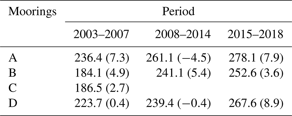
With the spin-up of the BG, the isopycnals of the PWW layer in the cold halocline deepen (Kenigson et al., 2021). We chose the 25 and 27.4 kg m⁻³ isopycnal surfaces to characterise the halocline top and base. Figure 2 shows the temporal variation in the depth of the halocline upper and lower boundaries and halocline thickness at four moorings from MMP combined with CTD. The depth of the surface mixed layer is less than 70 m. The entire halocline layer underneath the mixed layer, including the upper and lower halocline boundaries, is mainly at 70–250 m. Compared with the MMP results, the mean relative errors in CTD with respect to the halocline base depth are 2.6 %, 3.6 %, and 1.3 % for moorings A, B, and D, respectively. Given that the rangeability of the halocline top is much smaller than that of the halocline base, we mainly focus on the variation in the halocline base. There are different characteristics of variation in the halocline depth during 2003–2018, despite a lack of measurements over time. The MMP results at mooring C showed a deepening trend in the halocline depth before 2008, overlapping well with mooring B. In addition, other moorings provided results over a longer term, which captured a deepening of the halocline base and an increase in thickness over the years 2003–2018. The thickness of the halocline at mooring B in the northwestern part of the CB increased steadily by approximately 70 m; moreover, the depth of the halocline base deepened by up to 70 m over the years 2003–2018. The thickness of the halocline in the southern part of the basin (moorings A and D) increased by approximately 30 m with the halocline base deepening by approximately 40 m. Notably, the depth of the halocline base had a stagnant phase and even shallowing development over the years 2008–2014. The linear trends in and mean values of the halocline depth over three periods (2003–2007, 2008–2014, and 2015–2018) are computed (Table 1). A shallowing trend in halocline depth is clear during 2008–2014 in the southern sites of the basin (moorings A and D), but both the former and the latter periods mostly exhibit deepening trends in halocline depth. The variations in northern regions (moorings B and C) covering three periods are similar, which show entirely different features from southern regions. The halocline depth continues to deepen over the whole period. The halocline thickness and depth between every site tend to be at a nearly identical level in the final period, and those differences are smaller than in the first period.

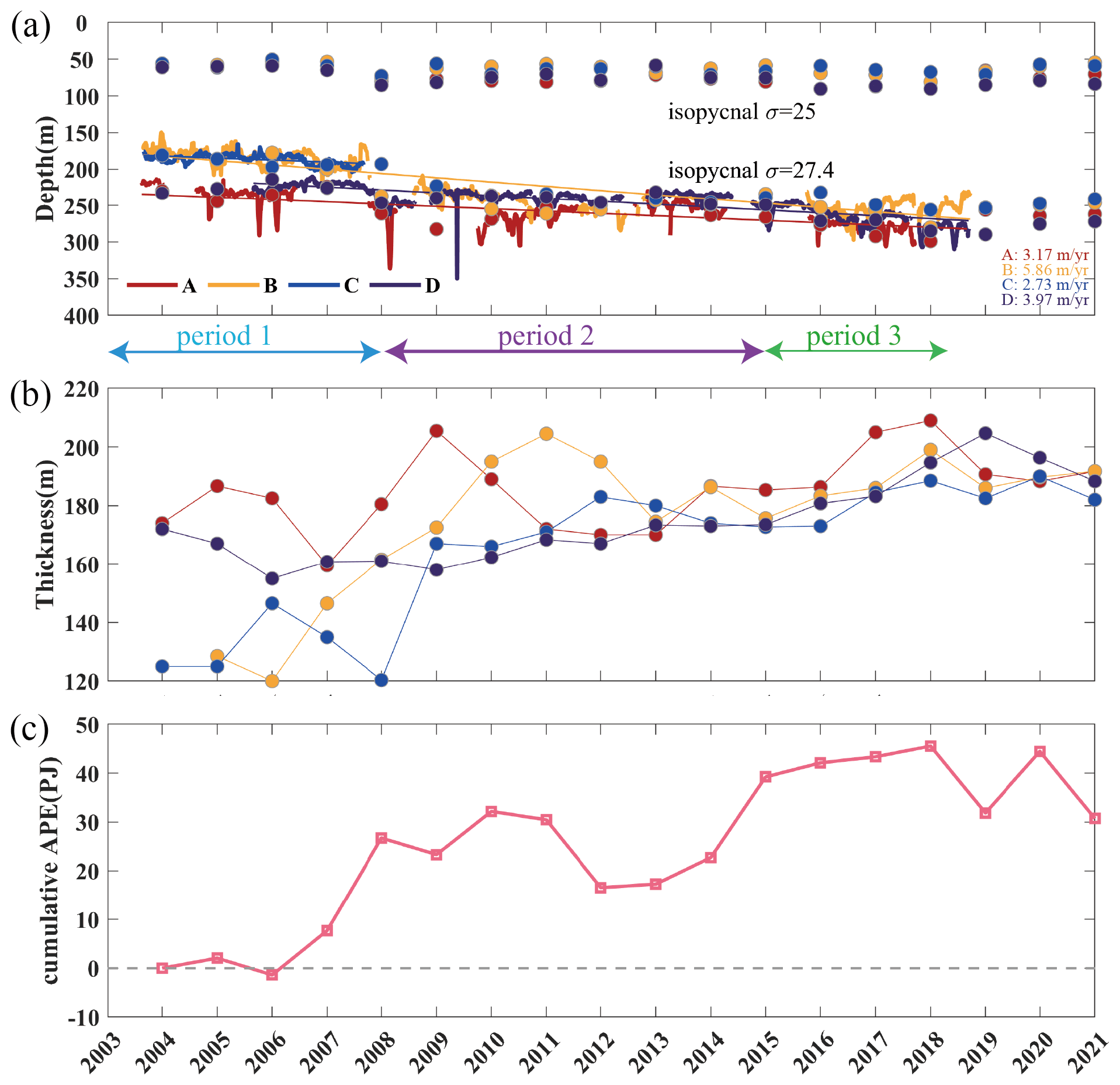
Figure 2 Time series of (a) the depth of the 25 (upper coloured lines) and 27.4 kg m⁻³ (lower coloured lines) isopycnals representing the top and base of the halocline at the positions of moorings A, B, C, and D based on MMP (solid lines) and CTD (dots). The long-term deepening trends in the depth of the halocline base from MMP are marked. Note that the anomalies record eddies that were existent at that time. (b) Annual variability in halocline thickness between the 25 and 27.4 kg m⁻³ isopycnals from CTD. (c) Annual variability in accumulative APE in the BG box calculated from CTD.

APE, a good integral indicator of changes in overall halocline strength in the BG box, is also computed here by Eq. (3) using CTD surveys. As shown in Fig. 2c, APE had accumulated ∼ 30 PJ up to 2008. However, APE continuously decreased in the 2010–2012 period and remained at a relatively low level in 2012–2013, pointing to a flattening of isopycnals in the BG and APE release. Although there was a significant short-term increase in 2014–2015, moderate accumulation occurred in 2015–2018, indicating a saturation of the accumulative energy reservoir of around 40–50 PJ. We infer the variabilities in the halocline and APE have a relationship with the BG spin-up and the largest increase in FWC during 2003–2007 (Giles et al., 2012; Krishfield et al., 2014; Timmermans and Toole, 2023). Additionally, halocline depth and thickness remained stagnant in the post-spin-up term during 2008–2014 (Regan et al., 2020).

Table 1 Trends (within the brackets, unit: m yr⁻¹) that all pass significant tests (99 % confidence level) and mean depth (outside the brackets, unit: m) of the halocline base over three periods for moorings A, B, C, and D.

3.2 Changes in the meridional asymmetry of the halocline

The stratification in the BG region is marked by pronounced asymmetry, as highlighted by Zhang et al. (2023). The isopycnal slope is steeper over the southern continental slope than in the northern basin (Fig. 1e), which is in line with previous research (e.g. Proshutinsky et al., 2019; Regan et al., 2019; Zhang et al., 2023). In Sect. 3.1, we observe that there are significant differences in the evolution of the halocline between the northern and southern parts of the basin. Earlier research has also showed that the largest deepening of the 27 kg m⁻³ isopycnals occurred in the northwestern and northeastern regions during 2002–2016 (Zhong et al., 2019). Our analysis also reveals a more noticeable meridional difference between the north and south. To gain a comprehensive understanding of the asymmetric halocline across the fundamental BG box, we utilise inhomogeneously gridded in situ hydrographic data from the latest CTD survey (Fig. 1a). The data are optimally interpolated onto a regular grid with a grid spacing of 1^∘ in longitude and 0.5^∘ in latitude. By examining the horizontal maps in three distinct periods (Fig. 3), based on the trends in halocline depth at the moorings, we see evident changes in the horizontal patterns of the halocline depth. This suggests a transformation of oceanic stratification in the upper layer. In the initial period, the halocline base maps highlight significant differences between the north and south. The north then experiences a much more pronounced deepening of the halocline depth compared to the south closer to the Beaufort Sea slope, which also exhibits more freshwater. In the final period, the areas with the maximal halocline depth, which are located in the abyssal plain between the Canadian Arctic Archipelago and Northwind Ridge, enlarge.

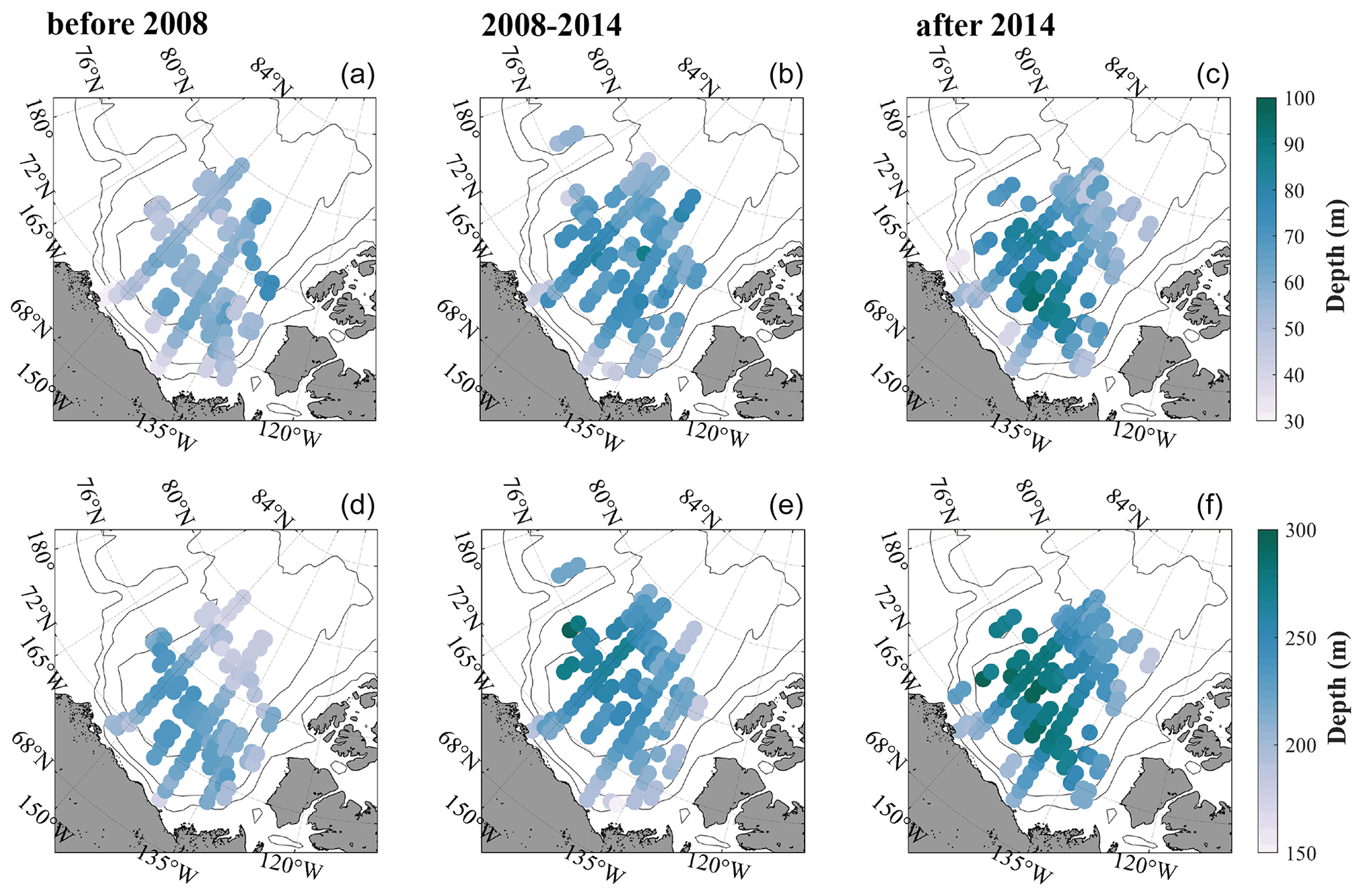
Figure 3 Horizontal distribution of the depth of the halocline (a–c) top and (d–f) base over the Beaufort Gyre region averaged in 2004–2007 (before 2008), 2008–2014, and 2015–2021 (after 2014).

According to the movements of the gyre centre, mainly between 140 and 150^∘ W over 2003–2014 (Regan et al., 2019), we select two north–south transects along 140 and 150^∘ W (Fig. 1b), which both traverse the deepest part of the BG halocline (Fig. 1a), and make a comparison. There is variability based on different transects in every period, which demonstrates the spatial difference in the BG halocline layer. Although the sections can not capture the same portion of the gyre over three periods, we find that the hydrographic structures and deformation from the two transects have similar features (Fig. 4), which is the same as a former study (Timmermans and Toole, 2023). From the view of the two transects, the halocline thickness was relatively thicker in the south than in the north before 2008. However, the change is more significant and the halocline layer is much thicker along 150^∘ W than along 140^∘ W. Thus, we emphasise the shifts in the halocline structures along the 150^∘ W transect. The vertical distributions of the σ=27.4 kg m⁻³ isopycnal surface show that it is the shallowest (∼ 200 m) at the margins of the BG region and up to 80 m deeper in the interior in the final period (Fig. 4). Based on SODA reanalysis, we considered the impact in the north of the BG extent and put the halocline structure to the north beyond the BG box into comparison. The isopycnal fluctuation in the halocline is remarkable just south of approximately 82^∘ N but negligible far from the BG region (Fig. S1 in the Supplement and Fig. 4c). The much steeper isopycnal slope near about 90^∘ N is due to an overall weakening stratification in the Eurasian Basin that is different from that in the CB. In the BG box, where the halocline is the deepest and its slope is obvious, variability in the main part of the BG halocline is well captured in spite of the northern limit of observation.

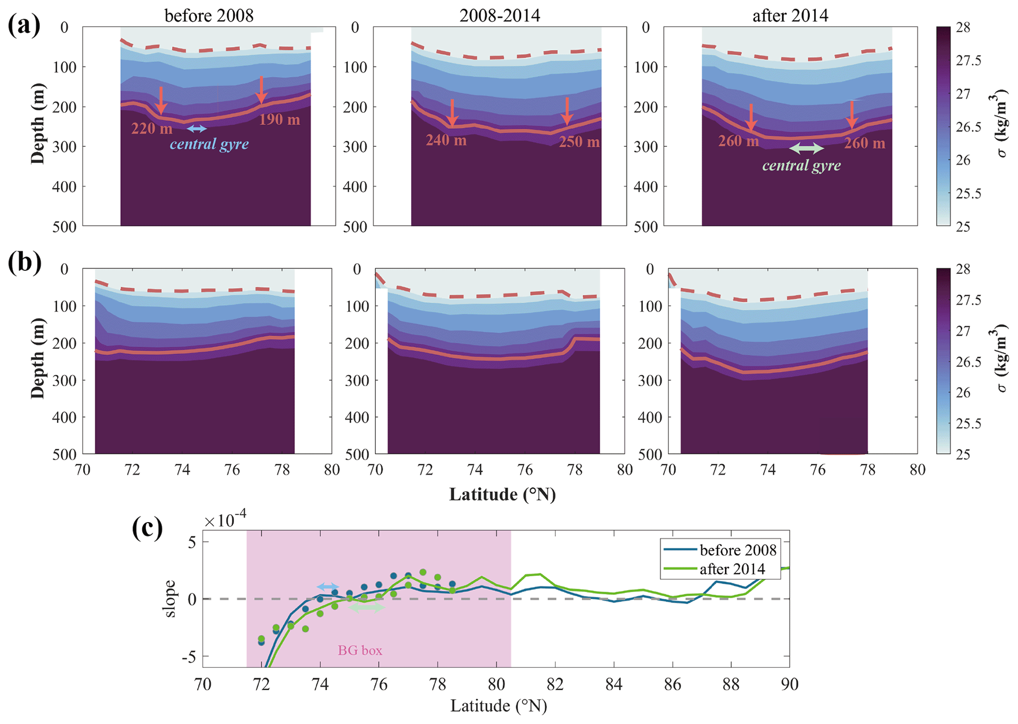
Figure 4 Vertical transects along (a) 150^∘ W and (b) 140^∘ W of the interannual mean potential density using data from CTD measurements in 2004–2007 (before 2008), 2008–2014, and 2015–2021 (after 2014). The dashed (solid) lines indicate the depth of σ=25 (27.4) kg m⁻³ representing the halocline top (base). The depths of the halocline base on either side, which is at least 120 km from the central gyre, are marked in (a). (c) Meridional slope of the σ=27.4 kg m⁻³ isopycnal in the first and last periods from SODA (solid lines) and CTD (dots).

Among the three periods, the vertical structures of the isopycnals, especially the lower boundary of the halocline layer, reveal apparent changes between the marginal and interior gyre. Initially, the location of the central gyre, determined by an isopycnal slope of nearly zero in the interior, was in the vicinity of continental slopes, with the largest isopycnal steepening occurring on the southern side and stronger baroclinic instability (Manucharyan and Isachsen, 2019). In the first period, there was a gradual uplift of the halocline beyond the northern edge of the BG. The obvious meridional symmetry in the halocline can be explained by the intrusion of Atlantic water and strong Ekman downwelling in the central BG (Karcher et al., 2007; McLaughlin et al., 2004; Timmermans and Toole, 2023). The halocline depth on either side, which is taken between the gyre edge and its centre, is in particular compared over three periods. The depth of the halocline base was deeper by approximately 30 m, and the halocline layer was thicker in the southern side (∼ 73^∘ N), more than 120 km from the central gyre, than in the northern side (∼ 77^∘ N). The difference between the north and south was narrowed with isopycnals generally deepening from the view of the average vertical structure during 2008–2014, and even the northern halocline was deeper than the southern district. In the final period (after 2014), the halocline depth changed less in comparison with the previous period. The location of the BG centre moved to the north, which was supported by observations and SODA reanalysis (Fig. 4c). With the northward movement, more southern areas of the BG are not as affected by the limitation of continental slopes. The steeper halocline occurred on the northern side of the central gyre. In the meantime, with more areas of little halocline steepness surrounding the gyre centre than before, the entire halocline layer inflated (Zhang et al., 2023), corresponding with stable development in the APE of the BG system after a significant accumulation (Fig. 2c). Additionally, the halocline depth and thickness tended to be meridionally symmetrical, accompanied by a flattened isopycnal slope surrounding the central gyre, shaped like a horizontal bowl under the forcing of surface Ekman convergence (Manucharyan and Spall, 2016), indicating that it had reached a state of stabilisation (Zhang et al., 2016). As seen from the spatial maps and vertical structures of the halocline, meridional asymmetry reduced in the final period. We infer there are other physical processes contributing to the variability.

4 Spatiotemporal variability in eddy activity

As revealed in previous research, a regime shift in the BG occurred in 2007–2008, with a spin-up phase of the gyre from 2003 to 2007 and stabilisation after 2007 (e.g. Regan et al., 2020; Zhang et al., 2016). With BG spin-up and regional sea ice retreat, mesoscale eddies respond in order to dissipate extra energy input and influence the energy redistribution (Armitage et al., 2020). It is speculated that the eddy genesis is related to APE accumulation and release in the BG region, which can influence the vertical structure of the internal halocline (Manucharyan and Spall, 2016; Manucharyan et al., 2016). In the final period, the developments of meridional asymmetry in the halocline layer and APE within the BG box have been inhibited. Against this background, the spatiotemporal variability in eddy activity, needed for a comprehensive understanding, is discussed in this section.

4.1 Eddy detection and variation

We outline how mesoscale eddies can be detected based on moored observations. When eddies occur locally, there are strong horizontal velocities accompanied by isopycnal displacements. For anticyclonic (cyclonic) eddies, the isopycnals are convex (concave). We distinguish horizontal speeds larger than 10 cm s⁻¹ after removing background currents and isopycnal displacements, both of which are criteria used in the literature (Timmermans et al., 2008; Zhao et al., 2014; Zhao and Timmermans, 2015). All in all, 37, 40, 7, and 43 eddies are detected above 500 m at moorings A–D, respectively. Similar to previous work (e.g. Zhao et al., 2014; Zhao and Timmermans, 2015), in most instances, the temperature/salinity anomalies and convex isopycnal displacements in the eddy core are pervasive. Cold-core eddies account for 61.4 %. A total of 98 % of eddies are anticyclones, and only three eddies detected at mooring C are cyclones. The cold-core anticyclones are common in the BG region due to large-scale dominant anticyclonic circulation coupled with oceanic stratification, where cold and fresh Pacific water overlies warm and salty Atlantic water. Furthermore, for mooring C, which is less controlled by the BG, with weaker mean flows (Fig. 1), the characteristics of eddies are different from others. Some of the eddies are cyclones that are seldom discovered at other moorings. Cyclone existence is related to frontal instability near 80^∘ N, which contributes to cyclone formation (Manucharyan and Timmermans, 2013; Timmermans et al., 2008).

In addition, we confirm the annual mean days of existing eddies and the number of warm-core and cold-core eddies over 500 m through moored observations. The interannual variations in the days of recording mesoscale eddies and the number of eddies are highly similar at moorings A and B, and several respective peaks are predominant (Fig. 5, the days of effective observations exceed 200 d in most eddy-rich years). The days of eddy activities demonstrate considerable interannual fluctuations. Over the whole period, 2005, 2010, and 2017 are eddy-rich years for mooring A; for mooring B, 2005, 2009, and 2018 (144 d record valid observations) are eddy-rich years, which is affected by the spatial inhomogeneity in eddy distribution or eddy transport from the southern BG region (Armitage et al., 2020), the key area for eddy generation (Kubryakov et al., 2021; Manucharyan and Isachsen, 2019; Zhao et al., 2014). After 2014, eddy activities at mooring A (B) were more active than in the medium period of 2011–2014 (2010–2014) when there was a trend of decreasing eddy days. Despite the eddy days for mooring D showing a smaller fluctuation than other moorings, the amplitude of the eddy number is noticeable. The in situ measurements at mooring D also capture a considerable number of mesoscale eddies, with a trend of decreasing eddy numbers during the medium term of 2009–2014, in line with other moorings.

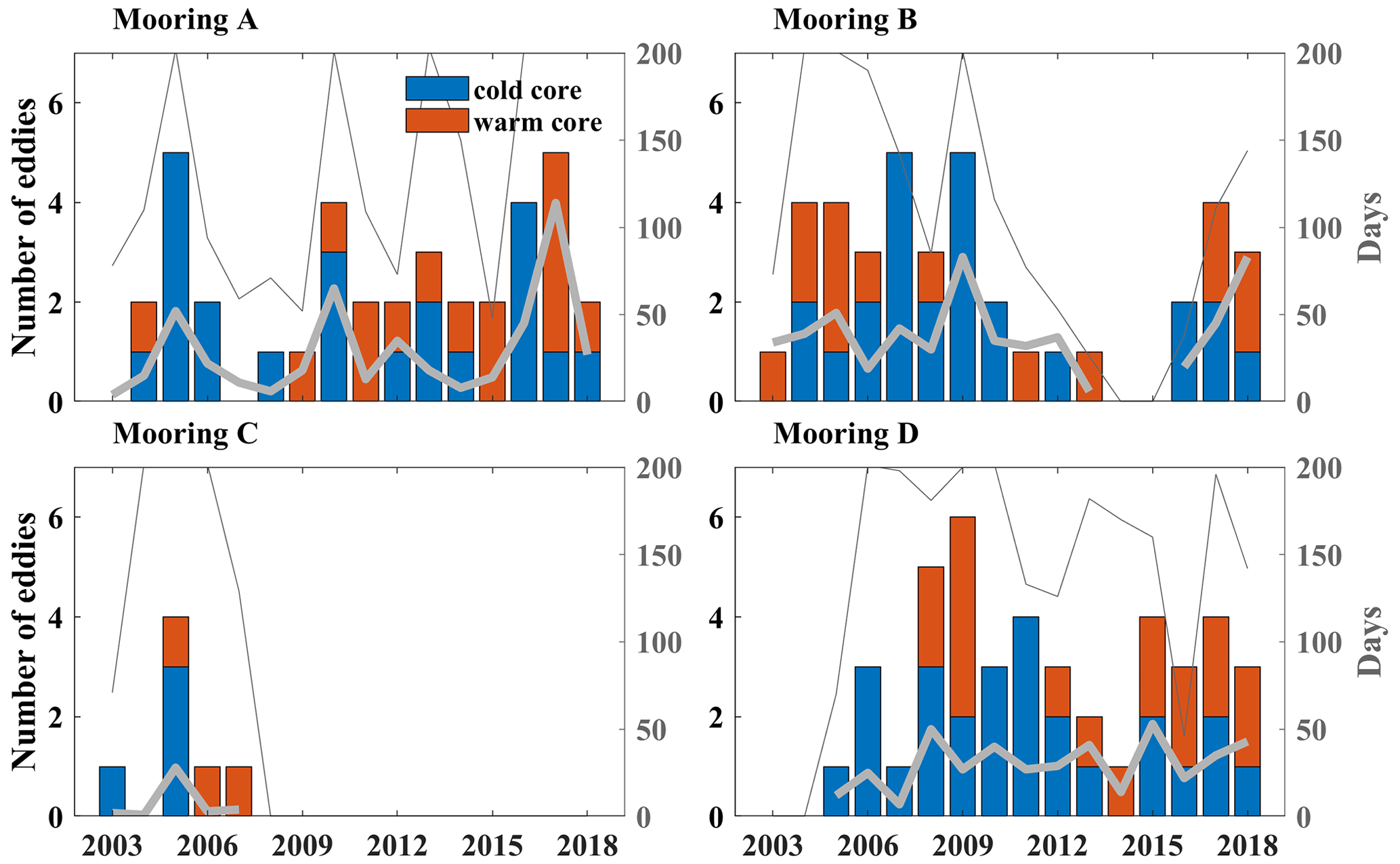
Figure 5 Interannual evolution of the days of existing eddies (thick grey line) and number of eddies (bar) for four moorings. The blue and orange bars indicate the number of cold-core and warm-core eddies, respectively. The thin grey lines signify the days of recording valid observations in every year.

Eddies are common between the upper and lower halocline boundaries (Fig. 6a). Additionally, comparing EKE along with the kinetic energy of individual eddy (KE_eddy) profiles in three periods at the moorings, KE_eddy accounts for ∼ 50 % of EKE (Fig. 6b). EKE, as a measurement of eddy strength, can replicate the main feature of KE_eddy profiles well. EKE changes significantly above the halocline in the three periods, while below the halocline layer, it is relatively weaker, and its multiyear variation is much smaller. The vertical structures of EKE in the basin and its marginal seas can be classified into two types. The first type is that EKE is up to ∼ 0.01 m² s⁻² under the surface mixed layer and decays with depth. The second type is with a maximum value at the subsurface of approximately 70–250 m between the upper and lower halocline boundaries. In the first period, EKE above the BG halocline remained at a relatively low level. The results from three moorings, A, B, and D, showed that EKE was strengthened to varying degrees, accompanied by a deepening of the halocline lower boundary. At the southwestern corner (mooring A) of the basin, only three eddies were detected in the first period. EKE increased in the second period when there were 15 eddies and remained stable in the third period with 13 eddies. The northwestern (mooring B) EKE, with 14 eddies, was stronger in the second period than before, despite the detection of 17 eddies in 2003–2007. EKE was weaker in the third period due to fewer observations. The southeastern (mooring D) EKE did not show apparent growth until the third period due to much stronger eddies detected. There were only 14 eddies detected in 2014–2018 and 24 eddies in 2008–2014. In short, there were either stronger eddies or more eddies after 2014 than before.

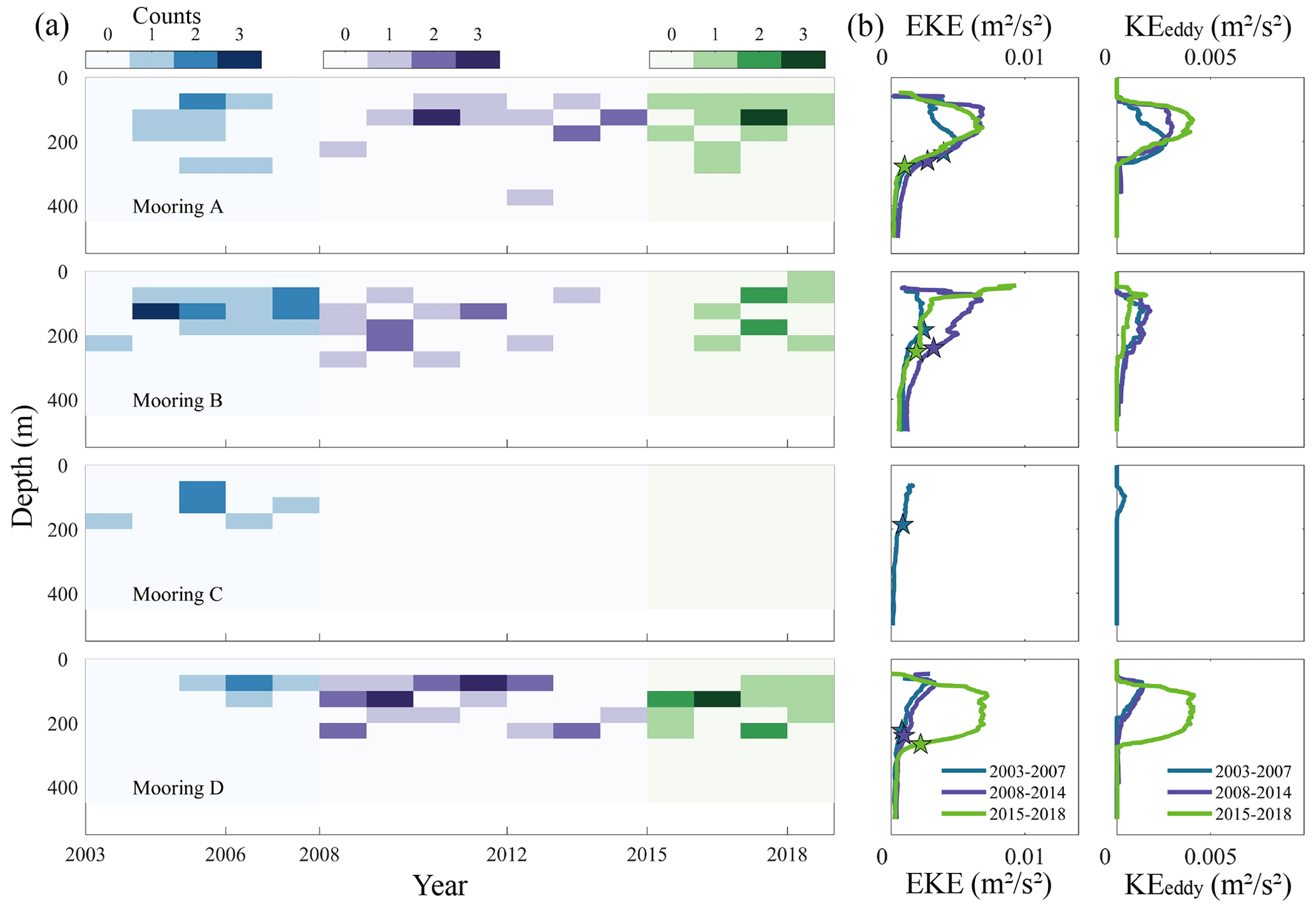
Figure 6 (a) Hovmöller diagrams of depth against time showing annual eddy counts in the upper layer at moorings A–D. Blue, purple, and green shadings denote the spans of the three periods. (b) Interannual mean vertical profiles of eddy kinetic energy (EKE) and kinetic energy from eddies (KE_eddy). The coloured stars indicate the depths of the halocline base in the corresponding periods.

4.2 Long-term EKE evolution from multiple datasets

The BG region, a focal area for mesoscale phenomena in previous studies (Armitage et al., 2020; Regan et al., 2020; Zhao and Timmermans, 2015; Zhao et al., 2016), mainly consists of a southern narrow continental shelf close to the Alaskan coast and a sizable deep basin. The Chukchi–Beaufort slope is a major sector of eddy generation by baroclinic instability (Spall et al., 2008), with a surface front approximately along the 300 m isobath (Timmermans and Toole, 2023), and then eddies carrying Pacific water propagate to the central BG by the boundary current. Here, we focus on this area to investigate the interannual mean surface EKE patterns from a broad perspective with satellite-derived dynamic heights. As shown in Fig. 7, the high-value areas of EKE are mainly located along the continental slopes of the marginal CB, especially the Alaskan coast, mostly between the 1000 and 3000 m isobaths. Indeed, energy is the strongest at the southwestern shelf break of the CB near the Barrow Cape, which can reach more than $\mathrm{5}\times {\mathrm{10}}^{-\mathrm{3}}$ m² s⁻², while it is even less than $\mathrm{1}\times {\mathrm{10}}^{-\mathrm{3}}$ m² s⁻² in the interior basin. Notably, the horizontal pattern of EKE is not identical to that of mean kinetic energy (MKE) obtained by the annual mean geostrophic current. Overall, the area with the highest EKE is closer to the inshore shelf seas than the area with the highest MKE. Along the Alaskan coast (south of 72^∘ N), EKE is higher than MKE by approximately 1 order of magnitude, indicating EKE is dominant in this region, while in the offshore deep basin, MKE is 1 order of magnitude higher than EKE, which agrees with most areas in the Arctic Ocean (von Appen et al., 2022). In every period, the EKE field along the southern continental slope was significantly enhanced compared with that in the previous period, and the strong EKE gradually developed from coasts to offshore regions and the central basin with time. For instance, from the interannual mean horizontal patterns, the region with the strongest EKE was mostly concentrated at the southern part of 72^∘ N if we only look at the section along the 1000 m isobath before 2007 (1993–2007), and it extended to approximately 73^∘ N in the next period. Furthermore, the domain was extended even northwards up to 74^∘ N at the Northwind Ridge, delineated by a long, clear, and curved ribbon in the final period. Particularly, EKE was comparable with MKE near the central BG after 2014. We imply that eddy enhancement and transport contribute considerably to this development, which still needs additional evidence.

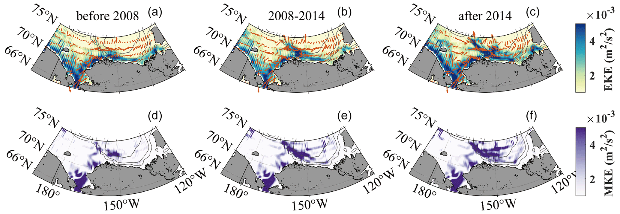
Figure 7 Interannual mean maps of (a–c) eddy kinetic energy (EKE) and (d–f) mean kinetic energy (MKE) at the surface in 1993–2007 (before 2008), 2008–2014, and 2015–2019 (after 2014). The geostrophic current field is indicated by the vectors.

Currently, the seasonality of EKE in the Arctic is clear – generally stronger in summer or autumn and weaker in spring or winter (Wang et al., 2020; Manucharyan and Thompson, 2022) – which is similar to other global regions (Rieck et al., 2015; Jia et al., 2011). The seasonal cycles of EKE in the central basin and basin boundary regions are all distinct (Fig. 8b). However, research on long-term EKE evolution is still limited. The Alaskan coast and the Chukchi–Beaufort slope are the key areas of varying EKE (Fig. 7). In addition, we use datasets derived from SODA reanalysis, altimetry, and moored observations to explore the long-term variability in EKE between the central basin and continental slope. We select a western point of the Alaskan coast called the AL region near the Barrow Cape (Fig. 1c) and the BG region represented by the positions of four moorings. As shown in the eddy detection from MMP, eddies are common in the upper and lower halocline of the CB (Zhao et al., 2014). The variability in eddy counts in four moorings is also consistent with former research by ITP observations in four sectors of the CB (Zhao et al., 2016), so EKE above the halocline base for different moorings is vertically averaged with depth to comprehensively characterise the main features of eddy strength over the years between 2003 and 2018.

Based on previous work, surface eddy activities directly respond to the extra wind energy input (Armitage et al., 2020), while the subsurface EKE is related to baroclinic instability and APE release (Manucharyan and Spall, 2016; Manucharyan et al., 2016). Eddy activities at both the surface and the subsurface are linked with BG stabilisation, contributing to increased energy dissipation. Here the annual mean time series of surface EKE from SODA reanalysis (1980–2020) and altimetry (1993–2019) in the AL region and subsurface EKE from MMP (2003–2018) in the BG region are compared (Fig. 8). There were more missing data before 2003 and relatively low APE within the BG region initially, so we do not discuss it emphatically. EKE from altimetry has increased gradually since the 1990s and peaked in 2009, after which it decreased in 2009–2010, resulting in relatively weak and stable EKE in 2010–2015. Although the EKE from reanalysis is higher than the measurement techniques, it has also increased since the 1990s and remained at a relatively stable level in 2010–2013. In the BG region, subsurface EKE began to increase rapidly from 2003 and peaked in 2009, and it decreased until 2014, which was slightly different from that in the AL region. When EKE was relatively strong after increasing, its cumulative effect contributed to the plateauing of the halocline depth and weakening of the halocline steepness associated with APE release. These characteristic shifts in eddy and oceanic stratification were both related to the varying physics of the gyre in the upper layer that indicated a strengthening during the years before 2007 and a possible stabilisation since 2008 (Zhang et al., 2016). After experiencing a low ebb, especially from altimetry and MMP, since 2014/15, EKE has presented some enhancements over time and has remained at higher levels than in previous years before 2008 between the central BG and marginal AL regions. Based on the three datasets, the strength of eddy activity remained at a relatively higher level in the final period than in the first period.

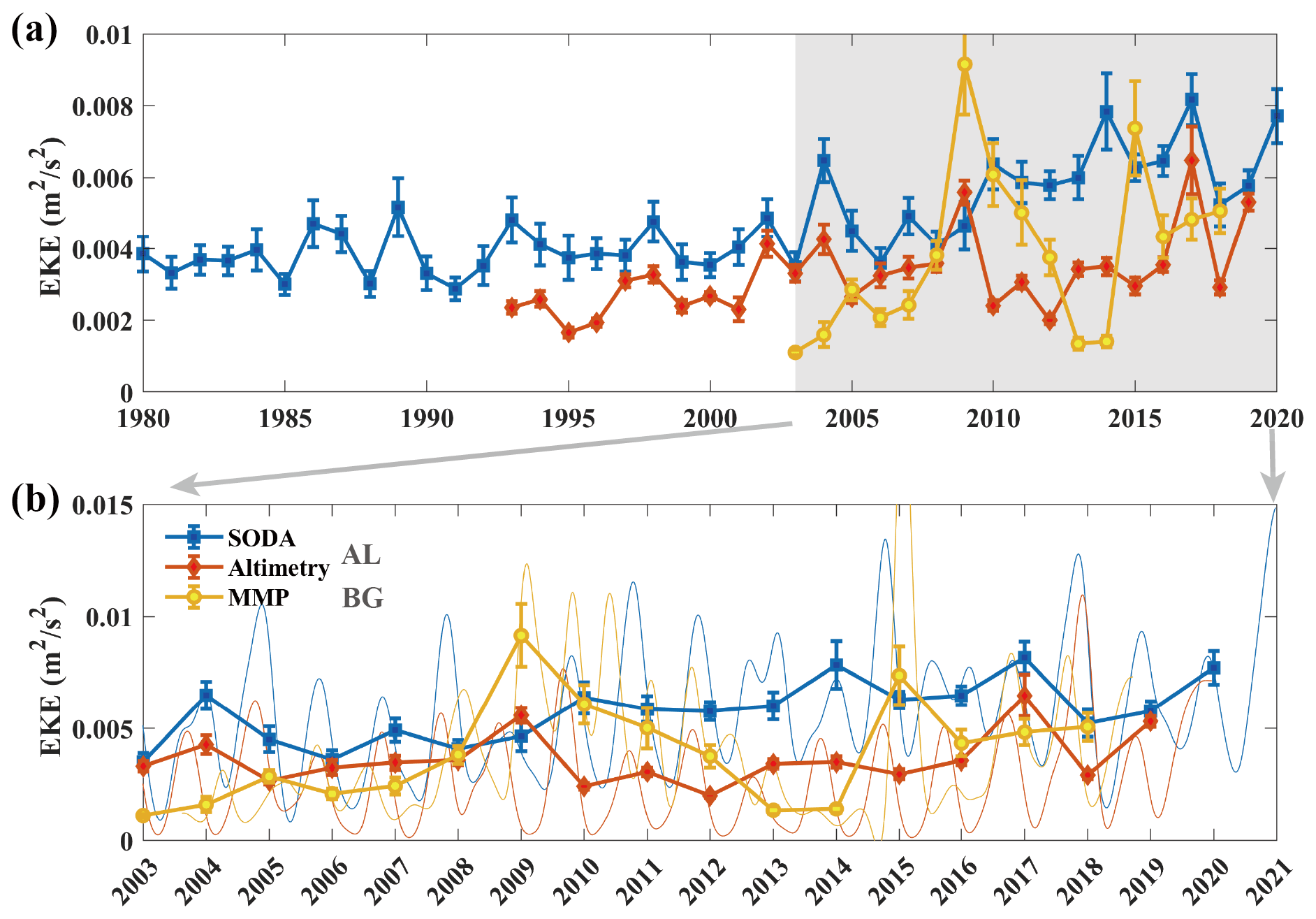
Figure 8 (a) Annual mean eddy kinetic energy (EKE) from MMP (2003–2018) averaged over 250 m in the BG region, as well as altimetry (1993–2019) and SODA (1980–2020) at the surface in the AL region. The error bars represent $\mathrm{1}/\mathrm{10}$ standard deviation in every year. (b) Annual mean EKE during 2003–2020 from the partial results of (a). The thin lines are the original time series smoothed by applying a 100 d low-pass filter.

5 Eddy modulation in the asymmetrical halocline

In the context of gyre variability and the most prominent sea ice losses in the BG region (Timmermans and Toole, 2023), extra wind energy input leads to more active eddies. Both surface and subsurface eddy activities are linked to gyre stability (Armitage et al., 2020; Manucharyan and Spall, 2016; Manucharyan et al., 2016). As discussed in Sects. 3 and 4, the halocline, as a measure of gyre stability, necessarily exhibits significant changes when the eddy number and strength are enhanced against this background. In particular, the variability in the halocline in the BG region demonstrates an apparent reduction in meridional asymmetry. How do eddies, as a key physical process, modulate the halocline in this phenomenon? In this section, we combine the variety of the eddy number and strength analysed in Sect. 4 with the varying asymmetry of the halocline to elucidate how eddy activities modulate in the halocline.

5.1 Relationship between geostrophic currents and EKE

The APE and geostrophic currents are both diagnostic variables of the halocline depth (Armitage et al., 2020). Eddies are generated by dissipating APE, and they gradually weaken the slope of isopycnals as well as geostrophic currents. Furthermore, the seasonality of eddy and geostrophic current fields is similar in the seas surrounding the Arctic (Armitage et al., 2017). EKE at the southwestern part of the basin with the confluence of reversed zonal geostrophic currents is the strongest (Fig. 9). The area with stronger (weaker) zonal currents has relatively weaker (stronger) EKE in the northern (southern) part of the Beaufort Sea slope (BSS) region.

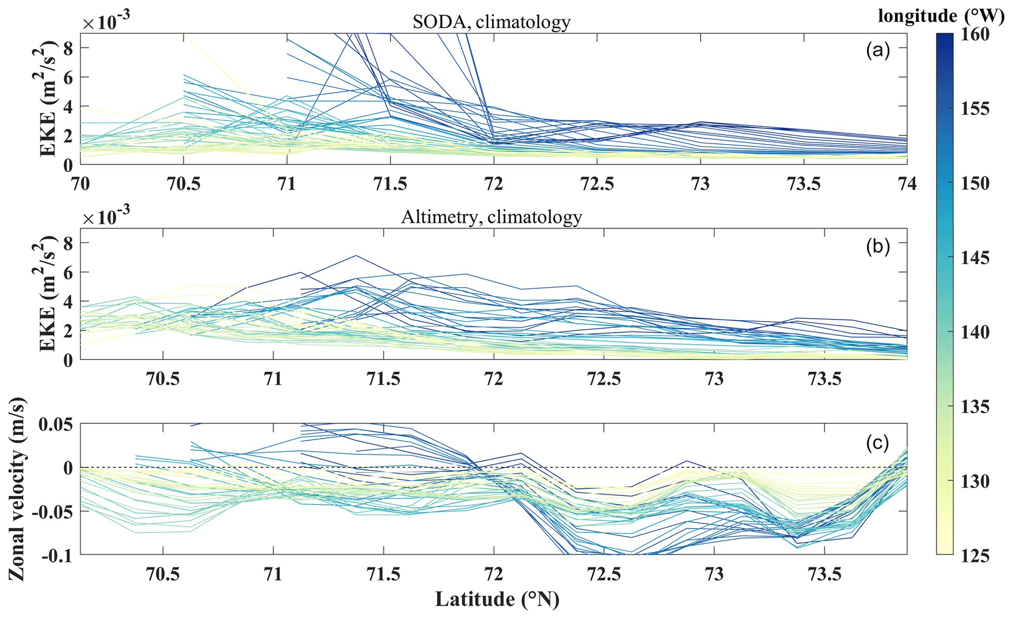
Figure 9 Climatological meridional eddy kinetic energy (EKE) from (a) SODA reanalysis (1980–2020) and (b) altimetry (1993–2019) in the Beaufort Sea slope (BSS) region. Panel (c) is the same as the upper and middle panels but for climatological zonal geostrophic velocity.

We compare the probability analysis results of EKE and geostrophic velocities averaged in the AL region based on the satellite altimetry in three periods (Fig. 10), which is estimated by the statistical frequency of the area mean time series in every period. The annual mean EKE was significantly intensified by 17 % (26 %) from period 1 to period 2 (from period 2 to period 3). Furthermore, its main values within the extent with a probability of 68.4 % were also enhanced. Although both velocities increased over the last two periods, the magnitudes of their increases were only 15 % and 7 %, which are much smaller than those of EKE. When the EKE in this region continued to increase sharply in the past, the velocity field increased more slowly. The increasing rate of velocity began to decrease, while EKE was still increasing rapidly, representing the fact that the difference between them has been magnified in recent years. For further clarification, we explore the relationship between these two variables. In addition, we find that these variabilities show a strong correlation over the area of interest (Fig. 10g). The correlation coefficients between EKE and local geostrophic velocities are mainly negative near the Alaskan coast and partial central basin, which is verified by their variation in the AL region. However, the major correlation coefficients passing the significance test level of 95 % remain highly positive between the 1000 and 3000 m isobaths along the southwestern margins of the basin, which is likely caused by the continuously enhanced EKE offshore that even emerges in the deep basin.

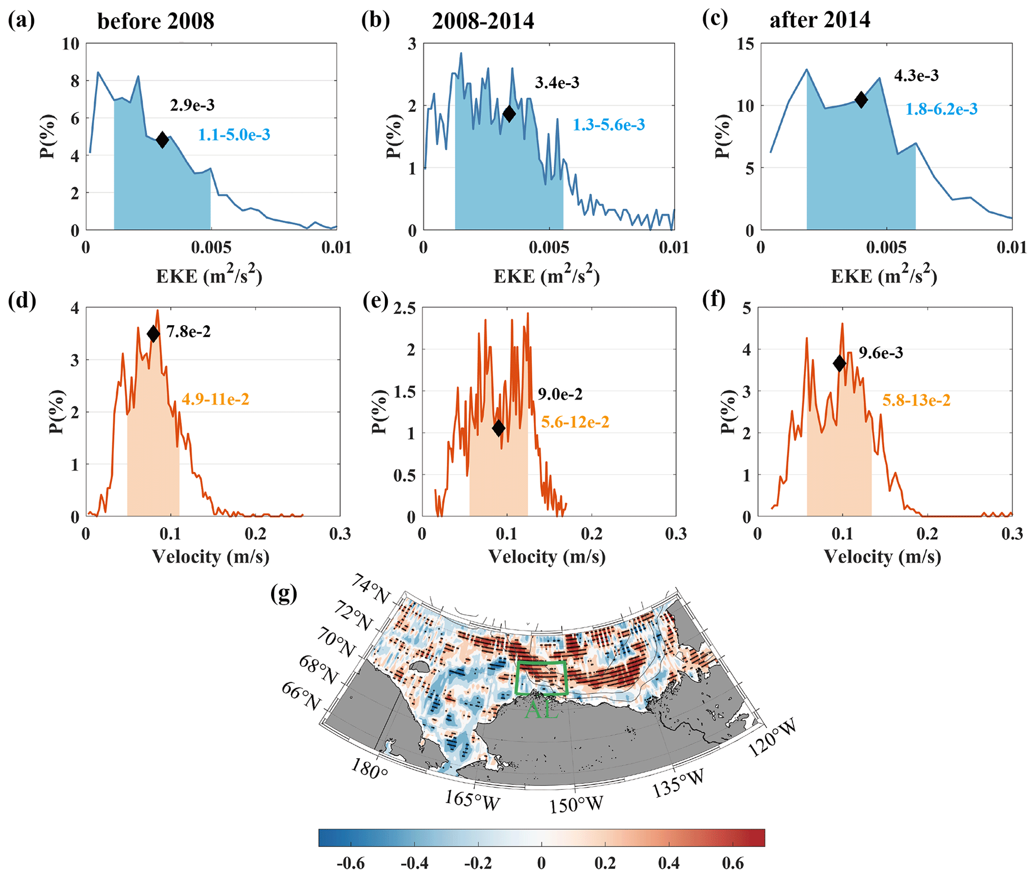
Figure 10 Probability of (a–c) eddy kinetic energy (EKE) and (d–e) geostrophic velocity in the Alaskan coast (AL) region during (a, d) 1993–2007, (b, e) 2008–2014, and (c, f) 2015–2019. The black diamonds represent the mean values in the three periods. The range of shading indicates the extent with a probability of 68.4 %. (g) A map of the correlation coefficients between the annual mean eddy kinetic energy (EKE) and local geostrophic velocities in 1993–2019. The black dots indicate all positions that passed a significance test (95 % confidence level).

5.2 Eddy lateral flux: a critical role in modulating the halocline

In recent years, after APE continuously decreased during 2010–2012 (Fig. 2a), EKE has remained at a relatively strong level compared with the mean value over the whole period (Fig. 8). In the meantime, the meridional asymmetry of the halocline geometry reduced, and the increasing rate of geostrophic currents slowed down. It is currently known that eddies can not only dissipate APE but also hinder freshwater accumulation. The halocline vertical structure has tended to be meridionally symmetrical in the BG region in recent years, which has been proven by observations and SODA reanalysis. The varying structure can be replicated well through schematic SODA reanalysis (Fig. 11a), although the results from SODA overestimate the depth of the halocline to a certain extent, with an error of 30–40 m near the central basin. The changes in the halocline structure on each side in the three periods obtained from SODA showed a strong consistency with the results from the CTD, which verified that the northern halocline of the central gyre was shallower and flatter than the southern part before 2008, and the halocline on each side along the meridional transect remained at a similar level after 2014.

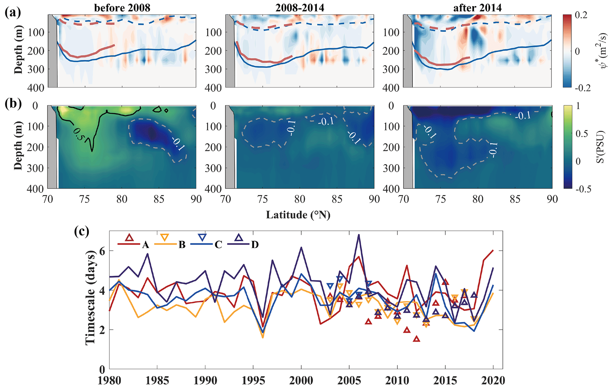
Figure 11 Transects of (a) the eddy stream function and (b) salinity anomaly relative to the whole term averaged in 2004–2007 (before 2008), 2008–2014, and 2015–2020/21 (after 2014), calculated from SODA simulated until 2020 and CTD observed until 2021. The dashed (solid) lines indicate the processed annual mean depth of the σ=25 (27.4) kg m⁻³ isopycnal surface representing the halocline top (base) from SODA (blue lines, selected data are from September to October, which is mostly consistent with the observed data for CTD deployment) and CTD (red lines) during three periods. (c) Annual mean time series of the Eady timescale calculated from SODA (solid lines) and MMP (triangles) at four moorings.

Aiming to explore the critical role that eddies play in the halocline, we analyse the eddy stream function evaluated by Eq. (5) over a long-term scale based on SODA. In the first period, when the Eady timescale was relatively larger over the long term (Fig. 11c), meaning stronger stability, the salinity anomalies in the mixed layer and the halocline layer were both positive (more than 0.5; Fig. 11b). Combined with the distribution pattern of the eddy stream function, the eddy thickness fluxes were generally positive at the surface, about 0.1 m² s⁻¹, representing the southward transport. However, in the halocline layer, relatively stronger eddy fluxes were mainly distributed at the southern and northern edges of the gyre, finally resulting in a southern halocline that is much steeper than the northern halocline at the same time. In the second period, when a transformation took place in the upper layer, the Eady timescale decreased, indicating enhanced baroclinic instability in the BG. There were low-salinity anomalies of about −0.2 in the halocline layer and eddy thickness fluxes of less than −0.1 m² s⁻¹. In the meantime, there was an overall deepening of the halocline depth. In the third period, there were significant low-salinity anomalies in the halocline within the BG region. In addition, the main spatial pattern of the eddy flux in this period was extremely similar to that in the former period but with obvious strengthening. In the mixed layer, the negative eddy thickness fluxes were about −0.2 m² s⁻¹. The eddy-induced transport replenished the freshwater at the northern edge. In the halocline layer, at approximately 71–79^∘ N surrounding the gyre centre, the convergence of eddy lateral fluxes was extremely strong. Eddy thickness fluxes can reach more than 0.1 m² s⁻¹ at the southern and northern edges, meaning that eddies transport water from either side into the stratified interior, which forms a centrally converging pattern. The freshwater redistribution induced by the eddy lateral flux, with the location of the central gyre being far from the south, contributed to the significantly flatter and inflated halocline surrounding the gyre centre, which led to reduced asymmetry. Some of the low-salinity water continued to spread northward, which coincided with the northward expansion and release of the freshwater from the gyre mentioned in a recent study (Bertosio et al., 2022).

6 Summary and discussion

In the past, the halocline deepened significantly in the deep basin and continental slopes (Kenigson et al., 2021; Zhong et al., 2019). In this study, our analyses of the halocline based on in situ hydrologic data, including moored observations and CTD, showed that the northern and southern depths of isopycnals around the central gyre have deepened to different degrees over almost the last 2 decades, which extends the analysis of asymmetrical stratification in the BG (Zhang et al., 2023). We found a reduction in meridional asymmetry in the halocline that has not been analysed in detail in previous studies. The halocline, around the central gyre, deepened by ∼ 40 and ∼ 70 m in the south and north, respectively, over the years 2003–2018. The meridional asymmetry of the halocline, with the halocline depth shallowing to the north, which initially induced a thinner halocline thickness in the north, was shifted to a final nearly symmetrical structure surrounding the central gyre.

However, eddy activity, a major factor affecting BG halocline dynamics, and its effects on asymmetrical structures have not been explored until now (e.g. Doddridge et al., 2019; Manucharyan and Spall, 2016). Our main objective is to explore how long-term variations in eddy activity affect the spatiotemporal variability in the asymmetrical halocline under the BG system. We investigated the spatiotemporal variability in eddies and EKE between the central gyre and continental slope, examining long-term eddy variability in particular, of which relevant research has been limited in the past. The eddy detection results agree with former studies (Zhao et al., 2014; Zhao and Timmermans, 2015). The majority of eddies are anticyclonic and cold-core eddies. With halocline depth varying, there are more active and stronger eddies in the final period than before. The highest-EKE region is close to the reversal currents with relatively weaker mean flows there. When EKE enhances along the Chukchi–Beaufort continental slope, it gradually develops towards the abyssal plain, which corresponds with its intensification in the interior gyre because of APE release in the final period, as seen with observations. Under increased eddy activity in the BG region, the halocline depth experienced a deepening and then a shallowing or stagnate phase in the BG region, and the increasing rate in geostrophic flows also slowed down. Surface and subsurface eddy activities jointly influenced oceanic stratification by inhibiting surface mean flows and promoting APE release above the halocline layer related to BG stabilisation (e.g. Armitage et al., 2020; Manucharyan and Spall, 2016).

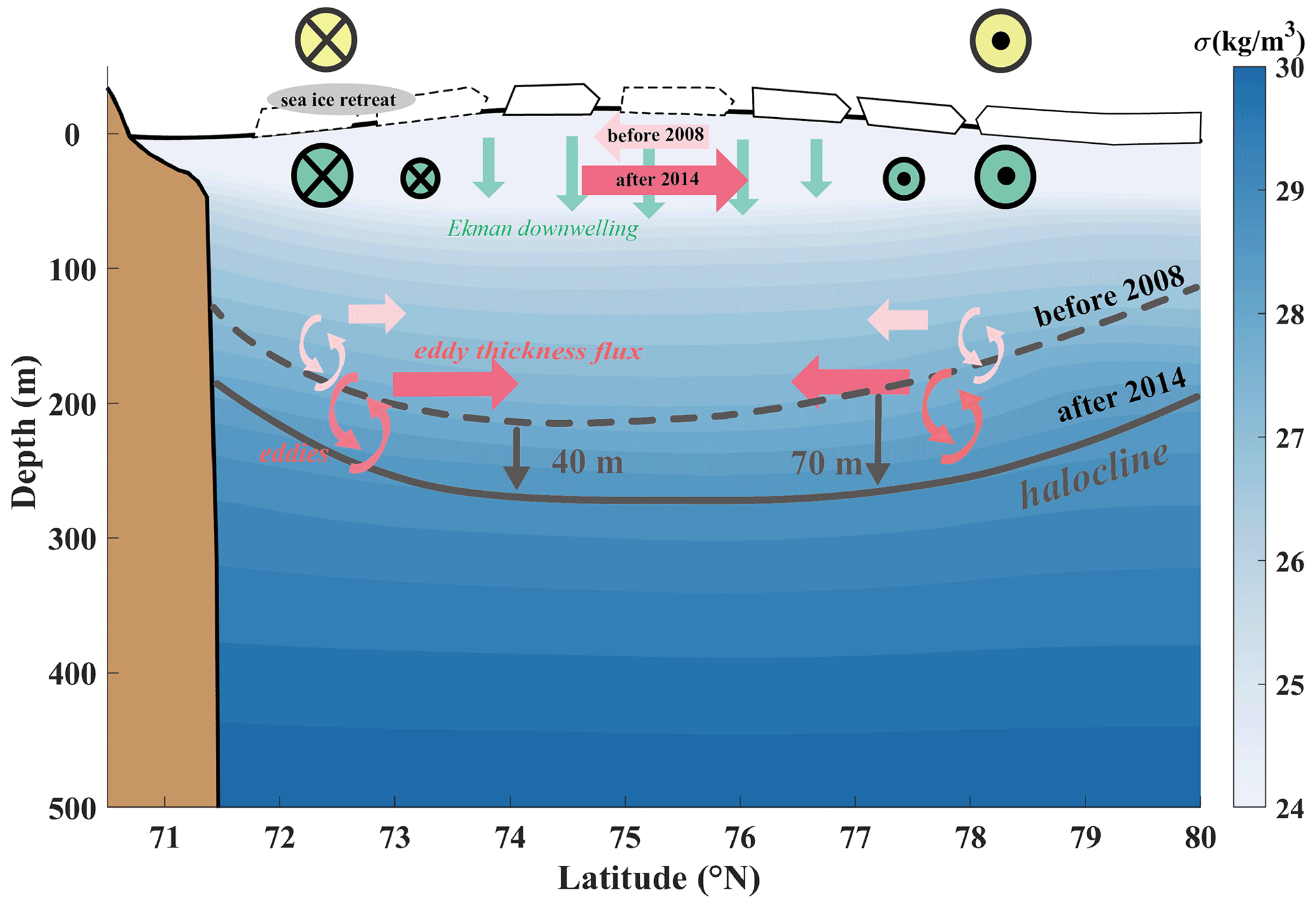
Figure 12 The schematic diagram under the BG system showing the transect of 150^∘ W, indicating the recent eddy modulation in the halocline. The shading is the climatological potential density from the 1990–2020 WOA climatology. The light (dark) pink arrows represent the eddy thickness flux before 2008 (after 2014).

Many studies support the hypothesis that the BG system is strongly affected by atmospheric dynamics that contribute to the deeper halocline in the interior gyre. The centre of the surface sea level dome and the wind-forced Ekman pumping area are also highly sensitive to wind patterns (Manucharyan and Spall, 2016; Regan et al., 2019; Timmermans and Toole, 2023). Eddy activity is also a major factor in the BG halocline. Overall, comparing the initial period with the final period (Fig. 12), the results revealed that the eddy lateral thickness fluxes, playing a critical role in modulating the halocline, have adjusted the vertical structure of the halocline by affecting the freshwater redistribution in the past few years. Currently, the meridional asymmetry of the BG halocline is distinctly diminished due to strengthened modulation of the eddy lateral fluxes. A series of processes through eddies promoted the surface northward transport and freshwater confluence in the halocline at depths from two sides, which adjusted the deformation of the halocline structure.

To date, previous studies have hypothesised that the accumulation of freshwater driven by Ekman pumping is balanced by the effect of mesoscale eddies for stabilising the circulation (e.g. Davis et al., 2014; Manucharyan and Spall, 2016), not probing too much into the spatial difference in the halocline structure. Our research supports the reduction in the meridional asymmetry in the BG halocline and related eddy modulation as a role in the reduction, providing a perspective for understanding the relationship between long-term changes in the stratification structure and eddy field. We expect our study to expand the knowledge of large-scale circulation and mesoscale processes against the background of rapid changes in the Arctic. It is still necessary to use high-resolution simulations combined with observations across the gyre to obtain a comprehensive understanding of interior variations between different physical processes in order to promote scientific development in BG dynamics.