the Creative Commons Attribution 4.0 License.
the Creative Commons Attribution 4.0 License.
 | 22 Feb 2023
Observation-based estimates of volume, heat, and freshwater exchanges between the subpolar North Atlantic interior, its boundary currents, and the atmosphere
Sam C. Jones
Neil J. Fraser
Stuart A. Cunningham
Alan D. Fox
Mark E. Inall
The Atlantic Meridional Overturning Circulation (AMOC) transports heat and salt between the tropical Atlantic and Arctic oceans. The interior of the North Atlantic subpolar gyre (SPG) is responsible for the much of the water mass transformation in the AMOC, and the export of this water to intensified boundary currents is crucial for projecting air–sea interaction onto the strength of the AMOC. However, the magnitude and location of exchange between the SPG and the boundary remains unclear. We present a novel climatology of the SPG boundary using quality-controlled CTD (conductivity–temperature–depth) and Argo hydrography, defining the SPG interior as the oceanic region bounded by 47∘ N and the 1000 m isobath. From this hydrography we find geostrophic flow out of the SPG around much of the boundary with minimal seasonality. The horizontal density gradient is reversed around western Greenland, where the geostrophic flow is into the SPG. Surface Ekman forcing drives net flow out of the SPG in all seasons with pronounced seasonality, varying between 2.45 ± 0.73 Sv in the summer and 7.70 ± 2.90 Sv in the winter. We estimate heat advected into the SPG to be between 0.14 ± 0.05 PW in the winter and 0.23 ± 0.05 PW in the spring, and freshwater advected out of the SPG to be between 0.07 ± 0.02 Sv in the summer and 0.15 ± 0.02 Sv in the autumn. These estimates approximately balance the surface heat and freshwater fluxes over the SPG domain. Overturning in the SPG varies seasonally, with a minimum of 6.20 ± 1.40 Sv in the autumn and a maximum of 10.17 ± 1.91 Sv in the spring, with surface Ekman the most likely mediator of this variability. The density of maximum overturning is at 27.30 kg m−3, with a second, smaller maximum at 27.54 kg m−3. Upper waters (σ0<27.30 kg m−3) are transformed in the interior then exported as either intermediate water (27.30–27.54 kg m−3) in the North Atlantic Current (NAC) or as dense water (σ0>27.54 kg m−3) exiting to the south. Our results support the present consensus that the formation and pre-conditioning of Subpolar Mode Water in the north-eastern Atlantic is a key determinant of AMOC strength.
- Article
(12006 KB) - Full-text XML
-
Supplement
(1196 KB) - BibTeX
- EndNote


The Atlantic Meridional Overturning Circulation (AMOC) is the zonally integrated system of currents transporting heat and salt between the South Atlantic and the Arctic Mediterranean. It is a key component of the global thermohaline circulation, transporting approximately 25 % of the global ocean–atmosphere heat transport. Meridional heat transport associated with the AMOC is 1.2 PW across 26∘ N (RAPID, Smeed et al., 2018), diminishing to 0.51 PW at 58∘ N (OSNAP, Li et al., 2021b) and 0.27 PW by the Greenland–Scotland Ridge (Chafik and Rossby, 2019). The subpolar North Atlantic (SPNA) plays a large role in regulating the climate system by connecting surface and deep layers, such that variability in these regions can imprint on global averages and mediate the rate of climate change (Chen and Tung, 2014; IPCC, 2021).
The SPNA features a cyclonic system of currents collectively termed the subpolar gyre (SPG), transporting warm, salty water northwards on its eastern side and transitioning into a cool, fresh southward flow on its western side. The strongest currents in the SPG are located around the periphery due mainly to meridional density gradients and topographic intensification in the east (Huthnance et al., 2022; Marsh, 2017) and western intensification in the west (Munk, 1950; Stommel, 1957; Sverdrup, 1947). The Gulf Stream is the primary input of water to the SPG from the south. As the Gulf Stream crosses the Atlantic from west to east, a portion transitions into the North Atlantic Current (NAC); about 55 % of NAC transport is thought to circulate in the SPG, while the remainder is diverted poleward over the Greenland–Scotland Ridge (Berx et al., 2013; Hansen et al., 2015; Østerhus et al., 2019). Return flow into the SPG from the Arctic Ocean and Nordic Seas mainly occurs in deep overflows over the Greenland–Scotland Ridge (Dickson et al., 2008; Johnson et al., 2017; Østerhus et al., 2008) and in the surface outflow of Polar Water in the East Greenland Current (De Steur et al., 2017).
The generally accepted view of the AMOC functioning in the SPNA has been that wintertime buoyancy loss in the Labrador Sea drives deep convection and that this convection was the principal direct linkage of the upper and lower limbs of the overturning (e.g. Rhein et al., 2011), though some contemporary studies have argued that the contribution of the Labrador Sea to the AMOC was more minor (e.g. Pickart and Spall, 2007). Observations from the OSNAP array have provided strong evidence that the mean and variability in the SPG AMOC is driven by buoyancy exchanges in the ocean basins north of OSNAP-East (Kostov et al., 2021; Li and Lozier, 2018; Li et al., 2021a; Lozier et al., 2019; Petit et al., 2020, 2021). Processes north of the Greenland–Scotland Ridge (GSR) also contribute significantly to the supply of dense water to the lower limb of the AMOC (Chafik and Rossby, 2019; Petit et al., 2021; Tsubouchi et al., 2021; Zhang and Thomas, 2021).
A reconciliation of these views is a new appreciation that most of the density anomalies evident in the Labrador Sea are generated by buoyancy exchanges in the east and imported to the Labrador Sea. Therefore, while the Labrador Sea density anomalies are an ultimate indicator of SPG AMOC functioning, they are not the source drivers (Li et al., 2021a; Menary et al., 2020). Instead, the transformation of the NAC to Subpolar Mode Water (SPMW, Brambilla and Talley, 2008; Brambilla et al., 2008) appears to play a key role in pre-conditioning for overturning at higher densities (Petit et al., 2021). A remaining challenge for tracking the AMOC is therefore understanding the location, nature, and hierarchy of processes connecting SPMW with the eventual export of dense waters in the lower limb.
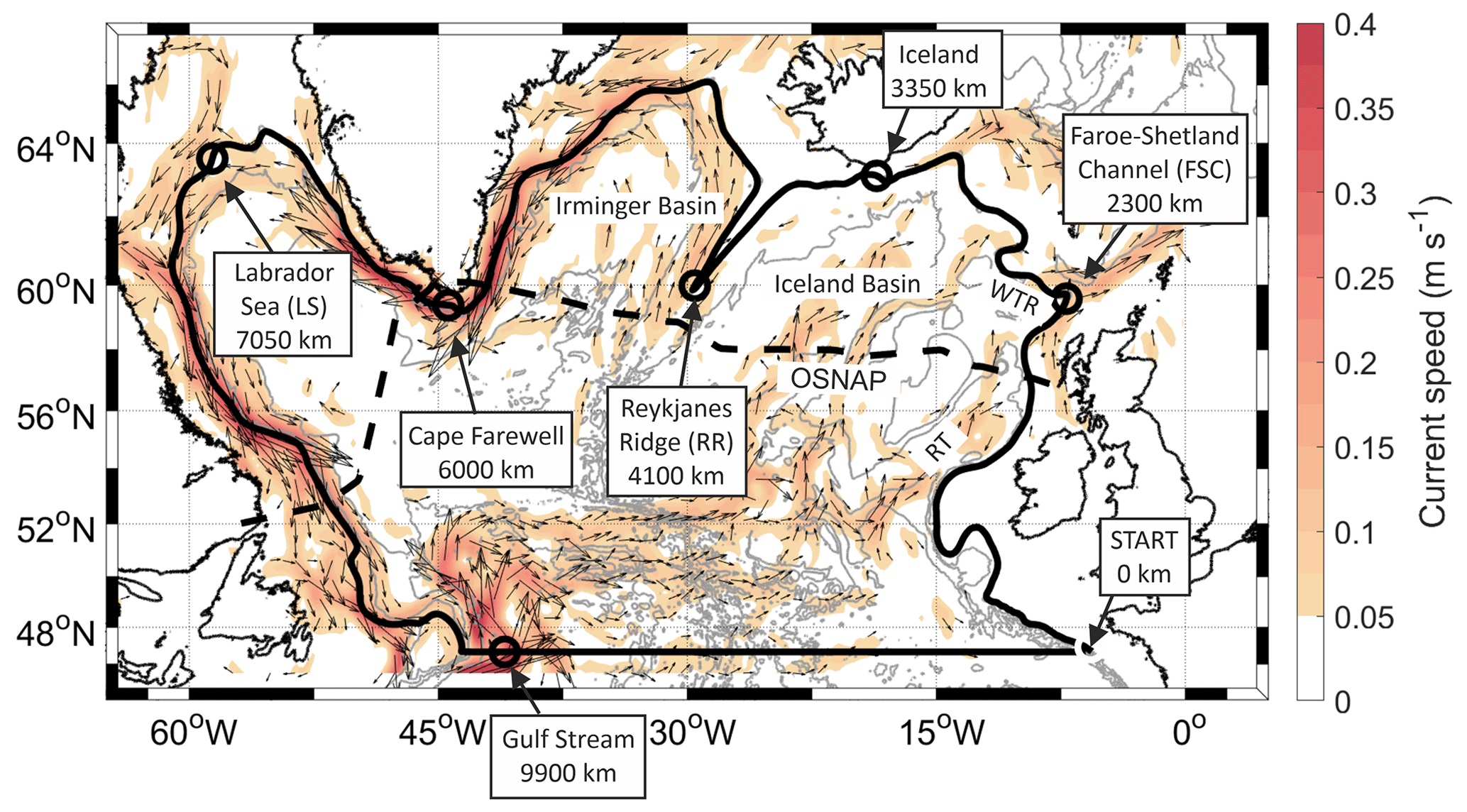
Figure 1Smoothed 1000 m bathymetry contour (solid black line) closed by transect across 47∘ N. Key locations around contour are labelled; these are used throughout this study. The dashed black line shows the OSNAP line. OSNAP-West denotes the portion of the line west of Greenland, and OSNAP-East denotes the portion of the line east of Greenland. RT is the Rockall Trough, and WTR is the Wyville Thomson Ridge. Mean magnitude and direction of surface currents (2000–2020) derived from AVISO data are shown by coloured contours and quiver arrows. Isobaths are overlaid at 1000 m increments. Bathymetry contours from GEBCO bathymetry (http://www.gebco.net/, last access: 15 June 2020). GEBCO stands for the General Bathymetry Chart of the Oceans.
One way of further refining our understanding of AMOC is to distinguish processes taking place in the SPG interior from those external to the SPG (mainly in the SPG boundary and north of the GSR, e.g. Desbruyères et al., 2020; Petit et al., 2021; Tsubouchi et al., 2021). This can be achieved by examining the interface (Liu et al., 2022; Spall, 2008) between the SPG interior where much of the buoyancy forcing takes place (De Jong et al., 2018; Josey et al., 2019) and the narrow, swift boundary currents that rapidly transmit this information around the SPG and enable connections with other basins (Fig. 1). For example, interior–boundary exchange can be influenced by changes in water mass properties in the boundary currents (Williams et al., 2015), wind forcing (Huthnance et al., 2022), and interaction between boundary currents and steep topography driving diapycnal mixing (Brüggemann and Katsman, 2019; Le Bras et al., 2020; Liu et al., 2022; Spall and Pickart, 2000).
To evaluate the importance of these boundary processes to the SPG AMOC, we calculate a budget for the exchange of water between the SPG interior and boundary or shelf regions and through a zonal transatlantic section at 47∘ N (Fig. 1). We construct a new temperature–salinity (TS) climatology along the 1000 m depth contour of the SPG and closing at 47∘ N (12 000 km path, Fig. 1) covering the Argo era (2000 onwards).
The 1000 m isobath was selected for numerous reasons. Firstly, the 1000 m contour encircles the key features of the SPG, including the Rockall, Iceland, Irminger, and Labrador basins, partitioning basin interior processes from shelf sea processes. Secondly, at 47∘ N the simulated maximum overturning in depth space is roughly 1000 m depth (Hirschi et al., 2020), so this choice allows us to approximately distinguish upper and lower limb processes. Thirdly, Argo trajectories allow us to estimate currents at 1000 m depth that we later incorporate into our analysis.
We quantify regionally and in density space where the volume transports into and out of the SPG interior occur. We then validate and extend our analysis using the VIKING20X model (Biastoch et al., 2021; Fox et al., 2022), which, when combined with our new climatology, provides novel insights into the functioning of the AMOC in the SPG. We present the overturning, heat and freshwater fluxes associated with the observed water properties and transports. Finally, we investigate which processes determine how volume continuity is maintained in the SPG and summarise it in a schematic (Fig. 12).
Here we describe the datasets and methods used for the core analyses in the study. Information on other datasets used is provided in Supplement Sect. S2.
2.1 World Ocean Database (WOD18) profile data
We construct our TS climatology along a narrow strip defined by the 1000 m isobath around the basin of the SPG. CTD (conductivity–temperature–depth) and Argo profile data from post-2000 (Argo era) were downloaded from the WOD on 3 September 2019 (Boyer et al., 2018a). The isobath was smoothed using a 100 km along-contour bracket to remove undesired complexity in the contour and profiles of conservative temperature (T) shown in Fig. 2. We required data coverage between surface and 1000 m so profiles with poor vertical resolution (<50 observations), and those sampling only part of the water column, were excluded. Further quality control steps were performed and are detailed in Sect. S1.
2.2 Gridding of profile data
Profiles were first separated into four seasons: winter (JFM), spring (AMJ), summer (JAS), and autumn (OND). They were gridded vertically in 20 dbar (1 dbar is equal to 10 kPa) pressure bins and then horizontally. For the horizontal gridding we used cells spaced at regular 150 km intervals and employed a variable search radius centred on each cell. The along-slope property gradients were weaker and decorrelation scales larger (e.g. Davis, 1998) than those in the across-slope direction, so we considered a larger grid size and search radius in the along-slope direction to be appropriate. For a given grid cell, an initial search radius of 150 km was used, and the number of profiles found in this radius of a cell was evaluated. If 75 raw profiles were not found, this search radius was incrementally expanded up to a maximum of 300 km. Thus, most profiles are used in more than one grid cell. Most grid cells are populated using the minimum search radius (150 km), but it was necessary to expand the search radius up to the maximum 300 km to achieve good coverage in 5 % of cells during the summer, rising to 22 % during the autumn. No centre-weighting process was attempted. Profiles were averaged on pressure levels to create the gridded product of T and S. A schematic of the gridding workflow is provided in Sect. S1.
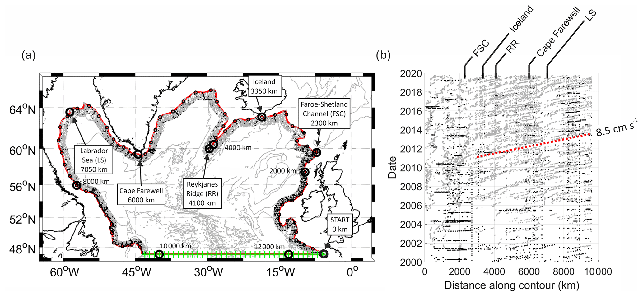
Figure 2(a) Location of profiles contributing to the basin perimeter data product. Black points show CTD profiles, while grey points show Argo profiles. The 1000 m bathymetry contour is shown in red. The profiles extend up to 75 km offshore from the 1000 m contour. Small black circles on boundary contour show grid locations of boundary data product, while green crosses show grid locations of EN4 zonal section at 47∘ N. Bathymetry contours from GEBCO bathymetry (http://www.gebco.net/, last access: 15 June 2020). GEBCO stands for General Bathymetry Chart of the Oceans. (b) Distribution of profiles contributing to the boundary dataset plotted over time. Black points show CTD profiles, while grey points show Argo profiles. The dashed red line shows the average Argo float speed of 8.5 cm s−1 around the boundary. Key locations around boundary are labelled as follows: Faroe–Shetland Channel (FSC), the southernmost point of Iceland, Reykjanes Ridge (RR, southern tip), Cape Farewell, and the Labrador Sea (LS).
2.3 EN4 data at 47∘ N
We use temperature and salinity data from the Met Office EN4 product (Good et al., 2013) for the zonal section to close the boundary at a latitude of 47∘ N. We considered this to be the most appropriate source of data for the zonal transect: first, while our boundary dataset benefitted from an “along-boundary” gridding methodology, the zonal transect is aligned to EN4's grid, so the benefits of independently gridding the profile data are largely negated. Second, EN4's climatology provides coverage deeper than 2000 m in the North Atlantic, a region where observational data are sparse due to the depth limit of most Argo floats.
We found excellent agreement between gridded profiles and EN4 grid cells in <2000 m waters and no unusual horizontal gradient in properties (which could translate into an anomalous geostrophic transport) between the end of the boundary dataset and the beginning of the EN4 transect. The location of WOD profile data and EN4 grid cells is shown in Fig. 2. We found that below 1000 m, geostrophic velocities calculated from EN4 data overestimated the strength of the Gulf Stream and underestimated the Deep Western Boundary Current and other southward flows across 47∘ N due to data coverage limitations in the abyssal ocean. In Sect. 2.4.5 we discuss this weakness and the steps taken to limit its impact on the results.
2.4 Computing transports and fluxes
2.4.1 Geostrophic velocities
We first compute the geostrophic shear between each gridded station, and between the final station and the first to complete the loop. Note that when integrating to the same depth around the loop, the net transport between the interior and exterior of the SPG is constrained to be near-zero because there is no net change in dynamic height around the closed circuit. A small residual transport remains because of variations in the Coriolis parameter f as the latitude of the stations changes around the boundary (the “beta effect”).
When computing overturning transport and heat and freshwater fluxes in Sect. 3.4 and 3.5, we require a measure of transports to the seabed so that volume is conserved on completion of the boundary loop. Geostrophic velocities across the >1000 m depth of the 47∘ N transect result in a net gain in volume by the SPG interior, so we enforce the conservation of volume using a small negative reference velocity applied to this region. The EN4 dataset is known to poorly resolve the Deep Western Boundary Current in this region (Fraser and Cunningham, 2021), which explains some of this imbalance. The implementation of this reference velocity and its impact on computed values for fluxes and overturning are discussed in Sect. 2.4.5.
Dynamic height at each profile is computed relative to the surface and referenced to the gridded absolute dynamic topography (ADT) derived from satellite altimetry (Eq. 1). We consider the use of satellite sea surface height (SSH)-derived velocities to be a robust reference method for our application given the large spatial scales and the long temporal averages associated with the study. The gridded ADT data were temporally averaged over the same periods as the profile data coverage (2000–2019, split into four seasons), and interpolated values were extracted at the station locations. They were then smoothed using a five-point running average to mimic the smoothing inherent in the hydrographic gridding process.
Here, Φbc is the dynamic height relative to the sea surface, calculated as the integral of the specific volume anomaly from the gridded pressure to the surface, η is the satellite-derived ADT, and g is acceleration due to gravity. The time-mean geostrophic velocity vgeo assigned to locations mid-way between hydrography stations is computed from
where x is the (anticlockwise) distance along the 1000 m contour.
2.4.2 Geostrophic transports
Transports for each grid cell (Qgrid cell) were computed by integrating Eq. (2) over the cross sectional area between each station and between adjacent pressure levels (the 20 dbar pressure intervals are taken to approximate 20 m):
The vertically integrated transport between 0 and 1000 m can then be computed by summing the transports of cells at each station. Further, the accumulated transport around the basin can be obtained using a horizontal integral. We estimate statistical uncertainties based on the variability inherent in the datasets contributing to the study. This is accomplished by repeating the analysis multiple times with the gridded TS profiles randomly perturbed. The perturbation of each gridded value is scaled by the standard deviation of profile data contributing to that grid cell, thus giving an indication of the sensitivity of the conclusions to the scatter of “raw” profiles. For the EN4 transect, the uncertainty is supplied with the gridded variables, and we use this to scale the perturbations. The satellite altimetry has a large standard deviation on day or month timescales. As our analysis spans 2 decades, we considered it appropriate to first calculate annual means of ADT, then compute the standard deviation of these annual means for the uncertainty estimate. The ADT accounts for about 60 % of the uncertainty for the heat and freshwater fluxes and about 30 % of the uncertainty for the overturning results. The analysis was repeated 100 times with the boundary climatology, altimetry, and surface Ekman transports (Sect. 2.4.3). The standard deviation of the resultant values forms the upper and lower bounds supplied with our results. Measurement errors are substantially smaller than the standard deviation of observations. Calibrated CTDs are typically accurate to ± 0.001 ∘C and ±0.002 psu, and delayed-mode calibrated Argo floats are accurate to ±0.005 ∘C and ± 0.01 psu. Errors in SSH in the gridded ADT product are typically around 1–2 cm in the North Atlantic but are up to 7 cm in the Gulf Stream. As these measurement errors are generally not systematic, the long averaging periods in our analysis mean that they make a negligible contribution to the total uncertainties.
At some locations the boundary contour is by necessity oriented along the boundary current, which implies the along-contour isopycnal slope is small compared to the across-contour slope in these regions. As such, the across-contour geostrophic transports for these grid cells will be small residuals of the along-contour transports. We would expect these regions of the boundary product to be particularly sensitive to temporal or spatial biases in the sampling. However, as we accumulate the geostrophic transports around the basin, the distances over which the along-contour isopycnal slope is evaluated are large relative to the across-contour slope. Therefore, while along-contour flows may contaminate the signal for individual grid cells, they should have minimal impact on the accumulated transports. The uncertainties arising from our perturbation experiments provides some insight into the sensitivity of the results to local sampling errors (e.g. Fig. 5).
We investigated the gridded ANDRO dataset as a complementary source of 1000 m velocities but found that the small across-slope component of flow described above, coupled with the proximity of the continental slope, made the product unsuitable for our investigation.
2.4.3 Surface Ekman transports
Wind stress data were obtained from the ECMWF ERA5 reanalysis product (Hersbach et al., 2020). The wind stress component tangent to the boundary contour was used to calculate the Ekman transport across the boundary at geostrophic velocity locations (cell mid-points). These were then averaged to compose seasonal climatologies. Uncertainties associated with the surface Ekman transports were taken as the standard deviation of annual means of the transports. For the flux and overturning calculations, the Ekman transports are added to velocities in the top 20 m cell. They therefore act on the corresponding top cells of the gridded temperature and salinity.
2.4.4 Model-derived transports in VIKING20X
We recreate the boundary transect in VIKING20X to support the observational analysis and help diagnose the transports and fluxes that may not be resolved by geostrophic or surface Ekman calculations. Output of the VIKING20X-JRA55-short model hindcast (Biastoch et al., 2021) is used to compute transports into the SPG. VIKING20X is a 0.05∘ ice and ocean model of the Atlantic Ocean (33.5∘ S to ∼65∘ N) nested within a 0.25∘ global ice and ocean model. The run used here is driven from 1980–2019 using JRA55-do atmospheric forcing and runoff (Tsujino et al., 2018). In the vertical, VIKING20X uses 46 geopotential z levels with layer thicknesses from 6 m at the surface gradually increasing to ∼250 m in the deepest layers. Bottom topography is represented by partially filled cells, allowing for an improved representation of the bathymetry (Barnier et al., 2009). In the SPNA, VIKING20X has horizontal resolution of 3–4 km. Hindcasts of the past 50–60 years in this eddy-rich configuration show that it realistically simulates the large-scale horizontal circulation, the distribution of the mesoscale, overflow and convective processes, and the representation of regional current systems in the North and South Atlantic (see Biastoch et al., 2021, for full details).
To preserve the volume conservation in VIKING20X, rather than mimicking the observational data sampling the transport calculations are performed across a section following horizontal grid cell boundaries (T-grid boundaries in the VIKING20X ocean Arakawa C-grid). North of 47∘ N this section is constructed to be the shallowest line with all adjacent cells deeper than 1000 m, the volume is closed across 47∘ N. Total model transports, model geostrophic transports (referenced to model sea surface height), and model surface Ekman transports are calculated.
The stepped model topography results in two potential approaches for estimating geostrophic transports. The first stops strictly at 1000 m but leaves a small gap beneath over complex bathymetry. This approach obeys the beta constraint on geostrophic flow, so is most comparable to the observations but some “leakage” below 1000 m on the boundary remains. The other approach extends to the bed around the boundary. This means that all across-boundary flow is captured, but the beta constraint on total geostrophic transport is slightly relaxed as there is now an undulating bed with along-section pressure differences. When comparing observations to VIKING20X (Sect. 3.3) we primarily use transports derived using the strict 1000 m cut-off. However, when estimating the gyre volume budget (Sect. 4.4) we compute transports to the seabed around the boundary as this enforces a strict separation of flows across the 47∘ N transect.
To diagnose ageostrophic near-bed flow associated with the modelled boundary current, an estimate of model bottom Ekman transport QEB (per unit section length) into the SPG is made:
from model parameters Cd=0.001 and eb=0.0025 m2 s−2. Cd is the bottom drag coefficient, and eb the bottom turbulent kinetic energy loss due to tides, internal waves breaking, and other short-timescale currents. u is along-section velocity, v is velocity perpendicular to the section, and f is the Coriolis parameter.
2.4.5 Heat and freshwater fluxes
For this analysis the gridded temperature and salinity are interpolated onto the “mid-point” geostrophic velocity stations and σ0 recalculated. The computation of fluxes requires a mass-balanced velocity field, and this necessitates computing transports down to the seabed rather than for the top 1000 m only. Whilst we have confidence that geostrophic and surface Ekman transports together capture the main flow features of the upper ocean, as previously stated we consider that geostrophic shear using the EN4 TS fields does not adequately resolve several features of the deep flow across 47∘ N. Computing cumulative geostrophic and surface Ekman transports for the full depth results in residuals averaging +20 Sv into the SPG, mainly because the Gulf Stream does not diminish with depth but also due to an underestimation of the Deep Western Boundary Current and an absence of southern flow in the deep water masses across 47∘ N. We therefore perform a two-stage adjustment to the sub-1000 m velocities to first linearly reduce the Gulf Stream with depth, then add a seasonally varying reference velocity that when added to the 47∘ N section (integrated between 1000 m and seabed) balances the water volume entering and leaving the SPG. This is between −0.0002 and −0.0018 cm s−1 depending on season. Details of this adjustment are provided in Sect. S5.
Heat and freshwater fluxes across the boundary were calculated as follows. Heat flux (Qθ) across each grid cell is defined as follows:
Where ρ is the nominal potential density of seawater, Cp is the specific heat of seawater, vtotal(x,z) is the sum of the geostrophic (Eq. 1) and Ekman velocities (Sect. 3.2.2) perpendicular to the section, θ(x,z) is the conservative temperature, and (the reference temperature) is the mean temperature for the full-depth SPG interior (4.03 ∘C). Following Lozier et al. (2019), we use a value of 4.1×10⁶ J m−3 K−1 for ρCp.
Freshwater flux (Qf) is defined as follows:
where S(x,z) is the absolute salinity of a grid cell, and (the reference salinity) is the mean salinity for the full-depth SPG interior (35.14 g kg−1). As before, the convention for Qθ and Qf is positive into the SPG.
We estimate the average surface freshwater and heat fluxes for 2000–2019 using ERA5 monthly means (Hersbach et al., 2020). For freshwater we compute evaporation and precipitation for each grid cell, then integrate over the total surface area enclosed by the 1000 m contour and 47∘ N (4.6×10⁶ km2) using an area-weighted mean. We calculate downward surface heat flux as the sum of sensible, latent, shortwave, and longwave heat fluxes. Surface flux errors are estimated as the standard error of the annually averaged time series for the summed components following Li et al. (2021a).
2.4.6 Eddy kinetic energy and boundary topography
Eddy kinetic energy (EKE) was calculated from satellite ADT for the period of study using
where and are the high-frequency components (150 d high-pass filtered) of the unsmoothed surface geostrophic velocity components along the SPG boundary contour. The overbar denotes seasonal averaging to form climatologies.
Seabed slope angle was calculated from 30 arcsec GEBCO bathymetry on the native grid (GEBCO compilation group, 2019) then interpolated onto ∼1 km horizontal resolution rendition of the 1000 m depth contour (derived from the same GEBCO data set). A 480-point moving mean was applied along the contour. Slope is a scale-dependent quantity: at the visual map scale a 480-point running mean does not equate to a 480 km straight line moving average since at the 1 km scale the 1000 m contour is highly irregular.
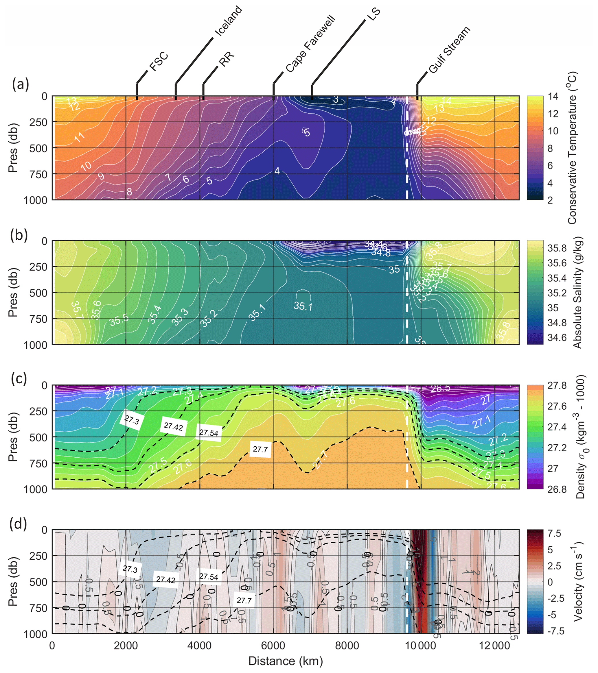
Figure 3Gridded boundary product plotted by distance along the 1000 m contour travelling anticlockwise around the basin (annual means shown): (a) conservative temperature (∘C), (b) absolute salinity (g kg−1), (c) density (σ0, kg m−3), and (d) geostrophic velocities across the boundary perpendicular to the 1000 m depth contour (cm s−1, positive into the interior, negative out of the interior, colour map intervals of 0.25 cm s−1 with selected contours shown). Density contours relevant to overturning processes (Fig. 9) are shown by dashed black lines in (c) and (d). The transition to the 47∘ N section and from gridded CTD to EN4 climatology data is delineated by the dashed white line. Key locations around the boundary are labelled: Faroe–Shetland Channel (FSC), southernmost point of Iceland, Reykjanes Ridge (RR, southern tip), Cape Farewell, the Labrador Sea (LS), and the Gulf Stream.
3.1 Hydrography
The cyclonic evolution of water properties around the closed SPG boundary is shown in Fig. 3, and a full-depth section across 47∘ N is shown in Fig. 4. These figures depict the annual average water properties; seasonal anomalies are supplied in Sect. S3.
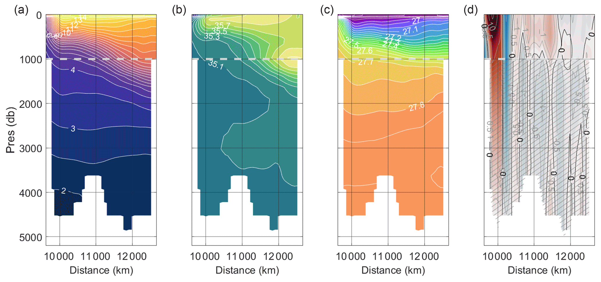
Figure 4Zonal (47∘ N) section constructed from EN4 data and shown to full depth for (a) conservative temperature (∘C), (b) absolute salinity (g kg−1), (c) density (σ0, kg m−3), and (d) geostrophic velocities into the SPG perpendicular to contour (cm s−1). Annual means are shown. The sub-1000 m region in (d) delineated by cross-hatching is subject to a correction velocity (see Sect. S5 for details). The 1000 m vertical threshold for transport calculations is delineated by the dashed white line.
In general, the density at a given depth level increases with progress along the 1000 m isobath. By the thermal wind relation, the geostrophic shear is therefore typically negative (i.e. increasing density in a cyclonic direction driving export across the boundary out from the interior). Between the boundary start near the Bay of Biscay and the Faroe–Shetland Channel (FSC) the water column is thermally stratified and this controls the density distribution (salinity changes only gradually with depth). Between 1000 and 2000 km (European Shelf), the along-section density gradient at a fixed depth is positive at points shallower than 750 dbar and is negative deeper than 750 dbar. This is consistent with the expected density evolution of the adjacent slope current in this region (Huthnance et al., 2022). The horizontal density gradient increases at the entrance to the FSC. Between here and Iceland, a persistent negative geostrophic flow, strongest near the surface, is associated with a thermally driven positive density gradient. Between Iceland and Cape Farewell, further cooling, freshening, and densification occurs throughout the water column. Geostrophic flow out of the SPG is largely shallower than 500 dbar, and into the interior it is below 500 dbar. This implies an export of light surface waters from the SPG, their external conversion to denser classes, and their re-import at depth. We do not see the very cold (<3 ∘C) and dense (>27.8 kg m−3) waters suggestive of the Faroe Bank Channel overflow or the Denmark Strait Overflow (DSO) at their expected locations along the boundary (approximately 3000 and 5000 km, respectively, Johnson et al., 2017; Mastropole et al., 2017). We return to this point and discuss the significance of the overflows later in the paper.
Cape Farewell marks the beginning of a pronounced change to the water column structure. West of Cape Farewell (i.e. along western Greenland) there are positive geostrophic flows associated with the introduction of a cold, fresh, low-density surface layer shallower than 250 dbar. This change in water properties may be associated with offshore fluxes of freshwater from the Greenland shelf into the Labrador Sea interior near Cape Farewell (Lin et al., 2018) and farther north where the West Greenland Current (WGC) becomes unstable (Fratantoni, 2001; Prater, 2002). The positive geostrophic flow may also partly result from the WGC moving into deeper water and thus crossing our perimeter contour in this region. There is also a negative horizontal density gradient below 250 dbar, but this is driven by an increase in temperature with progress around the gyre. In the north-western Labrador Sea, the trend towards increasing density is resumed, this time driven by further cooling below 250 dbar.
Geostrophic flow in the north-western Labrador Sea is into the SPG and is greatest at depth. The influence of the cold Labrador Current in the surface layers extends along the Newfoundland and Labrador shelf edge as far as 47∘ N. Horizontal density gradients are very weak over this region, consequently geostrophic flow is near-homogeneous with depth. The boundary tracks the northern rim of the Flemish Cap before crossing the North Atlantic at 47∘ N. The Labrador Current is bisected here as it exits the SPG. The Gulf Stream is clearly visible on the western side of the 47∘ N transect as a narrow region featuring rapid warming and salinification driving a steep negative horizontal density gradient. This is associated with a region of very strong barotropic flow into the interior and strong flow out of the interior immediately adjacent. Thermal wind results in a reduction of current strength with depth. East of the Gulf Stream system, the zonal transect is largely characterised by positive geostrophic flow northward and weakening with depth.
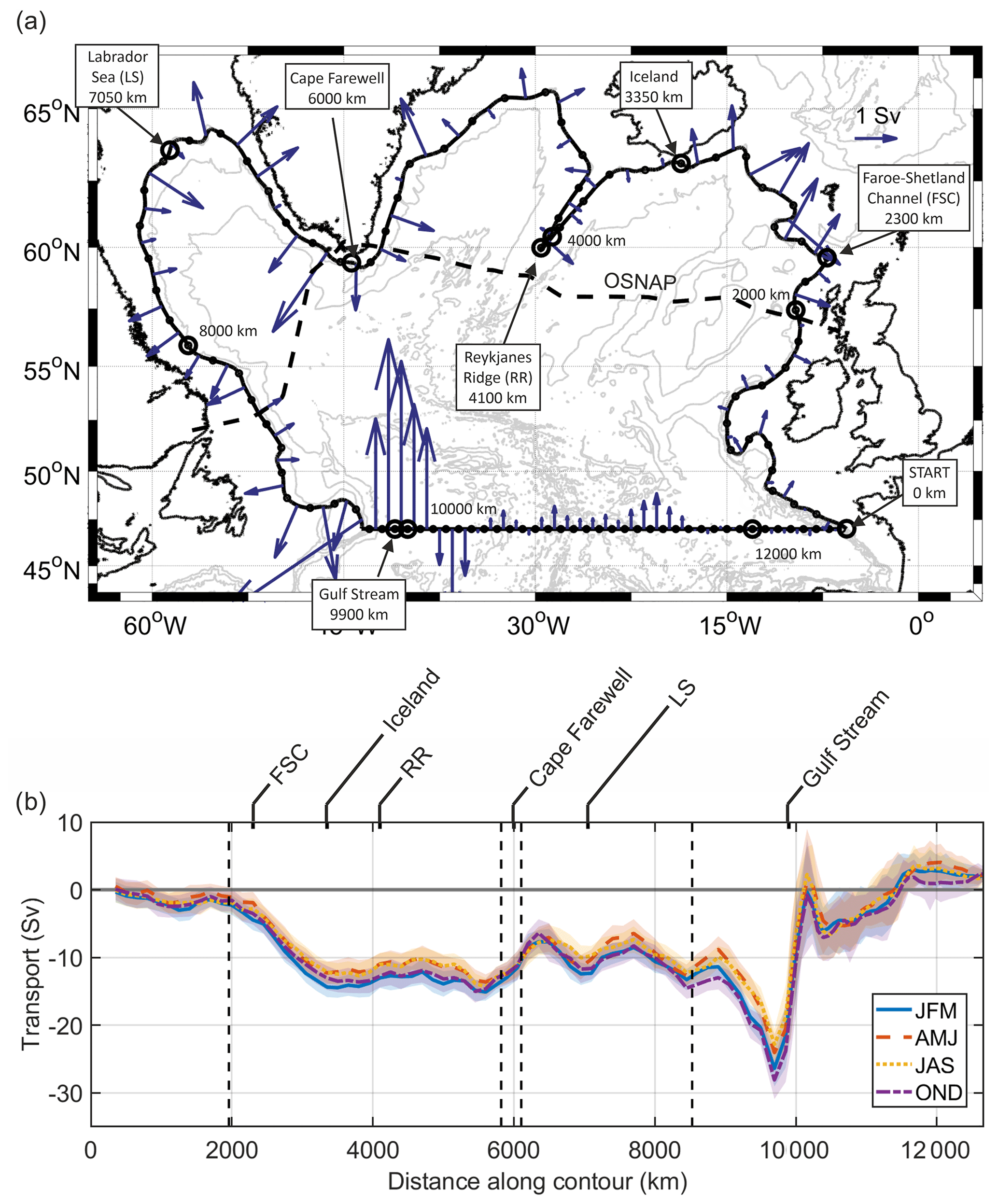
Figure 5Geostrophic transport perpendicular to contour; positive values denote transport into the SPG. (a) Depth-integrated volume transport between 0 and 1000 m for each grid cell (time series and annual mean). Quiver arrows show the magnitude of transport across grid cell and are constrained to be perpendicular to the section. Horizontal bins are 150 km apart around the 1000 m contour and 1∘ across 47∘ N. Bathymetry contours from are General Bathymetry Chart of the Oceans (GEBCO, http://www.gebco.net/, last access: 15 June 2020). (b) Cumulative volume transport around basin for each season. Key locations around boundary labelled as in Fig. 3, and vertical dashed lines denote OSNAP crossings.
3.2 Transports perpendicular to boundary
3.2.1 Geostrophic transports above 1000 m
The depth-integrated geostrophic transport across the boundary (Fig. 5a) is broadly out of the SPG in the FSC and to the east of Iceland and to the west of the Gulf Stream. Inflow is dominated by northward flow across 47∘ N (above 1000 m) mostly in the Gulf Stream (+20 to 30 Sv) but also across the width of the Atlantic. However, within this there are striking regional patterns of inflow and outflow and regions where there is only limited flow across the boundary. Along the European continent there is outflow south of Ireland and then inflow to the north, perhaps a suggestion of cyclonic circulation over the Porcupine Bank at shallower depths. North of Ireland some outflow is evident, suggesting transport onto the Malin and Hebridean shelf (Jones et al., 2018, 2020; Porter et al., 2018). Between Scotland and Iceland, −10 to −12 Sv of outflow marks the exit of the NAC towards the Iceland–Scotland Ridge. This is larger than estimates of outflow over the ridge itself (−7.1 Sv, Østerhus et al., 2019), indicating that some of this exported water contributes to the boundary current and does not exit the basin in this region. Around the Reykjanes Ridge the pattern of flow is consistent with net westward cross-ridge flow quantified by Petit et al. (2018). Northward flow of Atlantic Water in the upper layers through Denmark Strait (−1 to 2 Sv) is consistent with observations of the Denmark Strait inflow (−0.9 Sv, Jonsson and Valdimarsson, 2012; Semper et al., 2022). Flow in the vicinity of Cape Farewell is notable for the large transports into the SPG associated with the East Greenland Current (EGC) and its retroflection (5.1 Sv, Holliday et al., 2007), while outflow in the north-eastern Labrador Sea is the result of a portion of the WGC exiting the SPG towards Davis Strait. Approximately the same volume re-enters the SPG along northern Labrador as a portion of the Labrador Current, which flows parallel to the boundary down the Labrador and Newfoundland shelf and shelf edge (Lavender et al., 2000). Note that it is not possible to exclude the boundary currents entirely from the SPG by choosing a deeper boundary reference contour. A large portion of flow in the WGC and Labrador Current occurs offshore of the 2000 m isobath, and the choice of a deeper contour has other drawbacks, as discussed in Sect. 1. At 53∘ N (the western OSNAP crossing) for example, the core of the Labrador Current is inshore of the 1000 m isobath, but the southward flow extends 75–100 km offshore of the 1000 m isobath (e.g. Zantopp et al., 2017). This portion of the boundary current must exit the domain to the south and west. From about 7800 km to west of the Gulf Stream, sustained outflow results in a net export of 12 Sv, of which about half is onto the shelf (Figs. 1, 5a). The outflow through the Flemish Pass and around the Flemish Cap accounts for the remainder (Petrie and Buckley, 1996).
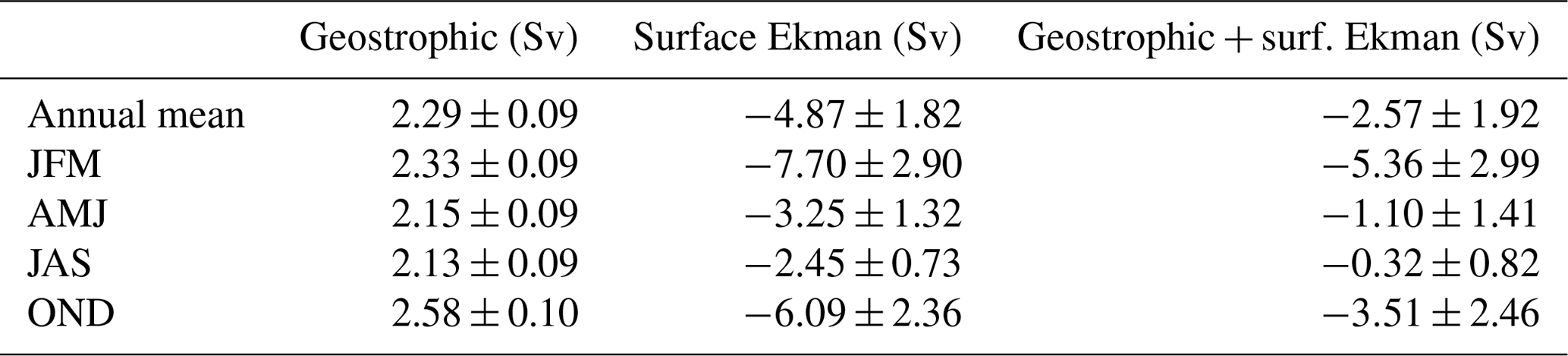
Along 47∘ N, east of the Gulf Stream inflow, there is a narrower region of recirculating outflow and then a weak inflow across most of the section to the east. The net cumulative transports into and out of the SPG return to near zero on completion of the circuit, with a small positive residual in all seasons (+2.13 to +2.58 Sv) due to the beta effect. Cumulative geostrophic transports above 1000 m are shown in Table 1.
Seasonal transport variations are relatively small (Fig. 5b). Between the FSC and the western Irminger Sea (5500 km) autumn and winter transports out of the SPG are 1–2 Sv greater than spring and summer before converging at Cape Farewell. Similarly, along the Labrador Seaboard autumn and winter transports out of the SPG tend to be greater than those in spring and summer but converge when crossing the Gulf Stream.

Figure 6Surface Ekman transport perpendicular to contour, into the SPG positive. (a) volume transport between 0 and 1000 m for each grid cell, coloured by season. Quiver arrows show magnitude of transport across grid cell, and are constrained to be perpendicular to the section. Horizontal bins are 150 km apart around the 1000 m contour, and 1∘ across 47∘ N. Bathymetry contours are from General Bathymetry Chart of the Oceans (GEBCO; http://www.gebco.net/, last access: 15 June 2020). (b) Cumulative volume transport around the basin for each season. Key locations around the boundary are labelled as in Fig. 3, and vertical dashed lines denote OSNAP crossings.
3.2.2 Surface Ekman transport perpendicular to boundary
Due to the prevalent cyclonic weather systems over the SPNA, surface Ekman transport is generally directed out of the SPG, with winter exhibiting the largest transports and summer the weakest (Fig. 6). South-westerly winds in the north-eastern Atlantic result in net transports out of the SPG onto the continental shelf west of the British Isles. Between Scotland and Iceland there is little surface Ekman transport across the boundary, due mainly to the prevailing surface Ekman transport being roughly parallel to the boundary contour rather than lower wind speed (e.g. Laurila et al., 2021). Conversely, very high transports out of the SPG off south-eastern Greenland are due both to energetic storm systems and to the boundary contour being approximately perpendicular to prevailing surface Ekman flow. There is strong seasonality off south-eastern Greenland, with cumulative transports varying from −0.5 Sv in the summer to −2 Sv in the winter. Off south-western Greenland there is net inflow into the SPG (except in summer). This is the only location that sees seasonal sign reversal (+1 Sv in winter to −0.2 Sv in summer). While the Labrador Sea gains volume off south-western Greenland during the winter, between Cape Farewell and the OSNAP-West crossing at 8500 km there is a net loss of −1.8 Sv in the winter compared to −0.1 Sv in the summer, resulting in a large seasonal signal from this region. Between the western Labrador Sea and the Gulf Stream, surface Ekman transports are almost exclusively out of the SPG. This trend continues across the 47∘ N section, with a further strengthening of the net seasonal signal due to weak spring and summer negative transports contrasting with strong autumn and winter transports. Net surface Ekman transports out of the SPG range from −2.45 Sv in the summer to −7.70 Sv in the winter (Table 1).
The surface Ekman transports, when summed with the geostrophic transports, contribute a marked seasonal component to the net cumulative transport across the boundary. In winter there is a −5.36 Sv residual transport out of the SPG, whereas in the summer the residual reduces to −0.32 Sv (Table 1), with the seasonal range driven almost entirely by the surface Ekman component.
3.2.3 Bottom Ekman transport
Bottom Ekman transport is an essential dynamical feature of cyclonic ocean boundary (slope) currents (Huthnance et al., 2020) and a significant transport mechanism from slope regions to adjacent ocean interior (Huthnance et al., 2022). Typical slope boundary current velocities range from a few to several tens of centimetres per second. We make an approximate observation-based estimate of the bottom Ekman transport using the 1000 m drift characteristics of Argo floats contributing to the boundary dataset (Fig. 2b). The advection of floats around the SPG boundary is visible as diagonal stripes, particularly after 3000 km. We investigated the gridded ANDRO dataset as a potential source of boundary current velocities but found that the proximity of the continental shelf made the interpolation scheme unsuitable in some areas. Instead, using the temporal and spatial displacements of floats between successive profiles, we compute the average along-slope speed around the SPG boundary to be 8.5 cm s−1 (dashed red line, Fig. 2b).
We estimate the bottom Ekman transport into the SPG following theoretical arguments by Souza et al. (2001) and Simpson and McCandliss (2013). However, as there is a quadratic dependence of bottom stress on current speed, simply taking the mean along-slope speed of the floats will result in an underestimate of the bottom Ekman transport. To address this concern, we use the approach suggested by Zhai et al. (2012), in which a transport correction factor, β, is computed given the magnitude of the variability as a fraction of the mean, α. Here we take the variability to be the standard deviation of float speeds (7.5 cm s−1) so α has a value of 0.88. The bottom Ekman transport QEB is then
where β can be approximated as (Zhai et al., 2012), kb is a bottom friction coefficient (taken as 0.0025 following Simpson and McCandliss, 2013), is the mean along-slope speed, and f is the local Coriolis parameter. As f varies around the boundary, we compute QEB for each grid cell on the boundary and integrate horizontally. This results in a total transport into the SPG of 2.5 Sv.
Given the large uncertainties associated with the observation-based bottom Ekman estimates we exclude this process in the transports contributing to the overturning and flux totals; however, it is relevant to the discussion of the SPG volumetric budget. The potential contribution of bottom Ekman transport and other near-bed processes to the SPG volume budget is discussed in Sect. 4.4.
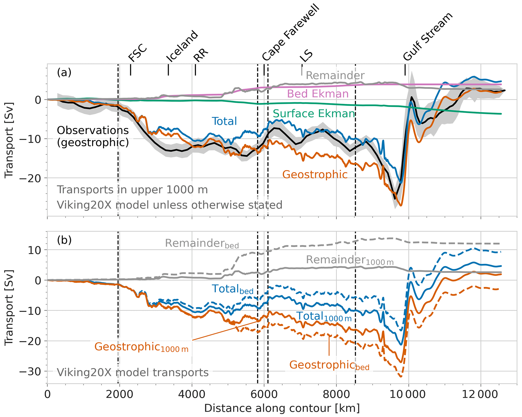
Figure 7(a) Comparison between observed cumulative geostrophic volume transport into the SPG (annual mean) and transport components above 1000 m in VIKING20X. Key locations around the boundary are labelled as in Fig. 3, and vertical dashed lines denote OSNAP crossings. he remainder is calculated as the total transport minus the geostrophic, surface Ekman, and bed Ekman transport components. (b) Comparison between transports into the SPG in VIKING20X using a strict 1000 m cutoff and integrating to the bed along the 1000 m contour (but still integrated to 1000 m across 47∘ N). The difference is due to the stepped model topography and associated inability to follow the 1000 m bathymetry precisely.
3.3 Transports perpendicular to the boundary in VIKING20X
The 20-year mean geostrophic volume transports into the SPG calculated from the VIKING20X model hydrography show broad agreement with the observation-based geostrophic transports at large spatial scales (Fig. 7a). Both show outward transport of 25–30 Sv around the 1000 m contour, balanced by inward transport in the surface 1000 m across 47∘ N, with a total net inflow of 2–3 Sv around the full perimeter. The geostrophic transport of the Gulf Stream above 1000 m is about 25 Sv in both the model and observations. Between the FSC and Iceland, 12 Sv is exported out of the SPG in the observed transports, while 9 Sv is exported in the model. The modelled and observed transports then converge and exhibit little difference between the RR and Cape Farewell.
At smaller spatial scales there are dissimilarities between model and observational geostrophic flows. VIKING20X has steady outflow through FSC, and east and west of Iceland, contrasting with the observations which show outflow focussed in the FSC and Iceland–Faroe Ridge (2000–3000 km), though the total transport accumulated between the FSC and the OSNAP crossing east of Cape Farewell is the same in each case. There is a contrast in behaviour around the Labrador Sea. VIKING20X shows 5 Sv of spatially uniform outflow from the interior between Cape Farewell and the western end of OSNAP, whilst the observations show alternating regions of inflow and outflow round the Labrador Sea. In particular, the model has no inflow to match observations at the northern half of western Greenland. There are also different patterns of inflow across 47∘ N, with the model showing stronger inflow in the region east of the main Gulf Stream core but west of the Mid-Atlantic Ridge (10 300–11 000 km).
There are many possible reasons for these differences and a detailed examination is beyond the scope of the current work. The Labrador Sea boundary is a region of very steep topography, complex interactions, and poorly understood freshwater influence. Model TS and density structure in this region may be unrealistic (see Biastoch et al., 2021). The model section and the observational climatology are constructed quite differently along the 1000 m section: the model hydrography is sampled along a single line closely following the 1000 m contour, while the observations involve spatial averages over large (75 km × 150 km) areas offshore of this contour. Observed geostrophic velocities are referenced to satellite-derived ADT at the surface, these are at coarser resolution than the dynamically consistent modelled sea surface heights used to reference the VIKING20X geostrophic velocity calculation.
In calculating transports from the observation-based climatology we consider the contribution from geostrophy in the top 1000 m and surface wind forcing. The SPG boundary features regions of steep topography, strong boundary currents, deep overflows, and enhanced eddy activity, and it is therefore unclear how much of the total cross-boundary flow we are capturing. We can use the model results to look at details of the missing transports. Figure 7a shows two candidate processes: the first is bottom Ekman layer frictional flow, while the second is primarily driven by non-linear and viscous processes. In Fig. 7b we examine the possible missing transports due to flows beneath the base of our 1000 m contour and the bed (due to the observed climatology being on average offset from the continental slope; see Fig. 2). In VIKING20X this is achieved by integrating to the bed along the 1000 m contour, as opposed to using a strict 1000 m cutoff. The difference arises due to the stepped model topography and associated inability to follow the 1000 m bathymetry precisely.
The results show that over most of the boundary the across-boundary flows are dominated by geostrophic flows (solid and dashed orange lines, respectively, Fig. 7a and b). The major exceptions are the deep overflow regions of the Denmark Strait (around 5000–5500 km), and, to a smaller extent, the Faroe Bank Channel overflow at around 3000 km. While these unobserved processes dominate the cross-boundary transports at two locations, they account for the majority of the cross-boundary transport when integrated round the whole boundary above 1000 m (grey and dashed grey lines, Fig. 7a and b). We discuss this further in Sect. 4.5.
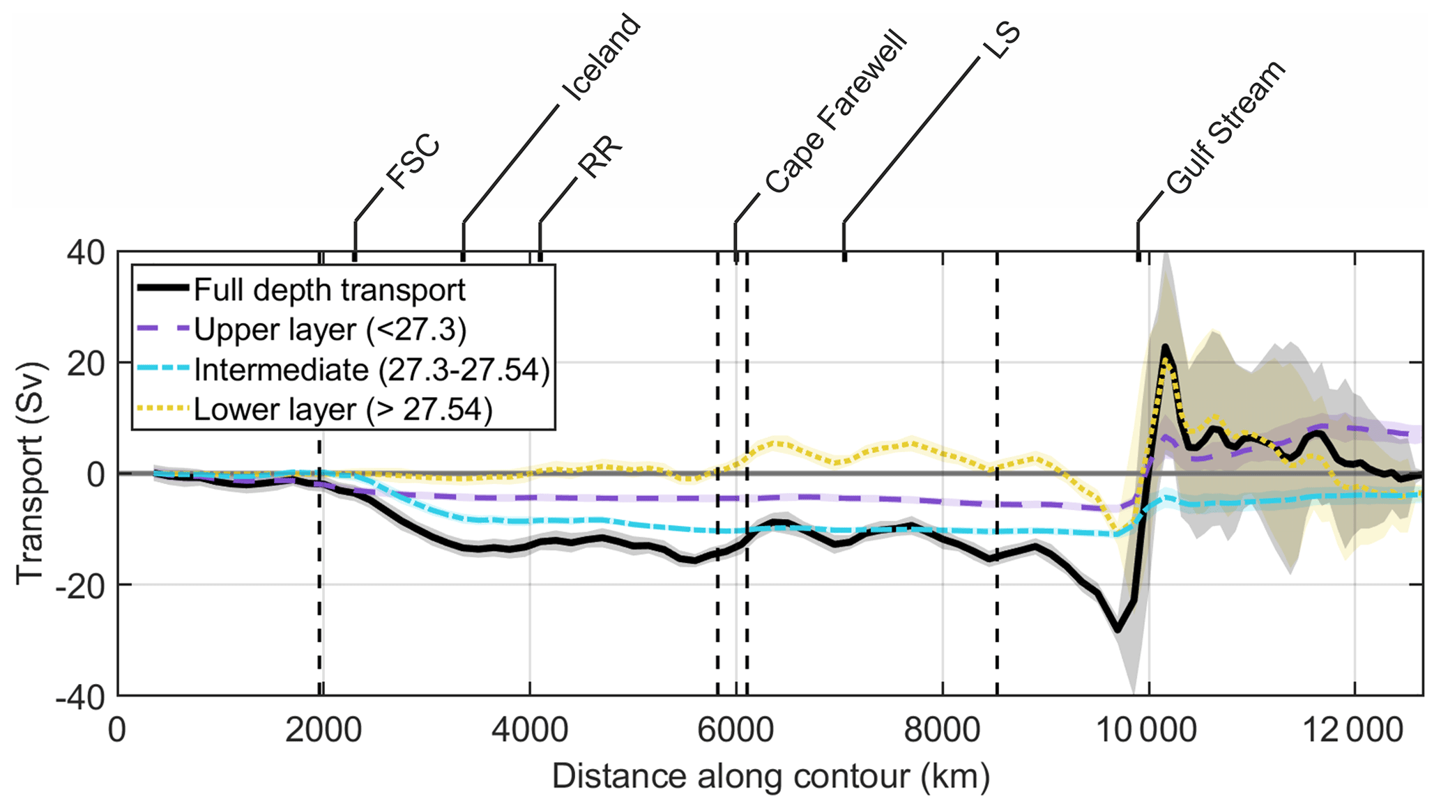
Figure 8Cumulative volume transport into the SPG interior (geostrophic plus surface Ekman) between the surface and the seabed. Adjustment velocity is applied below 1000 m to conserve volume. Transport in the upper, lower, and intermediate layers is also shown; these are defined in Sect. 3.4. Key locations around the boundary are labelled as in Fig. 3, and vertical dashed lines denote OSNAP crossings.
3.4 Overturning in the subpolar gyre
Here we compute the density–space overturning circulation in the SPG using the sum of the observed geostrophic and surface Ekman fluxes. Note that in the context of this study, the term “overturning” describes the transformation occurring within a closed contour, in contrast to studies computing overturning north of an open section such as OSNAP. For this analysis it is necessary to integrate to the seabed across the 47∘ N transect so we apply a reference velocity below 1000 m on the 47∘ N transect to enforce the conservation of volume (Sect. S5). The full-depth transports are shown in Fig. 8. As the adjustment is applied to waters below 1000 m, it almost exclusively impacts lower limb flows and is below the main features of the overturning stream function (Fig. 9).
The full-depth transports in Fig. 8 are divided into upper, intermediate, and lower layers based on density thresholds established using inflection points in the overturning stream function (Fig. 9). These density thresholds are also overlaid on the density and geostrophic velocity sections depicted in Fig. 3c and d. The upper layer has a net gain of 7.36 ± 1.48 Sv, while the intermediate and lower layers have a net loss of −3.85 Sv and −3.53 Sv, respectively. The upper layer loses volume around the SPG from the Bay of Biscay to the Gulf Stream. This loss of ∼2.5 Sv occurs around 2000 km and is associated with surface cooling and exchange with the European shelf. Approximately 0.5 Sv (20 %) of the loss is due to air–sea heat exchange, and the remaining 2 Sv (80 %) is advected out of the SPG by geostrophic and Ekman flows.
West of the FSC, the water column is sufficiently dense that the upper layer makes little further contribution to the total transport. The intermediate layer accounts for almost all of the NAC transport out of the interior across the Iceland–Scotland Ridge. As the boundary contour advances around the Irminger Basin (4100–6000 km), the lower layer becomes the dominant contributor to the total transport. The lower layer accounts for most of the inflow in the vicinity of Cape Farewell and the subsequent regions of inflow and outflow in the Labrador Sea and along northern Labrador. The export of water west of the Gulf Stream is also almost entirely in the lower layer. The Gulf Stream drives transport into the interior in all layers, though the contribution is largest in the lower layer.
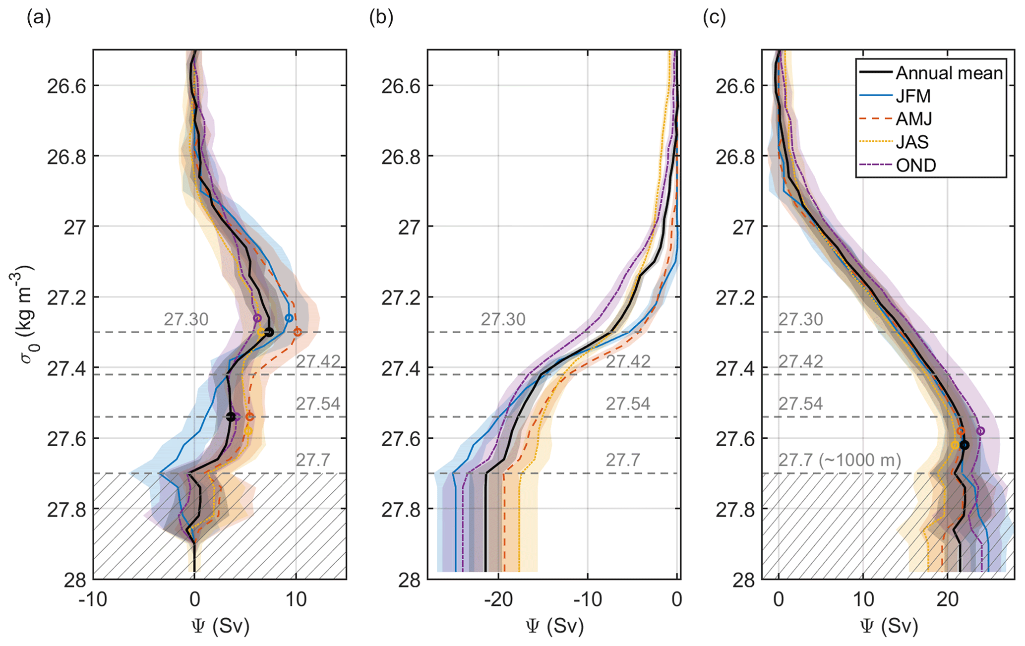
Figure 9(a) Overturning stream function ψ for the full SPG boundary in density space between surface and seabed using corrected velocities for sub-1000 m currents. Density of maximum overturning and that of secondary peak (where applicable) are highlighted by circles. Densities of mean inflection points marked by horizontal dashed grey lines; these are overlaid on Fig. 3c and d. The hatched area denotes the approximate density space impacted by the sub-1000 m correction velocities (see Sect. S5 for details). Panel (b) is the same as (a) but for boundary contour (0–9500 km) only, while (c) is the same but for the 47∘ N transect (9500–12 700 km) only.
The overturning stream function, ψ, is a measure of the amount of water transformed to higher densities in each density class. We compute the overturning in density space following Lozier et al. (2019):
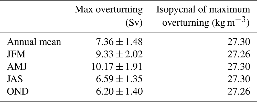
This is shown for each season and for the annual mean in Fig. 9a. The main peak in the overturning stream function occurs at densities between 27.26 and 27.30 kg m−3 (Fig. 9, Table 2), with maximum overturning varying between 6.20 Sv in summer and 10.17 Sv in spring. A smaller secondary peak exists at higher density classes (27.54 to 27.58 kg m−3) in all seasons but winter, with maximum overturning values of 3.59 to 5.50 Sv.
Table 2Overturning strength and its location in density space by season.
We investigate this signal by deconstructing the mean (Fig. 9b and c). Figure 9b and c show the transports accumulated over density space for the 1000 m isobath and 47∘ N transect components of our section, respectively. About 8 Sv is exported across the 1000 m contour in the density range 27.3 to 27.42 kg m−3 (Fig. 9b). The maximum density encountered on the boundary contour is 27.74 kg m−3, with net transports of −17 to −25 Sv. Across 47∘ N, there is a steady accumulation of density over all density ranges between 26.9 and 27.54 kg m−3, with about 18 Sv accumulated.
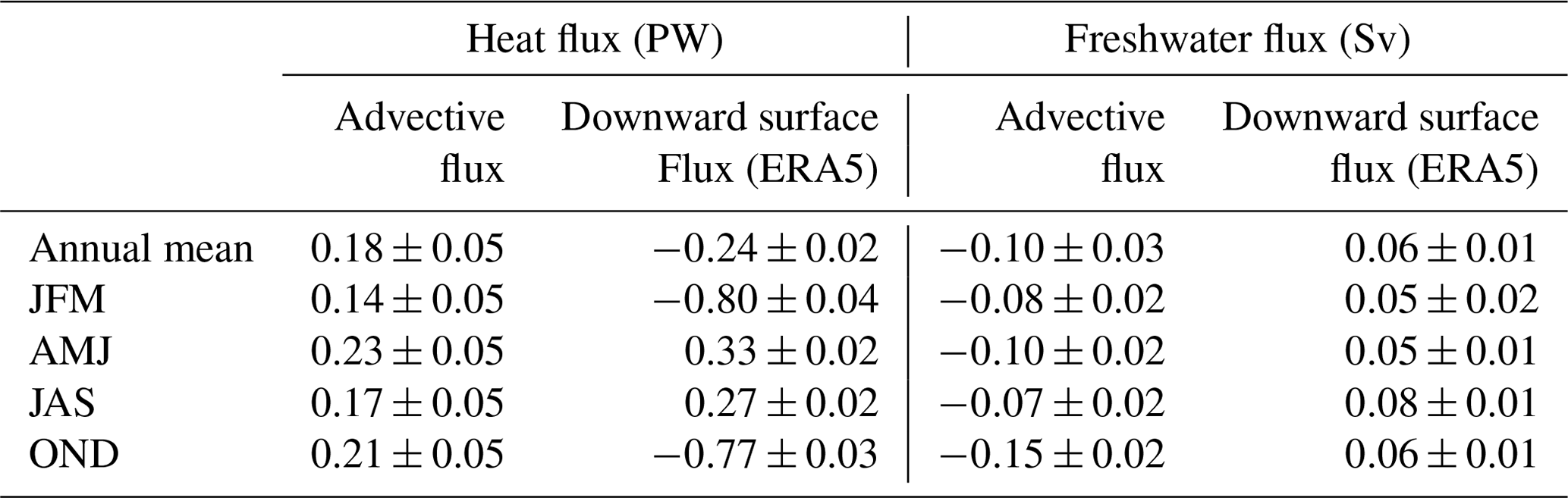
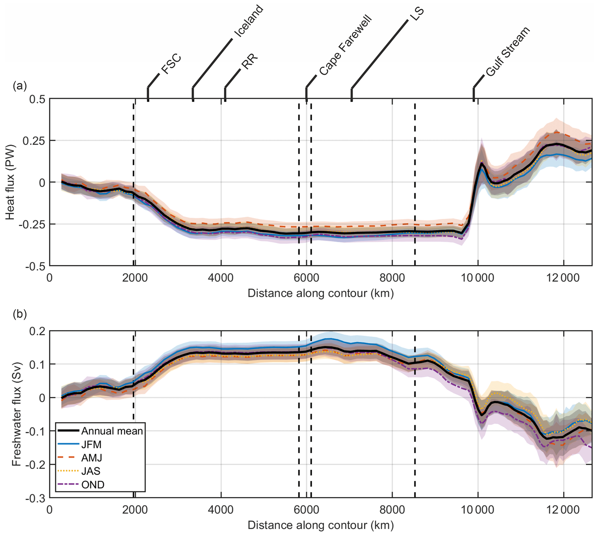
Figure 10Cumulative heat (PW) and fresh water (Sv) fluxes into the SPG between surface and seabed for (a) heat and (b) freshwater, using corrected velocities for sub-1000 m currents. Key locations around the boundary are labelled as in Fig. 3, and vertical dashed lines denote OSNAP crossings.
3.5 Heat and freshwater fluxes between the subpolar gyre and the boundary
3.5.1 Advective fluxes
The SPG on average gains heat of 0.18 ± 0.05 PW via advection (Fig. 10, Table 3). A total of 0.25 PW is exported across the Iceland–Scotland Ridge, in broad agreement with the estimate of Chafik and Rossby (2019) (0.27 PW, including Denmark Strait). A total of 0.4 PW is gained across 47∘ N, mainly in the Gulf Stream and NAC. Over much of the boundary little heat is exchanged with the exterior because the temperatures are close to the reference temperature (4.03 ∘C, Eq. 5). There is some heat loss to the exterior between 0 and 1000 km due to outflow combined with above-average temperatures. There is very little seasonality in heat flux across the 1000 m contour (0–9500 km).
Advection drives a net salinification of the SPG, with a net freshwater loss of −0.10 Sv. Freshwater flux is largely into the SPG up to 6500 km, driven by the net export of waters with salinity higher than the reference salinity. The NAC is responsible for the effective gain of 0.1 Sv of freshwater due to this effect. As for heat flux, there is little seasonality in freshwater flux around the boundary. An exception is off south-western Greenland, where fresher upper waters during the winter (Fig. S2 in the Supplement), in conjunction with increased surface Ekman transport (Fig. 6), do result in a localised seasonal gain of 0.02 Sv. Between the western Labrador Sea and the Flemish Cap about 0.08 Sv of freshwater is exported from the SPG before reaching 47∘ N. The effective negative freshwater flux of the Gulf Stream (−0.1 Sv) is the result of a positive volume flux associated with water of higher salinity than the basin-mean (, Eq. 6).
The local heat and freshwater fluxes and their signs depend on the reference values and used (Eqs. 5 and 6). For heat flux we use the mean temperature of the waters of the full-depth SPG interior enclosed by the boundary (4.03 ∘C). The heat fluxes thus have a physical meaning in that they show the level to which these waters warm or cool the SPG. Similarly, for freshwater flux we use the mean salinity of the full-depth SPG interior (35.14 g kg−3), thus showing the level to which the boundary fluxes freshen or salinise the SPG. As the flux calculations use mass-balanced velocities, the net heat fluxes into the SPG (Table 3) are insensitive to the choice of reference temperature (Eq. 5), but the net freshwater fluxes retain some sensitivity to the reference salinity due to the denominator of Eq. (6).
Spatially integrated (net) advective heat and freshwater fluxes into the SPG are shown in Table 3. Heat fluxes into the SPG range from 0.14 PW in winter to 0.23 PW in spring. Freshwater fluxes are negative in all seasons and are between −0.07 Sv (summer) and −0.15 Sv (autumn).
3.5.2 Surface heat and freshwater fluxes
In Table 3 we also show the seasonal and annual mean surface heat and freshwater fluxes derived from ERA5. The seasonal range of surface heat fluxes is much larger than that of the advective fluxes; between −0.80 PW (lost to atmosphere) in the winter and 0.33 PW (gained from atmosphere) in the spring. The annual mean surface heat loss (−0.24 PW) is of a similar magnitude to the advective heat flux into the SPG. Seasonality in freshwater surface fluxes are weak, ranging from 0.05 Sv in winter and spring to 0.08 Sv in the summer with an annual mean of 0.06 Sv into the SPG.
3.5.3 Boundary topography and its relationship with turbulent eddy fluxes
Steeply sloping margins are known to be rich in eddy activity (Spall and Pickart, 2000; Brüggemann and Katsman, 2019). It is therefore conceivable that eddy exchange of both heat and freshwater may be significant contributors to SPG–boundary exchange. The slope angle of the SPG boundary and its relationship to the EKE along the 1000 m contour is shown in Fig. 11.
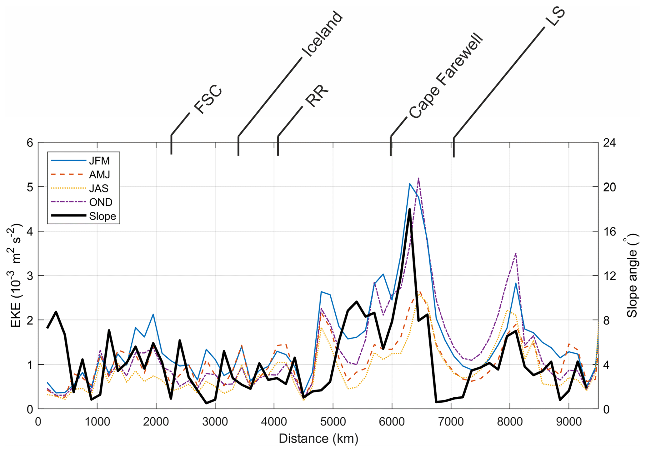
Figure 11Angle of continental slope (black) compared to EKE by region. Key locations around the boundary are labelled as in Fig. 3; note that the x axis excludes the 47∘ N transect.
The spatial distribution of EKE along the 1000 m contour appears relatively consistent between seasons, but during the autumn and winter EKE is about double that of spring and summer. EKE is greatest around Greenland and in the western Labrador Sea during all seasons, with the WGC values exceptionally high. The high EKE west of Greenland is consistent with previous studies (e.g. Fratantoni, 2001; Prater, 2002). A similar spatial structure emerges when examining the slope angle around the SPG boundary, with Fig. 11 showing the excellent agreement between the two parameters. Note that the extreme (>=20∘) slope west of Greenland corresponds to the EKE maximum in the WGC.
An estimate of the diffusive heat flux between the interior and exterior of the SPG associated with eddy activity was made using satellite-derived sea surface temperature (SST) and surface geostrophic velocities and is detailed in Sect. S4. Heat is diffused out of the SPG along the 1000 m contour, and into the SPG along 47∘ N (Fig. S3). A total of 0.0062 PW of heat energy enters the SPG via turbulent diffusion, roughly 2 orders of magnitude less than the contribution from advection, and therefore this process is not included in our heat budget. It was not possible to estimate diffusive freshwater flux due to the lack of reliable satellite sea surface salinity (SSS) observations.
In this article we present the first comprehensive observational assessment of properties, transports, and fluxes between the interior and exterior of the whole North Atlantic SPG. In conjunction with model data, we used this to identify the relative importance of processes driving fluxes across the boundary. Our observation-based approach uses data from 2000 to 2019, and thus can be considered the present mean state of circulation on decadal timescales. By considering fluxes into and out of the SPG as a whole, this work provides a measure of which processes in the SPG interior contribute to the AMOC.
4.1 Overturning in the subpolar gyre
Here we discuss the overturning stream function for the boundary of the SPG and what it implies for water mass transformation within the SPG.
We found the maximum of the annual mean overturning stream function in density space to be 7.36 ± 1.48 Sv across the 27.30 kg m−3 isopycnal (Table 2, Fig. 9a). To contextualise this value, the mean overturning measured across the 26∘ N zonal section by the RAPID-MOCHA array is 16.8 Sv (Smeed et al., 2018), while mean overturning across the ∼60∘ N OSNAP section, which bisects the SPG, is 16.6 Sv (Li et al., 2021a). Other estimates in the North Atlantic place the total overturning between 11.9 and 18.4 Sv (Caínzos et al., 2022; Fraser and Cunningham, 2021; Rossby et al., 2017; Sarafanov et al., 2012). Overturning estimates across the Greenland-Scotland Ridge vary from 5.5 to 5.7 Sv (Østerhus et al., 2019; Tsubouchi et al., 2021). However, estimates from transatlantic zonal sections only speak to water mass transformation north of the line in question. Our overturning stream function for a closed boundary (Fig. 9a) represents the excess inflow at lighter densities and excess outflow of denser water. We interpret these flows as water mass transformation in the interior of the SPG, an enclosed volume, and therefore as densification within the boundary (by surface fluxes). However, on seasonal timescales the inflow or outflow will be balanced by a combination of densification by surface fluxes and changing average density in the SPG. This density storage in the SPG interior will result in a lag before modified water is registered at the boundary curtain, thus attenuating the seasonal cycle in the overturning stream function.
Comparisons with other regionally bounded estimates of SPNA overturning are useful for interpreting our results dynamically. For example, our estimate for overturning is very similar to the overturning between OSNAP-East and the GSR estimated by Petit et al. (2020) (7.0 Sv). From this, one might infer that virtually all the overturning in the SPG happens in the Irminger and Iceland Basins. However, these estimates are not directly comparable for two reasons. Firstly, the domain covered by Petit et al. (2020) includes shallow and coastal regions comprising turbulent boundary currents and air–sea interactions over the East Greenland shelf, Reykjanes Ridge, and GSR, all of which are outside our domain. Secondly, Petit et al. (2020) estimate overturning in the interior by subtracting AMOC strength at the GSR from the AMOC strength at OSNAP-East, although these two overturning maxima do not necessarily coincide in density space, which may result in an underestimate of the actual overturning taking place in the region. On the other hand, our study finds a maximum overturning strength of 7.36 Sv across a common isopycnal, so the class of water mass transformation being quantified is consistent around the boundary. This is analogous to subtracting the overturning stream function at the GSR from the overturning stream function at OSNAP-East and taking the maximum value of the residual. While either approach might be considered a measure of overturning, the resulting values have different dynamical implications and are not directly comparable.
Our results reveal that the peak of the water mass transformation processes within the SPG occurs across the 27.30 kg m−3 isopycnal, substantially lighter than the density of maximum overturning north of OSNAP (27.66 kg m−3, Lozier et al., 2019). The net inflow at 47∘ N (Fig. 9c) is evenly distributed across a wide density range ( kg m−3), while the net outflow across the 1000 m isobath is concentrated around 27.35 kg m−3. The overturning maximum at σ0=27.30 kg m−3 therefore corresponds to the transformation of 7.36 Sv of upper water (σ0<27.3 kg m−3), which enters the SPG from the south before being cooled by the atmosphere to form SPMW (27.3–27.54 kg m−3). Around half (3.77 Sv) of this SPMW is then exported from the SPG (Fig. 9a) towards the Nordic Seas, where it is further transformed. This result supports the conclusions of Petit et al. (2020), who found roughly equal rates of deep-water formation in the north-eastern SPG and the Nordic Seas. As such, densification in the SPG preconditions further water mass transformation in the Nordic Seas and is thereby important for the North Atlantic overturning, but it is not appropriate to ascribe that part of the water mass transformation to overturning in the SPG. The transports by density layer (Fig. 8) reveal that the outflow in this (intermediate) density class is located between Iceland and Scotland, as it is carried northwards in the NAC.
The remaining SPMW is further transformed within the SPG, resulting in the broad plateau in the mean overturning between 27.4 to 27.6 kg m−3 with a secondary overturning maximum at σ0=27.54 kg m−3. This density range corresponds to isopycnals outcropping in the Irminger and Labrador seas (e.g. Lozier et al., 2019), indicating that this secondary transformation occurs as the remaining SPMW circulates into the western SPG. The resulting dense water (σ0>27.54 kg m−3) is then exported both via the Labrador Current and across 47∘ N (Fig. 8). Dense water also enters the SPG both at Cape Farewell, having presumably travelled south through the Denmark Strait in the EGC (e.g. Holliday et al., 2007) and in the Gulf Stream, which partially cancels the outflow at 47∘ N. However, the net export in this layer indicates dense water is formed, at a rate of 3.59 Sv, in the SPG interior.
The overturning maxima at σ0=27.30 and σ0=27.54 kg m−3 are both much lighter than the isopycnal of maximum overturning reported for OSNAP (27.66 kg m−3, Lozier et al., 2019) and are instead comparable with the outcropping isopycnals implicated in SPMW formation (27.3–27.5 kg m−3, Petit et al., 2021). This is because the GSR overflows that dominate the lower limb transport at OSNAP-East are formed outside of the SPG, and therefore contribute minimally to the overturning structure computed around our closed-loop boundary. The negative overturning values during autumn and winter (Fig. 9a) indicate that these overflow waters can become lighter inside the SPG. As the overflow waters in the Labrador Sea are too deep to be accessed by winter convection (Yashayaev, 2007), this modification probably occurs through mixing and entrainment with adjacent water masses.
The deepest overflows (σ0>27.8 kg m−3, Dickson and Brown, 1994) are not resolved by the boundary climatology (Fig. 3c). However, in reality these waters will flow southward through the SPG at depth with little exposure to the atmosphere. They therefore undergo minimal transformation within the SPG, meaning that their inclusion would not significantly alter the structure of overturning we observe (Fig. 9a). We address the issue of deep overflows in Sect. 4.5.
The maximum overturning at σ0≈27.30 kg m−3 has significant seasonal variability (Fig. 9a), with substantially larger values in winter and spring (9.33, 10.17 Sv) than in summer and autumn (6.59, 6.20 Sv). This is in accord with the seasonal overturning cycle now apparent north of OSNAP, such that overturning lags the winter surface cooling maximum by one season. For OSNAP, this lag results from surface Ekman forcing acting to reduce the northward transport in the upper layer during the winter due to the direction of prevailing winds relative to the transect (Li et al., 2021a; Petit et al., 2020, 2021). For our closed boundary, winter surface Ekman forcing has little impact on transport towards the Iceland–Scotland Ridge but maximally suppresses the import of upper-layer water (σ0<27.3 kg m−3) across the 47∘ N transect (Fig. 6). In addition, the winter mixed layer in the north-eastern Atlantic is too dense to contribute to the maximum overturning peak at σ0≈27.30 kg m−3. The net result of these influences is to delay the peak in overturning until spring. We find that removing surface Ekman forcing results in maximum overturning occurring during winter instead (not shown).
The secondary maximum in the overturning at σ0≈27.54 kg m−3 displays a different class of seasonal variability (Fig. 9a). The transformation is strongest in spring and summer (5.46, 5.31 Sv), while the autumn value (4.13 Sv) is close to the mean (3.59 Sv). In winter this secondary peak is absent, indicating that some of the SPMW formed in the eastern SPG is exported before undergoing further transformation to dense water (σ0>27.54 kg m−3). This may be due to the strong surface Ekman component in winter (Fig. 6) driving export of SPMW onto the shelf around the western Irminger and Labrador Basins.
In summary, we see 7.36 ± 1.48 Sv net import of upper waters (σ0<27.30 kg m−3), which are transformed in the interior and then exported, in approximately equal measure, as either intermediate water (27.30–27.54 kg m−3) in the NAC or as dense water (σ0>27.54 kg m−3) exiting to the south. These results support the findings of Petit et al. (2021) that the pre-conditioning of buoyant NAC waters into SPMW is a key stage in the transformation of water to successively higher densities and that it is therefore an important source of dense water masses for the lower limb of the AMOC.
4.2 Heat and freshwater divergence in the subpolar gyre
We find a net advective convergence of heat into the SPG of 0.18 ± 0.05 and a net divergence of freshwater of −0.10 ± 0.03 (Table 3). Are these compatible with atmospheric fluxes?
The annual mean net downward heat flux over the SPG is −0.24 ± 0.02 PW (Table 3). Thus, our estimate for the mean heat imported into the SPG through advection is approximately balanced by the mean loss to the atmosphere. The seasonal range of surface heat fluxes (−0.80 PW in the winter to 0.33 PW in the spring) is much greater than that for advective heat fluxes (0.14 PW in the winter to 0.23 PW in the spring). The annual mean net downward freshwater flux is 0.06 ± 0.01 Sv with only minor seasonality.
A discrepancy of −0.06 ± 0.07 PW remains between the rate of heat entering the SPG through advection and that of heat leaving the SPG through surface cooling averaged over 20 years. This value is compatible with the observed magnitude of cooling in the North Atlantic; for example, Bryden et al. (2020) find cooling at rate of 0.04 PW for the region 26–70∘ N between 2008 and 2016. For freshwater, the discrepancy between the rates of advective freshwater export and surface freshwater import (−0.04 ± 0.04 Sv) implies a net salinification during the period 2000–2019, which again supports the findings of Bryden et al. (2020), who reported freshwater loss at a rate of 0.062 Sv for the region 26–70∘ N between 2008 and 2016. We note that for both heat and freshwater fluxes, the discrepancy is within our error bounds so cannot be significantly distinguished from zero.
We find that a mean of 0.48 ± 0.05 PW crosses 47∘ N into the SPG (Fig. 10a). This is not directly comparable to other zonal transects (Fraser and Cunningham, 2021; Li et al., 2021b; Lozier et al., 2019) as our domain does not extend to the coast. However, we can estimate that if 0.48 PW is transported into the interior in the south and 0.18 PW is lost in the SPG, then 0.30 PW exits the SPG across the 1000 m contour. Similarly, a freshwater flux of −0.15 ± 0.03 Sv across 47∘ N (Fig. 10b) and a divergence of −0.10 Sv across the SPG implies a freshwater transport of 0.05 Sv across the 1000 m contour.
The heat entering via the Gulf Stream (0.3 ± 0.05 PW) reduces to 0.25 PW exiting via the Iceland–Scotland Ridge, suggesting that the NAC loses 0.05 PW of heat in the SPG. Similarly, the NAC gains freshwater at a rate of 0.01 ± 0.01 Sv in the SPG. It is interesting to note that substantial heat and freshwater is exchanged with the boundary south of the FSC (in the Rockall Trough), driving warming and salinification of the slope current, the NW European Shelf, and the North Sea.
The contribution of the energetic EGC and WGC systems to the overall SPG heat and freshwater budgets is relatively small. While the region around Greenland contributes up to 0.02 Sv of freshwater, the melting from the Greenland ice sheet appears to play a minor role in the freshwater budget of the SPG. This may be because much of the freshwater remains on the shelf rather than joining the EGC (De Steur et al., 2009). Near Cape Farewell, the ingress of 8 Sv of relatively dense water signals the import of various modified water masses across the Denmark Strait, entering the SPG chiefly through the EGC and WGC. The precise location of import is dependent on how our boundary intersects with the current cores and the EGC retroflection (e.g. Holliday et al., 2007), but the accumulated fluxes are robust to this effect. Net heat flux resulting from this interface is minimal because local temperatures are near the reference temperature (Fig. 10a, Eq. 5). Note that the impact of the poorly resolved overflows (see Sect. 4.5) on the SPG heat and freshwater budgets is likely to be minor. For example, an inflow of 3 Sv at 1 ∘C and 35 g kg−1 at the expected location of the DSO (e.g. Mastropole et al., 2017) results in a heat loss to the SPG of 0.04 PW, which is smaller than our error bounds, and a negligible gain in freshwater.
While turbulent diffusion does not play a significant role in the SPG heat budget, the highly energetic Gulf Stream eddy field does import 0.025 PW, or about 8 % of the total Gulf Stream heat input, though this is largely compensated for by heat leaving the SPG on either side (Fig. S3). This value is still an order of magnitude smaller than the eddy heat flux estimated at 36∘ N (immediately after its separation at Cape Hatteras) by Tréguier et al. (2017) (0.3 PW), though this is perhaps unsurprising given the profound change in the character of the Gulf Stream between 36 and 47∘ N.
4.3 Buoyancy exchanges in the western subpolar gyre
It is clear from Fig. 3 that density generally increases with progress around the SPG boundary and that this is primarily caused by gradual cooling. This reflects the buoyancy loss in the interior and is also seen in the boundary current as it flows around the basin (Straneo, 2006). A notable exception to the increasing density trend is south-western Greenland, where an injection of freshwater (and warming below 250 m) leads to a marked reduction in density, along with a reversal of volume transports between the interior of the SPG and the boundary in this region (Fig. 5). While Liu et al. (2022) diagnose upwelling in this region, instabilities in the WGC and the associated formation of Irminger rings (e.g. Fratantoni, 2001; Prater, 2002) would appear to be likely sources for this signal in our 1000 m contour climatology. We note that the reversal of the prevailing horizontal density gradient is a subtlety that is lacking from more idealised studies of boundary current dynamics that assume a continual decrease in density with progress anticlockwise around the SPG (e.g. Brüggemann and Katsman, 2019).
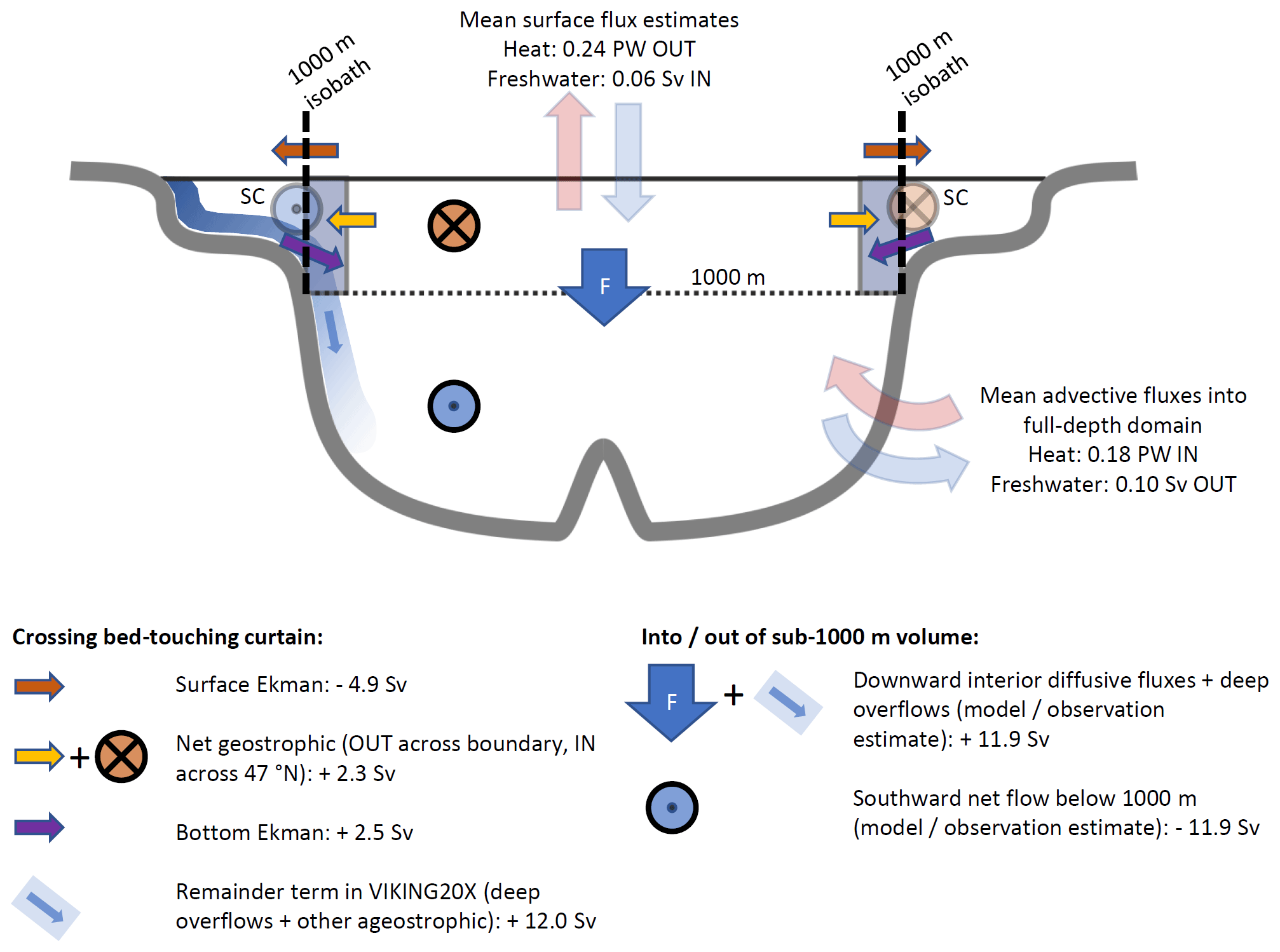
Figure 12Schematic of SPG boundary and interior processes contributing to transport through the SPG, viewed from 47∘ N section. The shaded rectangles on either side of the basin represent the regions in which CTD data were gathered. SC stands for slope current. Net flow across 47∘ N above 1000 m is northward (into the SPG), while below 1000 m it is southward (out of the SPG). A net downwelling (F) is required to balance the transports in and out of the SPG.
The role of the EGC and WGC in water mass modification is undoubtedly enhanced by eddy activity, which is in part driven by the boundary current interacting with local topography. In Fig. 11 we show that the exceptionally high EKE values in the WGC region are associated with a slope of 20∘ W of Greenland. This coherence suggests that EKE, and hence the diffusive flux of buoyancy between the boundary and SPG, is controlled by the steepness of the sloping margins. As we have already stated, diffusive fluxes have minimal significance for the overall boundary heat and freshwater budget, but in the WGC region we find that diffusive and advective fluxes are comparable. Studies citing eddy diffusion for communication between interior and boundary tend to be located around southern Greenland (Brüggemann and Katsman, 2019; Le Bras et al., 2020; Liu et al., 2022), and our results highlight that this region is an exception to the rule around the gyre.
We do not see clear signs of true winter deep convection at the boundary of the Labrador Sea (Fig. S2, mixed layer depths of >800 m are indicated by Lavender et al., 2000). While the boundary current system was ventilated during the severe winters of the early and mid-1990s (Pickart et al., 1997), these episodes occurred outside our data's temporal coverage (2000 onwards). Deep convection appears to have been largely confined to the basin interior in recent winters, communicated to the boundary and appearing as anomalies at the boundary in spring (Yashayaev and Loder, 2017, Fig. S2).
4.4 Subpolar gyre volume budget estimation
Given the transports estimated in this study, we can make a first-order estimate of the SPG volume budget given the continuity constraint of zero net transport.
The SPG interior can be divided into an upper and lower volume partitioned at 1000 m depth. The upper volume is enclosed by the 1000 m boundary curtain and the 47∘ N section, the lower volume is completely enclosed except across 47∘ N (Fig. 12). A net inflow above 1000 m must be balanced by downwelling across the 1000 m “surface”. In addition, model-based estimates of the North Atlantic AMOC in depth space find maximum overturning located near 1000 m (Biastoch et al., 2021; Hirschi et al., 2020), and thus the vertical transport across 1000 m is approximately equivalent to the strength of the AMOC in the SPG. This balance is depicted in Eq. (10):
The Qinflow<1000 m term can be expressed as the sum of the geostrophic, surface Ekman, and bottom Ekman transports, with a remainder term necessary to capture flows not resolved by the observational budget:
Net geostrophic flow above 1000 m is only permitted due to the beta effect and is therefore constrained (mean +2.3 Sv). Note that this would be the case even if the hydrography were perfectly known. For surface Ekman we take the annual mean calculated from observations (−4.9 Sv, Sect. 3.2.2). For bottom Ekman we use the estimate from Argo trajectories (+2.5 Sv, Sect. 3.2.3). Given the approximate cancellation of the mean geostrophic, surface Ekman, and bottom Ekman terms (totalling −0.1 Sv), Qremainder is left as the dominant term on the right-hand side. Thus, on average, almost all the southward flow below 1000 m at 47∘ N is driven by the Qremainder term. Note that the sum of geostrophic, surface Ekman, and bottom Ekman terms is seasonal (+2.35 Sv in summer, −2.9 Sv in winter), with the seasonality driven by the surface Ekman term (Table 1). We might therefore state that, on average,
Hence from Eqs. (10) and (12),
We estimate the mean Qremainder to be 12.0 Sv using VIKING20X (dashed grey line, Fig. 7b). From Eq. (11), this results in a net gain of +11.9 Sv above 1000 m, necessitating a downwelling flow of 11.9 Sv through the 1000 m surface, and an equivalent southward net flow across 47∘ N below 1000 m (Fig. 12). The depth space AMOC estimated by Hirschi et al. (2020) and Biastoch et al. (2021) is 10–15 Sv and therefore is of the same order as that inferred from the VIKING20X remainder term.
4.5 The role of unresolved flows
Between the UK and Greenland (Fig. 5) 12 Sv of geostrophic transport leaves the SPG. This is the same transport as was reported for the upper limb across OSNAP-East (Lozier et al., 2019) and implies that the return current in the lower limb is not captured in the geostrophic transports from the observational analysis. Another indication that the lower limb of the AMOC is not fully resolved in the observations is the lack of very cold (<3 ∘C) and dense (>27.8 kg m−3) waters where we would expect the Faroe Bank Channel overflow and DSO to bisect the boundary (Johnson et al., 2017; Mastropole et al., 2017). The dominant role of Qremainder in Sect. 4.4 further highlights that some processes are not fully captured by the observational analysis. In this section we consider which regions and dynamical processes contribute to the Qremainder term.
The region off south-eastern Greenland is responsible for over half the Qremainder signal in VIKING20X (Fig. 7). We surmise that the modelled DSO is primarily responsible for this transport. The model fields suggest a contribution by Qremainder of 6.0–6.8 Sv entering the SPG in the Denmark Strait region, with the majority of the flow close to the seabed (dashed grey line, Fig. 7). For comparison, observational estimates of the volume transport in the overflow indicate that the DSO is responsible for 3.2–3.5 Sv (Girton et al., 2001; Harden et al., 2016; Jochumsen et al., 2012, 2017; Käse et al., 2003). The transport across the sill may then roughly double by entrainment as the dense water descends toward the abyssal plain (Dickson and Brown, 1994). By contrast, observational estimates of the Faroe Bank Channel overflow suggest an underestimation of its flow in VIKING20X (2.6 Sv, Johns et al., 2021). The volume transport of the overflows into the SPG interior in VIKING20X may therefore be approximately correct, although their physics and relative contributions are probably not simulated very realistically.
We have encountered modelling results suggesting that the overflows may have a significant ageostrophic and non-Ekman component and must therefore receive significant contributions from non-linear and viscous processes. For example, the DSO is manifested as a turbulent cascade released over the sill in pulses with a timescale of around 3–5 d (e.g. Käse et al., 2003; Lin et al., 2020; Spall et al., 2019). One would anticipate that small-scale, non-linear, and ageostrophic processes would dominate in such an environment. It is beyond the scope of this paper to quantitatively assess these processes. However, our analysis demonstrates the importance of overflow dynamics in closing the overturning streamlines in the SPNA.
There are several reasons why our sampling strategy and analysis may result in poorly resolved overflows. Firstly, the relatively low horizontal resolution along the boundary contour may be too coarse to clearly resolve overflow waters in the gridded profile data. Secondly, the profiles contributing to our dataset may on average be too far from the continental slope to regularly capture the overflow (see schematic in Fig. 12). Thirdly, due to the transitory nature of the overflow waters, temporally scattered CTD sampling may fail to sample them. Finally, Argo floats may be actively deflected around the downslope-flowing boluses of dense water, and thus do not sample the core properties.
A novel observational climatology of the entire SPG boundary has yielded new perspectives on overturning in the interior of the SPG. We find an average transformation of 7.36 ± 1.48 Sv of upper waters (σ0<27.30 kg m−3) occurs within the SPG, with a seasonal maximum in spring and minimum in the autumn, lagging surface buoyancy forcing by one season. The products of upper-water transformation are intermediate water (27.30–27.54 kg m−3) exiting in the NAC into the Nordic Seas or dense water (σ0>27.54 kg m−3) exiting to the south. These findings underline the findings of Petit et al. (2021) that the overturning of dense waters is reliant on the prior “pre-conditioning” of lighter waters.
We find a mean advective convergence of heat into the SPG of 0.18 ± 0.05 W and a net divergence of freshwater of −0.10 ± 0.02 Sv, which are approximately balanced by surface fluxes. Net diffusive heat and freshwater fluxes into the SPG are negligible, but hotspots of eddy activity such as the Gulf Stream and western Greenland result in localised diffusive heat fluxes approaching those of the advective contributions.
When considering the total transports into and out of the SPG volume, we find that the mean geostrophic (2.3 Sv), surface Ekman (−4.9 Sv), and bottom Ekman (2.5 Sv) terms approximately cancel, meaning that flow downwards across the 1000 m surface is dominated by ageostrophic (and non-Ekman) processes. This result highlights the requirement to better understand the overflows into the SPG and the net sinking that occurs along the boundary (e.g. Johnson et al., 2019; Spall and Pickart, 2000) and demonstrates that a geostrophic approach alone may not be sufficient for this.
Our investigation focused on the recent (20-year) climatic mean state, as was necessitated by observational data availability. However, given recent evidence of changes in large-scale circulation patterns (Biastoch et al., 2021; Fox et al., 2022; Zhang and Thomas, 2021), it is crucial to assess the decadal shifts in the basin-scale processes outlined here and establish to what extent this can alter the behaviour of the AMOC.
Aggregated Argo and CTD profile data are available from the WOD at https://www.ncei.noaa.gov/access/world-ocean-database-select/dbsearch.html (last access: 3 September 2019, Boyer et al., 2018). EN.4.2.2 data (bias corrections .g10, downloaded 4 March 2021) were obtained from https://www.metoffice.gov.uk/hadobs/en4/, and are Crown Copyright, Met Office, 2022, provided under a Non-Commercial Government Licence, http://www.nationalarchives.gov.uk/doc/non-commercial-government-licence/version/2/ (last access: 4 March 2021, Good et al., 2013; Gouretski and Reseghetti, 2010; Gouretski and Cheng, 2020). ECMWF reanalysis data are available through the Copernicus Marine Environment Monitoring Service (CMEMS, 2022, https://marine.copernicus.eu/, last access: 6 April 2022, Hersbach et al., 2019). Satellite altimetry data are available through the Copernicus Marine Environment Monitoring Service (CMEMS, 2020, https://marine.copernicus.eu/, product identifier: SEALEVEL_GLO_PHY_L4_MY_008_047, last access: 1 December 2020, Copernicus Climate Change Service (C3S), 2018). GEBCO bathymetry data can be downloaded from https://doi.org/10.5285/836f016a-33be-6ddc-e053-6c86abc0788e (last access: 15 June 2020, GEBCO Compilation Group 2019). The code for computing fluxes and overturning from the boundary climatology is available at https://doi.org/10.5281/zenodo.7566026 (last access: 24 January 2023, Jones, 2023). The NEMO code used (version 3.6, revision 6721) is available at https://zenodo.org/record/3248739 (last access: 16 May 2022, Gurvan et al., 2017). The original underlying VIKING20X model output is available on request from GEOMAR research data management (datamanagement@geomar.de).
The supplement related to this article is available online at: https://doi.org/10.5194/os-19-169-2023-supplement.
SCJ conducted the core analyses and prepared the manuscript with contributions from all co-authors. NJF computed the surface Ekman transports and EKE values around the boundary and contributed to manuscript preparation and interpretation of results. SAC secured the funding for the work, conceptualised the gyre boundary investigation, and contributed to the text and experiment design throughout. ADF supplied the VIKING20X investigation and contributed to the text and interpretation of results. MEI supplied the slope angle investigation and contributed to the text and interpretation of results.
The contact author has declared that neither of the authors has any competing interests.
Publisher's note: Copernicus Publications remains neutral with regard to jurisdictional claims in published maps and institutional affiliations.
We are grateful for the helpful suggestions by two anonymous reviewers which undoubtedly strengthened this paper.
This project was supported by the NERC research programme funding CLASS NE/R015953/1, OSNAP NE/K010700/1, and SNAP-DRAGON NE/T013494/1 (Neil J. Fraser and Stuart A. Cunningham). Additional support (Alan D. Fox) was received from the European Union Horizon 2020 Research and Innovation Programme under grant no. 727852 (Blue-Action). This output reflects only the authors' views and the European Union cannot be held responsible for any use that may be made of the information contained therein.
This paper was edited by Karen J. Heywood and reviewed by two anonymous referees.
Barnier, B., Madec, G., Penduff, T., Molines, J.M., Treguier, A.M., Le Sommer, J., Beckmann, A., Biastoch, A., Böning, C., Dengg, J., and Derval, C.: Impact of partial steps and momentum advection schemes in a global ocean circulation model at eddy-permitting resolution, Ocean Dynam., 56, 543–567, https://doi.org/10.1007/s10236-006-0082-1, 2006.
Berx, B., Hansen, B., Østerhus, S., Larsen, K. M., Sherwin, T., and Jochumsen, K.: Combining in situ measurements and altimetry to estimate volume, heat and salt transport variability through the Faroe–Shetland Channel, Ocean Sci., 9, 639–654, https://doi.org/10.5194/os-9-639-2013, 2013.
Biastoch, A., Schwarzkopf, F. U., Getzlaff, K., Rühs, S., Martin, T., Scheinert, M., Schulzki, T., Handmann, P., Hummels, R., and Böning, C. W.: Regional imprints of changes in the Atlantic Meridional Overturning Circulation in the eddy-rich ocean model VIKING20X, Ocean Sci., 17, 1177–1211, https://doi.org/10.5194/os-17-1177-2021, 2021.
Boyer, T. P., Baranova, O. K., Coleman, C., Garcia, H. E., Grodsky, A., Locarnini, R. A., Mishonov, A. V., Paver, C.R., Reagan, J. R., Seidov, D., Smolyar, I. V., Weathers, K., and Zweng, M. M.: World Ocean Database 2018, NOAA Atlas NESDIS 87 [data set], https://www.ncei.noaa.gov/access/world-ocean-database-select/dbsearch.html (last access: 3 September 2019), 2018.
Brambilla, E. and Talley, L. D.: Subpolar Mode Water in the northeastern Atlantic: 1. Averaged properties and mean circulation, J. Geophys. Res.-Oceans, 113, C04025, doi:10.1029/2006JC004062, 2008.
Brambilla, E., Talley, L. D., and Robbins, P. E.: Subpolar mode water in the northeastern Atlantic: 2. Origin and transformation, J. Geophys. Res.-Oceans, 113, C04026, doi:10.1029/2006JC004063, 2008.
Brüggemann, N. and Katsman, C. A.: Dynamics of downwelling in an eddying marginal sea: Contrasting the Eulerian and the isopycnal perspective, J. Phys. Oceanogr., 49, 3017–3035, https://doi.org/10.1175/JPO-D-19-0090.1, 2019.
Bryden, H. L., Johns, W. E., King, B. A., McCarthy, G., McDonagh, E. L., Moat, B. I., and Smeed, D. A.: Reduction in ocean heat transport at 26∘ N since 2008 cools the eastern subpolar gyre of the North Atlantic Ocean, J. Climate, 33, 1677–1689, https://doi.org/10.5194/os-16-863-2020, 2020.
Caínzos, V., Hernández-Guerra, A., McCarthy, G.D., McDonagh, E.L., Cubas Armas, M., and Pérez-Hernández, M. D.: Thirty years of GOSHIP and WOCE data: Atlantic overturning of mass, heat, and freshwater transport, Geophys. Res. Lett., 49, e2021GL096527, https://doi.org/10.1029/2021GL096527, 2022.
GEBCO Compilation Group: GEBCO 2019 Grid, GEBCO [data set], https://doi.org/10.5285/836f016a-33be-6ddc-e053-6c86abc0788e, 2019.
Chafik, L. and Rossby, T.: Volume, heat, and freshwater divergences in the subpolar North Atlantic suggest the Nordic Seas as key to the state of the meridional overturning circulation, Geophys. Res. Lett., 46, 4799–4808, https://doi.org/10.1029/2019GL082110, 2019.
Chen, X. and Tung, K. K.: Varying planetary heat sink led to global-warming slowdown and acceleration, Science, 345, 897–903, https://doi.org/10.1126/science.1254937, 2014.
Copernicus Climate Change Service (C3S): Climate Data Store: Sea level daily gridded data from satellite observations for the global ocean from 1993 to present. Copernicus Climate Change Service (C3S) Climate Data Store (CDS) [data set], doi:10.24381/cds.4c328c78, 2018.
Davis, R. E.: Preliminary results from directly measuring middepth circulation in the tropical and South Pacific, J. Geophys. Res.-Oceans, 103, 24619–24639, https://doi.org/10.1029/98JC01913, 1998.
De Jong, M. F., Oltmanns, M., Karstensen, J., and De Steur, L.: Deep Convection in the Irminger Sea observed with a dense mooring array, Oceanography, 31, 50–59, 2018.
De Steur, L., Hansen, E., Gerdes, R., Karcher, M., Fahrbach, E., and Holfort, J.: Freshwater fluxes in the East Greenland Current: A decade of observations, Geophys. Res. Lett., 36, L23611, https://doi.org/10.1029/2009GL041278, 2009.
De Steur, L., Pickart, R.S., Macrander, A., Våge, K., Harden, B., Jónsson, S., Østerhus, S., and Valdimarsson, H.: Liquid freshwater transport estimates from the East Greenland Current based on continuous measurements north of Denmark Strait, J. Geophys. Res.-Oceans, 122, 93–109, https://doi.org/10.1002/2016JC012106, 2017.
Desbruyères, D. G., Sinha, B., McDonagh, E. L., Josey, S. A., Holliday, N. P., Smeed, D. A., New, A. L., Megann, A., and Moat, B. I.: Importance of boundary processes for heat uptake in the subpolar North Atlantic, J. Geophys. Res.-Oceans, 125, e2020JC016366, https://doi.org/10.1029/2020JC016366, 2020.
Dickson, R. R. and Brown, J.: The production of North Atlantic Deep Water: sources, rates, and pathways, J. Geophys. Res.-Oceans, 99, 12319–12341, https://doi.org/10.1029/94JC00530, 1994.
Dickson, B., Dye, S., Jónsson, S., Köhl, A., Macrander, A., Marnela, M., Meincke, J., Olsen, S., Rudels, B., Valdimarsson, H., and Voet, G.: The overflow flux west of Iceland: Variability, origins and forcing, in Arctic-Subarctic Ocean Fluxes: Defining the Role of the Northern Seas in Climate, Springer Netherlands, 443–474, 2008.
Fox, A. D., Handmann, P., Schmidt, C., Fraser, N., Rühs, S., Sanchez-Franks, A., Martin, T., Oltmanns, M., Johnson, C., Rath, W., Holliday, N. P., Biastoch, A., Cunningham, S. A., and Yashayaev, I.: Exceptional freshening and cooling in the eastern subpolar North Atlantic caused by reduced Labrador Sea surface heat loss, Ocean Sci., 18, 1507–1533, https://doi.org/10.5194/os-18-1507-2022, 2022.
Fraser, N. J. and Cunningham, S. A.: 120 years of AMOC variability reconstructed from observations using the Bernoulli inverse, Geophys. Res. Lett., 48, e2021GL093893, https://doi.org/10.1029/2021GL093893, 2021.
Fratantoni, D. M.: North Atlantic surface circulation during the 1990's observed with satellite-tracked drifters, J. Geophys. Res.-Oceans, 106, 22067–22093, https://doi.org/10.1029/2000JC000730, 2001.
GEBCO Compilation Group: GEBCO 2019 Grid, GEBCO [data set], https://doi.org/10.5285/836f016a-33be-6ddc-e053-6c86abc0788e, 2019.
Girton, J. B., Sanford, T. B., and Käse, R. H.: Synoptic sections of the Denmark Strait overflow, Geophys. Res. Lett., 28, 1619–1622, 2001.
Good, S. A., Martin, M. J., and Rayner, N. A.: EN4: Quality controlled ocean temperature and salinity profiles and monthly objective analyses with uncertainty estimates, J. Geophys. Res.-Oceans, 118, 6704–6716, 2013.
Good, S. A., Martin, M. J., and Rayner, N. A.: EN4: Quality controlled ocean temperature and salinity profiles and monthly objective analyses with uncertainty estimates, J. Geophys. Res.-Oceans, 118, 6704–6716, https://doi.org/10.1002/2013JC009067, 2013.
Gouretski, V. and Reseghetti, F.: On depth and temperature biases in bathythermograph data: Development of a new correction scheme based on analysis of a global ocean database, Deep Sea Res. Pt. I, 57, 812–833, https://doi.org/10.1016/J.DSR.2010.03.011, 2010.
Gouretski, V. and Cheng, L.: Correction for Systematic Errors in the Global Dataset of Temperature Profiles from Mechanical Bathythermographs, J. Atmos. Ocean. Tech., 37, 841–855, https://doi.org/10.1175/JTECH-D-19-0205.1, 2020.
Gurvan, M., Bourdallé-Badie, R., Bouttier, P.-A., Bricaud, C., Bruciaferri, D., Calvert, D., Chanut, J., Clementi, E., Coward, A., Delrosso, D., Ethé, C., Flavoni, S., Graham, T., Harle, J., Iovino, D., Lea, D., Lévy, C., Lovato, T., Martin, N., Masson, S., Mocavero, S., Paul, J., Rousset, C., Storkey, D., Storto, A., and Vancoppenolle, M.: NEMO ocean engine, Zenodo [code], https://doi.org/10.5281/zenodo.3248739, 2017.
Hansen, B., Larsen, K. M. H., Hátún, H., Kristiansen, R., Mortensen, E., and Østerhus, S.: Transport of volume, heat, and salt towards the Arctic in the Faroe Current 1993–2013, Ocean Sci., 11, 743–757, https://doi.org/10.5194/os-11-743-2015, 2015.
Harden, B. E., Pickart, R. S., Valdimarsson, H., Våge, K., de Steur, L., Richards, C., Bahr, F., Torres, D., Børve, E., Jónsson, S., and Macrander, A.: Upstream sources of the Denmark Strait Overflow: Observations from a high-resolution mooring array, Deep-Sea Res. Pt. I, 112, 94–112, https://doi.org/10.1016/j.dsr.2016.02.007, 2016.
Hersbach, H., Bell, B., Berrisford, P., Biavati, G., Horányi, A., Muñoz Sabater, J., Nicolas, J., Peubey, C., Radu, R., Rozum, I., Schepers, D., Simmons, A., Soci, C., Dee, D., and Thépaut, J.-N.: ERA5 monthly averaged data on single levels from 1959 to present. Copernicus Climate Change Service (C3S) Climate Data Store (CDS) [data set], doi:10.24381/cds.f17050d7, 2019.
Hersbach, H., Bell, B., Berrisford, P., Hirahara, S., Horányi, A., Muñoz-Sabater, J., Nicolas, J., Peubey, C., Radu, R., Schepers, D., and Simmons, A.: The ERA5 global reanalysis, Q. J. Roy. Meteor. Soc., 146, 1999–2049, 2020.
Hirschi, J. J. M., Barnier, B., Böning, C., Biastoch, A., Blaker, A. T., Coward, A., Danilov, S., Drijfhout, S., Getzlaff, K., Griffies, S. M., and Hasumi, H.: The Atlantic meridional overturning circulation in high-resolution models, J. Geophys. Res.-Oceans, 125, e2019JC015522, https://doi.org/10.1029/2019JC015522, 2020.
Holliday, N. P., Meyer, A., Bacon, S., Alderson, S. G., and de Cuevas, B.: Retroflection of part of the east Greenland current at Cape Farewell, Geophys. Res. Lett., 34, 7609, https://doi.org/10.1029/2006GL029085, 2007.
Huthnance, J. M., Inall, M. E., and Fraser, N. J.: Oceanic density/pressure gradients and slope currents, J. Phys. Oceanogr., 50, 1643–1654, https://doi.org/10.1175/JPO-D-19-0134.1, 2020.
Huthnance, J., Hopkins, J., Berx, B., Dale, A., Holt, J., Hosegood, P., Inall, M., Jones, S., Loveday, B. R., Miller, P. I., and Polton, J.: Ocean shelf exchange, NW European shelf seas: Measurements, estimates and comparisons, Prog. Oceanogr., 202, 102760, https://doi.org/10.1016/j.pocean.2022.102760, 2022.
Jochumsen, K., Quadfasel, D., Valdimarsson, H. and Jónsson, S.: Variability of the Denmark Strait overflow: Moored time series from 1996–2011, J. Geophys. Res.-Oceans, 117, C12003, https://doi.org/10.1029/2012JC008244, 2012.
Jochumsen, K., Moritz, M., Nunes, N., Quadfasel, D., Larsen, K.M., Hansen, B., Valdimarsson, H., and Jonsson, S.: Revised transport estimates of the D enmark S trait overflow, J. Geophys. Res.-Oceans, 122, 3434–3450, https://doi.org/10.1002/2017JC012803, 2017.
Johns, W. E., Devana, M., Houk, A., and Zou, S.: Moored Observations of the Iceland-Scotland Overflow Plume Along the Eastern Flank of the Reykjanes Ridge, J. Geophys. Res.-Oceans, 126, e2021JC017524, https://doi.org/10.1029/2021JC017524, 2021.
Johnson, C., Sherwin, T., Cunningham, S., Dumont, E., Houpert, L., and Holliday, N. P.: Transports and pathways of overflow water in the Rockall Trough, Deep-Sea Res. Pt. I, 122, 48–59, https://doi.org/10.1016/j.dsr.2017.02.004, 2017.
Johnson, H. L., Cessi, P., Marshall, D. P., Schloesser, F., and Spall, M. A.: Recent contributions of theory to our understanding of the Atlantic meridional overturning circulation, J. Geophys. Res.-Oceans, 124, 5376–5399, https://doi.org/10.1029/2019JC015330, 2019.
Jones, S., Cottier, F., Inall, M., and Griffiths, C.: Decadal variability on the Northwest European continental shelf, Prog. Oceanogr., 161, 131–151, https://doi.org/10.1016/j.pocean.2018.01.012, 2018.
Jones, S., Inall, M., Porter, M., Graham, J. A., and Cottier, F.: Storm-driven across-shelf oceanic flows into coastal waters, Ocean Sci., 16, 389–403, https://doi.org/10.5194/os-16-389-2020, 2020.
Jones, S. C.: Code used in transport and flux analysis for Jones et al. 2023. “Observation-based estimates of volume, heat and freshwater exchanges between the subpolar North Atlantic interior, its boundary currents and the atmosphere”, Zenodo [code], doi:10.5281/zenodo.7566026, 2023.
Josey, S. A., Jong, M. F., Oltmanns, M., Moore, G. K., and Weller, R. A.: Extreme variability in Irminger Sea winter heat loss revealed by ocean observatories initiative mooring and the ERA5 reanalysis, Geophys. Res. Lett., 46, 293–302, https://doi.org/10.1029/2018GL080956, 2019.
Käse, R. H., Girton, J. B., and Sanford, T. B.: Structure and variability of the Denmark Strait Overflow: Model and observations, J. Geophys. Res.-Oceans, 108, 3181, doi:10.1029/2002JC001548, 2003.
Kostov, Y., Johnson, H. L., Marshall, D. P., Heimbach, P., Forget, G., Holliday, N. P., Lozier, M. S., Li, F., Pillar, H. R., and Smith, T.: Distinct sources of interannual subtropical and subpolar Atlantic overturning variability, Nat. Geosci., 14, 491–495, https://doi.org/10.1038/s41561-021-00759-4, 2021.
Laurila, T. K., Sinclair, V. A., and Gregow, H.: Climatology, variability, and trends in near-surface wind speeds over the North Atlantic and Europe during 1979–2018 based on ERA5, Int. J. Climatol., 41, 2253–2278, https://doi.org/10.1002/joc.6957, 2021.
Lavender, K. L., Davis, R. E., and Owens, W. B.: Mid-depth recirculation observed in the interior Labrador and Irminger seas by direct velocity measurements, Nature, 407, 66–69, 2000.
Le Bras, I. A., Straneo, F., Holte, J., De Jong, M. F., and Holliday, N. P.: Rapid export of waters formed by convection near the Irminger Sea's western boundary, Geophys. Res. Lett., 47, e2019GL085989, https://doi.org/10.1029/2019GL085989, 2020.
Li, F. and Lozier, M. S.: On the linkage between Labrador Sea Water volume and overturning circulation in the Labrador Sea: A case study on proxies, J. Climate, 31, 5225–5241, https://doi.org/10.1175/JCLI-D-17-0692.1, 2018.
Li, F., Lozier, M. S., Bacon, S., Bower, A. S., Cunningham, S. A., de Jong, M. F., deYoung, B., Fraser, N., Fried, N., Han, G., Holliday, N. P., Holte, J., Houpert, L., Inall, M. E., Johns, W. E., Jones, S., Johnson, C., Karstensen, J., Le Bras, I. A., Lherminier, P., Lin, X., Mercier, H., Oltmanns, M., Pacini, A., Petit, T., Pickart, R. S., Rayner, D., Straneo, F., Thierry, V., Visbeck, M., Yashayaev, I., and Zhou, C.: Subpolar North Atlantic western boundary density anomalies and the Meridional Overturning Circulation, Nat. Commun., 12, 3002, https://doi.org/10.1038/s41467-021-23350-2, 2021a.
Li, F., Lozier, M. S., Holliday, N. P., Johns, W. E., Le Bras, I. A., Moat, B. I., Cunningham, S. A., and De Jong, M. F.: Observation-based estimates of heat and freshwater exchanges from the subtropical North Atlantic to the Arctic, Prog. Oceanogr., 197, 102640, https://doi.org/10.1016/j.pocean.2021.102640, 2021b.
Lin, P., Pickart, R. S., Torres, D. J., and Pacini, A.: Evolution of the freshwater coastal current at the southern tip of Greenland, J. Phys. Oceangr., 48, 2127–2140, https://doi.org/10.1175/JPO-D-18-0035.1, 2018.
Lin, P., Pickart, R. S., Jochumsen, K., Moore, G. W. K., Valdimarsson, H., Fristedt, T., and Pratt, L. J.: Kinematic structure and dynamics of the Denmark Strait overflow from ship-based observations, J. Phys. Oceangr., 50, 3235–3251, https://doi.org/10.1175/JPO-D-20-0095.1, 2020.
Liu, Y. J., Desbruyères, D. G., Mercier, H., and Spall, M. A.: Observation-based estimates of Eulerian-mean boundary downwelling in the western subpolar North Atlantic, Geophys. Res. Lett., 49, e2021GL097243, https://doi.org/10.1029/2021GL097243, 2022.
Lozier, M. S., Li, F., Bacon, S., Bahr, F., Bower, A. S., Cunningham, S. A., De Jong, M. F., De Steur, L., DeYoung, B., Fischer, J., Gary, S. F., Greenan, B. J. W., Holliday, N. P., Houk, A., Houpert, L., Inall, M. E., Johns, W. E., Johnson, H. L., Johnson, C., Karstensen, J., Koman, G., Le Bras, I. A., Lin, X., Mackay, N., Marshall, D. P., Mercier, H., Oltmanns, M., Pickart, R. S., Ramsey, A. L., Rayner, D., Straneo, F., Thierry, V., Torres, D. J., Williams, R. G., Wilson, C., Yang, J., Yashayaev, I., and Zhao, J.: A sea change in our view of overturning in the subpolar North Atlantic, Science, 363, 516–521, https://doi.org/10.1126/science.aau6592, 2019.
Marsh, R., Haigh, I. D., Cunningham, S. A., Inall, M. E., Porter, M., and Moat, B. I.: Large-scale forcing of the European Slope Current and associated inflows to the North Sea, Ocean Sci., 13, 315–335, https://doi.org/10.5194/os-13-315-2017, 2017.
Masson-Delmotte, V., Zhai, P., Pirani, A., Connors, S. L., Péan, C., Berger, S., Caud, N., Chen, Y., Goldfarb, L., Gomis, M. I., Huang, M., Leitzell, K., Lonnoy, E., Matthews, J. B. R., Maycock, T. K., Waterfield, T., Yelekçi, O., Yu, R., and Zhou, B. (Eds.): IPCC, 2021: Climate change 2021: The physical science basis. Contribution of working group I to the sixth assessment report of the Intergovernmental Panel on Climate Change, Cambridge University Press. In Press.
Mastropole, D., Pickart, R. S., Valdimarsson, H., Våge, K., Jochumsen, K., and Girton, J.: On the hydrography of Denmark Strait, J. Geophys. Res.-Oceans, 122, 306–321, 2017.
Menary, M. B., Jackson, L. C., and Lozier, M. S.: Reconciling the relationship between the AMOC and Labrador Sea in OSNAP observations and climate models, Geophys. Res. Lett., 47, e2020GL089793, https://doi.org/10.1029/2020GL089793, 2020.
Munk, W. H.: On the wind-driven ocean circulation, J. Atmos. Sci., 7, 80–93, 1950.
Østerhus, S., Sherwin, T., Quadfasel, D., and Hansen, B.: The overflow transport east of Iceland, in Arctic-subarctic ocean fluxes: Defining the role of the northern seas in climate, Springer Netherlands, 427–441, 2008.
Østerhus, S., Woodgate, R., Valdimarsson, H., Turrell, B., de Steur, L., Quadfasel, D., Olsen, S. M., Moritz, M., Lee, C. M., Larsen, K. M. H., Jónsson, S., Johnson, C., Jochumsen, K., Hansen, B., Curry, B., Cunningham, S., and Berx, B.: Arctic Mediterranean exchanges: a consistent volume budget and trends in transports from two decades of observations, Ocean Sci., 15, 379–399, https://doi.org/10.5194/os-15-379-2019, 2019.
Petit, T., Mercier, H., and Thierry, V.: First direct estimates of volume and water mass transports across the Reykjanes Ridge, J. Geophys. Res.-Oceans, 123, 6703–6719, https://doi.org/10.1029/2018JC013999, 2018.
Petit, T., Lozier, M. S., Josey, S. A., and Cunningham, S. A.: Atlantic deep water formation occurs primarily in the Iceland Basin and Irminger Sea by local buoyancy forcing, Geophys. Res. Lett., 47, e2020GL091028, https://doi.org/10.1029/2020GL091028, 2020.
Petit, T., Lozier, M. S., Josey, S. A., and Cunningham, S. A.: Role of air–sea fluxes and ocean surface density in the production of deep waters in the eastern subpolar gyre of the North Atlantic, Ocean Sci., 17, 1353–1365, https://doi.org/10.5194/os-17-1353-2021, 2021.
Petrie, B. and Buckley, J.: Volume and freshwater transport of the Labrador Current in Flemish Pass, J. Geophys. Res.-Oceans, 101, 28335–28342, https://doi.org/10.1029/96JC02779, 1996.
Pickart, R. S. and Spall, M. A.: Impact of Labrador Sea convection on the North Atlantic meridional overturning circulation, J. Phys. Oceangr., 37, 2207–2227, https://doi.org/10.1175/JPO3178.1, 2007.
Pickart, R. S., Spall, M. A., and Lazier, J. R.: Mid-depth ventilation in the western boundary current system of the Subpolar Gyre, Deep-Sea Res. Pt. I, 44, 1025–1054, https://doi.org/10.1016/S0967-0637(96)00122-7, 1997.
Porter, M., Dale, A. C., Jones, S., Siemering, B., and Inall, M. E.: Cross-slope flow in the Atlantic Inflow Current driven by the on-shelf deflection of a slope current, Deep-Sea Res. Pt. I, 140, 173–185, https://doi.org/10.1016/J.DSR.2018.09.002, 2018.
Prater, M. D.: Eddies in the Labrador Sea as observed by profiling RAFOS floats and remote sensing, J. Phys. Oceangr., 32, 411–427, 2002.
Rhein, M., Kieke, D., Hüttl-Kabus, S., Roessler, A., Mertens, C., Meissner, R., Klein, B., Böning, C. W., and Yashayaev, I.: Deep water formation, the subpolar gyre, and the meridional overturning circulation in the subpolar North Atlantic, Deep-Sea. Res. Pt. II, 58, 1819–1832, https://doi.org/10.1016/j.dsr2.2010.10.061, 2011.
Rossby, T., Reverdin, G., Chafik, L., and Søiland, H.: A direct estimate of poleward volume, heat, and freshwater fluxes at 59.5∘ N between Greenland and Scotland, J. Geophys. Res.-Oceans, 122, 5870–5887, https://doi.org/10.1002/2017JC012835, 2017.
Sarafanov, A., Falina, A., Mercier, H., Sokov, A., Lherminier, P., Gourcuff, C., Gladyshev, S., Gaillard, F., and Daniault, N.: Mean full-depth summer circulation and transports at the northern periphery of the Atlantic Ocean in the 2000s, J. Geophys. Res.-Oceans, 117, https://doi.org/10.1029/2011JC007572, 2012.
Semper, S., Våge, K., Pickart, R. S., Jónsson, S., and Valdimarsson, H.: Evolution and transformation of the North Icelandic Irminger Current along the North Iceland shelf, J. Geophys. Res.-Oceans, 127, e2021JC017700, https://doi.org/10.1029/2021JC017700, 2022.
Simpson, J. H. and McCandliss, R. R.: “The Ekman Drain”: a conduit to the deep ocean for shelf material, Ocean Dynam., 63, 1063–1072, https://doi.org/10.1007/s10236-013-0644-y, 2013.
Smeed, D. A., Josey, S. A., Beaulieu, C., Johns, W. E., Moat, B. I., Frajka-Williams, E., Rayner, D., Meinen, C. S., Baringer, M. O., Bryden, H. L., and McCarthy, G. D.: The North Atlantic Ocean is in a state of reduced overturning, Geophys. Res. Lett., 45, 1527–1533, https://doi.org/10.1002/2017GL076350, 2018.
Souza, A. J., Simpson, J. H., Harikrishnan, M., and Malarkey, J.: Flow structure and seasonality in the Hebridean slope current, Oceanol. Acta, 24, 63–76, https://doi.org/10.1016/s0399-1784(00)01103-8, 2001.
Spall, M. A.: Buoyancy-forced downwelling in boundary currents, J. Phys. Oceanog., 38, 2704–2721, https://doi.org/10.1175/2008JPO3993.1, 2008.
Spall, M. A. and Pickart, R. S.: Where does dense water sink? A subpolar gyre example, J. Phys. Oceanogr., 31, 810–826, 2000.
Spall, M. A., Pickart, R. S., Lin, P., von Appen, W. J., Mastropole, D., Valdimarsson, H., Haine, T. W., and Almansi, M.: Frontogenesis and variability in Denmark Strait and its influence on overflow water, J. Phys. Oceanogr., 49, 1889–1904, https://doi.org/10.1175/JPO-D-19-0053.1, 2019.
Stommel, H.: A survey of ocean current theory, Deep-Sea Res., 4, 149–184, 1957.
Straneo, F.: On the connection between dense water formation, overturning, and poleward heat transport in a convective basin, J. Phys. Oceanogr., 36, 1822–1840, https://doi.org/10.1175/JPO2932.1, 2006.
Sverdrup, H. U.: Wind-driven currents in a baroclinic ocean; with application to the equatorial currents of the eastern Pacific, P. Natl. Acad. Sci. USA, 33, 318–326, 1947.
Tréguier, A. M., Lique, C., Deshayes, J., and Molines, J. M.: The North Atlantic eddy heat transport and its relation with the vertical tilting of the Gulf Stream axis, J. Phys. Oceanogr., 47, 1281–1289, https://doi.org/10.1175/JPO-D-16-0172.1, 2017.
Tsubouchi, T., Våge, K., Hansen, B., Larsen, K.M.H., Østerhus, S., Johnson, C., Jónsson, S., and Valdimarsson, H.: Increased ocean heat transport into the Nordic Seas and Arctic Ocean over the period 1993–2016, Nat. Clim. Change, 11, 21–26, https://doi.org/10.1038/s41558-020-00941-3, 2021.
Tsujino, H., Urakawa, S., Nakano, H., Small, R. J., Kim, W. M., Yeager, S. G., Danabasoglu, G., Suzuki, T., Bamber, J. L., Bentsen, M., and Böning, C.W.: JRA-55 based surface dataset for driving ocean–sea-ice models (JRA55-do), Ocean Model., 130, 79–139, https://doi.org/10.1016/j.ocemod.2018.07.002, 2018.
Williams, R. G., Roussenov, V., Lozier, M. S., and Smith, D.: Mechanisms of heat content and thermocline change in the subtropical and subpolar North Atlantic, J. Climate, 28, 9803–9815, https://doi.org/10.1175/JCLI-D-15-0097.1, 2015.
Yashayaev, I.: Hydrographic changes in the Labrador Sea, 1960–2005, Prog. Oceanogr., 73, 242–276, https://doi.org/10.1016/j.pocean.2007.04.015, 2007.
Yashayaev, I. and Loder, J. W.: Further intensification of deep convection in the Labrador Sea in 2016, Geophys. Res. Lett., 44, 1429–1438, https://doi.org/10.1002/2016GL071668, 2017.
Zantopp, R., Fischer, J., Visbeck, M., and Karstensen, J.: From interannual to decadal: 17 years of boundary current transports at the exit of the Labrador Sea, J. Geophys. Res.-Oceans, 122, 1724–1748, https://doi.org/10.1002/2016JC012271, 2017.
Zhai, X., Johnson, H. L., Marshall, D. P., and Wunsch, C.: On the wind power input to the ocean general circulation, J. Phys. Oceanogr., 42, 1357–1365, https://doi.org/10.1175/JPO-D-12-09.1, 2012.
Zhang, R. and Thomas, M.: Horizontal circulation across density surfaces contributes substantially to the long-term mean northern Atlantic meridional overturning circulation, Commun. Earth Environ., 2, 1–12, https://doi.org/10.1038/s43247-021-00182-y, 2021.