Constraining an eddy energy dissipation rate due to relative wind stress for use in energy budget-based eddy parameterisations

A geostrophic eddy energy dissipation rate due to the interaction of the large-scale wind field and mesoscale ocean currents, or relative wind stress, is derived here for use in eddy energy budget-based eddy parameterisations. We begin this work by analytically deriving a relative wind stress damping term and a baroclinic geostrophic eddy energy equation. The time evolution of this analytical eddy energy in response to relative wind stress damping is compared directly with a baroclinic eddy in a general circulation model for both anticyclones and cyclones. The dissipation of eddy energy is comparable between each model and eddy type, although the numerical model diverges from the analytical model at around day 150, likely due to the presence of non-linear baroclinic processes. A constrained dissipation rate due to relative wind stress is then proposed using terms from the analytical eddy energy budget. This dissipation rate depends on the potential energy of the eddy thermocline displacement, which also depends on eddy length scale. Using an array of ocean datasets, and computing two forms for the eddy length scale, a range of values for the dissipation rate are presented. The analytical dissipation rate is found to vary from 0.25 to 4 times that of a constant dissipation rate employed in previous studies. The dissipation rates are generally enhanced in the Southern Ocean but smaller in the western boundaries. This proposed dissipation rate offers a tool to parameterise the damping of total eddy energy in coarse resolution global climate models and may have implications for a wide range of climate processes.

1 Introduction

Satellite altimetry data have revealed an ocean surface scattered with geostrophic eddies (Wunsch and Stammer, 1998). Eddies are highly energetic features, containing 80 % of the ocean's kinetic energy, and also exhibit a wide swathe of spatial and temporal scales. They can be found most prominently in the western boundary currents (e.g. Gulf Stream) and Southern Ocean, and are generated primarily via baroclinic instability of the mean flow (Holland and Lin, 1975). In the global ocean, eddies regulate ocean heat uptake (Zhai and Greatbatch, 2006; Zhang and Vallis, 2013; Griffies et al., 2015), modulate volume transport (Holland, 1978; Hallberg and Gnanadesikan, 2006; Wang et al., 2017; Zhai and Yang, 2022), and influence the exchange of ocean properties between the surface and interior (McGillicuddy et al., 1998; Dove et al., 2022). Faithfully representing eddying feedbacks onto the mean state in non-eddy resolving ocean models is therefore integral for accurate future climate projections.

The representation of mesoscale eddies in coarse resolution ocean models is usually carried out using the Gent–McWilliams (GM) parameterisation (Gent and McWilliams, 1990; Gent et al., 1995). The GM scheme represents mesoscale eddy mixing, mimicking the process of isopycnal flattening and release of potential energy via baroclinic instability. As a result of the GM scheme in global ocean models, significant improvements have been made to the ocean circulation (Hirst and McDougall, 1996; Gordon et al., 2000). Danabasoglu et al. (1994) implemented the GM scheme in a non-eddy resolving ocean model and found this produced a sharper thermocline and a reduced Southern Ocean meridional overturning. The scheme used by Danabasoglu et al. (1994) considered only a constant GM transfer coefficient, κ_gm, although further studies have devised analytical and numerically inferred forms of κ_gm that depend on space and time (Treguier et al., 1997; Visbeck et al., 1997; Ferreira et al., 2005). However, the use of these GM transfer coefficients does not produce a realistic energetic flow field. This is because the GM scheme dissipates all of the potential energy released (Tandon and Garrett, 1996) and, as such, ignores classical geostrophic turbulence theory (Charney, 1971).

With all this in mind, a new fleet of GM style eddy parameterisations have been developed that aim to be more energetically consistent (Eden and Greatbatch, 2008; Marshall et al., 2012; Jansen et al., 2019; Bachman, 2019). Energy budget-based eddy parameterisations define a GM transfer coefficient that varies in space and time through its dependence on total eddy energy E, or eddy kinetic energy. One such parameterisation is called GEOMETRIC and was developed by Marshall et al. (2012) and later implemented in ocean circulation models (Mak et al., 2018, 2022b). GEOMETRIC time steps a depth-integrated eddy energy budget to inform the value of a transfer coefficient,

$$\begin{array}{}\text{(1)}& {\mathit{\kappa }}_{\mathrm{gm}}=\mathit{\alpha }E{\displaystyle \frac{N}{M^{\mathrm{2}}}},\end{array}$$

where α is a tuning parameter, N is the vertical buoyancy frequency, and M is the horizontal buoyancy frequency. The κ_gm term forms part of the source term for eddy energy since potential energy is released from the mean flow to generate eddies. Results from the implementation of GEOMETRIC present improvements to the large-scale ocean circulation through the emergence of eddy saturation (Mak et al., 2017) and even eddy compensation (Mak et al., 2018).

Whilst energy budget-based eddy parameterisations offer improvements, there are current uncertainties surrounding the dissipation rate of eddy energy, which will feed back into uncertainties in the GM coefficient. It was revealed by Marshall et al. (2017) through theory and a channel model that varying bottom drag could modify volume transport and ocean heat uptake. Later, Mak et al. (2022b) investigated the impact of varying eddy energy dissipation timescales on the global ocean. They found that less damping of eddy energy led to a reduction in heat uptake, while increased damping led to the opposite effect. The authors attributed these differences in heat uptake to changes in the global pycnocline depth, as well as changes to the volume transport of the Antarctic Circumpolar Current and Atlantic Meridional Overturning Circulation (AMOC). It is therefore necessary to try to constrain an eddy energy dissipation rate to obtain a realistic projection of the global climate. However, the dissipation of eddy energy is not governed by one single mechanism but instead by many different ones (Ferrari and Wunsch, 2009). Examples include, but are not limited to, eddy-wave interaction (Barkan et al., 2017), bottom drag (Huang and Xu, 2018), and the western boundary graveyard effect (Zhai et al., 2010). This makes the task of finding a dissipation rate that encompasses all of these processes arduous, although an attempt has been made recently using an inverse method (Mak et al., 2022a). We believe tackling this problem from a theoretical standpoint could be complementary to the top-down approach employed by Mak et al. (2022a).

One important dissipation mechanism of eddy energy is relative wind stress, a process that can directly spin down mesoscale eddies by applying surface friction (Dewar and Flierl, 1987). Relative wind stress is described by

$$\begin{array}{}\text{(2)}& {\mathit{\tau }}_{\mathrm{rel}}={\mathit{\rho }}_{\mathrm{a}}{C}_{\mathrm{d}}|{\mathit{u}}_{\mathrm{a}}-{\mathit{u}}_{\mathrm{0}}|({\mathit{u}}_{\mathrm{a}}-{\mathit{u}}_{\mathrm{0}}),\end{array}$$

where ρ_a is air density, C_d is a drag coefficient that is a function of wind speed, u_a is the atmospheric wind 10 m above the ocean surface, and u₀ are surface ocean velocities. Relative wind stress is termed so because it uses the relative motion between wind and ocean current velocities, u_a−u₀. In contrast, the absolute wind stress,

$$\begin{array}{}\text{(3)}& {\mathit{\tau }}_{\mathrm{abs}}={\mathit{\rho }}_{\mathrm{a}}{C}_{\mathrm{d}}\left|{\mathit{u}}_{\mathrm{a}}\right|{\mathit{u}}_{\mathrm{a}},\end{array}$$

neglects the ocean surface current, u₀. The inclusion of the ocean surface current in Eq. (2) has led to improvements in estimating the wind power input into the large- and small- scale ocean circulation. For example, using relative wind stress has led to a 20 %–35 % reduction in wind power input into the large-scale ocean circulation (Duhaut and Straub, 2006; Hughes and Wilson, 2008), a reduction in equatorial surface current speeds by 30 % (Pacanowski, 1987), and damping of eddy kinetic energy by 10 %–30 % (Zhai and Greatbatch, 2007; Munday and Zhai, 2015; Renault et al., 2016b). In a study by Rai et al. (2021), they examined eddy killing globally revealing relative wind stress to only damp length scales smaller than 260 km, whilst seasonal variations exhibited peaks in wintertime. Moreover, relative wind stress also influences the global climate system. Wu et al. (2017) looked at the decadal impact of relative wind stress in a global ocean model and found reductions in the AMOC of around 13 % as well as a 0.2 PW decrease in the maximum northward heat transport. Renault et al. (2016a) used a regional model to reveal relative wind stress ability in stabilising the Gulf Stream path, which was found later to be a result of reductions made to the forward and inverse cascade of energy (Renault et al., 2019). It is clear that relative wind stress does have a significant role in the global climate system and as such provides justification for the current work. A further justification comes from availability of ocean observations, meaning that we can utilise these data to infer a global map of the eddy energy dissipation rate.

In this paper we will derive a constrained eddy energy dissipation rate due to relative wind stress damping, validating this approach against a numerical model. In Sect. 2 we present theory used in this paper and also derive key analytical equations for the dissipation rate. Section 3 provides an overview of the experimental design. Section 4 looks at the evolution of total eddy energy in response to relative wind stress, comparing an analytical and numerical model. The dissipation rate is then presented in Sect. 5. Section 6 concludes the paper.

2 Theoretical framework

2.1 Deriving an expression for relative wind stress damping

The first objective of the theoretical framework is to derive an analytical expression that approximates the damping of eddy energy due to relative wind stress. This can be done by making some assumptions on eddy shape and wind profile.

2.1.1 An idealised eddy

A comprehensive study by Chelton et al. (2011) revealed mesoscale eddies to have horizontal velocities that are in geostrophic balance,

$$\begin{array}{}\text{(4)}& {\mathit{u}}_{\mathrm{g}}={\displaystyle \frac{g}{f}}\mathit{k}\times {\mathrm{\nabla }}_{\mathrm{h}}\mathit{\eta },\end{array}$$

with a sea surface height field that is closely approximated by a Gaussian function:

$$\begin{array}{}\text{(5)}& \mathit{\eta }(x,y)=A{e}^{-(x^{\mathrm{2}}+y^{\mathrm{2}})/R^{\mathrm{2}}}.\end{array}$$

In Eq. (4), ${\mathit{u}}_{\mathrm{g}}=(u_{\mathrm{g}},v_{\mathrm{g}})$ are horizontal geostrophic surface velocities in the zonal and meridional direction, respectively, g is the gravitational acceleration constant, f is the Coriolis parameter, k is the vertical unit vector, ∇_h is the horizontal gradient operator, and η is the sea surface height. In Eq. (5), A is the eddy amplitude, x and y are zonal and meridional coordinates, and R is the eddy e-folding radius, which is the point of zero relative vorticity. The ⋅_g in Eq. (4) implies geostrophic motion. Surface velocities, u_g, can then be found by putting Eq. (5) in Eq. (4), the combination of which gives analytical velocities in the form

$$\begin{array}{}\text{(6)}& (u_{\mathrm{g}},v_{\mathrm{g}})=({\displaystyle \frac{g}{f}}{\displaystyle \frac{\mathrm{2}y}{R^{\mathrm{2}}}},-{\displaystyle \frac{g}{f}}{\displaystyle \frac{\mathrm{2}x}{R^{\mathrm{2}}}})\mathit{\eta }.\end{array}$$

The eddy described here exhibits a simple circular profile as shown through sea surface height and relative vorticity in Fig. 1a and b.

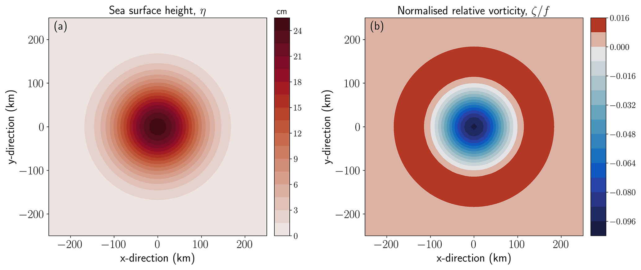
Figure 1 Idealised Gaussian eddy with anticyclonic rotation: (a) sea surface height (in cm), and (b) relative vorticity normalised by Coriolis parameter, f. Fields are calculated using the following parameters: A=25 cm, R=100 km, and $f={\mathrm{10}}^{-\mathrm{4}}$ s⁻¹.

2.1.2 Relative wind stress

Recall the bulk formula for relative wind stress in Eq. (2) given by

$$\begin{array}{}\text{(7)}& {\mathit{\tau }}_{\mathrm{rel}}={\mathit{\rho }}_{\mathrm{a}}{C}_{\mathrm{d}}|{\mathit{u}}_{\mathrm{a}}-{\mathit{u}}_{\mathrm{g}}|({\mathit{u}}_{\mathrm{a}}-{\mathit{u}}_{\mathrm{g}}),\end{array}$$

where only the geostrophic velocity component is employed to enable an analytical derivation. The drag coefficient C_d in Eq. (7) is set as a constant value to keep the analytical theory simple. The relative wind stress formula in Eq. (7) can be simplified by making use of the approximation due to Duhaut and Straub (2006) for the wind stress magnitude,

$$\begin{array}{}\text{(8)}& |{\mathit{u}}_{\mathrm{a}}-{\mathit{u}}_{\mathrm{g}}|\approx \left|{\mathit{u}}_{\mathrm{a}}\right|-{\mathit{u}}_{\mathrm{g}}\cdot \mathit{i},\end{array}$$

where i is a unit vector in the direction of the wind. This approximation is valid since we assume $\left|{\mathit{u}}_{\mathrm{a}}\right|\gg \left|{\mathit{u}}_{\mathrm{g}}\right|$. Equation (8) then tells us that only the ocean current aligned with the wind contributes significantly to the wind stress magnitude. A wind profile for u_a is chosen to be uniform in space, blowing zonally west to east, with zero meridional component, i.e. ${\mathit{u}}_{\mathrm{a}}=(u_{\mathrm{a}},\mathrm{0})$. This wind field represents a large-scale atmospheric wind with length scales larger than those of the mesoscale (Duhaut and Straub, 2006). The effect of the eddy current in relative wind stress is presented in Fig. 2a, which shows the difference in zonal wind stress, ${\mathit{\tau }}_{\mathrm{rel}}^x-{\mathit{\tau }}_{\mathrm{abs}}^x$. A dipole pattern of opposing values emerges at each meridional side of the eddy, where the largest values appear near the eddy radius.

2.1.3 Wind power input

The next step in deriving the analytical expression for relative wind stress damping is to find the work done by winds on the surface geostrophic motion. This is done by taking the dot product of relative wind stress and surface geostrophic velocities, and making use of Eq. (8):

$$\begin{array}{}\text{(9a)}& {\displaystyle }{W}_{\mathrm{rel}}& {\displaystyle }={\mathit{\tau }}_{\mathrm{rel}}\cdot {\mathit{u}}_{\mathrm{g}},\text{(9b)}& {\displaystyle }& {\displaystyle }={\mathit{\rho }}_{\mathrm{a}}{C}_{\mathrm{d}}|{\mathit{u}}_{\mathrm{a}}-{\mathit{u}}_{\mathrm{g}}|({\mathit{u}}_{\mathrm{a}}-{\mathit{u}}_{\mathrm{g}})\cdot {\mathit{u}}_{\mathrm{g}},\text{(9c)}& {\displaystyle }& {\displaystyle }={\mathit{\rho }}_{\mathrm{a}}{C}_{\mathrm{d}}\left(\right|u_{\mathrm{a}}|u_{\mathrm{a}}{u}_{\mathrm{g}}-|u_{\mathrm{a}}|u_{\mathrm{g}}^{\mathrm{2}}-u_{\mathrm{a}}{u}_{\mathrm{g}}^{\mathrm{2}}+u_{\mathrm{g}}^{\mathrm{3}}-|u_{\mathrm{a}}\left|v_{\mathrm{g}}^{\mathrm{2}}\right).\end{array}$$

First, we can see the effect of relative wind stress on wind work in Fig. 2b by plotting the difference between relative and absolute wind work (${\mathit{\tau }}_{\mathrm{rel}}\cdot {\mathit{u}}_{\mathrm{g}}-{\mathit{\tau }}_{\mathrm{abs}}\cdot {\mathit{u}}_{\mathrm{g}}$). Interpreting this wind work difference can be achieved by considering the values in Fig. 2a for an anticyclonic eddy (clockwise rotating). The negative wind stress difference in the north is multiplied by the positive anticyclonic eddy velocity, whilst the positive wind stress difference in the south is multiplied by the negative eddy velocity, and thus the wind work difference is negative everywhere. This shows wind work by relative wind stress is a net sink for a uniform large-scale wind. So we expect an analytical expression for relative wind stress damping to be negative sign-definite. We recognise that other wind profiles could exist, though these have not been explored in this current work.

To find the analytical expression, we put analytical equations for geostrophic velocities Eq. (6) into Eq. (9c) and integrate over horizontal space in the limits of $x,y\to \pm \mathrm{\infty }$:

$$\begin{array}{}\text{(10)}& P_{\mathrm{rel}}=\underset{-\mathrm{\infty }}{\overset{\mathrm{\infty }}{\int }}\underset{-\mathrm{\infty }}{\overset{\mathrm{\infty }}{\int }}{W}_{\mathrm{rel}}\mathrm{d}x\mathrm{d}y,\end{array}$$

which gives

$$\begin{array}{}\text{(11)}& P_{\mathrm{rel}}=-\mathrm{3}{\mathit{\rho }}_{\mathrm{a}}{C}_{\mathrm{d}}\left|u_{\mathrm{a}}\right|{\displaystyle \frac{g^{\mathrm{2}}{A}^{\mathrm{2}}\mathit{\pi }}{\mathrm{2}{f}^{\mathrm{2}}}},\end{array}$$

where P_rel has units kg m² s⁻³. The analytical equation for relative wind stress damping found in Eq. (11) is analogous to forms suggested by Gaube et al. (2015) and Jullien et al. (2020), although neither carried out a spatial integration. A few things can be inferred from Eq. (11) on P_rel. First, P_rel depends on the magnitude of the wind velocity, u_a, meaning that damping is independent of the wind direction. Second, P_rel is also independent of eddy polarity (sign of A) due to its quadratic dependence, implying that anticyclonic or cyclonic eddies will undergo equivalent damping when A is the same in absolute terms. We also see that P_rel does not depend on the eddy e-folding radius, R. This is because R cancels out in the integral limits of ±∞ for this circular eddy. Finally, with all this in mind, P_rel is always negative, informing that relative wind stress will damp eddy energy. If wind power input were to be calculated using absolute wind stress in Eq. (3), its spatial integral would equal zero (P_abs=0). Overall, this analytical finding is consistent with previous studies (Zhai and Greatbatch, 2007; Xu et al., 2016; Renault et al., 2016b; Rai et al., 2021) that find relative wind stress acts as a net sink of eddy energy.

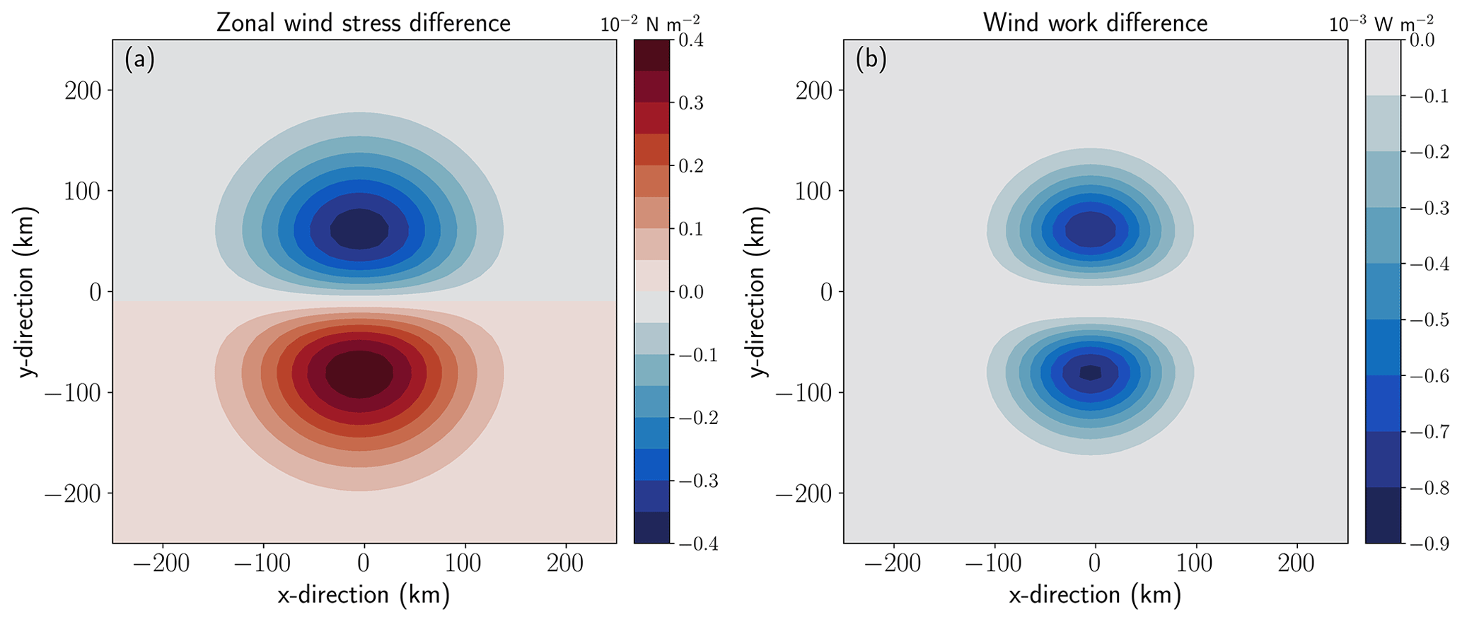
Figure 2 Horizontal views showing differences between relative and absolute wind stress calculated over an idealised Gaussian anticyclonic eddy: (a) difference in zonal wind stress, ${\mathit{\tau }}_{\mathrm{rel}}^x-{\mathit{\tau }}_{\mathrm{abs}}^x$ (in units 10⁻² N m⁻²), and (b) difference in wind work, W_rel−W_abs (in units 10⁻³ W m⁻²). Fields are calculated using the following parameters: A=25 cm, R=100 km, $f={\mathrm{10}}^{-\mathrm{4}}$ s⁻¹, u_a=7 m s⁻¹, $C_{\mathrm{d}}=\mathrm{1.1}\times {\mathrm{10}}^{-\mathrm{3}}$, and ρ_a=1.2 kg m⁻³. Relative wind stress is computed using the full expression in Eq. (7).

2.2 Describing an analytical eddy

Mesoscale ocean eddies take on a complex vertical structure, making them hard to accurately model. However, studies such as the one by Wunsch (1997) allow us to make a reasonable choice in choosing a simple eddy model. An alternative choice could be made by using surface modes (de La Lama et al., 2016; LaCasce, 2017), though we discuss these in more detail in Sect. 6. Wunsch (1997) detailed the variability in eddy kinetic energy (EKE) in the vertical, and found EKE to exist primarily in the barotropic and first baroclinic modes. These modes can be thought of in terms of their horizontal flow: the barotropic mode has flow that is completely depth independent; and the first baroclinic mode has flow that is depth dependent with a zero crossing at depth and zero net vertically integrated flow. Over the global ocean, Wunsch (1997) showed the first baroclinic mode contains the majority of EKE (60 %–70 %), though in some regions, such as south of the Gulf Stream, strong barotropic mode signals were found. Nevertheless, links with the eddy sea surface height and their vertical structure have further been made. It is now widely known that variations in eddy sea surface height reflect changes in the ocean's thermocline displacement, and thus changes in first baroclinic mode eddy energy (Smith and Vallis, 2001). In this work, we proceed, for simplicity, by representing an eddy using only the first baroclinic mode.

2.2.1 Baroclinic eddy

Two-layer shallow water equations are used to describe the baroclinic eddy:

$$\begin{array}{}\text{(12a)}& {\displaystyle }& {\displaystyle \frac{D{\mathit{u}}_{g\mathrm{1}}}{Dt}}+f\mathit{k}\times {\mathit{u}}_{g\mathrm{1}}=-g{\mathrm{\nabla }}_h\left({\mathit{\eta }}_{\mathrm{1}}\right)+{\displaystyle \frac{\mathit{\tau }}{{\mathit{\rho }}_{\mathrm{0}}{h}_{\mathrm{1}}}},\text{(12b)}& {\displaystyle }& {\displaystyle \frac{D{\mathit{u}}_{g\mathrm{2}}}{Dt}}+f\mathit{k}\times {\mathit{u}}_{g\mathrm{2}}=-g{\mathrm{\nabla }}_h\left({\mathit{\eta }}_{\mathrm{1}}\right)-g^{\prime }{\mathrm{\nabla }}_h\left({\mathit{\eta }}_{\mathrm{2}}\right),\text{(12c)}& {\displaystyle }& {\displaystyle \frac{\partial h_{\mathrm{1}}}{\partial t}}+{\mathrm{\nabla }}_h\cdot \left(h_{\mathrm{1}}{\mathit{u}}_{g\mathrm{1}}\right)=\mathrm{0},\text{(12d)}& {\displaystyle }& {\displaystyle \frac{\partial h_{\mathrm{2}}}{\partial t}}+{\mathrm{\nabla }}_h\cdot \left(h_{\mathrm{2}}{\mathit{u}}_{g\mathrm{2}}\right)=\mathrm{0},\end{array}$$

where ${\cdot }_{\mathrm{1},\mathrm{2}}$ denotes the upper and lower layer variables; η₂ is the interface displacement between the two layers, which is measured positive upwards; $g^{\prime }=g({\mathit{\rho }}_{\mathrm{2}}-{\mathit{\rho }}_{\mathrm{1}})/{\mathit{\rho }}_{\mathrm{2}}$ is the reduced gravity (the change in acceleration of gravity due to buoyant forces) found using upper and lower layer density; and $h_{\mathrm{1}}=H_{\mathrm{1}}+{\mathit{\eta }}_{\mathrm{1}}-{\mathit{\eta }}_{\mathrm{2}}$ and $h_{\mathrm{2}}=H_{\mathrm{2}}+{\mathit{\eta }}_{\mathrm{2}}$ are the respective layer depths of which H_1,2 is the reference layer depth. This two-layer model includes the effects of stratification through g^′, which accounts for the adjustment between the two layers due to the change in density. Equations (12a) and (12b) are momentum equations and Eqs. (12c) and (12d) are continuity equations. The second term on the right side of Eq. (12a) is the wind forcing.

Before progressing with the derivation of the baroclinic eddy energy equation, some points are discussed first. The two-layer shallow water equations in the form shown in Eq. (12) do not immediately describe the baroclinic eddy, but rather an ocean with two layers of differing density. It is known that the sea surface height typically reflects the displacement of the main thermocline (Wunsch, 1997). In this case, there exists proportionality between the upper and lower layers in the two-layer analytical model, and as such the vertical structure of the baroclinic eddy can be described. Following Cushman-Roisin and Beckers (2006), η₁=μη₂ and u₂=λu₁, where μ and λ are proportionality coefficients to be defined, which both provide the dynamical structure of the eddy through normal modes. Normal modes exhibit wave patterns that depend on these proportionality coefficients, and these are found as follows: equating together the momentum Eqs. (12b) with (12a) and neglecting wind stress gives

$$\begin{array}{}\text{(13)}& \mathit{\lambda }={\displaystyle \frac{g\mathit{\mu }+g^{\prime }}{g\mathit{\mu }}},\end{array}$$

and then equating the continuity Eq. (12d) with (12c) gives

$$\begin{array}{}\text{(14)}& {\displaystyle \frac{\mathrm{1}}{\mathit{\mu }-\mathrm{1}}}={\displaystyle \frac{H_{\mathrm{2}}\mathit{\lambda }}{H_{\mathrm{1}}}}.\end{array}$$

A quadratic equation for λ can be found from Eqs. (13) and (14):

$$\begin{array}{}\text{(15)}& H_{\mathrm{2}}{\mathit{\lambda }}^{\mathrm{2}}+(H_{\mathrm{1}}-H_{\mathrm{2}})\mathit{\lambda }-H_{\mathrm{1}}=\mathrm{0}.\end{array}$$

In Eq. (15), there are two solutions for λ that relate to the barotropic (BT) and first baroclinic mode (BC1). In the limit $g^{\prime }/g\to \mathrm{0}$, the BT is described by λ=1 and $\mathit{\mu }=H/H_{\mathrm{2}}$, and BC1 is given by $\mathit{\lambda }=-H_{\mathrm{1}}/H_{\mathrm{2}}$ and $\mathit{\mu }=-g^{\prime }{H}_{\mathrm{2}}/gH$. A baroclinic eddy is therefore represented by the two-layer model through the use of BC1's λ and μ. Whilst H₁ is the depth of the upper layer, in BC1 this can also be defined as the first baroclinic mode zero crossing. An example of this mode can be seen in Fig. 1 of Wunsch (1997).

2.2.2 Eddy energy equation

The derivation of the two-layer energy equation is done as follows: Equation (12a) is multiplied by h₁u_g1, Eq. (12b) by h₂u_g2, Eq. (12c) by gη₁, and Eq. (12d) by g^′η₂, giving the upper and lower layer kinetic and potential energy equations, respectively. The resulting equations are added together to give the total eddy energy equation for an analytical baroclinic eddy:

$$\begin{array}{}\text{(16)}& \begin{array}{rl}& {\displaystyle \frac{\partial }{\partial t}}\left({\mathit{\rho }}_{\mathrm{0}}\left(h_{\mathrm{1}}{\displaystyle \frac{\mathrm{1}}{\mathrm{2}}}{\mathit{u}}_{g\mathrm{1}}\cdot {\mathit{u}}_{g\mathrm{1}}+h_{\mathrm{2}}{\displaystyle \frac{\mathrm{1}}{\mathrm{2}}}{\mathit{u}}_{g\mathrm{2}}\cdot {\mathit{u}}_{g\mathrm{2}}+{\displaystyle \frac{\mathrm{1}}{\mathrm{2}}}g{\mathit{\eta }}_{\mathrm{1}}^{\mathrm{2}}\right.\right.\\ & \left.\left.+{\displaystyle \frac{\mathrm{1}}{\mathrm{2}}}g\prime {\mathit{\eta }}_{\mathrm{2}}^{\mathrm{2}}\right)\right)+{\mathrm{\nabla }}_h\cdot \left({\mathit{\rho }}_{\mathrm{0}}\left({\displaystyle \frac{\mathrm{1}}{\mathrm{2}}}{\mathit{u}}_{g\mathrm{1}}\cdot {\mathit{u}}_{g\mathrm{1}}+g{\mathit{\eta }}_{\mathrm{1}}\right)h_{\mathrm{1}}{\mathit{u}}_{g\mathrm{1}}\right.\\ & \left.+{\mathit{\rho }}_{\mathrm{0}}\left({\displaystyle \frac{\mathrm{1}}{\mathrm{2}}}{\mathit{u}}_{g\mathrm{2}}\cdot {\mathit{u}}_{g\mathrm{2}}+g{\mathit{\eta }}_{\mathrm{1}}+g\prime {\mathit{\eta }}_{\mathrm{2}}\right)h_{\mathrm{2}}{\mathit{u}}_{g\mathrm{2}}\right)\\ & =\mathit{\tau }\cdot {\mathit{u}}_{g\mathrm{1}}.\end{array}\end{array}$$

In Eq. (16), terms in the top row in the order of left to right are upper layer kinetic energy, lower layer kinetic energy, upper layer potential energy, and lower layer potential energy. Terms in the middle represent the divergence of kinetic and potential energy, as well as divergence of pressure work. In the bottom row is the work done by winds on the surface geostrophic motion.

We now want to acquire an analytical equation for Eq. (16) that we can use to approximate the damping of eddy energy by relative wind stress. To achieve this, Eq. (16) is integrated over space using analytical terms for η_1,2 and u_g1,2, where the upper layer terms are given in Eqs. (5) and (6), and the lower layer terms are found using the proportionality coefficients μ and λ. First, the combined kinetic and potential energy term from the top row of Eq. (16) leads to the following analytical form:

$$\begin{array}{}\text{(17)}& \begin{array}{rl}& (\mathrm{KE}+\mathrm{PE}{)}_{\mathrm{bc}}\equiv E={\mathit{\rho }}_{\mathrm{0}}\mathit{\pi }(\left(\right(H_{\mathrm{1}}-{\mathit{\lambda }}^{\mathrm{2}}{H}_{\mathrm{1}}+{\mathit{\lambda }}^{\mathrm{2}}H){\displaystyle \frac{g^{\mathrm{2}}}{\mathrm{2}{f}^{\mathrm{2}}}}\\ & +R^{\mathrm{2}}{\displaystyle \frac{g}{\mathrm{4}}}+R^{\mathrm{2}}{\displaystyle \frac{g\prime }{\mathrm{4}{\mathit{\mu }}^{\mathrm{2}}}})A^{\mathrm{2}}+\left((\mathrm{1}-{\displaystyle \frac{\mathrm{1}}{\mathit{\mu }}}+{\displaystyle \frac{{\mathit{\lambda }}^{\mathrm{2}}}{\mathit{\mu }}}){\displaystyle \frac{\mathrm{2}{g}^{\mathrm{2}}}{\mathrm{9}{f}^{\mathrm{2}}}}\right)A^{\mathrm{3}}).\end{array}\end{array}$$

This form is measured in units of kg m² s⁻². Of the two terms that contain R, the second one makes up the available potential energy from the lower layer. Since the terms in the middle row of Eq. (16) represent the divergence of energy flux in the domain, under no normal flow boundary conditions is the integral of this term zero. Next, the integral of the first term in the bottom row of 16 is the wind power input, previously derived in Sect. 2.1.

After integrating Eq. (16), we arrive at an equation in the form

$$\begin{array}{}\text{(18)}& {\displaystyle \frac{\partial }{\partial t}}(\mathrm{KE}+\mathrm{PE}{)}_{\mathrm{bc}}=P,\end{array}$$

where (KE+PE)_bc is combined baroclinic kinetic and potential energy per unit volume, and P is wind power input. Equation (18) now depends on a few key eddy parameters, in particular eddy amplitude, A. For a geostrophic eddy, this means we can take its amplitude and infer the evolution of total eddy energy in response to relative wind stress damping. To do this, the energy Eq. (18) is integrated forward in time using a fourth-order Runge–Kutta scheme for the first two time steps ($n=\mathrm{2},\mathrm{3}$), followed by a third-order Adams–Bashforth scheme for time steps $n=\mathrm{4},\mathrm{\cdots }$. The Adams–Bashforth scheme is employed to match that used in the MITgcm. Once total eddy energy is found at the next time step n+1, eddy amplitude A is recovered from eddy energy E in Eq. (17) through a Newton–Raphson root finder method. The time evolution of analytical eddy energy is then compared with a numerical model in Sect. 4.

3 Experimental design

3.1 Numerical configuration

The numerical experiments were performed using the hydrostatic MIT general circulation model (Marshall et al., 1997a, b). Employing this numerical model is done so we can verify whether the analytical wind power input derived in Sect. 2.1 can sufficiently predict the decay of baroclinic eddy energy due to relative wind stress. The numerical setup was described in detail in Wilder et al. (2022), though we describe some pertinent details along with our attempt to design a continuously stratified model that displays similar characteristics to the analytical two-layer model.

The numerical model is set up on an f plane in a box-like domain spanning 2000 km in each x and y direction with equal grid spacing of 10 km. The ocean is 4000 m deep and the vertical grid has 91 z levels with spacing of 5 m at the surface and 100 m at depth. The ocean bottom is flat and a free-slip boundary condition is used, along with no bottom drag. Neglecting bottom drag may have repercussions for the cascade of eddy energy (Scott and Arbic, 2007); however, its neglect means damping by relative wind stress can be isolated in our model. A grid-scale biharmonic viscosity is used for numerical stability purposes as well as to parameterise the dissipation of energy at the smallest of scales.

The baroclinic eddy is initialised using analytical equations. The stratification is given by a 3D temperature field of the form

$$\begin{array}{}\text{(19)}& T(x,y,z)=T^{\prime }{e}^{-(x^{\mathrm{2}}+y^{\mathrm{2}})/R^{\mathrm{2}}}{e}^{-\mathit{\gamma }(z/H_{\mathrm{1}})}+T_{\mathrm{ref}}\left(z\right),\end{array}$$

where T^′ is the temperature anomaly, γ influences the stratification of the water column, z are vertical grid levels measured positive downward, and H₁ is the thermocline depth. The background temperature T_ref is derived using the linear equation of state from a reference background density given by

$$\begin{array}{}\text{(20)}& \begin{array}{rl}{\mathit{\rho }}_{\mathrm{ref}}\left(z\right)=& {\mathit{\rho }}_{\mathrm{0}}(\mathrm{1}-N_{\mathrm{0}}^{\mathrm{2}}z/g)+\mathrm{0.5}\mathrm{\Delta }\mathit{\rho }\\ & (\mathrm{1}-\tanh (B(z+H_{\mathrm{1}})/H\left)\right),\end{array}\end{array}$$

where ρ₀ is a reference density, N₀ is a reference buoyancy frequency, Δρ is the difference in density between the surface and bottom, B is the gradient of the density profile, and H is the depth of the ocean. Horizontal velocities are in thermal wind balance,

$$\begin{array}{}\text{(21)}& {\mathit{u}}_{\mathrm{g}}(x,y,z)={\displaystyle \frac{g}{f}}\mathit{k}\times \left(\mathrm{\nabla }\mathit{\eta }+\mathit{\alpha }\underset{z}{\overset{\mathrm{0}}{\int }}\mathrm{\nabla }T\mathrm{d}z\right),\end{array}$$

where ${\mathit{u}}_{\mathrm{g}}=(u_{\mathrm{g}},v_{\mathrm{g}})$ are zonal and meridional geostrophic velocity components, and α is the thermal expansion coefficient. In Eq. (21), the first term in the brackets is surface velocity derived from sea surface height, and the second term is vertical velocity shear derived from thermal wind balance.

So that an adequate comparison of the two-layer baroclinic eddy in Sect. 2.2.1 can be made with the stratified model described here, a few parameters in Eqs. (19) and (20) need to be tuned appropriately. In the two-layer model, the first baroclinic mode has zero net vertically integrated flow in the horizontal, where H₁ is the point where horizontal velocities are zero. This means that flow in the upper layer is countered by an opposing lower layer flow defined by

$$\begin{array}{}\text{(22)}& \underset{-H}{\overset{\mathrm{0}}{\int }}{\mathit{u}}_g\mathrm{d}z=\mathrm{0}.\end{array}$$

We minimise net flow in the stratified model by tuning parameters A, T^′, γ, and B. The aim is to achieve a minimal net flow and also have similar eddy properties between each setup, e.g. layer depths and sea surface height. We find the horizontal net flow in the MITgcm is close to zero. This implies the presence of a barotropic mode component in this setup, which is not too dissimilar to the real ocean (Wunsch, 1997; Arbic and Flierl, 2004). Some key model parameters are shown in Table 1.

The wind field used in this setup is uniform in one direction and is designed to represent a large-scale background wind. (See Wilder et al. (2022) for further details on the wind setup.) The drag coefficient in the wind stress formula is a function of the magnitude of the wind speed (Large and Pond, 1981), which is different from the analytical model where C_d is constant. However, the differences in drag coefficient are not expected to cause large differences between the total wind damping in the numerical and analytical models (Wilder, 2022).

When the model is first initialised it is allowed to run for 10 d with zero wind forcing. This allows any inertial waves to die down and also lets the equations of motion form a balance that could be slightly different from that of geostrophy. After this adjustment phase, the wind forcing is turned on and the model is run for 400 d.

Table 1 Key experimental parameters.

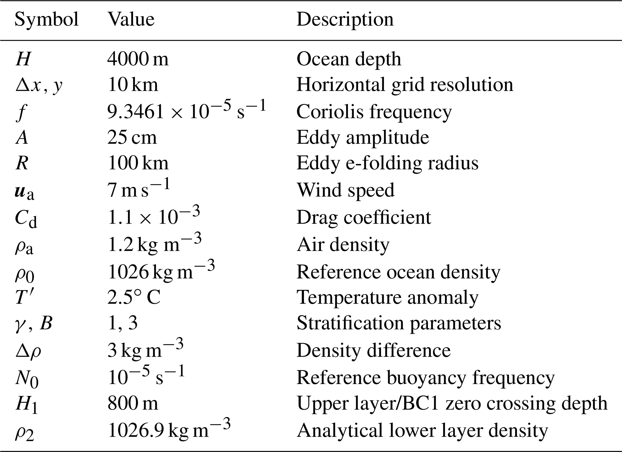
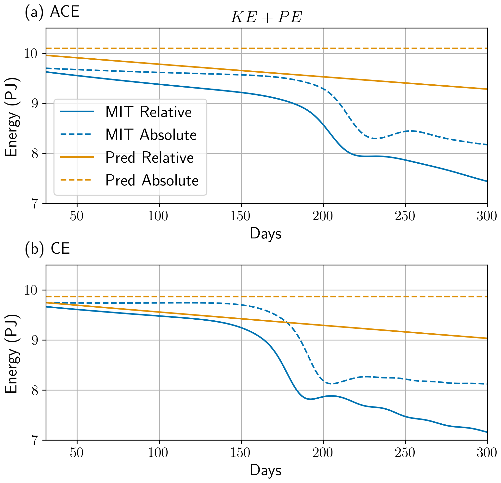
Figure 3 Time series of total eddy energy, E, for (a) anticyclone and (b) cyclone. MITgcm is given by either MIT Relative or MIT Absolute, and the analytical model is given by either Pred Relative or Pred Absolute. Units of energy are in PJ. MITgcm values are 16 d time means.

3.2 Diagnosing model energetics

To validate the evolution of baroclinic eddy energy in the analytical model (Sect. 2.2.1), time-mean quantities of kinetic and potential energy, and wind damping for the continuously stratified MITgcm model, need to be defined. The following are mean potential energy, mean kinetic energy, and wind power input:

$$\begin{array}{}\text{(23)}& {\displaystyle }\mathrm{PE}& {\displaystyle }=-\underset{V}{\int }{\displaystyle \frac{g}{\mathrm{2}{n}_{\mathrm{0}}\left(z\right)}}{\stackrel{\mathrm{‾}}{{\mathit{\rho }}^{*}(x,y,z,t)}}^{\mathrm{2}}\mathrm{d}V,\text{(24)}& {\displaystyle }\mathrm{KE}& {\displaystyle }=\underset{V}{\int }{\displaystyle \frac{{\mathit{\rho }}_{\mathrm{0}}}{\mathrm{2}}}({\stackrel{\mathrm{‾}}{u}}_{\mathrm{g}}^{\mathrm{2}}+{\stackrel{\mathrm{‾}}{v}}_g^{\mathrm{2}})\mathrm{d}V,\text{(25)}& {\displaystyle }P& {\displaystyle }=\underset{S}{\int }\stackrel{\mathrm{‾}}{\mathit{\tau }}\cdot {\stackrel{\mathrm{‾}}{\mathit{u}}}_{\mathrm{g}}\mathrm{d}S,\end{array}$$

where $\stackrel{\mathrm{‾}}{\cdot }$ represents a 16 d time mean, ${\mathit{\rho }}^{*}(x,y,z,t)=\mathit{\rho }(x,y,z,t)-{\mathit{\rho }}_{\mathrm{ref}}\left(z\right)$ is a density anomaly relative to a constant-in-time reference background density state, n₀(z) is the vertical gradient of ρ_ref(z), u_g and v_g are geostrophic velocity components in the zonal and meridional direction, and ∫_V is a volume integral. The density field $\mathit{\rho }(x,y,z,t)$ is computed from the MITgcm temperature field, and ρ_ref(z) is given in Eq. (20). Use of the potential energy anomaly informs how much potential energy can be converted into kinetic energy, as opposed to how much potential energy exists within the stratification. Choosing the potential energy definition in Eq. (23) implies a quasi-geostrophic framework and has been used in past studies (von Storch et al., 2012; Chen et al., 2014; Youngs et al., 2017).

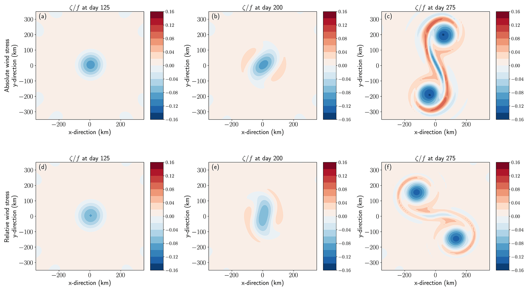
Figure 4 Horizontal views of MITgcm surface geostrophic relative vorticity normalised by Coriolis frequency in an anticyclonic eddy for absolute (top) and relative (bottom) wind stress at days (a, d) 125, (b, e) 200, and (c, f) 275. Fields are calculated using daily mean SSH output from MITgcm simulations.

3.3 Setting up the analytical model

The time evolution of analytical eddy energy is achieved by time-stepping Eq. (18) forward in time. To begin the time-stepping of the analytical model, initial eddy energy and dissipation is found by using data from the MITgcm model run, such as eddy amplitude. Equivalent eddy energy is desired to visualise the rate of decay imposed by relative wind stress. Because the MITgcm setup has been chosen to display similar characteristics to the analytical model, the energetics are thus fixed. To make eddy energy in the analytical model match the MITgcm setup, we modify the analytical lower layer density until potential energy matches (see Table 1). Kinetic energy is only a small fraction of total eddy energy, so there is less importance in matching this quantity between the analytical and numerical setups. Overall, these details allow us to make a consistent comparison between both setups and examine more clearly the rate of eddy energy decay by relative wind stress.

4 Verifying the analytical model

In this section we present our first set of results, comparing the time evolution of the analytical and numerical eddy energy budgets. Figure 3 shows a time series of domain-integrated eddy energy (KE + PE) for an anticyclonic (ACE) and cyclonic (CE) eddy. The first thing that can be seen is the initial offset in total eddy energy between the analytical model (Pred) and the numerical model (MIT) in ACE and CE. Here, potential energy is being matched between the analytical and numerical models, and therefore the discrepancy implies that the kinetic energy contribution is not equivalent between Pred and MIT. This kinetic energy mismatch is expected since the two-layer analytical eddy cannot realistically represent the continuously stratified MITgcm eddy.

We first focus on the first 150 d of the ACE (Fig. 3a). In the absolute wind stress case (AW), AW MIT is damped by 0.1 PJ up to day 150, while AW Pred sees zero energy loss due to absolute wind stress not damping the eddy. In the relative wind stress case (RW), the negative wind power input (Fig. 5a) is able to remove eddy energy from RW Pred and RW MIT. Up to day 150, RW Pred loses 0.38 PJ whilst RW MIT loses around 0.4 PJ, relative to day 31 in the RW time series. This damping by relative wind stress is similar because the wind power input in Pred and MIT is around $-\mathrm{3}\times {\mathrm{10}}^{\mathrm{7}}$ W.

Beyond day 150, Pred and MIT time series begin to diverge, with MIT undergoing a sudden reduction in total energy of around 10 % over 30 d, whilst Pred continues with a smooth decay. This divergence indicates that MIT is no longer evolving as it initially did, suggesting the eddy is undergoing an instability process and departing from its initial state. In RW, this sudden reduction in total energy also takes place at an earlier timescale. These possible instabilities may also impact the relative wind power input, since P_rel displays a sharp increase in negative wind power input (Fig. 5). (An in-depth examination of the anticyclonic eddy response can be found in Wilder et al. (2022), and therefore the finer details are omitted from this discussion.) From day 250, the rate of decay in MIT slows for each wind stress and is much more closely aligned with the decay rate in Pred. Inspecting the ACE eddy surface relative vorticity in Fig. 4 illustrates the regime change of the eddy, consistent with the changes seen in the time series (Fig. 3). The ACE under AW and RW is initially coherent at day 125 (Fig. 4a, d), then develops two outer lobes of stronger cyclonic vorticity by day 200 (Fig. 4b, e), before eventually splitting into two separate anticyclonic eddies by day 275 (Fig. 4c, f). This process of eddy splitting in baroclinic eddies has been well documented in previous studies (Ikeda, 1981; Dewar et al., 1999), where timescales vary with the parameter values chosen (Mahdinia et al., 2017).

Similar results are also observed for the CE (Fig. 3b). The decay rate in total energy follows roughly the same trajectory as the ACE up to 150 d, with more damping taking place in RW Pred and RW MIT due to negative wind power input (Fig. 5b). As discussed earlier, wind power input due to relative wind stress is independent of eddy polarity, so no bias in damping rate should exist. Up to day 130 of the time series, RW Pred is damped by 0.37 PJ and RW MIT is damped by 0.26 PJ. The disparity in damping is not a result of unequal dissipation rates by P_rel (Fig. 5b) but is a result of energy production in MIT via vertical diffusive processes. Indeed, running a simulation with no eddy and no wind, but with vertical diffusion, did result in potential energy production (not shown). However, why this is more prominent in the cyclonic eddy than in the anticyclonic eddy has not been investigated further. After day 150, MIT exhibits a sudden reduction in total energy with each wind stress, which happens earlier in RW. Moreover, in contrast to the ACE, the timescale for this sudden reduction to take place in the CE is around 15 %–20 % shorter. This points to an anticyclone–cyclone asymmetry, which has been recognised in past studies (Chelton et al., 2011; Mkhinini et al., 2014; Mahdinia et al., 2017).

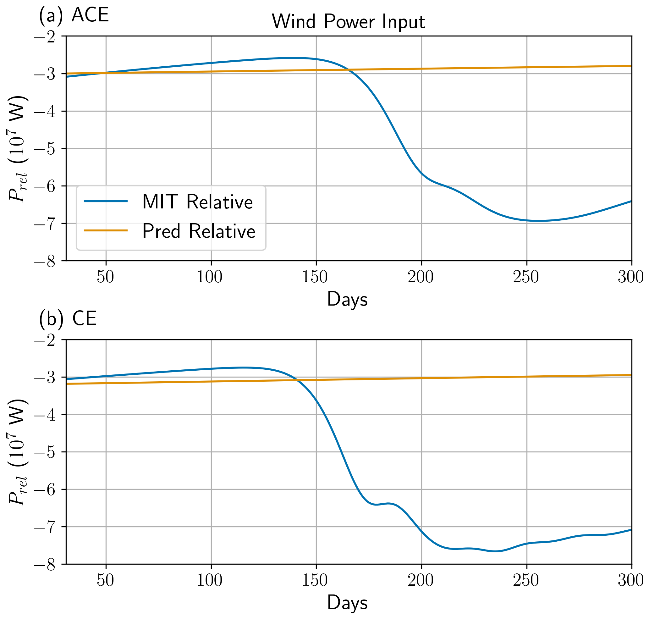
Figure 5 Time series of total wind power input in relative wind stress simulation, P_rel, for (a) anticyclone and (b) cyclone. MITgcm is given by MIT Relative and the analytical model is given by Pred Relative. Units of power are in W. MITgcm values are 16 d time means.

In this section we have compared the evolution of total eddy energy between an analytical and a numerical model. The results tell us that a two-layer analytical model can reasonably explain the evolution of total eddy energy in the MIT simulation. However, the agreement between both models diminishes due to an instability process in the MIT simulation. Nevertheless, we find the timescale of around ∼150 d for eddy energy agreement to be acceptable and, as such, feel confident to propose a constrained eddy energy dissipation rate in Sect. 5.

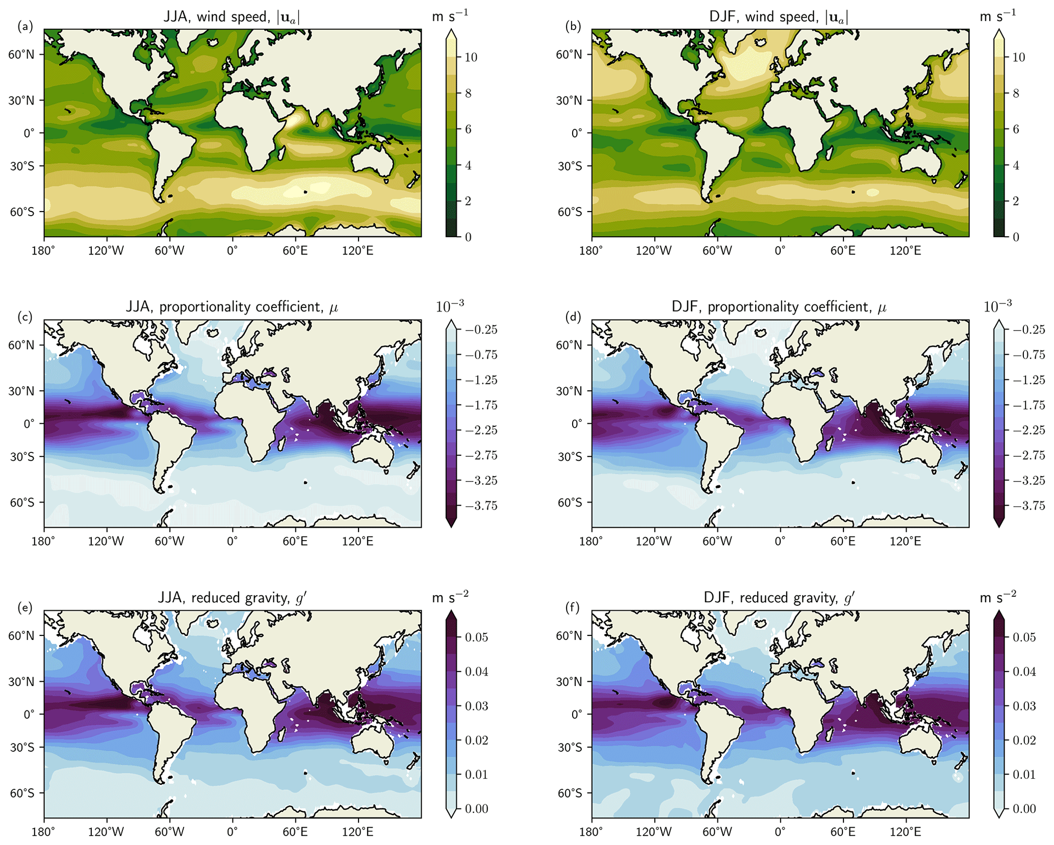
Figure 6 Global maps between the latitudes of 70^∘ S and 70^∘ N displaying contributions to the dissipation rate, Λ_rel, for (a, c, e) June–July–August (JJA) and (b, d, f) December–January–February (DJF). Panels (a, b) show wind speed, $\left|{\mathit{u}}_{\mathrm{a}}\right|$ (in m s⁻¹), (c, d) proportionality coefficient, μ, and (e, f) reduced gravity, g^′ (in m s⁻²). The data are calculated from World Ocean Atlas and NOAA datasets over the period 1981–2010.

5 A constrained dissipation rate

An eddy energy dissipation rate due to relative wind stress takes the form

$$\begin{array}{}\text{(26)}& {\mathrm{\Lambda }}_{\mathrm{rel}}=\left|P_{\mathrm{rel}}\right|/E,\end{array}$$

and it can be found by putting the analytical equations for P_rel from Eq. (11) and E from Eq. (17) into the above equation for a constrained Λ_rel. Since the analytical eddy energy E is made up of several terms, we will simplify E by finding its dominant term. A simple scaling of Eq. (17) shows potential energy within the thermocline to be the dominant term. For this we choose typical parameter values: H=4000 m, H₁=800 m, ρ₁=1026 kg m⁻³, ρ₂=1029 kg m⁻³, R=100 km, and $f={\mathrm{10}}^{-\mathrm{4}}$ s⁻¹. Putting these values into Eq. (17) gives an approximation to eddy energy as

$$\begin{array}{}\text{(27)}& E\approx {\mathit{\rho }}_{\mathrm{0}}\mathit{\pi }{\displaystyle \frac{R^{\mathrm{2}}g\prime A^{\mathrm{2}}}{\mathrm{4}{\mathit{\mu }}^{\mathrm{2}}}}.\end{array}$$

Moreover, it is also well known that potential energy is greater than kinetic energy when the scale of motions exceed the first baroclinic radius of deformation (Gill et al., 1974). As such, mesoscale eddies will have potential energy much greater than kinetic energy. Furthermore, for this dissipation rate to be formed of potential energy, we are also arguing that relative wind stress has an immediate effect on the dissipation of potential energy, and there are no delays in the timescale of this communication. While relative wind stress directly damps eddy surface motions, Wilder et al. (2022) show that relative wind stress simultaneously releases potential energy via wind-induced baroclinic conversion. Therefore, the dissipation rate of eddy energy in Eq. (27) due to relative wind stress in Eq. (11) can take the form

$$\begin{array}{}\text{(28)}& {\mathrm{\Lambda }}_{\mathrm{rel}}\approx {\displaystyle \frac{\mathrm{6}{\mathit{\rho }}_{\mathrm{a}}{C}_{\mathrm{d}}\left|u_{\mathrm{a}}\right|g^{\mathrm{2}}{\mathit{\mu }}^{\mathrm{2}}}{{\mathit{\rho }}_{\mathrm{0}}{R}^{\mathrm{2}}{g}^{\prime }{f}^{\mathrm{2}}}}.\end{array}$$

The dissipation rate Λ_rel is independent of eddy amplitude due to P_rel and E being functions of A². We see instead that Λ_rel depends on a few terms that can vary in space, such as the magnitude of wind velocity $\left|u_{\mathrm{a}}\right|$, proportionality coefficient μ, eddy length scale R, and reduced gravity g^′. It is worth pointing out that in the limit of $H_{\mathrm{1}}/H_{\mathrm{2}}\to \mathrm{0}$ and $\mathit{\mu }\to g^{\prime }/g$, such as in the 1.5-layer model (Vallis, 2017), Eq. 28 further simplifies to

$$\begin{array}{}\text{(29)}& {\mathrm{\Lambda }}_{\mathrm{rel}}\approx {\displaystyle \frac{\mathrm{6}{\mathit{\rho }}_{\mathrm{a}}{C}_{\mathrm{d}}\left|u_{\mathrm{a}}\right|g^{\prime }}{{\mathit{\rho }}_{\mathrm{0}}{R}^{\mathrm{2}}{f}^{\mathrm{2}}}},\end{array}$$

which clearly shows the importance of g^′ for determining the dissipation rate. We proceed with Eq. (28) throughout Sect. 5. In addition, we now consider eddies to be deviations from the time mean, rather than just being a singular coherent eddy. The interpretation of the dissipation rate can also be thought of as one for these eddy time-mean deviations.

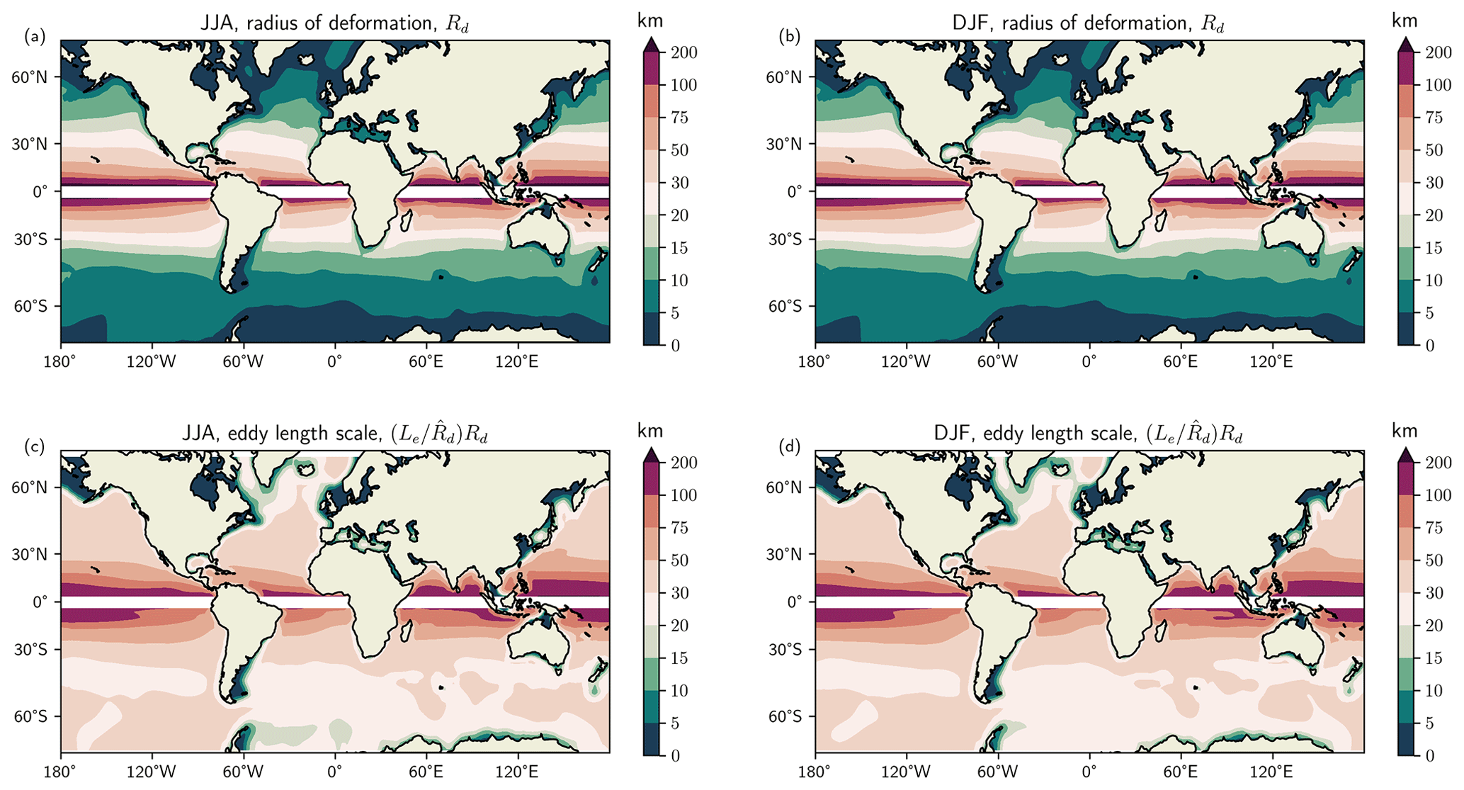
Figure 7 Global maps between the latitudes of 70^∘ S and 70^∘ N displaying the eddy length scale (in kilometres) for (a, c) JJA and (b, d) DJF. Panels (a, b) show the first baroclinic Rossby radius of deformation, R_d. Panels (c, d) show the eddy e-folding length scale, $(L_{\mathrm{e}}/{\widehat{R}}_{\mathrm{d}})R_{\mathrm{d}}$. The R_d is calculated from World Ocean Atlas and NOAA datasets over the period 1981–2010, and $(L_{\mathrm{e}}/{\widehat{R}}_{\mathrm{d}})R_{\mathrm{d}}$ is computed using data from Chelton et al. (2011). A latitude band between 5^∘ S and 5^∘ N has been masked out. The colourbar has uneven intervals, with spacing increasing with length scale.

5.1 Calculating the dissipation rate

We approach the computation of the dissipation rate Λ_rel in Eq. (28) by acquiring datasets for $\left|{\mathit{u}}_{\mathrm{a}}\right|$, μ, R, and g^′. Wind data are now assumed to be the wind speed $\left|{\mathit{u}}_{\mathrm{a}}\right|$, rather than just the zonal wind velocity component $\left|u_{\mathrm{a}}\right|$, because wind patterns vary in latitude and longitude over the global ocean. Wind speed is taken from the NCEP–NCAR Reanalysis 1 data (Kalnay et al., 1996) and is on a 2 degree horizontal grid. The wind speed data are then interpolated onto a 1 degree horizontal grid. The remaining terms require temperature and salinity datasets, and these are taken from the World Ocean Atlas (Locarnini et al., 2019; Zweng et al., 2019) on a 1 degree horizontal grid. Each dataset is made up of long-term monthly means over the period 1981–2010, which are averaged into seasons June–July–August (JJA) and December–January–February (DJF). The terms μ and g^′ are found by solving a Sturm–Liouville eigenvalue problem for the first baroclinic mode using the temperature and salinity fields (see Sect. 5.1.1). Arriving at an approximation for the eddy length scale R comes with some uncertainty, and for this reason we establish two forms for R. As a result, we will also form two choices for the dissipation rate that will indicate between where we might expect the value to fall. From the eigenvalue problem (Sect. 5.1.1), the first baroclinic Rossby radius of deformation, R_d, can be found, which we take as one choice for R. Another choice for R is found by scaling our computed R_d with data from Chelton et al. (2011), Fig. 12, where an e-folding radius L_e, and Rossby radius ${\widehat{R}}_{\mathrm{d}}$, are presented over latitude as zonal averages. That is, our values of R are given as either R_d or $(L_{\mathrm{e}}/{\widehat{R}}_{\mathrm{d}})R_{\mathrm{d}}$.

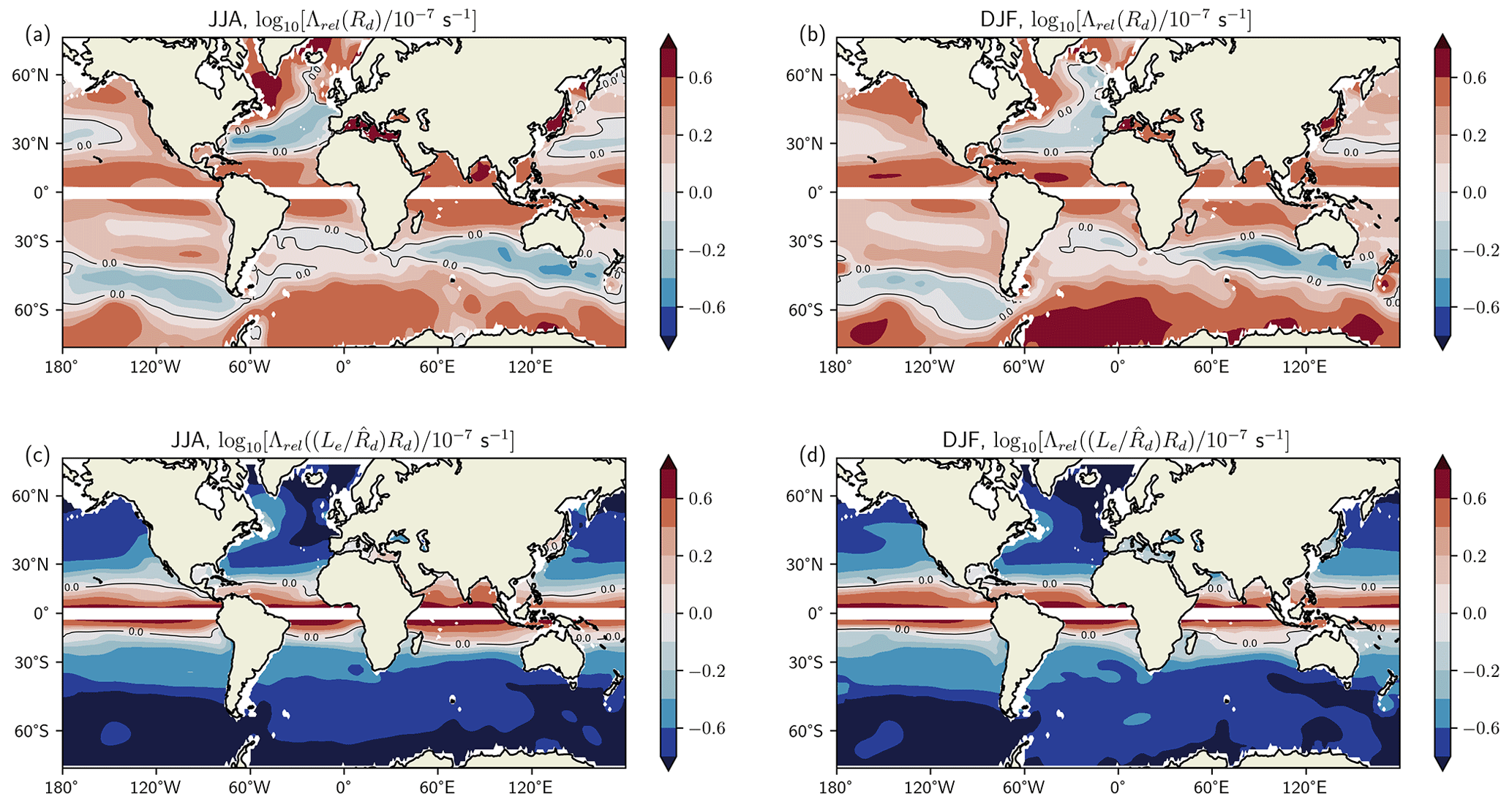
Figure 8 A global dissipation rate for relative wind stress damping, Λ_rel, for (a, c) JJA and (b, d) DJF. In (a, b) Λ_rel is a function of R_d, and in (c, d) Λ_rel is a function of $(L_{\mathrm{e}}/{\widehat{R}}_{\mathrm{d}})R_{\mathrm{d}}$. The dissipation rate is normalised by a constant dissipation rate, 10⁻⁷ s⁻¹, used in Mak et al. (2018). It is then shown on a log ₁₀ plot. The colourbar has uneven intervals, with smaller steps around zero to highlight when both dissipation rates are equivalent, or Λ_rel is marginally less than or greater than 10⁻⁷ s⁻¹. The thick contour line represents the point where ${\mathrm{\Lambda }}_{\mathrm{rel}}={\mathrm{10}}^{-\mathrm{7}}$ s⁻¹. A latitude band between 5^∘ S and 5^∘ N has been masked out.

5.1.1 The eigenvalue problem

Following Xu et al. (2011), the eigenvalue problem takes the form

$$\begin{array}{}\text{(30)}& {\displaystyle \frac{\mathrm{d}}{\mathrm{d}z}}\left({\displaystyle \frac{f^{\mathrm{2}}}{N^{\mathrm{2}}}}{\displaystyle \frac{\mathrm{d}{\mathit{\varphi }}_n\left(z\right)}{\mathrm{d}z}}\right)+{\mathit{\lambda }}_n{\mathit{\varphi }}_n\left(z\right)=\mathrm{0},\end{array}$$

with boundary conditions

$$\begin{array}{}\text{(31)}& \left({\displaystyle \frac{\mathrm{1}}{N^{\mathrm{2}}}}\right){\displaystyle \frac{\mathrm{d}\mathit{\varphi }}{\mathrm{d}z}}=\mathrm{0}\text{at}z=\mathrm{0},-H,\end{array}$$

where ϕ_n(z) is the eigenmode, λ_n is the eigenvalue, $N\left(z\right)=-(g/{\mathit{\rho }}_{\mathrm{0}})\partial {\mathit{\rho }}^{\prime }(x,y,z)/\partial z$ is the buoyancy frequency, and ${\mathit{\rho }}^{\prime }(x,y,z)$ is a density anomaly with respect to a reference ocean density, ρ₀. Here, λ_n is not the same as λ defined in Sect. 2.2.1, and H is the depth of the ocean taken from the World Ocean Atlas datasets, not the value given in Table 1, and therefore varies in space. The subscript ⋅_n is the nth mode. The Gibbs SeaWater Oceanographic Toolbox (McDougall and Barker, 2011) is used to calculate ρ. The eigenvalue problem Eq. (30) is solved using the MATLAB function dynmodes.m (Klinck, 2009), and locations where the ocean depth is shallower than 300 m are not considered. From Flierl (1978), the first baroclinic Rossby radius of deformation is related to the eigenvalue by $R_{\mathrm{d}}=\mathrm{1}/\sqrt{{\mathit{\lambda }}_{\mathrm{1}}}$. We subsequently use R_d as one of our choices for the length scale of mesoscale eddies. We take the depth of zero crossing of the first baroclinic mode to be H₁. The eigenmode is normalised using

$$\begin{array}{}\text{(32)}& \underset{-H}{\overset{\mathrm{0}}{\int }}{\mathit{\varphi }}_i{\mathit{\varphi }}_j\mathrm{d}z=H{\mathit{\delta }}_{ij}.\end{array}$$

Reduced gravity is defined by Xu et al. (2011) as $g^{\prime }=f^{\mathrm{2}}(\mathrm{1}+{\mathit{\varphi }}_{\mathrm{1}}^{\mathrm{2}}(\mathrm{0}\left)\right)/{\mathit{\lambda }}_{\mathrm{1}}{H}_{\mathrm{2}}$. The coefficient μ is defined as previously in Sect. 2.2.1 and is quantified by using the calculated terms g^′ and H₁.

5.1.2 The contributing terms

Figure 6 displays the terms $\left|{\mathit{u}}_{\mathrm{a}}\right|$, μ, and g^′ over the global ocean. Figure 6a and b illustrate the wide variability in space and time for the wind speed. There is a clear increase in $\left|{\mathit{u}}_{\mathrm{a}}\right|$ at higher latitudes during each hemispheric winter, while there is a slow down in winds during their summer. The largest wind speeds occur around 90^∘ E in the Southern Ocean, whilst the western boundaries see values a few metres per second lower. In the μ term, there is a slight variation between seasons, with the largest absolute values over the equatorial regions (Fig. 6c, d). The spatial pattern between g^′ (Fig. 6e, f) and μ is similar due to μ depending on g^′. Across each season, g^′ remains fairly consistent over the equatorial bands. At higher latitudes, g^′ varies due to changes in seasonal stratification.

Figure 7 displays the Rossby radius of deformation (R_d) and e-folding scale ($(L_{\mathrm{e}}/{\widehat{R}}_{\mathrm{d}})R_{\mathrm{d}}$) used to define the eddy length scale, R. Figure 7a and b show R_d, similar to Fig. 6 in Chelton et al. (1998), whereby it decreases in length scale (∼200 to ∼10 km) with increasing latitude. The e-folding length scale, L_e, is shown in Fig. 7c and  d and similarly varies in latitude, with the largest (smallest) length scales at low (high) latitudes. Comparing R_d and $(L_{\mathrm{e}}/{\widehat{R}}_{\mathrm{d}})R_{\mathrm{d}}$, we see that the latter is around three to four times bigger than R_d across much of the ocean. Nevertheless, both length scales are within the eddy killing scale of 260 km found by Rai et al. (2021). Over JJA and DJF periods, there is very little seasonal variability. The region between 5^∘ S and 5^∘ N has been masked due to the Coriolis parameter tending to zero at the equator.

5.2 A global dissipation rate

A global dissipation rate is now presented, culminating from the variable climatology data calculated in Sect. 5.1, along with values from Table 1. Figure 8 shows ${\log }_{\mathrm{10}}({\mathrm{\Lambda }}_{\mathrm{rel}}/{\mathrm{10}}^{-\mathrm{7}}$ s⁻¹) over the global ocean, making it clear where Λ_rel could be important for eddy energy dissipation. We compare Λ_rel with a constant value of 10⁻⁷ s⁻¹ because the latter has been used in several past studies (Mak et al., 2017, 2018). Each dissipation rate is shown using R_d or $(L_{\mathrm{e}}/{\widehat{R}}_{\mathrm{d}})R_{\mathrm{d}}$ for eddy length scale, R.

Beginning with the Rossby radius of deformation R_d, we find ${\log }_{\mathrm{10}}({\mathrm{\Lambda }}_{\mathrm{rel}}/{\mathrm{10}}^{-\mathrm{7}}$ s⁻¹) is largely positive across the global ocean in each season (Fig. 8a, b). In the Southern Ocean we find large values throughout, with Λ_rel being up to four times that of 10⁻⁷ s⁻¹. This region is known to exhibit important bathymetric features, which impose a control on the Southern Ocean flow (Graham et al., 2012; Munday et al., 2015). For example, the transition from small to large values at 60^∘ W could be in part due to the bathymetry of Drake Passage. We can also see that R_d becomes smaller moving from 120^∘ W to 0^∘   (Fig. 7a, b), contributing to the increase in dissipation rate owing to smaller levels of available potential energy. In the northwest Atlantic, we see that the zero contour of ${\log }_{\mathrm{10}}({\mathrm{\Lambda }}_{\mathrm{rel}}/{\mathrm{10}}^{-\mathrm{7}}$ s⁻¹) roughly follows the jets separation past Cape Hatteras. Here, the dissipation rate by relative wind stress is similar to the value posed in Mak et al. (2018). From the coast to the basin interior we see that Λ_rel decreases in size, most likely due to an increase in R_d and decrease in $\left|{\mathit{u}}_{\mathrm{a}}\right|$, while changes in g^′ and μ contribute less to this change due to their smaller changes (Figs. 6 and 7a, b). It was shown in Mak et al. (2022a, b) through their global simulations that the western boundary currents display too weak eddy energy when employing their dissipation rate of 10⁻⁷ s⁻¹. This dissipation rate is suggested to be too high for this region, and our weaker Λ_rel from the Gulf Stream towards the interior here may hint at that being true. The Kuroshio Extension in the northwest Pacific also displays values close to zero, but like the Gulf Stream, its values are overall much less pronounced when compared with those in the Southern Ocean. In the equatorial and tropical regions, ${\log }_{\mathrm{10}}({\mathrm{\Lambda }}_{\mathrm{rel}}/{\mathrm{10}}^{-\mathrm{7}}$ s⁻¹) is mostly positive with contributions from wind speed and reduced gravity. Similarly to that in Fig. 7, the equator region has been masked due to the presence of the Coriolis parameter in the denominator of Λ_rel in Eq. (28). Comparing both seasons for each eddy length scale, the spatial pattern in ${\log }_{\mathrm{10}}({\mathrm{\Lambda }}_{\mathrm{rel}}/{\mathrm{10}}^{-\mathrm{7}}$ s⁻¹) is similar, with only minor differences arising from changes in $\left|{\mathit{u}}_{\mathrm{a}}\right|$, μ, g^′, and R_d.

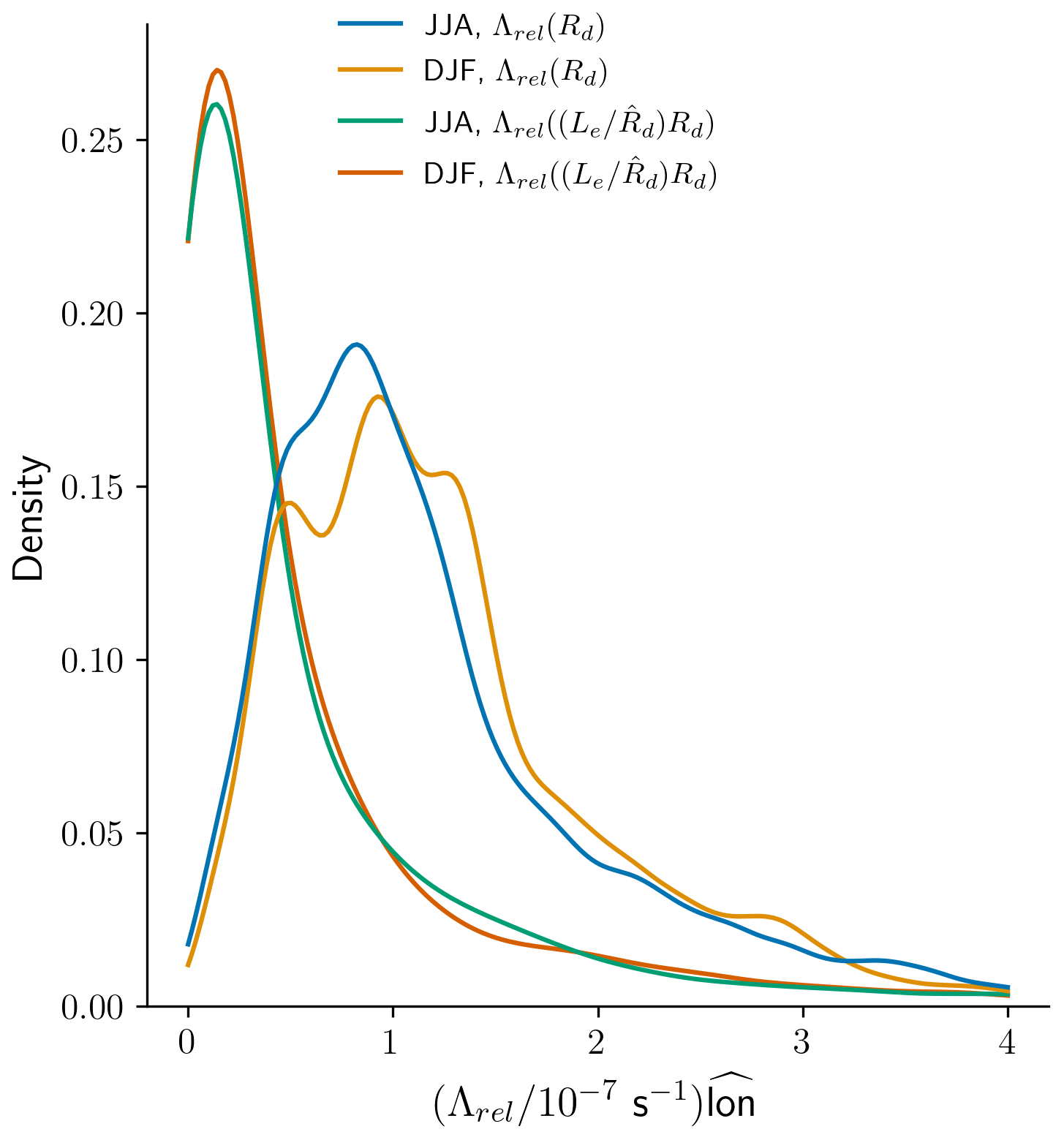
Figure 9 Kernel density estimation of $({\mathrm{\Lambda }}_{\mathrm{rel}}/{\mathrm{10}}^{-\mathrm{7}}$ s${}^{-\mathrm{1}})\widehat{\text{lon}}$, where $\widehat{\text{lon}}$ is a normalised longitude. The four curves represent the dissipation rate Λ_rel depending on the chosen eddy length scale and season (DJF or JJA). Values over the equator band between 5^∘ S and 5^∘ N are not included here.

Figure 8c and d show the dissipation rate that depends on the e-folding length scale, $(L_{\mathrm{e}}/{\widehat{R}}_{\mathrm{d}})R_{\mathrm{d}}$. We see that ${\log }_{\mathrm{10}}({\mathrm{\Lambda }}_{\mathrm{rel}}/{\mathrm{10}}^{-\mathrm{7}}$ s⁻¹) is largely negative, except over the equatorial region. Throughout the Southern Ocean and western boundaries, we find that Λ_rel is around 10 %–25 % the size of 10⁻⁷ s⁻¹. We also see that the pattern is similar to that seen in Λ_rel(R_d) (Fig. 8a, b), particularly across the northwest Atlantic and Southern oceans. This is clearly because the spatial pattern of the chosen eddy length scale (R_d or $(L_{\mathrm{e}}/{\widehat{R}}_{\mathrm{d}})R_{\mathrm{d}}$) are similar, since $(L_{\mathrm{e}}/{\widehat{R}}_{\mathrm{d}})R_{\mathrm{d}}$ depends on R_d.

Contrasting the two choices of eddy length scale is summarised using a density plot of $({\mathrm{\Lambda }}_{\mathrm{rel}}/{\mathrm{10}}^{-\mathrm{7}}$ s${}^{-\mathrm{1}})\widehat{\text{lon}}$ in Fig. 9. Here, we have weighted ${\mathrm{\Lambda }}_{\mathrm{rel}}/{\mathrm{10}}^{-\mathrm{7}}$ s⁻¹ with a normalised longitude ($\widehat{\text{lon}}=\text{lon}/\text{max(lon)}$), where the largest weight is at the lowest latitude. The density of dissipation rates depending on $(L_{\mathrm{e}}/{\widehat{R}}_{\mathrm{d}})R_{\mathrm{d}}$ are skewed to the left and exhibit a narrow range centred around 0.2. The density of the dissipation rate depending on R_d is shifted to the right and displays a wider range of values centred close to 1. What Fig. 9 shows is that the dissipation rate due to relative wind stress may lie somewhere between $\mathrm{2}\times {\mathrm{10}}^{-\mathrm{8}}$ s⁻¹ and $\mathrm{4}\times {\mathrm{10}}^{-\mathrm{7}}$ s⁻¹.

6 Summary and discussion

In this work we have presented a constrained eddy energy dissipation rate for a well-known and important mesoscale dissipation pathway, relative wind stress. Deriving this dissipation rate draws on our fundamental understanding of relative wind stress damping, vertical eddy structure, and eddy energy. The intention with this dissipation rate is for it to fit into an existing eddy energy budget-based eddy parameterisation (e.g. GEOMETRIC) and offer improvements to the relatively unconstrained and spatially homogenous dissipation rate currently employed.

Before the proposition of a dissipation rate, an approximate expression for relative wind stress damping, termed P_rel, was found (see Sect. 2.1). Several assumptions were made to help achieve this expression found in Eq. (11): mesoscale eddies are, on average, Gaussian in shape over the global ocean (Chelton et al., 2011); and the wind field is constant in strength and direction (Duhaut and Straub, 2006). Thereafter, P_rel is used to predict the decay of baroclinic eddy energy in an analytical two-layer model, which is described in Sect. 2.2. The analytical model is chosen to represent a mesoscale eddy with a first baroclinic mode structure, consistent with the first baroclinic mode containing a high portion of eddy energy. Then, comparing the evolution of eddy energy in the analytical model with a general circulation model shows that the expression for relative wind stress damping can approximate the decay of eddy energy well in each eddy type up to 150 d (Fig. 3). However, it is important to highlight that these results are dependent on our choice of model parameters. For example, while the numerical model diverges from the analytical around day 150, making changes to the eddy amplitude could affect the timescale of divergence. To quantify what these changes may lead to would require additional experiments. Nevertheless, we would still expect damping by relative wind stress to be the same across each model due to the matching of eddy amplitude.

The key component of this work lies in the proposed dissipation rate for eddy energy due to relative wind stress, outlined in Sect. 5. The dissipation rate Λ_rel culminates from the theory given in Sect. 2 and the verification of P_rel through the use of a general circulation model in Sect. 4. Deriving the dissipation rate Λ_rel in Eq. (26) is based on a simple two-layer analytical model that exhibits a first baroclinic mode structure. This model is chosen because the eddy sea surface height reflects the movement of the first baroclinic mode and can, as such, represent a large portion of eddy energy (Chelton et al., 1998). An analytical expression for total eddy energy E is then calculated from the two-layer theory. From this, we are able to construct an eddy energy dissipation rate due to relative wind stress, ${\mathrm{\Lambda }}_{\mathrm{rel}}=\left|P_{\mathrm{rel}}\right|/E$. This dissipation rate is assumed to depend on available potential energy in the thermocline, and not kinetic energy. So whilst relative wind stress damps the surface geostrophic motion, the greater dynamic impact is for relative wind stress to relax the eddy thermocline displacement and damp potential energy.

A global map of the dissipation rate is presented in Sect. 5 along with the terms that contribute to it. The eddy length scale is considered to be either the first baroclinic Rossby radius of deformation (R_d), acquired by solving a typical eigenvalue problem, or an e-folding length scale $\left(\right(L_{\mathrm{e}}/{\widehat{R}}_{\mathrm{d}}\left)R_{\mathrm{d}}\right)$, computed using data from Chelton et al. (2011). The two eddy length scales help to form a range of values that Λ_rel could take. The dissipation rate Λ_rel is shown in Fig. 8 normalised by a constant dissipation rate 10⁻⁷ s⁻¹ on a log ₁₀ plot. For R_d, we find that Λ_rel is greater than 10⁻⁷ s⁻¹ across much of the ocean, with hotspots throughout the Southern Ocean, tropics, and equatorial regions. In the western boundary currents, Λ_rel is closer to 10⁻⁷ s⁻¹. For $(L_{\mathrm{e}}/{\widehat{R}}_{\mathrm{d}})R_{\mathrm{d}}$, Λ_rel is less than 10⁻⁷ s⁻¹ over most of the ocean except the equatorial region. However, Λ_rel still comprises up to a quarter of 10⁻⁷ s⁻¹ in regions like the Southern Ocean and western boundaries. Enhanced eddy energy dissipation in the Southern Ocean could impact heat and mass transport (Meijers et al., 2007; Stewart and Thompson, 2015), the exchange of heat and carbon at the air–sea interface (Villas Bôas et al., 2015; Pezzi et al., 2021), and Antarctic sea-ice cover (Munday et al., 2021). Seasonal variations are also present in the dissipation rate, particularly in eddy rich regions, and are consistent with changes in wind speed and stratification. High frequency wind events can also take place (Zhai et al., 2012), which may significantly modulate eddy energy dissipation in some regions. In addition to the interpretation of the dissipation in Fig. 8, validation of these values could be made in a further study through the computation of eddy available potential energy (von Storch et al., 2012) and use of an eddy detection method (Chelton et al., 2011) to quantify wind power input.

The dissipation rate is based on a simple energy budget derived from a two-layer analytical model, which by design neglects many phenomena that take place in the ocean, such as instabilities and wave dynamics. In the time evolution of total eddy energy (Fig. 3), the predicted and MITgcm results were shown to diverge around day 150 in each eddy type. Total eddy energy in MITgcm was found to undergo an exponential-like decay for around 20 d, which corresponded to a change in eddy shape (Fig. 4). A foundation of the prediction method assumes that the baroclinic eddy remains circular; however, this is clearly not the case. The MITgcm eddy begins as a coherent structure and then transitions into two smaller eddies. The splitting of a baroclinic eddy is due to baroclinic instability and leads to the formation of two barotropic eddies via barotropisation (Ikeda, 1981; Dewar et al., 1999). This suggests that our predictive method could benefit from including an additional model that accounts for a smooth transition to the two smaller barotropic eddies. Indeed, the timescale for this transition could depend on a baroclinic mode timescale and might even depend on eddy polarity. Whether accounting for this process in this prediction method is important for long climate timescales is something that could be investigated in future work.

An alternative approach to the one taken in this paper might be to employ a different representation for the first baroclinic mode, and therefore analytical and numerical setups. In this work we followed the ideas of Wunsch (1997), where the first baroclinic mode is computed using a flat bottom and horizontal bottom velocities are not zero. The choice of the two-layer model and numerical setup is justified by the flat bottom first baroclinic mode. However, a further possibility could be surface modes (de La Lama et al., 2016). Surface modes can be computed over variable topography, and horizontal velocities at the bottom tend to be smaller than if a flat bottom is assumed. An analytical model that provides these surface modes could take the form of the two-layer quasi-geostrophic equations (Cushman-Roisin and Beckers, 2006), whilst a numerical setup may simply resemble an exponential decay from the surface to the bottom. Furthermore, surface modes may even provide a value for the Rossby radius of deformation that sits between our computed values of R_d and $(L_{\mathrm{e}}/\widehat{R_{\mathrm{d}}})R_{\mathrm{d}}$ (LaCasce and Groeskamp, 2020). The nature of surface modes thus do seem appealing. Yet, the idealised two-layer model we use in this study certainly comes with a number of benefits, not least its relatively simple analytical theory, which might not be the case in a quasi-geostrophic model.

This study presents a constrained eddy energy dissipation rate due to relative wind stress damping. Although relative wind stress is not the only mechanism associated with eddy energy dissipation, its focus in this study is grounded in the effects it has on ocean dynamics and ocean processes (Seo et al., 2016; Wu et al., 2017; Renault et al., 2019). A further advantage of this work is having a simple analytical expression for this dissipation rate that can be applied to ocean datasets. Being able to then illustrate the global variability in the eddy energy dissipation rate due to relative wind stress enables the discussion of possible implications this could have on wider climate processes. Areas of immediate future work should look to determine a reasonable approximation for eddy length scale and examine the impacts of this dissipation rate in a global ocean model. Furthermore, we hope the work here can provide the basis for similar studies looking to constrain an eddy energy dissipation rate, improving the energetics and flow in global ocean models.