Response of the Arctic sea ice–ocean system to meltwater perturbations based on a one-dimensional model study

A one-dimensional coupled sea ice–ocean model is used to investigate how the Arctic Ocean stratification and sea ice respond to changes in meltwater. In the control experiments, the model is capable of accurately simulating seasonal changes in the upper-ocean stratification structure compared with observations, and the results suggest that ocean stratification is important for ice thickness development during the freezing season. The sensitivity experiments reveal the following: (1) a decrease in meltwater release weakens ocean stratification and creates a deeper, higher-salinity mixed layer. (2) Meltwater reduced ice melting by 17 % by strengthening ocean stratification. (3) The impact of meltwater released during the previous melting season on ice growth in winter depends on the strength of stratification. After removing all the meltwater during the summer, ice formation in areas with strong stratification increased by 12 % during the winter, while it decreased by 43 % in areas with weak stratification. (4) In some areas of the Nansen Basin where stratification is nearly absent, the warm Atlantic Water can reach the ice directly in early spring, leading to early melting of the sea ice in winter if all meltwater is removed from the model. These findings contribute to our understanding of the complex interactions between ocean stratification, meltwater and sea ice growth and have important implications for climate models and future change prediction in the Arctic.

1 Introduction

The upper Arctic Ocean is strongly stratified with primarily ice coverage and a high volume of freshwater input (Rawlins et al., 2010; McClelland et al., 2012; Rudels, 2015). The Arctic Ocean consists of three main layers. The top layer is a cold and fresh surface layer. The intermediate layer is a cold halocline layer (CHL), which is characterized by gradually increasing salinity, and the bottom layer is a relatively warm and salty Atlantic Water (AW) layer. This stratification pattern is crucial for the existence of Arctic sea ice, as the fresh surface layer and CHL protect the ice cover from the heat stored in the AW layer below (Rudels et al., 1996; Steele and Boyd, 1998; Martinson and Steele, 2001; Rudels et al., 2005). Freshwater flux from river runoff, positive net precipitation, relatively fresh Pacific inflow and seasonal ice melt are critical factors that maintain this stratification (Haine et al., 2015; Carmack et al., 2016).

Ocean–ice heat fluxes play a crucial role in modulating the Arctic sea ice growth–melt cycle (Zhong et al., 2022), with half of the total heat flux absorbed by the sea ice originating from the ocean (Carmack et al., 2015). The very strong density stratification at the base of the mixed layer (ML) in the Canada Basin greatly impedes surface layer deepening and thus limits the flux of deep ocean heat to the surface, which could influence sea ice growth and decay (Toole et al., 2010). Linders and Björk (2013) note that ocean stratification is mostly important for ice growth during the growing season because areas with weak stratification have larger ocean–ice heat fluxes, resulting in less ice formation during winter. Davis et al. (2016) use a one-dimensional model to show that the sea ice in the Eurasian Basin is more sensitive to changes in vertical mixing than that in the Canada Basin due to its weaker ocean stratification.

Ice melting is particularly important for seasonal changes in stratification and ocean–ice heat fluxes in the Arctic Ocean (Jackson et al., 2010; Toole et al., 2010; Linders and Björk, 2013; Hordoir et al., 2022), as meltwater makes a significant contribution to the seasonal changes in freshwater balance in the Arctic Ocean. The external freshwater sources of the Arctic Ocean mainly include Pacific inflow, precipitation minus evaporation and river runoff, with a total annual inflow of approximately 9400 ± 490 km³. The annual outflow volume through oceanic gateways, primarily comprising the Fram Strait, Davis Strait, and Fury and Hecla Strait, is approximately 8250 ± 550 km³. Thus, the annual net freshwater flux from the external sources into the Arctic Ocean is about 1200 ± 730 km³ (Haine et al., 2015). The internal sources of liquid freshwater mainly originate from the melting and freezing processes. Approximately 13 400 km³ of freshwater freezes during winter, and 11 300 km³ of freshwater enters the ocean through ice melting (Haine et al., 2015). Consequently, an average of 1.2 m of freshwater is temporarily deposited into the Arctic Ocean surface during each summer by melting (Haine et al., 2015), which separates the surface ML from the near-surface temperature maximum (NSTM). In winter, surface freshwater is recycled via ice formation and weakening ocean stratification (Peralta-Ferriz and Woodgate, 2015); meanwhile, vertical convection caused by brine rejection or storm-driven mixing can erode the NSTM layer, entraining warm water upward and impeding winter ice formation (Steele et al. 2011; Jackson et al. 2012; Timmermans, 2015; Smith et al., 2018).

Meltwater from the sea ice has a comparatively low density and therefore accumulates in the top ocean layer, strengthening the upper-ocean stratification. Due to the stabilizing of the cold halocline, the ocean heat flux available to melt sea ice decreases, which in turn hinders sea ice melting (Zhang, 2007), which is a negative sea ice–ocean feedback (Bintanja et al., 2013). Zhang (2007) suggests that this negative sea ice–ocean feedback can explain the anomalous increase in Antarctic sea ice extent before the 2010s. However, there are almost no quantitative studies on the role of meltwater in the ice–ocean coupled system of the Arctic Ocean, although many previous studies have investigated the effects of increased freshwater flux by adding freshwater flux to the ocean surface in models to represent increased runoff or precipitation (Nummelin et al., 2015, 2016; Davis et al., 2016; Pemberton and Nilsson, 2016).

To enhance the comprehension of the role of the meltwater in the sea ice–ocean system, we use a one-dimensional coupled sea ice–ocean model and modify the source code to control the release of meltwater to the ocean to quantitatively assess the responses of the ocean and sea ice to different amounts of meltwater release to the ocean. One-dimensional models have been widely used in previous studies of the Arctic Ocean's vertical structure and ice cover (Killworth and Smith, 1984; Price et al., 1986; Bitz et al., 1996; Björk, 2002a, b; Peterson et al., 2002; Linders and Björk, 2013; Nummelin et al., 2015, 2016; Davis et al., 2016). A one-dimensional model is simplistic because it does not take advection processes into account; however, it usually provides a reasonable simulation of upper-ocean stratification that matches observations well in a short simulation time (Toole et al., 2010; Linders and Björk, 2013).

Additionally, the intensity of stratification varies across the Arctic Ocean, with a gradual weakening from the Canada Basin towards the Eurasian Basin. In the Canada Basin, a lower-saline upper layer results in a well-developed and persistent cold halocline (Toole et al., 2010). In contrast, the cold halocline layer is quite weak or even absent in some areas of the Eurasian Basin (Rudels et al., 1996; Steele and Boyd, 1998; Björk, 2002b), such as those close to Svalbard in the Nansen Basin, where the warm AW is more easily mixed upward and reaches the ice cover (Rudels et al., 2005). Previous research has suggested that brine-driven surface convection could entrain the AW heat upward in the Eurasian Basin (Polyakov et al., 2013a), while the strong stratification impedes this convection process in the Canada Basin (Toole et al., 2010). Given the considerable spatial variability in the stratification strength across the Arctic Ocean, the impact of meltwater is expected to vary regionally. Thus, this study investigates regional variations in the effect of meltwater on the ocean and sea ice by experimenting with the initial temperature and salinity profiles from multiple stations in the Arctic Ocean.

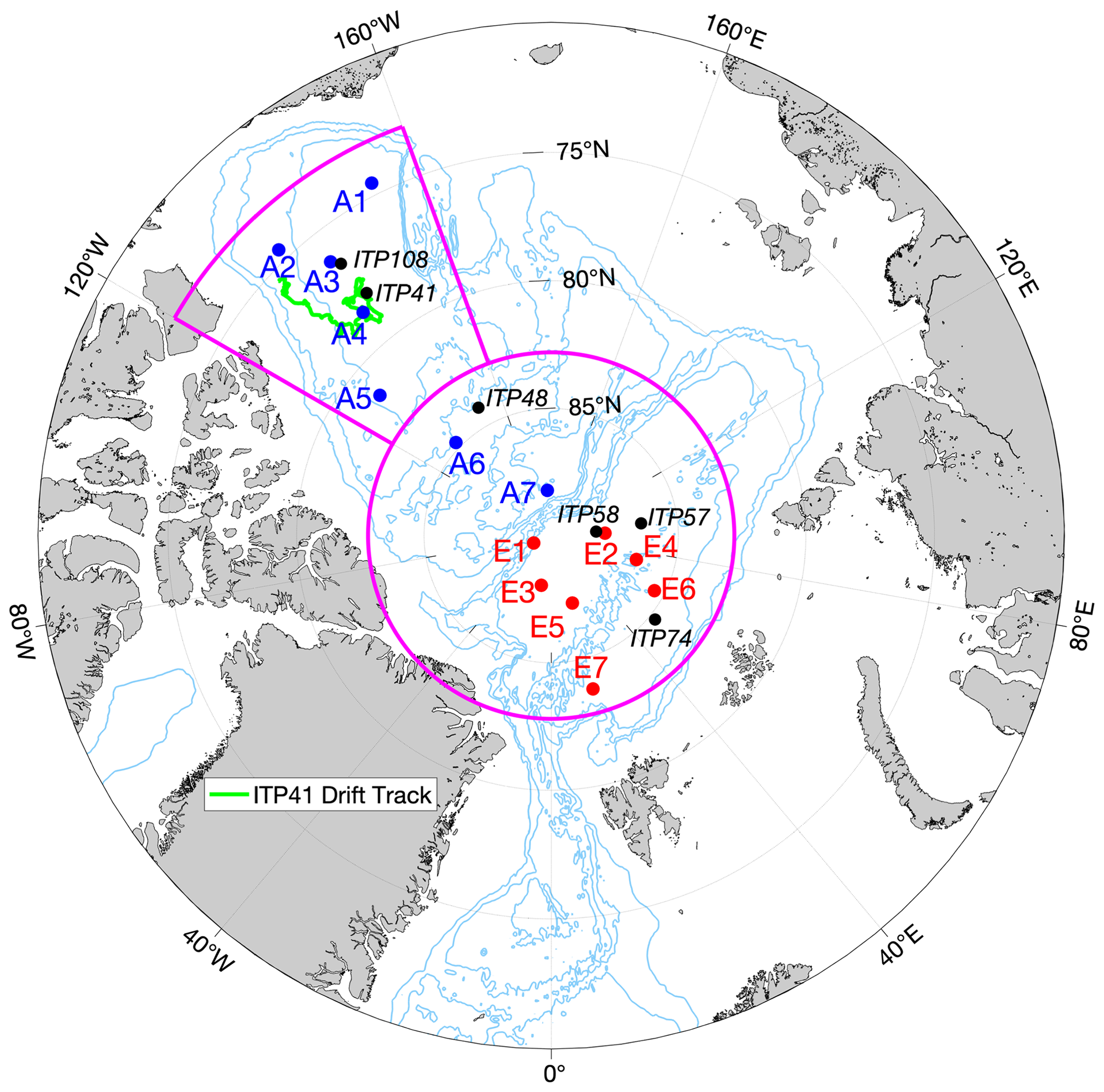
Figure 1 Locations of the ITP data used as initial profiles in the model. Stations A1–A7 are located in the Amerasian Basin (indicated by the blue dots), and E1–E7 are located in the Eurasian Basin (indicated by the red dots). The black dots represent the ITPs used for comparison with the simulations. The green line represents the trajectory of ITP 41. The bathymetry is from ETOPO2. The same atmospheric forcing field, derived from the 2011–2020 average for the specific region outlined by the solid magenta line, is utilized in all experiments.

Table 1 Details of the ice-tethered profile (ITP) records used in the model.

The paper is organized as follows: Sect. 2 details the model setup and the sensitivity experiments. Section 3 presents the model results and discusses how the ocean and sea ice respond to reduced meltwater release. A discussion is provided in Sect. 4. Section 5 reviews the conclusions.

2 Model description and sensitivity experiments

2.1 Coupled sea ice–ocean model

We use a one-dimensional coupled sea ice–ocean model based on the Massachusetts Institute of Technology general circulation model (MITgcm; Marshall et al., 1997) to investigate the influence of meltwater in a coupled ice–ocean system in the Arctic Ocean. The water column in the model extends from the surface down to a depth of 300 m, and the vertical grid has a uniform thickness of 1 m. The bottom boundary condition is zero flux, meaning that there is no exchange between the upper water column and the water below 300 m. The ocean model utilizes the nonlinear equation of state of Jackett and McDougall (1995) and the nonlocal K-profile parameterization (KPP) vertical mixing scheme of Large et al. (1994). Shaw and Stanton (2014) show that the vertical diffusivity in the deep central Canada Basin averages near-molecular levels, ranging between 2.2 × 10⁻⁷ and 3.4 × 10⁻⁷ m² s⁻¹, and Fer (2009) found that vertical diffusivity ranges between 10⁻⁶ and 10⁻⁵ m² s⁻¹ in the Eurasian Basin. The background vertical diffusivity of the model used in this study is set to 10⁻⁶ m² s⁻¹, which is a representative value in the central Arctic Ocean and has been applied to several one-dimensional models used to study the Arctic Ocean (Linders and Björk, 2013; Nummelin et al., 2015; Davis et al., 2016).

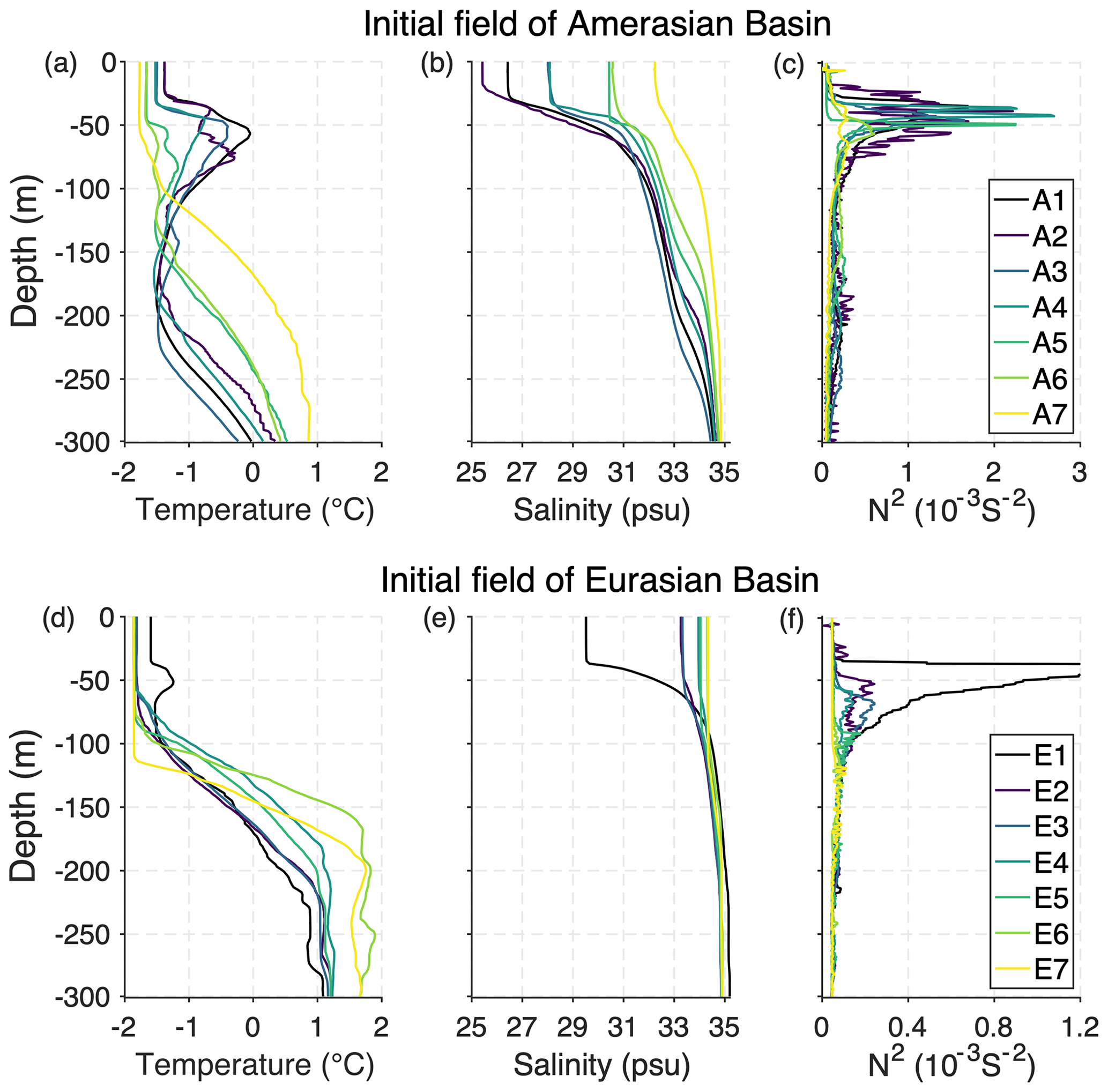
Figure 2 The observed temperature (a, d) and salinity (b, e) profiles obtained from ITPs in the Arctic Ocean, which are used as the initial profiles in the model. The corresponding buoyancy frequency values (c, f) for each station are also displayed. The dates of the observations for each station is shown in Table 1.

Figure 3 Simulated net ocean freshwater flux and time series of the upper 50 m salinity at station A1. (a) Time series of the net freshwater flux at the sea surface (the sum of freshwater fluxes caused by ice melting/freezing and surface freshwater forcing). The negative values represent the freshwater entering the ocean. In the legend, the percent refers to the magnitude of the meltwater input anomaly in the meltwater perturbation (MWP) runs. (b) Time series of the upper 50 m salinity for the control run at station A1. (c–g) Time series of the upper 50 m salinity for MWP runs at station A1. The black lines in (b–g) indicate the MLDs.

The sea ice package is based on a variant of the viscous-plastic sea ice model (Losch et al., 2010) and is combined with the thermodynamic sea ice model of Winton (2000) and Bitz and Lipscomb (1999). Although the one-dimensional model includes a dynamic sea ice model, sea ice changes are only determined by thermodynamic processes. The model considers two equally thick ice layers: the upper layer has a variable specific heat resulting from brine pockets, and the lower layer has a fixed heat capacity. The heat fluxes at the ice top and bottom are

$$\begin{array}{}\text{(1)}& {\displaystyle }{F}_{\mathrm{top}}=F_{\mathrm{s}}\left(\mathit{\alpha }\right)-F_{{\mathrm{s}}_{\mathrm{ice}}},\text{(2)}& {\displaystyle }{F}_{\mathrm{bot}}=F_{{\mathrm{b}}_{\mathrm{ice}}}-F_{\mathrm{b}},\end{array}$$

where F_s is the surface heat flux absorbed by the ice, $F_{{\mathrm{s}}_{\mathrm{ice}}}$ is the conductive heat flux from the upper layer of the sea ice to the ice surface and $F_{{\mathrm{b}}_{\mathrm{ice}}}$ is the conductive heat flux from the ice bottom to the lower layer of the sea ice. F_b is the ocean–ice heat flux:

$$\begin{array}{}\text{(3)}& F_{\mathrm{b}}=c_{\mathrm{sw}}{\mathit{\rho }}_{\mathrm{sw}}\mathit{\gamma }\left(T_{\mathrm{sst}}-T_{\mathrm{f}}\right)u^{*},\end{array}$$

where γ is the heat transfer coefficient, and u^* is the frictional velocity between the ice and water.

The albedo parameterization of this model is dependent on ice thickness (Hansen et al., 1983):

$$\begin{array}{}\text{(4)}& \mathit{\alpha }={\mathit{\alpha }}_{{\mathrm{i}}_{\min }}+\left({\mathit{\alpha }}_{{\mathrm{i}}_{\max }}-{\mathit{\alpha }}_{{\mathrm{i}}_{\min }}\right)\left(\mathrm{1}-e^{-h_{\mathrm{i}}/h_{\mathit{\alpha }}}\right),\end{array}$$

where ${\mathit{\alpha }}_{{\mathrm{i}}_{\min }}=$ 0.1 and ${\mathit{\alpha }}_{{\mathrm{i}}_{\max }}=$ 0.64 are the maximum and minimum ice albedo values, respectively; h_α= 0.65 is the ice thickness for albedo transition; and h_i is the ice thickness.

The net ocean surface heat flux can simply be written as (Steele et al., 2010)

$$\begin{array}{}\text{(5)}& F_{\mathrm{ocean}}=F_{\mathrm{sw}}+F_{\mathrm{b}}+F_{\mathrm{ao}},\end{array}$$

where F_sw is the heat flux from solar radiation, F_b is the ocean-to-ice heat flux and F_ao is the heat flux from the ocean to the atmosphere through the ice-free area (including longwave radiation and sensible and latent heat flux).

2.2 Initial conditions

The model is initialized with a given ice thickness (2.5 m), ice concentration (95 %), and time-averaged temperature and salinity profiles measured by ice-tethered profiles (ITPs) (Krishfield et al., 2008; Toole et al., 2011). The data from 14 ITPs are selected as initial profiles in the model simulations: A1–A7 located in the Amerasian Basin (the blue dots in Fig. 1) and E1–E7 in the Eurasian Basin (the red dots in Fig. 1). Data from the other six ITPs are used to evaluate the simulation (the black dots in Fig. 1), and they are all located close to the simulated stations. The details of the ITP records used in this study are listed in Table 1.

Figure 2 shows the time-averaged vertical profiles of the temperature, salinity and buoyancy frequency from the 14 ITPs. The buoyancy frequencies show that the strength of ocean stratification gradually decreases from the Pacific side towards the Atlantic side (Fig. 2c and f). The vertical temperature profiles at stations A1, A3 and A4 show a temperature maximum at around 50 m in the upper layer, which is the Pacific Summer Water (PSW) that is widely present in the central and western Canada Basin (Shimada et al., 2001; Steele, 2004). The temperature profile at station A2 shows two peaks in the upper layer: one is the NSTM, and the other is the PSW. The initial profile at station A2 was obtained from ITP measurements in the southern Canada Basin in 2007–2008, and due to a strong halocline that year, the NSTM that formed in the summer of 2007 persisted until the spring of 2008 (Jackson et al., 2012). Another noticeable feature is the temperature minimum observed around 175 m in stations A1–A4, which is the Pacific Winter Water (Fig. 2a). Stations A6 and A7 are in the Makarov Basin, and the profiles show a transition feature from Pacific Water to Atlantic Water influence. The upper layer of stations E1–E7 in the Eurasian Basin is characterized by a cold and fresh surface ML overlying a deeper warm ($T>\mathrm{0}{}^{\circ }$) and salty AW layer and weaker ocean stratification than the Amerasian Basin (Fig. 2d–f). Station E1, located at the Lomonosov Ridge, despite being closer to the Eurasian Basin, also has strong stratification features similar to those of the stations in the Amerasian Basin. Stations E6 and E7, in the Nansen Basin, have much weaker salinity stratification than other stations in the Eurasian Basin. These vertical profiles reflect various stratification features across the Arctic Ocean.

2.3 Atmospheric forcing and freshwater input

Atmospheric forcing for the model includes daily 10 m wind speed, 2 m air temperature, 2 m specific humidity, and downward long- and shortwave radiation from the National Centres for Environmental Prediction-Department of Energy (NCEP-DOE) Reanalysis 2, all of which are regionally averaged over the area delineated by the purple boundary in Fig. 1. The averages are calculated over the period of 2011 to 2020 and cover the area defined by the two subareas spanned by 83–90^∘ N latitudes and 0–360^∘ E longitudes (central Arctic Ocean) and 73–83^∘ N latitudes and 200–240^∘ E longitudes (Canada Basin). The same atmospheric forcing is used for all model runs to eliminate the effects of differences in atmospheric forcing. Although the focus of this study is on the meltwater influence in the coupled ocean–sea ice system, freshwater fluxes due to runoff inflow, precipitation minus evaporation, and input or output from straits also contribute to the stratification changes in the Arctic Ocean. Haine et al. (2015) reported that the annual net inflow of freshwater into the Arctic Ocean is approximately 1200 km³ yr⁻¹, and we add this net freshwater inflow to our model on a daily average to represent various freshwater sources other than the meltwater. We compared the differences between experiments with and without external freshwater forcing at stations A1, A6, E2 and E7. In regions with strong stratification, the presence or absence of external freshwater has little impact on the results. However, in weakly stratified regions, like station E7, the differences are more pronounced (refer to the supplementary file for further details).

Figure 4 The time series of temperature (a, c) and salinity (b, d) for the upper 50 m were derived from (a, b) ITP 41 observations and (b, d) simulated values at station A4, respectively. The trajectory of ITP 41 is shown in Fig. 1.

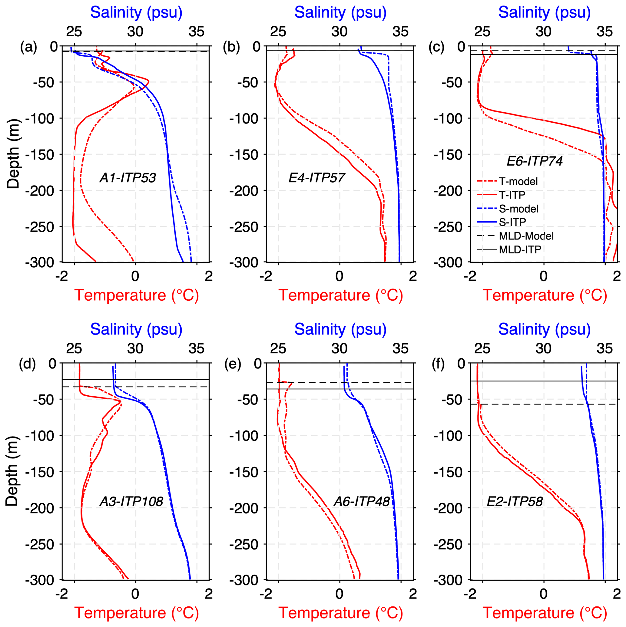
Figure 5 Comparison of the simulated temperature (dotted red line) and salinity (dotted blue line) with the nearby ITP data (solid lines) during summer (a, b, c) and winter (d, e, f). The depth of the ML is indicated by the black lines parallel to the x axis. (a) A4 and ITP 41 in August. (b) E4 and ITP 57 in August. (c) E6 and ITP 74 in August. (d) A3 and ITP 108 in April. (e) A6 and ITP 48 in January. (f) E2 and ITP 58 in April.

2.4 Sensitivity experiments

To investigate the impact of the release of meltwater on ocean stratification and sea ice, a total of six experiments were conducted at each station for a simulation period of 1 year, starting on 1 May and ending on 30 April the next year. The first is the control run, and the other five experiments are the meltwater perturbation (MWP) runs with 0 %, 20 %, 40 %, 60 % and 80 % meltwater release into the ocean. The experiments started on 1 May with the objective of conducting a full melting period followed by a complete freezing phase in the model, which helps to better investigate the effects of meltwater on sea ice melting in summer, as well as its impact on subsequent freezing in winter. In the coupled ice–ocean model, the meltwater flux of a time step (600 s) is determined by the freshwater content of the sea ice before and after a time step. In its initial state, the freshwater content of the sea ice is as follows:

$$\begin{array}{}\text{(6)}& W_{\mathrm{frw}}={\mathit{\rho }}_{\mathrm{Ice}}\cdot H_{\mathrm{Ice}},\end{array}$$

where W_frw is the mass of freshwater initially present in the ice, ρ_Ice is the density of the ice (ρ_Ice= 900 kg m⁻³) and H_Ice is the initial ice thickness. The meltwater entering the ocean is calculated as follows:

$$\begin{array}{}\text{(7)}& F_{\mathrm{reflx}}=(W_{\mathrm{frw}}-{\mathit{\rho }}_{\mathrm{Ice}}\cdot h_{\mathrm{Ice}})/\mathrm{\Delta }t,\end{array}$$

where F_reflx (kg m⁻² s) is the ocean freshwater flux, and h_Ice is the ice thickness.

In the sensitivity experiments, we scale the freshwater flux by multiplying it by a factor k to control the amount of meltwater release:

$$\begin{array}{}\text{(8)}& F_{\mathrm{reflx}}=k\cdot {\mathit{\rho }}_{\mathrm{Ice}}\cdot (H_{\mathrm{Ice}}-h_{\mathrm{Ice}})/\mathrm{\Delta }t.\end{array}$$

We set k to 0 (MWP 0 % run), 0.2 (MWP 20 % run), 0.4 (MWP 40 % run), 0.6 (MWP 60 % run) and 0.8 (MWP 80 % run).

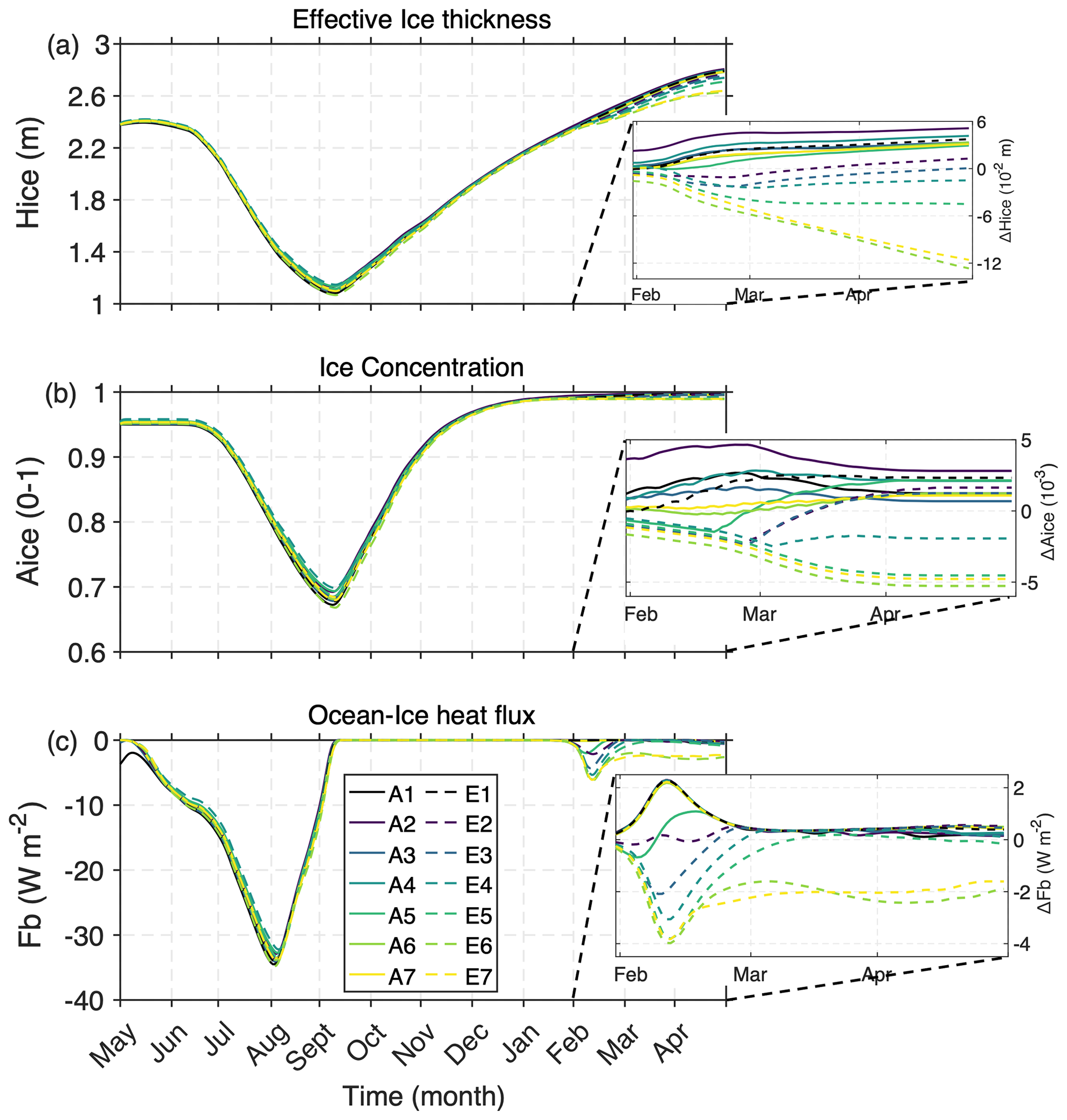
Figure 6 Time series of the (a) effective sea ice thickness (H_ice), (b) ice concentration (A_ice) and (c) ocean–ice heat flux (F_b; negative values represent the heat transfer from the ocean to the ice) for all control runs. The amplified subplot shows the anomalies (each control run minus the average of all control runs) during the months of February to April.

Figure 3a shows the time series of the net ocean freshwater flux, the sum of freshwater fluxes caused by ice melting/freezing and surface freshwater forcing for the six experiments at station A1, in which the negative value represents freshwater entering the ocean. In this model, the surface freshwater flux caused by ice melting/freezing is on average several tens of times larger than the external freshwater forcing. Therefore, Fig. 3a can be regarded as the ocean freshwater flux caused by ice melting/freezing. It is obvious that freshwater flux is negative (positive) during the ice-melting (ice growth) season in the control runs. In the MWP runs, the meltwater flux is artificially reduced during the ice-melting season. As expected, the salinity gradient becomes weaker, and the ML deepens when the release of the meltwater is reduced (Fig. 3b–g). In this study, the mixed layer depths (MLDs) are calculated as the depth at which the potential density relative to 0 dbar initially surpasses the shallowest sampled density by the threshold criterion of Δσ= 0.03 kg m⁻³, according to previous studies (Toole et al., 2010; Jackson et al., 2012; Peralta-Ferriz and Woodgate, 2015).

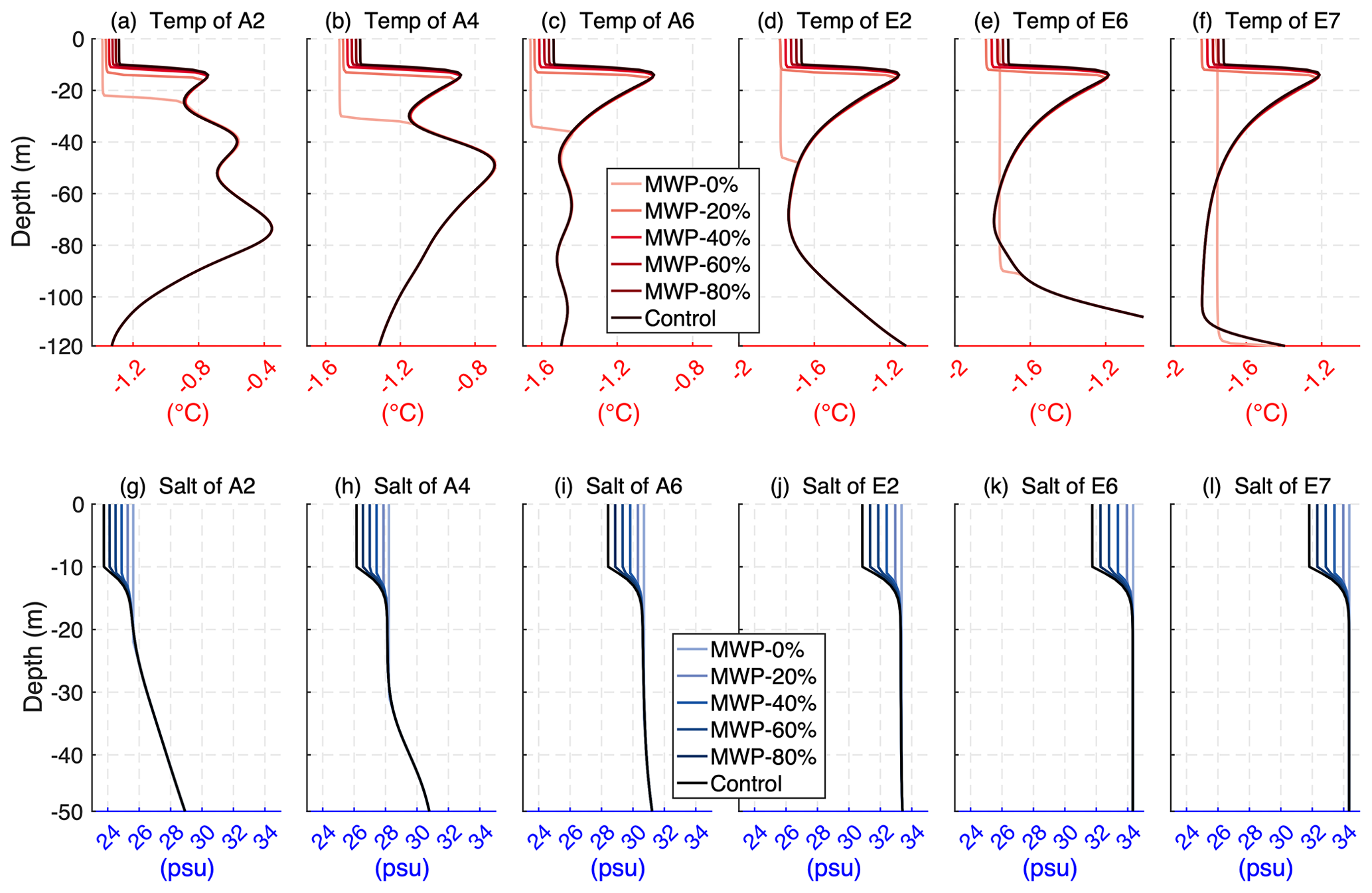
Figure 7 Simulated temperature (a–f) and salinity (g–l) profiles of control runs and MWP runs in mid-August for stations A2, A4, A6, E2, E6 and E7.

3 Results

3.1 Control runs

3.1.1 Upper-ocean thermohaline structure

Figures 4 and 5 show the comparison between the simulated temperature and salinity profiles of the control runs and the ITP observations (the details of the six ITP datasets for comparison with the simulated results are listed in Table 1). The results of the one-dimensional model reproduce the seasonal variations in the vertical temperature and salinity structure in the Arctic Ocean reasonably well. It should be noted that this study does not aim to replicate the variability of the ITP profiles perfectly, as the variability of the Arctic Ocean temperature and salinity structure is influenced not only by surface freshwater fluxes but also by an array of external local forcings, such as high-frequency variations in wind fields, local precipitation or evaporation, horizontal transport of freshwater, and observational errors. Despite some discrepancies between the simulated and observed vertical profiles, the simulations of these ideal experiments are still qualitatively consistent with the observations. Therefore, the simulation results obtained in this study are reliable.

ITP 41 measured relatively complete temperature and salinity data along its pathway (green line in Fig. 1) in the Canada Basin from May 2011 to April 2012, and the data measured by ITP 41 in May 2011 also serve as the initial field for station A4 in the model. Therefore, we compared the complete time series of the temperature and salinity of the ITP 41 observations with the simulations. Both the observations and the simulations show that large quantities of freshwater, primarily meltwater, cover the ocean surface during the melting season, typically lasting from June to September. As a result, a significant salinity gradient forms between the surface water and underlying water layers, creating a new, fresher surface layer (Fig. 4b and d). And the model also successfully reproduces the NSTM at the base of the summer ML, present at approximately 10–20 m (Fig. 4a and c). During the freezing season (October to the next April), brine rejection enhances the turbulence-scale perturbations, leading to a deeper ML, and the NSTM generated during the summer progressively cools and vanishes (Fig. 4a and c).

Furthermore, we compared the simulated values with actual summer and winter observations gathered from select stations in the vicinity of the simulation. Figure 5 shows that the simulated vertical temperature and salinity profiles and MLDs for both summer and winter are similar to the nearby ITP observations. However, the simulated summer NSTM in the Canada Basin is generally cooler than the observations' summer NSTM (Fig. 5a). This discrepancy may lead to an overestimation of winter ice formation in the simulations. In all control runs, the simulated maximum winter MLDs are ∼ 33 m in the Canada Basin, ∼ 43 m in the Makarov Basin, ∼ 67 m in the Amundsen Basin and more than 100 m in the Nansen Basin. These results are comparable to the observations. The observed maximum winter MLDs in the Canada and Makarov basins are 29 ± 12 and 52 ± 14 m, respectively, and those in the Eurasian Basin range from ∼ 50 to over 100 m (Shimada et al., 2001; Peralta-Ferriz and Woodgate, 2015). Both the modeling and the observations show that the MLDs are usually deeper in the Eurasian Basin than in the Canada Basin.

3.1.2 Sea ice and ocean–ice heat flux

Figure 6 shows the temporal development of ice thickness, ice concentration and ocean–ice heat flux in the control runs. The amount of ice melt during the melting season is basically independent of the initial ocean stratification. However, the sea ice growth from February to April shows dependence on the initial ocean stratification (subplot in Fig. 6a). Under the same atmospheric forcing, stations in the American Basin (A1–A7) with well-developed and persistent haloclines have more ice growth (∼ 1.68 m), while stations E6 and E7 in the Nansen Basin have less ice growth (∼ 1.55 m) because the cold halocline is not fully developed there, and, consequently, the higher ocean–ice heat flux from February to April inhibits ice formation (Fig. 6c). Figure 6a shows that in all control runs ice grows beyond the initial conditions, as the model ran for only 1 year and did not reach an equilibrium state. Nevertheless, it is still reasonable for this study because this paper focuses on the anomalies from the control run by perturbing the meltwater.

In the control run, the calculated ocean–ice heat flux in the Canada Basin (stations A1–A7) has an average value of 0.06 W m⁻² during the freezing season and 15.8 W m⁻² during the melting season (Fig. 6c). The observed ocean–ice heat flux from the entire surface heat budget of the Arctic Ocean drift has an average value of 2.2 W m⁻² during winter and 16.3 W m⁻² during summer (Shaw et al., 2009). This comparison indicates that the simulated ocean–ice heat flux is close to the observations in summer but much smaller than the observations in winter. The main reason for this is the omission of horizontal advection in the one-dimensional model. Horizontal heat transport is an important factor in the increase in ocean–ice heat flux in winter, and omitting it from the model will lead to a lower winter ocean–ice heat flux. In summer, the main heat source is the absorption of solar radiation (Perovich et al., 2011), and the surface water temperature is less affected by horizontal heat advection.

As observed by Jackson et al. (2010) and Steele et al. (2011), our model also shows that the NSTM normally deepens, cools and disappears throughout the autumn and winter (Fig. 4). However, it has sometimes been observed as a year-round feature. Jackson et al. (2012) found that when ITP 18 drifted into shallow waters from early to mid-December, the ocean–ice heat flux reached up to 55 W m⁻² (Jackson et al., 2012), reducing sea ice thickness at the end of the 2008 growth season by about 25 % (Timmermans, 2015). Smith et al. (2018) also discovered occasional high values of the winter ocean–ice heat flux (about 100 W m⁻²) in the Canada Basin using ITP and conductivity–temperature–depth (CTD) data from 2015. These high winter sea ice heat fluxes are usually associated with strong wind events (Smith et al., 2018). In this study, all experiments utilized regionally averaged wind fields to eliminate the impact of wind field variability. This may be the reason why our one-dimensional model did not reproduce the episodic high values of the ocean–ice heat flux in winter successfully.

Simulated ocean–ice heat fluxes in the Amundsen Basin (stations E1–E5) and Nansen Basin (stations E6 and E7) have an average value of 0.29 and 1.2 W m⁻² during the freezing season and 15.6 and 16.1 W m⁻² during the melting season (Fig. 6c), respectively. The ocean–ice heat flux in the Eurasian Basin in winter is larger than that in the American Basin, which results in less ice formation in the Eurasian Basin. The results suggest that ocean stratification is a very important factor for ice growth, which agrees with the conclusions of Linders and Björk (2013).

3.2 Meltwater perturbation experiments

3.2.1 Upper-ocean responses

Summertime

Figure 7 shows the temperature and salinity profiles in summer for the MWP and control runs. It is obvious that no release of meltwater has the most pronounced effects, compared with the control run, while the release of a portion of meltwater has a moderate-to-little effect on the upper-ocean structure. The experimental results for some stations in this study are very similar, so this paper discusses the simulation results for six representative stations to show the general behavior of the model and the impact of ocean stratification. Three of the stations are located in the Amerasian Basin (A2, A4 and A6) and three in the Eurasian Basin (E2, E6 and E7).

In the MWP 0 % runs, as no meltwater is released, the upper water is well mixed, the NSTM vanishes, and the temperature and salinity are uniform in the upper layer (down to a depth of several tens of meters) in the Canada Basin to more than 100 m in the Nansen Basin (Fig. 7). As a result of mixing, compared with the control run, salinity increases, and temperature decreases in the ML at stations A1–A7 (such as Fig. 7a–c) and E1–E5 (such as Fig. 7d). However, at stations E6 and E7, the temperature decreases in the upper ML but increases in the lower ML (Fig. 7e, f). The strength of ocean stratification at stations E6 and E7 is very weak, and the removal of all the meltwater leads to the downward transfer of heat stored in the NSTM, which warms the lower ML.

In contrast to the MWP 0 % run, the summer MLDs in the MWP 20 %–80 % runs are no more than 10 m, which implies that a certain amount of meltwater is sufficient to maintain upper-ocean stratification during summer. When all the meltwater is removed from the model, the MLDs can reach 22–44 m in the Americana Basin, 33–90 m in the Amundsen Basin and over 100 m in the weaker stratified Nansen Basin at the end of the melting season (Fig. 8).

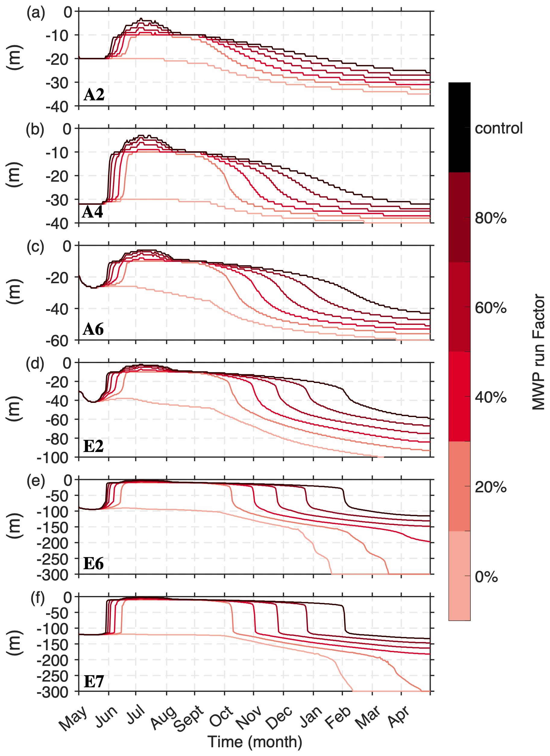
Figure 8 Time series of the MLDs of the control and MWP runs for stations (a) A2, (b) A4, (c) A6, (d) E2, (e) E6 and (f) E7. The color of each line represents the MWP run factor.

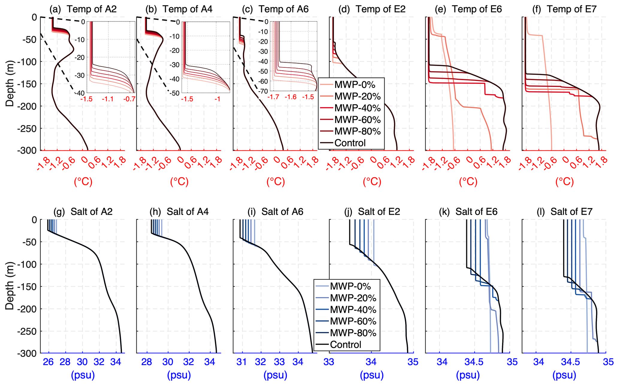
Figure 9 The same as Fig. 7 but in mid-April. The amplified subplots in (a), (b) and (c) display the details of the upper-layer temperature.

Wintertime

Figure 9 shows the temperature and salinity profiles in winter for the MWP and control runs. The extent to which meltwater affects the ocean profile varies with each station (Fig. 9). At each station, the MLD increases following the reduction in the release of meltwater in the previous melting season. Close to the end of the freezing season (mid-April), the MLDs reach their maximum at all stations. At stations A1–A4 in the Canada Basin, the MLDs are 35–44 m for the MWP 0 % run and are still unable to penetrate the PSW layer (Figs. 8a, b and 9a, b). The MLDs in the Amundsen Basin are much larger than those in the Canada Basin in the MWP 0 % runs, approximately 42–170 m (33–99 m in the control run) (Fig. 8d). Nevertheless, they are still unable to reach the core of the warm AW (Fig. 9d).

Stations E6 and E7 in the Nansen Basin show a relatively extreme situation in the 20 % and 0 % runs during winter. The removal of more than 20 % of the meltwater leads to the ML dropping to a depth of more than 300 m (116 and 133 m in the control run, respectively), which can reach the core depth of the warm AW (Fig. 8e and f). This leads to a dramatic change in the structure of the vertical profile when the AW layer is well mixed with the cold water in the upper layers (Fig. 9e, f, k and l). The heat carried by the warm AW will melt the surface ice and release significant amounts of heat into the atmosphere, as described in the next section. The results suggest that the positive buoyancy flux of the meltwater is a significant impediment to the deepening of the ML throughout the simulation.

The above results of the MWP runs imply that the subsurface PSW in the Canada Basin is unable to reach the ice due to strong stratification, even when all the meltwater is removed. However, at some places in the Nansen Basin, such as at stations E6 and E7, which lack a fully developed halocline, meltwater plays an important role in preventing the ML from reaching the AW layer.

3.2.2 Sea ice responses

Melting season

The reduced meltwater release leads to decreases in the summertime effective ice thickness and ice concentration (Fig. 10). In comparison with the control run, the amount of melting ice increases by 21.6 cm (∼ 17 %), 6.4 cm (∼ 5 %), 3.8 cm (∼ 3 %), 2.4 cm (∼ 2 %) and 1.2 cm (∼ 1 %) (averages of all stations) for the MWP 0 %, 20 %, 40 %, 60 % and 80 % runs, respectively, over the entire melting season (Fig. 11a). This suggests that the removal of meltwater promotes ice melting. This implies that the presence of meltwater inhibits sea ice melting during the melting season.

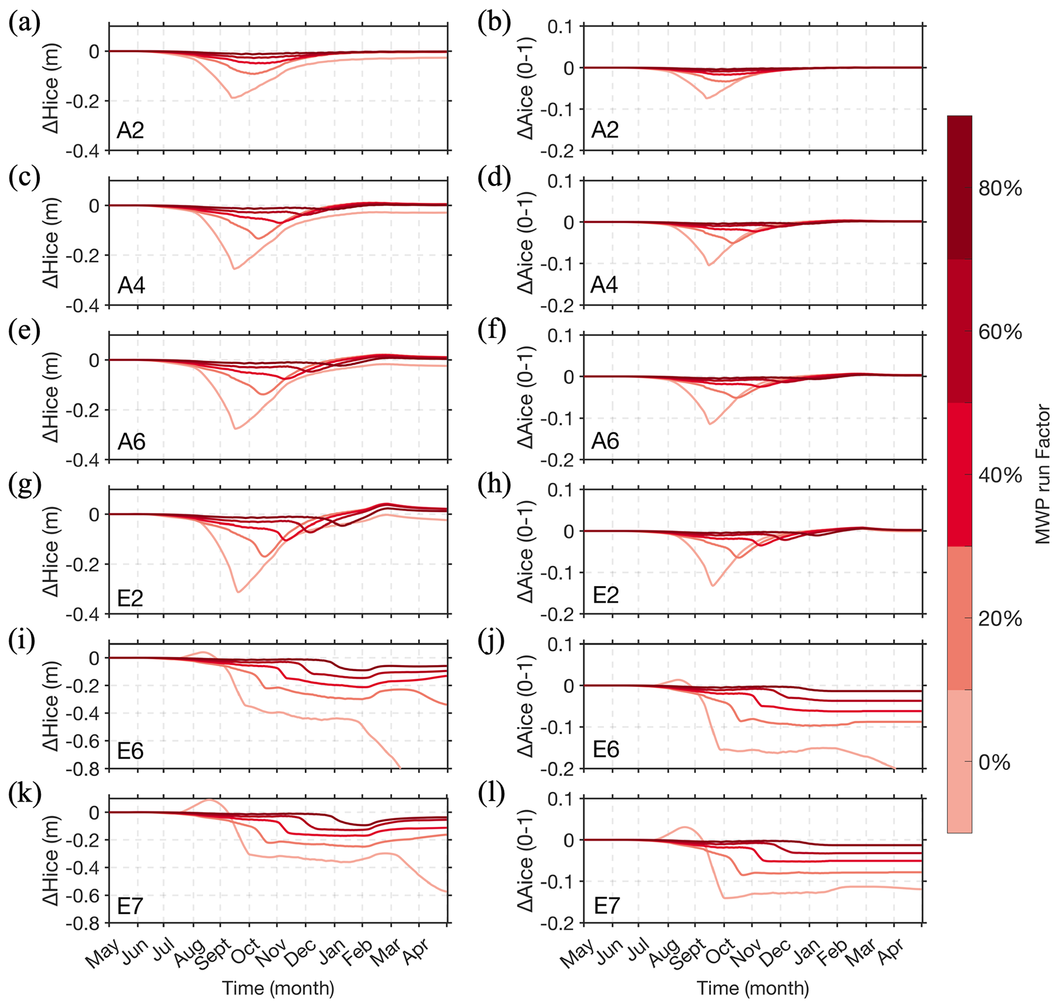
Figure 10 Time series of (a, c, e, g, i, k) the anomalies of effective ice thickness and (b, d, f, h, j, l) anomalies of ice concentration for stations A2, A4, A6, E2, E6 and E7. The anomalies are obtained from the MWP run minus the control run.

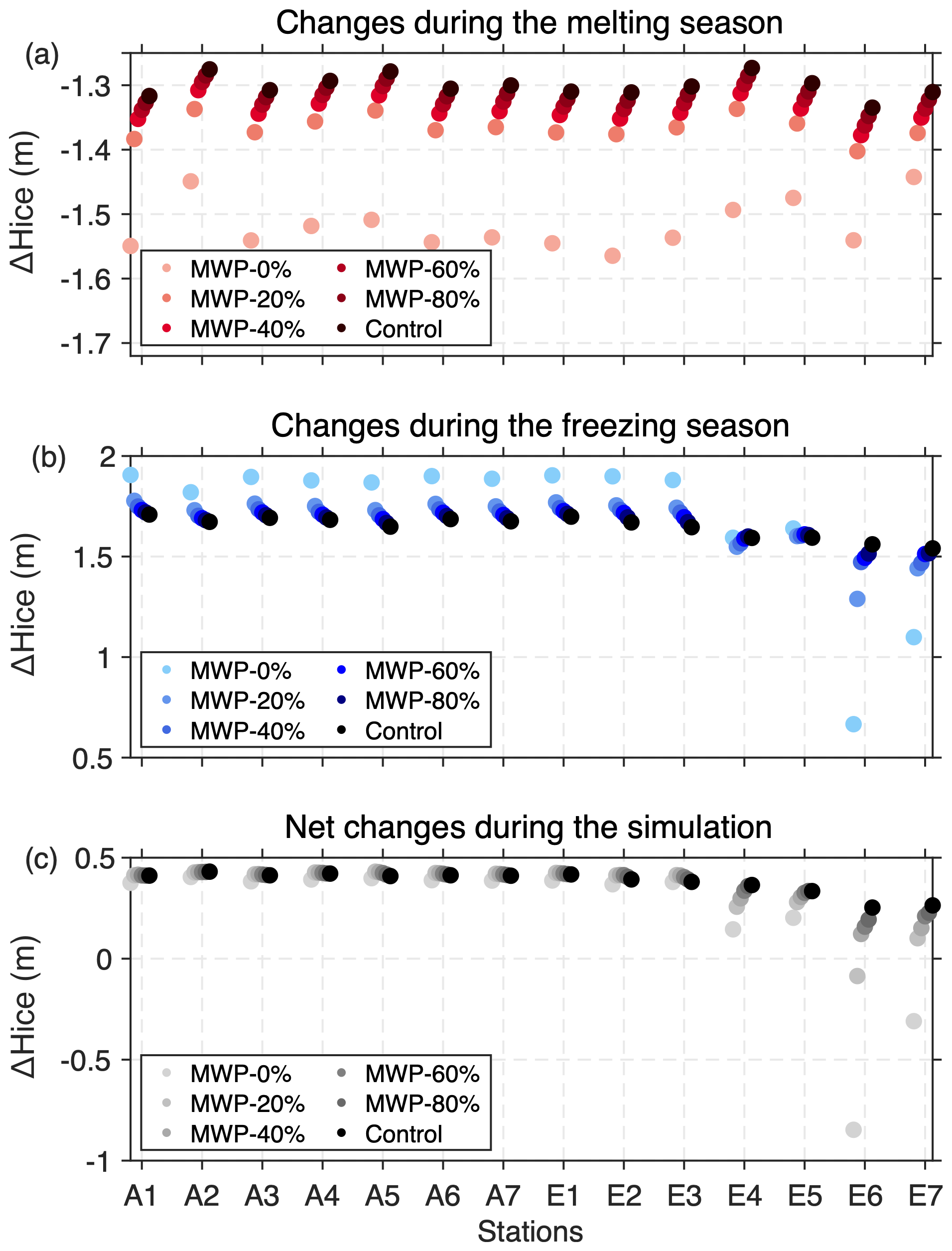
Figure 11 Ice thickness change during the model simulation for all stations. (a) Effective ice thickness change during the melting season. The melting season for each experiment is defined as the period from maximum thickness in May to minimum thickness in September. (b) Effective ice thickness change during the freezing season. The freezing season for each experiment is defined as the period from minimum thickness in September until the end of the simulation.

The time series of the ice top and bottom change rate anomaly between the MWP and the control runs are shown in Fig. 12. The meltwater primarily affects the bottom of the sea ice rather than the top. The meltwater affects bottom melting mainly by impeding vertical mixing of the heat stored in the subsurface. In the MWP 20 % to 80 % runs, as the meltwater release decreases, the summer halocline weakens, allowing more heat in the NSTM to mix upward, resulting in a larger ocean–ice heat flux (Fig. 13, left column).

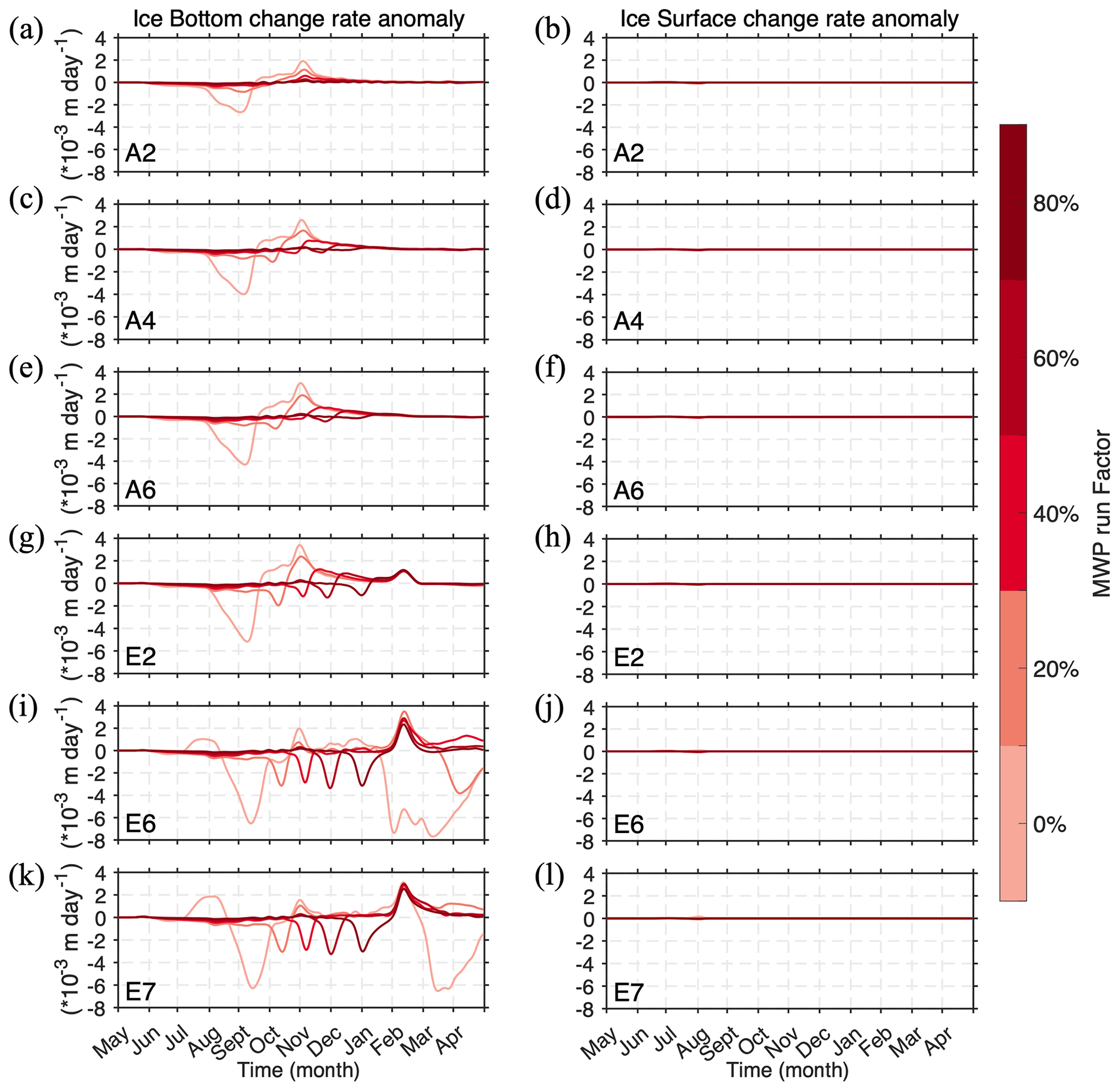
Figure 12 Time series of (a, c, e, g, i, k) the anomalies of the ice bottom change rate and (b, d, f, h, j, l) the anomalies of the ice surface change rate for stations A2, A4, A6, E2, E6 and E7. The anomalies are obtained from the MWP run minus the control run. The negative (positive) values indicate faster (slower) rates of ice decrease in the MWP run compared with the control run. The color of each line represents the MWP run factor.

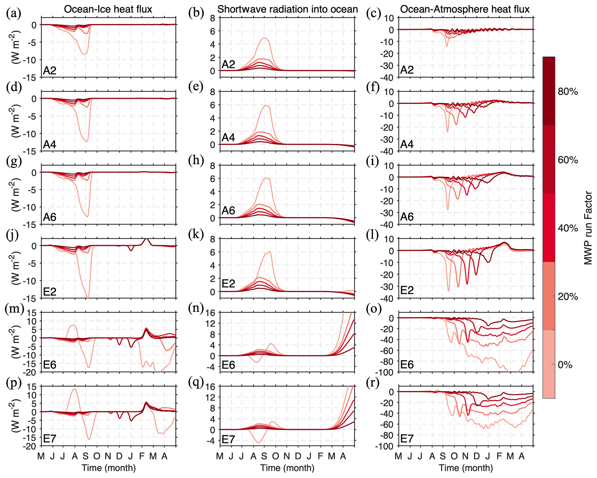
Figure 13 Time series of (left) the anomalies of the ocean–ice heat flux; (middle) the anomalies of shortwave radiation; and (right) the anomalies of the ocean–atmosphere heat flux for stations A2, A4, A6, E2, E6 and E7. The anomalies are obtained from the MWP run minus the control run. The negative (positive) value indicates heat gain (loss) by the ocean in the MWP run compared with the control run. The color of each line represents the MWP run factor.

In the MWP 0 % run, the NSTM promotes ice bottom melting in two ways. The first way, which is dominant in well-stratified areas, is by directly heating the ice bottom by upward mixing in summer, resulting in faster melting. The other way, which is dominant in areas with weaker stratification, is by prolonging the melting season. For example, at station A1, where the stratification is strong, the ice bottom melting rate (Fig. 12a) and ocean–ice heat flux (Fig. 13a) are greater in the MWP 0 % run than in the control run throughout the whole summer, while at stations E6 and E7, where stratification is weak, the ice bottom melting rate (Fig. 12k) and ocean–ice heat flux (Fig. 13p) are not greater in the MWP 0 % run than in the control run until late summer. The reason is that in the strongly stratified stations, even when all meltwater is removed, the stratification is still strong, and the heat stored in the NSTM is mixed only upward and used for ice melting. However, at a weakly stratified station, the heat stored in the NSTM is mixed not only upward but also downward. As shown in Fig. 7a–d, the temperature below 10 m in the MWP 0 % run is lower than that in the control run, indicating limited heat transfer to the underlying layers at strongly stratified stations. Conversely, Fig. 7f illustrates a well-mixed pattern of water temperature between 0–120 m in the MWP 0 % run in station E7. Moreover, the temperature between 60–120 m exceeds that of the control run, suggesting a downward mixing of heat that warms the underlying water layers. The heat transferred downward to the lower ML mixes upward at the onset of the freezing season, which delays the freeze-up and prolongs the melting season.

Freezing season

Figure 11b shows the effective sea ice thickness changes from the minimum value in summer to the end of the freezing season in the sensitivity experiments for all stations. The winter sea ice formation at the strongly stratified stations, A1–A7 and E1–E3, is inversely proportional to the amount of meltwater released in the previous melting season. In the MWP 0 % run, an average increase in sea ice thickness of 21 cm (approximately 12 %) was simulated at these stations compared with the control run. Sea ice formation at stations E4 and E5 is less sensitive to meltwater release changes than that at other stations. In contrast, at the weakly stratified stations, E6 and E7, sea ice formation in the MWP 0 % run decreases by an average of 67 cm (43 %) compared with the control run (Fig. 11b).

At some stations with strong haloclines, e.g., stations A1–A7 and E1–E3, even with all the meltwater removed, the halocline is still strong, which can effectively prevent the ML from deepening in autumn and winter. In particular, the reduction in summer meltwater leads to a weakening or even absent NSTM and insufficient heat stored in the subsurface layer to replenish the heat loss at the surface when autumn arrives, leading to a more rapid cooling of water temperature to the freezing point in autumn and hence increasing ice formation in autumn. This result suggests that the presence of the NSTM effectively hinders sea ice growth in autumn, which is consistent with Toole et al.'s (2010) results. However, at some stations with a weak halocline, e.g., stations E6 and E7, the warm Atlantic Water can reach the surface, which effectively prevents the formation of sea ice. In addition, in March, the ML can reach the depth of the warm AW, and a large amount of heat from the warm AW mixes upward and heats the sea ice, leading to early melting of the sea ice (such as Fig. 10i, k), which allows large areas of open water to exist during the winter (such as Fig. 10j, l). This enables the sea surface to absorb more solar radiation in April (Fig. 13n and q), allowing heat from the warm AW to enter the atmosphere, and the ocean–atmosphere heat flux can reach 70–100 W m⁻² in March at stations E6 and E7 (Fig. 13o and r).

The results indicate that the impact of meltwater released during the previous melting season on winter sea ice growth depends on the strength of stratification, with gradual transitions from promoting to impeding ice growth as the halocline weakens.

Annual net sea ice changes

The annual net changes in the effective ice thickness for the control run and MWP runs at all stations are shown in Fig. 11c. In strongly stratified regions (such as stations A1–A7 and E1–E3), the annual net sea ice change is insensitive to meltwater release (Fig. 11c) because the reduction in meltwater not only leads to more sea ice melting in summer but also leads to an increase in ice formation during winter (Fig. 11b), which offsets the extra ice melting in summer. In weakly stratified regions (stations E4–E7), the annual net sea ice change is more sensitive to meltwater release (Fig. 11c) because the reduction in meltwater induces a deeper ML and enhances the ocean–ice heat flux, resulting in insufficient sea ice formation in winter, which cannot compensate for the extra summer ice melting.

In summary, the above results indicate that meltwater always has an inhibitory effect on ice melting during the melting season. The impact of meltwater released during the previous melting season on the subsequent winter ice formation depends on the strength of stratification. It hinders (promotes) ice formation in areas with strong (weak) stratification. The presence of the meltwater hinders the transfer of heat from the subsurface to the ice cover, which is the main reason for the inhibitory effect of meltwater on sea ice melting during the summer. In addition, the meltwater significantly inhibits ice melt at stations E6 and E7 by hindering the upward heat flux from warm AW in spring.

3.3 Sensitivity experiments with thinner sea ice

In recent decades, it has been observed that Arctic summer sea ice appears to be decreasing rapidly (Perovich et al., 2020), with larger ice-free areas in summer and thinner winter sea ice (Haine and Martin, 2017). Thus, several experiments are conducted using thinner initial ice (1.5 m). To highlight the effects of strong or weak CHLs, we selected stations A3, A6, E2 and E7 to do the thinner ice experiments.

In the control run, the initial thinner ice of 1.5 m completely melts in late July (Fig. 14a), and the maximum ocean–ice heat flux can reach 330 W m⁻² (Fig. 14b). During winter, station E7 produces less sea ice because it possesses a weaker stratification (see Fig. 14a), which is consistent with experiments that had an initial ice thickness of 2.5 m.

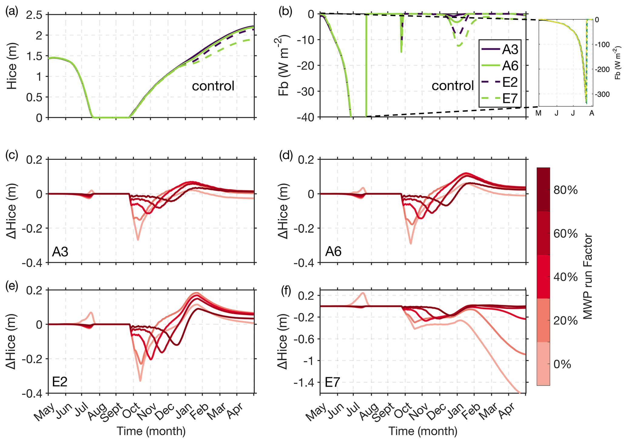
Figure 14 Time series of the (a) effective sea ice thickness and (b) ocean–ice heat flux (negative values represent the heat transfer from the ocean to the ice) for control runs with thinner initial ice thickness. The subplot in (b) shows the time series of ocean–ice heat fluxes between May and August, indicating that ocean–ice heat fluxes can reach a maximum of 330 W m⁻². (c–f) Time series of the anomalies of effective ice thickness for stations A3, A6, E2 and E7. The anomalies are obtained from the MWP run minus the control run.

Compared with the control runs and the MWP 20 %–80 % runs, the sea ice melts more slowly in the MWP 0 % runs (Fig. 14c–f), which contrasts with the experiments with a thicker initial ice. This may be due to the fact that the thinner initial ice contributes to the presence of a larger open ocean during the summer, and increased wind input enhances the mixing level, resulting in more heat being mixed into the deeper ocean. As a result, the heat available for melting sea ice is reduced. Figure 15a–d clearly demonstrate the process: by late July, the temperature of the upper ocean is remarkably lower in the MWP 0 % runs, while the temperature below 10 m is considerably higher compared with the other runs.

During winter, the role of meltwater in hindering the upward mixing of AW is more evident in the thinner initial ice experiments. Removing 40 % of meltwater during the summer in the thinner initial ice runs can enable the upward mixing of the AW (Fig. 16d and h) and subsequent melting of sea ice in winter (Figs. 14f and 17b). However, it would require the thicker initial ice runs to remove over 80 % of meltwater to achieve similar results (Fig. 9f and l).

The thinner ice experiments indicate that as multi-year ice in the Arctic Ocean is replaced gradually by seasonal sea ice, meltwater will play a more significant role in impeding vertical mixing and winter ice melting in the future.

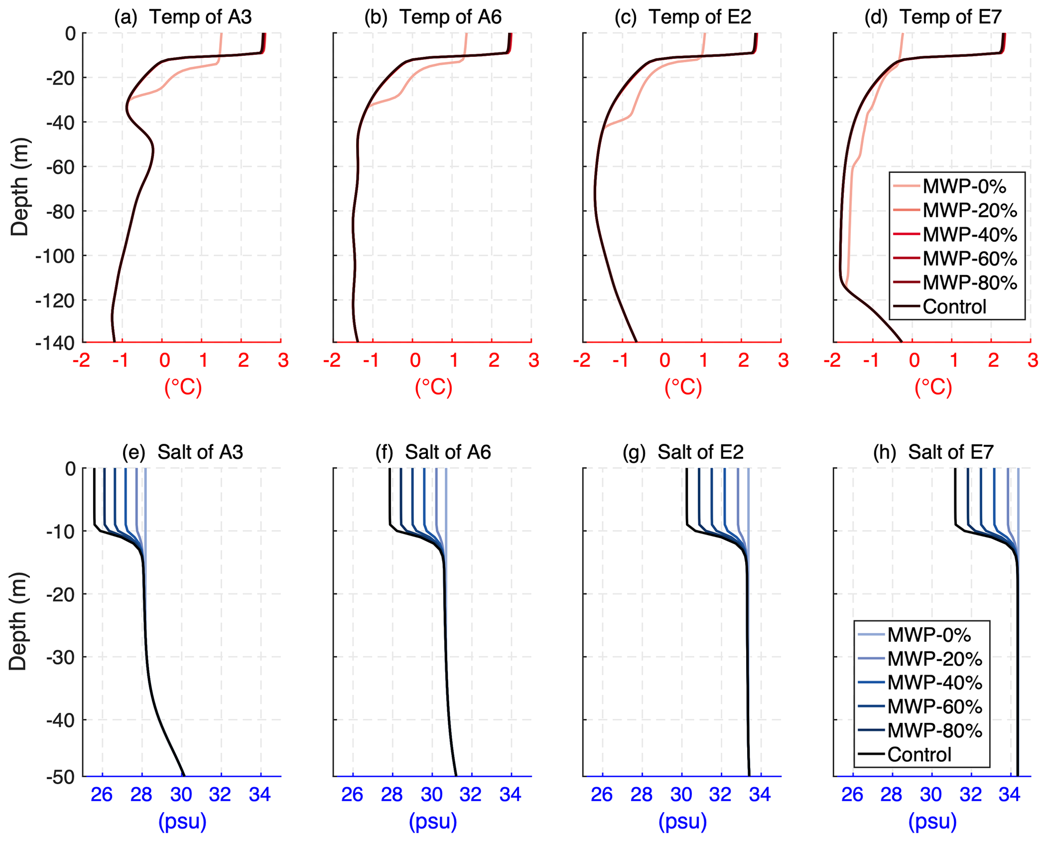
Figure 15 Simulated temperature (a, b, c, d) and salinity (e, f, g, h) profiles of control runs and MWP runs in late July for stations A3, A6, E2 and E7 of the thinner initial ice experiments.

Figure 16 The same as Fig. 15 but in mid-April.

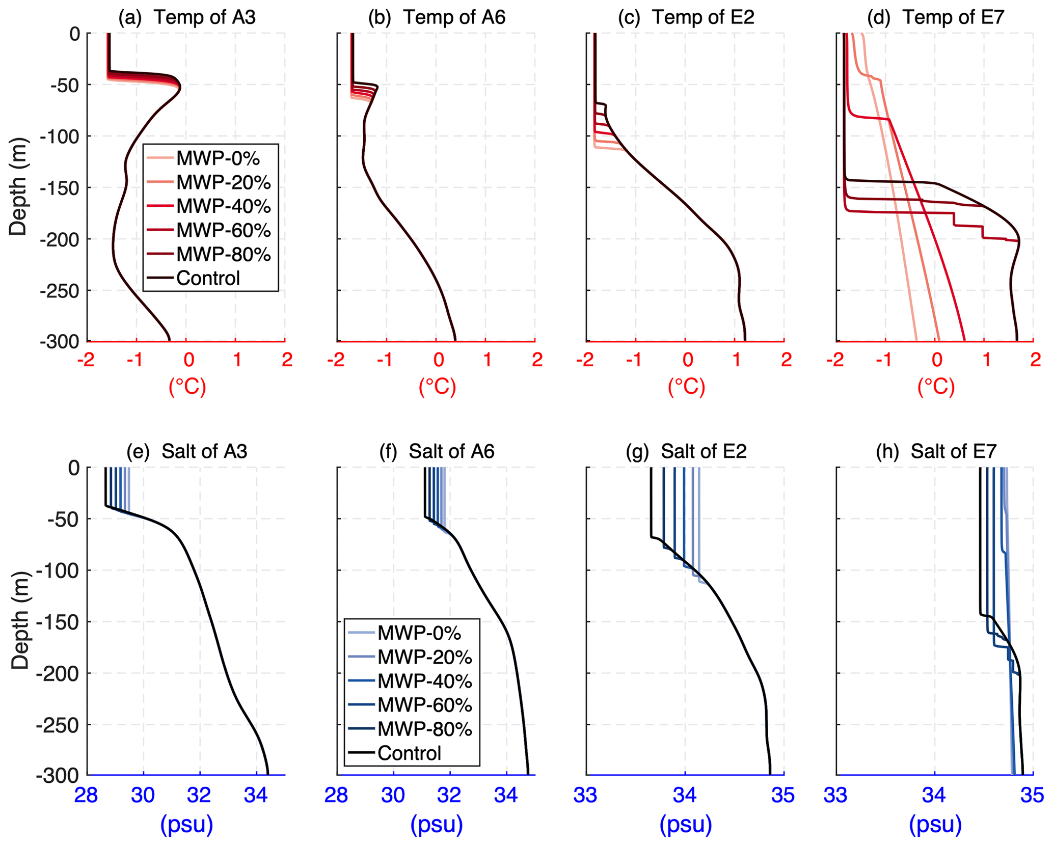
Figure 17 The same as Fig. 11 but for stations A3, A6, E2 and E7 of the thinner initial ice experiments.

4 Discussion

A key finding of this study is that the impact of meltwater on sea ice varies based on the strength of ocean stratification. This suggests that the ice-covered Arctic Ocean can be divided into two regimes based on ocean stratification: some areas with strong stratification that are less sensitive to meltwater, where the meltwater only prevents the NSTM from melting ice, and other small areas with weak stratification that are more sensitive to meltwater, where the meltwater not only prevents NSTM from melting ice in the summer but also prevents warm AW from mixing upward in early spring. The border between these two regimes depends on ocean stratification. Stations E4 and E6 are clear examples. The initial CHL at station E6 is quite weak (Fig. 2f), and the AW is mixed sufficiently upward in the spring after removing the meltwater. Station E4, close to station E6, has a relatively stronger initial CHL than station E6 (Fig. 2f), and the AW cannot reach the upper ocean and ice even when the meltwater is removed.

Wang et al. (2019) noted that although sea ice decline does not change the total Arctic liquid freshwater content (FWC), the increase in the liquid FWC in the Amerasian Basin is nearly compensated for by the reduction in the Eurasian Basin, which results in significant changes in the spatial distribution of the liquid FWC. This raises the question of how the exchange of meltwater between these two regimes in the Arctic Ocean will affect the ocean and sea ice. From our experimental results, it appears that if meltwater or liquid FWC from other sources is continuously lost outwards from an area during the melting season, then the sea ice in that area will melt more rapidly; if this area occurs where the meltwater will have a significant impact, then there is a high probability that the AW will mix sufficiently upward during the freezing season and reach the ice cover, which can cause substantial sea ice melting and prolong the melting season. The warm AW plays an important role in reducing the sea ice cover in the Arctic Ocean through upward heat loss (Polyakov et al., 2010) because the heat contained within the AW layer is sufficient to melt all sea ice in the Arctic within a few years (Turner, 2010). Climate model projections suggest that freshwater input from enhanced river runoff and positive precipitation minus evaporation (P−E) will increase by ∼ 30 % by 2050 (Peterson et al., 2002; Bintanja and Selten, 2014; Haine et al., 2015). Increased freshwater input, like more meltwater entering the ocean, can strengthen the cold halocline by increasing the magnitude of the salinity gradient, which will also inevitably have an impact on sea ice melt and production, especially in some important areas such as stations E6 and E7 in this study.

A limitation of the one-dimensional model is that it cannot directly represent the effect of lateral variations in the upper ocean in combination with ocean/ice advection. But in this study, we focus on the effects of meltwater on vertical processes in the ocean and do not consider the effects of advection, and the simulations are short (1 year). For shorter simulations and relatively horizontally constant temperature and salinity properties, it can be assumed that advection will have a smaller effect (Linders and Björk, 2013). Therefore, the results of the one-dimensional model used in this study can be justified. Advection is of great importance when performing long-term simulations and should be addressed, for example, by introducing some type of restoration of the profiles towards the observed values (Polyakov et al., 2010, 2013b). In addition, as mentioned in Sect. 3.1.2, changes in wind speed will affect stratification and the melt and formation of sea ice through increased vertical mixing. The ideal modeling method used in this study cannot reproduce the episodic high values of ocean–ice heat flux caused by wind mixing, as reported by Jackson et al. (2012) and Smith et al. (2018). Therefore, it is necessary to consider the wind speed with respect to the role of meltwater in the sea ice–ocean coupled system in future work.

This study provides valuable insights into the intricate relationships between ocean stratification, meltwater and sea ice growth and their implications for predicting future changes in the Arctic region. Understanding these complex interactions is essential for developing accurate climate models and assessing the potential impacts of climate change on the Arctic ecosystem. The study in this paper addresses only the effects of meltwater in the vertical direction, and future work could focus on the effects of meltwater transport processes during the melting season in conjunction with Arctic Ocean circulation. To address this issue, more detailed modeling, including advection processes, is needed.

5 Conclusions

In this study, the responses of upper-ocean stratification and sea ice melt and formation in the Arctic Ocean to meltwater release are investigated using a one-dimensional coupled sea ice–ocean model. We perform two types of experiments to achieve the goals of the study: a control run and five meltwater perturbation experiments with 0 %, 20 %, 40 %, 60 % and 80 % meltwater release into the ocean.

Compared with the observations, the one-dimensional coupled sea ice–ocean model reproduces the observed temperature and salinity structure of the Arctic Ocean reasonably well, capturing important features such as the fresh surface layer, the NSTM and the seasonal variation in MLD. In the control runs, the results suggest that ice growth depends on ocean stratification because weaker ocean stratification leads to higher ocean–ice heat flux during winter. In the meltwater perturbation experiments, as expected, decreasing meltwater increases the salinity of the surface and weakens stratification, flattening the upper halocline and changing the vertical heat flux from the depth to the surface. These changes subsequently affect the melting or formation of sea ice. Our results suggest that a decrease in meltwater release has the following effects on sea ice:

1. During the melting season, meltwater has an inhibitory effect on sea ice melt by preventing upward mixing of heat from the subsurface layer. The minimum summer effective sea ice thickness values in the control runs are approximately 17 % greater than those of the MWP 0 % runs, suggesting that the presence of meltwater exerts an inhibitory effect on the process of sea ice melt.

2. During the freezing season, the effect of meltwater released in the previous melting season on sea ice growth varies with ocean stratification. In regions with weaker stratification, such as the Nansen Basin, meltwater plays a more important role in maintaining sea ice and ocean stratification than in areas with stronger stratification, such as the Canada Basin. The model results show that at strongly stratified stations, the net increase in winter effective sea ice thickness in the control run is approximately 12 % smaller than that in the MWP 0 % runs. Conversely, at weakly stratified stations, the net increase in effective sea ice thickness in the control run is approximately 43 % larger than that in the MWP 0 % runs. Our findings reveal that the effects of meltwater from the previous melting season on the subsequent winter ice formation depend on the strength of stratification. Specifically, it impedes ice formation in areas with strong stratification, while it promotes it in areas with weak stratification.

3. Sensitivity experiments with thinner initial ice indicate that as multi-year ice in the Arctic Ocean is gradually replaced by seasonal sea ice, meltwater will play a more significant role in hindering vertical mixing and winter ice melt in the future.