Observations and modeling of tidally generated high-frequency velocity fluctuations downstream of a channel constriction

We investigate data from an acoustic Doppler current profiler deployed in a constricted ocean channel showing a tidally dominated flow with intermittent velocity extrema during outflow from the constriction but not during inflow. A 2D numerical ocean model forced by tides is used to examine the spatial flow structure and underlying dynamical processes. We find that flow-separation eddies generated near the tightest constriction point form a dipole pair which propagates downstream and drives the observed intermittent flow variability. The eddies, which are generated by an along-channel adverse pressure gradient, spin up for some time near the constriction until they develop local low pressures in their centers that are strong enough to modify the background along-channel pressure gradient significantly. When the dipole has propagated some distance away from the constriction, the conditions for flow separation are recovered, and new eddies are formed.

1 Introduction

The flow through ocean channels, or straits, is often fast and associated with nonlinear dynamics – especially when forced by the barotropic tide (Stigebrandt, 1980; Farmer and Freeland, 1983). In such channels, flow-separation eddies can emerge along the channel walls (Kundu et al., 2015). As shown by Wells and van Heijst (2003), tidally generated flow-separation eddies can pair up to form dipoles near the channel exit. These can then self-advect away from the channel, even on the reverse tide. Model studies have shown how these vortex structures have the potential to trap fluid and thus drive significant net tracer transport through a channel (Feng et al., 2019; Nøst and Børve, 2021; Børve et al., 2021). So a good understanding of the nonlinear processes that govern the life cycle and behavior of such vortices is required if one wishes to make accurate estimates of tracer dispersion in a complex coastal zone.

Flow-separation dipoles in the field have been well documented through various drifter and shipboard acoustic Doppler current profiler (ADCP)-based studies (Fujiwara et al., 1994; Old and Vennell, 2001; Whilden et al., 2014). However, analyses of dipole dynamics from fixed observations have received less focus. Easton et al. (2012) present vertically averaged flow observations recorded by an instrument moored downstream from a channel in the Pentland Firth, Scotland. This dataset shows high-frequency flow oscillations on the outflow phase of the tide but, importantly, not on the inflow phase. The authors hypothesize that an unidentified problem with their mooring setup could be the cause of the oscillations, essentially neglecting processes that do not appear to be tidal waves. However, the asymmetry in their mooring response suggests that what they picked up might instead be actual variability caused by flow-separation eddies.

Figure 1 The study domain with the location where we recorded the flow in Tromsøysund marked with a red cross. The right panel zooms in on Tromsøysund with bathymetry shaded and contoured. Background land information has been collected from Cartopy Google Maps tiles (Google, 2021).

The theoretical basis for such eddies originates in a study by Stommel and Farmer (1952), who first approached a dynamical description of oceanic channel flows by noting the distinct asymmetry between a channel's inflow and outflow side. Currents flowing into the channel resemble a potential flow, whereas currents flowing out separate from the channel walls to form a jet. Bernoulli's principle, along with the local effects of side-wall friction, can be used to explain this phenomenon. To conserve the barotropic volume flux through a channel, i.e., to keep $V_{\text{f}}=A\cdot u$ constant, the flow speed (u) must either increase or decrease as the channels' cross-sectional area (A) changes. To do so, some of the fluid's potential energy is converted to kinetic energy as water flows into the channel and speeds up. Conversely, kinetic energy is converted to potential energy as water flows out of the channel and slows down. This results in a dynamic low pressure, i.e., a dip in the sea surface, at the tightest point of the channel and a resultant pressure gradient force directed toward that point from both sides. On the downstream side, the pressure gradient force is thus against the flow direction. When acting in conjunction with side-wall friction, this adverse pressure gradient force may cause some water parcels to stall near the channel walls and even flow back toward the constriction. This situation is known as flow separation, resulting in flow with locally closed streamlines – the flow-separation eddies – and a jet shooting out between these (Kundu et al., 2015).

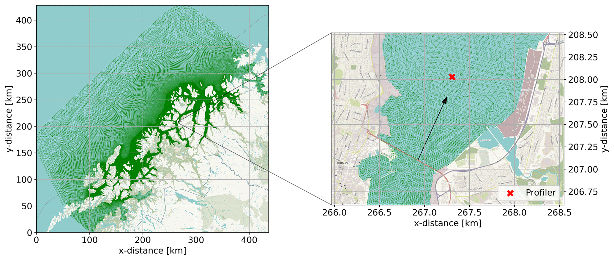
Figure 2 Model mesh. Zoom-in on Tromsøysund to the right. The distances are relative to the domain's westernmost and southernmost extents. The black arrow to the right shows the along-channel direction. Georeference from © OpenStreetMap contributors 2023. Distributed under the Open Data Commons Open Database License (ODbL) v1.0.

Studies exist that have examined the force balance of real channel flows in light of this theoretical framework. Vennell (2006) used a ship-mounted ADCP to argue that the dynamics within a channel were quasi-stationary throughout an entire half tidal cycle (with the flow being in one direction), dominated by the advection of momentum balancing an along-channel pressure gradient force. Their results agree well with Hench et al. (2002) and Hench and Luettich (2003), who, based on model results, argue that the momentum balance is quasi-stationary on ebb and flood on both sides of both an idealized and a realistic channel. Interestingly, Hench et al. (2002) tuned the eddy viscosity in their model and found that weak viscosity excited transient eddies in their simulations. However, they too dismissed these eddies as (model) noise.

The present study offers an alternative interpretation of the noisy signals reported by both Hench et al. (2002) and Easton et al. (2012) by analyzing ADCP data collected from another tidally dominated strait, this one located in Northern Norway. The observations contain a similar high-frequency velocity signal which we can not attribute to instrument errors. The observations are accompanied by high-resolution numerical modeling. We formulate two objectives: (1) to use realistic model simulations to identify flow patterns capable of generating similar current time series to those captured by the ADCP and (2) to use realistic and idealized simulations to investigate the underlying dynamics. The results indicate that the observed high-frequency flow variability is indeed tied to the generation of flow-separation eddies and that the earlier claims of a quasi-stationary force balance must be nuanced.

2 Methods

2.1 Observations

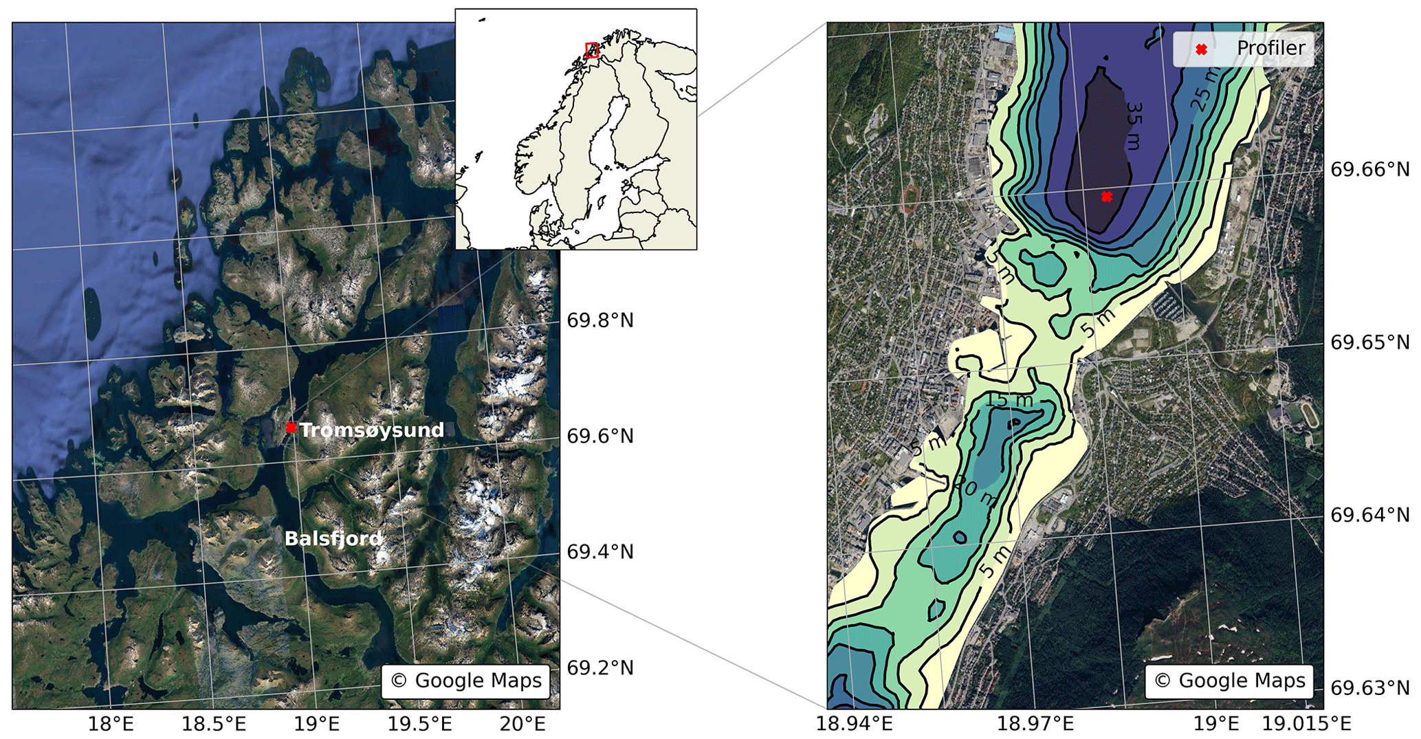
We analyze the flow in the Tromsøysund strait in Northern Norway which connects the 60 km long fjord Balsfjord to the open ocean (see Fig. 1). The observations were collected with an ADCP deployed roughly 1 km north of the narrowest point of the constriction. The instrument was an Aanderaa SeaGuard II, configured to record data for 2.5 min and store averages of these recordings in intervals of 10 min, aiming to reduce the influence of instrument-induced noise and reduce battery consumption. The instrument was deployed in a rigid bottom frame at the end of the winter season, from March to April 2017.

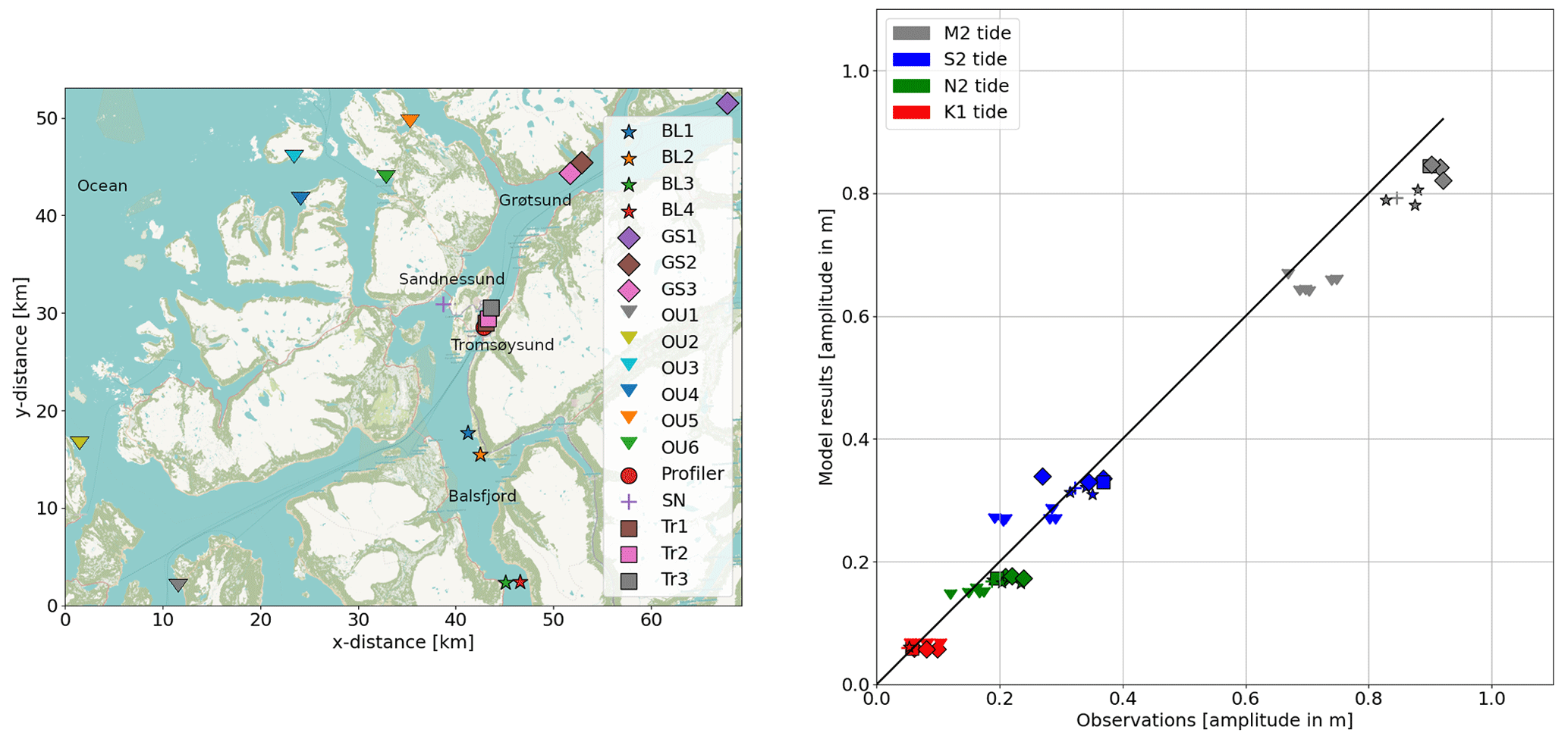
Figure 3 Comparison between tide SSH amplitude of four leading harmonics observations. The left-hand panel shows the moored instruments' position. The mooring stations are labeled by the geographical subdomains they were deployed in: “BL” (from Balsfjord, south of Tromsø), “GS” (from Grøtsundet, north of Tromsø), “Tr” (from Tromsøysund), and “SN” (from Sandnessund). Stations outside of the fjord system are labeled “OU”. The right-hand panel compares the modeled tidal elevation to the observations. Georeference from © OpenStreetMap contributors 2023. Distributed under the Open Data Commons Open Database License (ODbL) v1.0.

Below we will be presenting and discussing the “along-channel” and “across-channel” components of currents, where the along-channel direction is shown with a line in Fig. 2. These two flow components were found by rotating the original east–west (u) and north–south (v) flow components by angle θ between east–west and the along-channel direction as

$$\begin{array}{}\text{(1)}& {\displaystyle }{V}_{\text{along}}=u\cdot \cos \left(\mathit{\theta }\right)+v\cdot \sin \left(\mathit{\theta }\right),\text{(2)}& {\displaystyle }{V}_{\text{across}}=-u\cdot \sin \left(\mathit{\theta }\right)+v\cdot \cos \left(\mathit{\theta }\right).\end{array}$$

2.2 Numerical modeling

We use the Finite Volume Community Ocean Model (FVCOM; Chen et al., 2003). This is a prognostic, free-surface 3D primitive equation ocean model which solves the integral form of the equations on an unstructured triangular horizontal grid. In this study, we use a 2D configuration of FVCOM that solves the depth-averaged momentum and continuity equations for a constant-density fluid. FVCOM calculates momentum advection using a second-order accuracy flux scheme (Chen et al., 2006; Kobayashi et al., 1999). We used a Smagorinsky (1963) closure scheme for the horizontal diffusion of momentum to suppress velocity fluctuations in length scales comparable to the mesh resolution. The Smagorinsky coefficient (C_smag) was tuned by comparing the modeled flow with the observed flow at the ADCP (see below), and the best fit was found when this coefficient was set to 0.2. Furthermore, we used a quadratic bottom friction parametrization: $({\mathit{\tau }}_{\text{b},x},{\mathit{\tau }}_{\text{b},y})={\mathit{\rho }}_{\mathrm{0}}{C}_{\text{d}}\left|\mathbf{\text{u}}\right|\mathbf{\text{u}}$. C_d is calculated using the Chézy–Manning formulation, which is commonly used in coastal ocean circulation models:

$$\begin{array}{}\text{(3)}& C_{\text{d}}=g{\displaystyle \frac{n^{\mathrm{2}}}{\sqrt[\mathrm{3}]{D}}},\end{array}$$

where n is the Manning coefficient, which is n=0.02 in our experiments. We notice from other publications that $n\in [\mathrm{0.013},\mathrm{0.023}]$, with most reported values being in the higher end of the range (see, e.g., Blakely et al., 2022; Lee et al., 2020; Lyu and Zhu, 2018; Mayo et al., 2014; Kerr et al., 2013). Furthermore g is the acceleration of gravity, and D is the water column thickness. The governing equations are integrated in time using a modified explicit fourth-order Runge–Kutta time-stepping scheme (see Chen et al., 2003, for more details). This choice of model physics and parameter settings was used for two tidally forced simulations: one with realistic and one with idealized geometry.

2.2.1 Realistic simulation

We used the mesh generator DistMesh (Persson and Strang, 2004) to create a mesh focused on Tromsøysund, consisting of 747 761 triangles (cells) and 393 422 triangle corners (nodes). The resolution varied from 13 m in Tromsøysund to 8 km at the open boundary (see Fig. 2). The domain was bounded by land defined by coastline polygons obtained from the Norwegian Mapping Authority (Kartverket, 2022). The smallest triangle angle in the domain was 30^∘, and the largest was 117^∘. No triangles had more than one side facing the model boundary. The bathymetry was also retrieved from the Norwegian Mapping Authority high-resolution bottom bathymetry database.

The model was forced with sea surface height (SSH) data of 13 tidal harmonics (M2, S2, N2, K2, K1, O1, P1, Q1, Mf, Mm, M4, MS4, MN4) extracted from TPXO7.2 (Egbert and Erofeeva, 2002) and interpolated to the open boundaries. We used TPXO7.2 since the modeled current in Tromsøysund compared better with the observations when using this dataset to force the open boundary than when using the newer TPXO9-atlas-v5. FVCOM computes velocities at the open boundary using a reduced set of Chen et al. (2003). We ramped the model up from rest and a flat sea surface to full forcing over 30 d.

To assess the models performance, we compared its results to sea surface elevation measurements from 18 mooring stations in the Tromsø region. The moorings were made up of a mixture of point measurement devices (Aanderaa RCM) and ADCPs (Aanderaa SeaGuard II and Nortek Aquadopp); all were fitted with pressure sensors that operated for 1–2 months to cover two or more spring–neap cycles. Figure 3 shows the mooring locations and a scatter plot of the observed and modeled SSH amplitude of M2, S2, N2, and K1 tidal constituents. These were calculated with the UTide harmonic analysis software (Codiga, 2011).

Figure 4 Idealized model mesh with shaded bathymetry as background.

The semi-diurnal constituent (M2, S2, N2) amplitudes increase going northward and are an order of magnitude bigger than the diurnal constituent (K1); this is consistent with findings by Gjevik et al. (1994). The modeled M2 amplitude is slightly underestimated, which may indicate the M2 amplitude is too small at the model's open boundary. However, the model captures the spatial spread of the M2 amplitude well.

The spatial spread of the other constituent's amplitude is smaller in the model than in the observations. We do not know why this is the case, and we can not rule out a problem with the model's ability to capture the minor constituent's regional variability. But it is also possible that the observed spread is overestimated. The instruments were deployed on a mooring line, so any vertical movement of the rig in response to the tidal current applying torque to the rig would amplify the observed pressure oscillations and influence the harmonic analysis. It is also possible that while the rigs were deployed sufficiently long to get a good estimate of the leading harmonic (M2), the deployment period was insufficient to get a good spectral estimate for the minor components. As the minor components are much weaker than the M2 tide, they are more susceptible to noise.

This study examines the tidal current driven by a local sea surface elevation difference along the Tromsøysund channel. The model-predicted amplitudes are close to what was observed, and the scatter around the one-to-one line is low, so we therefore think Fig. 3 serves as an indication that the model represents tidal variability in the region sufficiently well to develop the tidal jet at the Tromsøysund constriction.

2.2.2 Idealized simulation

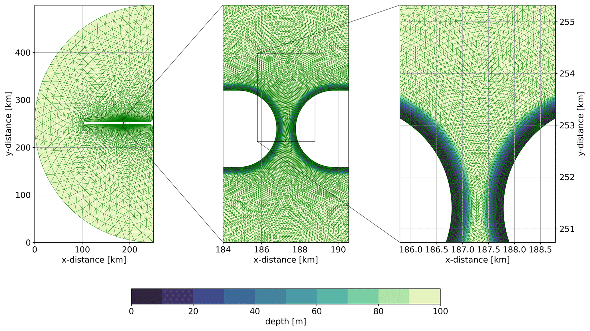
To help isolate the key dynamics in a more idealized setting, we used the same FVCOM channel setup as in Nøst and Børve (2021). The domain is shown in Fig. 4 and consists of a 1 km wide channel which cuts through a peninsula. The channel has a maximum depth of 100 m deep in its center and is 5 m deep near the side walls. The model is forced at the open boundary with a semi-diurnal tidal wave with an SSH amplitude of 10 cm, and velocities at the boundary are again calculated by the reduced physics algorithm as used in the realistic simulation.

3 Results

3.1 Observed and modeled flow in Tromsøysund

The currents in Tromsøysund, measured by the ADCP at all depth levels over approximately three diurnal tidal cycles during spring tide are shown in Fig. 5. The velocity components have been rotated, as described above, so what we see here is the flow approximately in the along-channel direction. Positive values indicate flow out of the constriction (predominantly northward), whereas negative values are into the constriction (southward). A semi-diurnal signal dominates the time series, but the flow is asymmetric, being stronger on outflow than inflow. In addition, the record reveals high-frequency variability, which appears to be more predominant on outflow than inflow. Finally, both the tidal signal and the high-frequency variability are predominantly barotropic, lending strong support to the idea of treating the flow as 2D in the model simulations.

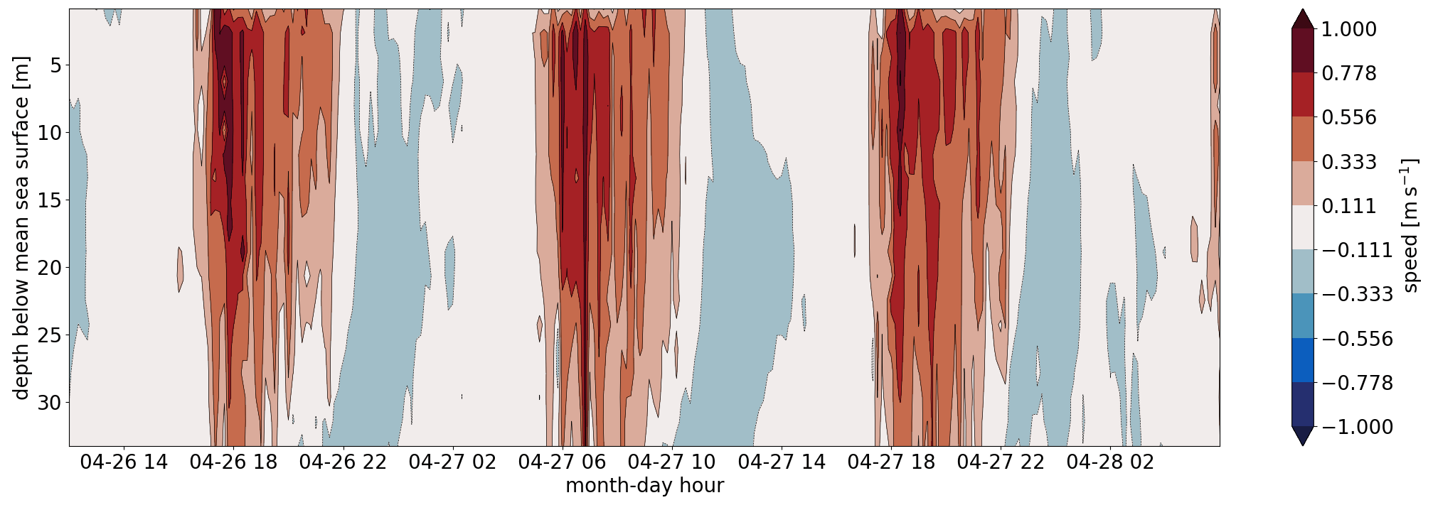
Figure 5 The along-channel flow component as a function of time and depth, as measured by the ADCP instrument in Tromsøysund.

Figure 6 shows the observed velocity both in the along-channel (left panel) and across-channel (right panel) directions, now after depth-averaging, so positive values here indicate flow with predominantly northerly and easterly components, respectively. Each reading is indicated with a red dot. In addition, a blue line indicates the pure tidal components of the flow, reconstructed using the UTide tidal harmonic analysis package (Codiga, 2011). We now see even more clearly how the along-channel flow (left panel) is asymmetric, being stronger on outflow than on inflow. The harmonic analysis picks up the asymmetry at tidal frequencies and reproduces the southward flow (inflow). But on northward flow – from the constriction and toward the ADCP – the observations show high-frequency velocity spikes of about 20 cm s⁻¹ superimposed on the tidal signal. The fact that these are systematically observed on only northward tidal flow suggests that they are associated with tides rather than, e.g., atmospheric fluctuations. But being very high frequency, the harmonic analysis does not capture them.

The across-channel (right panel) flow pattern is similar to the along-channel flow in that the harmonic analysis captures the dynamics extremely well on the southward but not on the northward tide. Notably, whereas the tidal signal is strongest in the along-channel direction, the high-frequency variability is fairly isotropic. Thus, we will subsequently focus on the high-frequency velocity fluctuations in the along-channel direction when comparing them with the model results below.

Figure 7 compares the model and observations for the same three semi-diurnal tidal cycles. The depth-averaged along-channel flow component is shown in the left panel, while SSH is shown in the right panel. The numerical model captures the along-channel flow asymmetry well, including a clear predominance of high-frequency spikes on the outflowing phase of the tide. In this simulation, the amplitude of the spikes is generally somewhat higher than in the observations, but this can partially be tuned by the choice of model bottom friction and viscosity parameters (see Discussion). The modeled sea surface elevation signal also tracks the observations fairly well, as suggested by the more broad comparison shown in Fig. 3, even if small amplitude and phase offsets can be detected.

Encouraged by the model–observation comparisons, we look at model fields in more detail to investigate the source of the high-frequency fluctuations. Figure 8 shows the model flow field in Tromsøysund for nine time snapshots on 26 April 2017 (the period is indicated by dark gray in Fig. 7). The bottom panel of the figure shows a time series of the along-channel flow extracted from the nearest mesh triangle to the ADCP (indicated with a white star in the above nine snapshot panels).

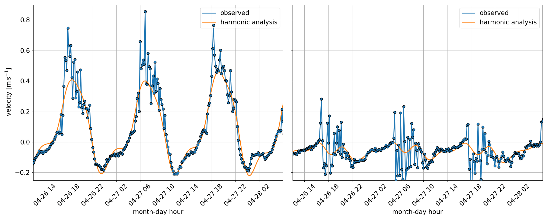
Figure 6 Depth-averaged velocity components in along-channel (approximately northerly) and across-channel (easterly) directions, as measured by the ADCP. Dots indicate each actual observation. Blue lines are reproductions of the tidal contribution based on harmonic analysis.

Panel a, taken only a few minutes after the tide has started to flow northward, shows that two flow-separation eddies have already formed just downstream of the constriction. Panel b shows the situation 15 min later when the eddies have intensified. They have now detached from their generation site and started to move downstream. The combined velocity field of the dipole pair concentrates and guides the jet in between them. Another 15 min later, in panel c (+30 min), the dipole has moved further downstream, and the left-hand eddy, which rotates counterclockwise, has begun to influence the strength and direction of currents where the ADCP is located. As this left-hand eddy passes just to the right of the ADCP, it reverses the currents sampled at this location, as also seen in panel d (at +40 min and as outlined in the lower time-series panel). During this period and, in fact, throughout the remaining panels, the right-hand eddy is fairly stationary, appearing to be trapped by features in the coastline.

The initial dipole pair is particularly strong and noticeable. But a series of secondary eddies also forms as soon as the initial pair has left the generation site. In particular, a string of new counterclockwise eddies forms on the left-hand side, captured in panels c, e, and g. These, in turn, also propagate towards and past the ADCP, impacting the flow recorded by the fixed instrument there. At least one new clockwise eddy can also be seen spinning up on the right side of the channel in panels g to i.

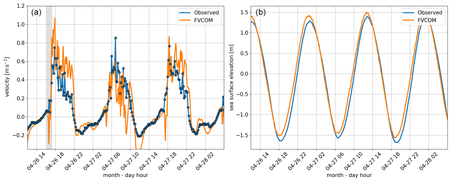
Figure 7 Observed and modeled along-channel velocity (a) and sea surface elevation (b) 26 April 2017 at 12:00 UTC to 29 April 2017 at 12:00 UTC. Gray shade indicates the time period studied in detail in Fig. 8.

A key take-home message from Fig. 8 is that the high-frequency variability recorded by the ADCP instrument in Tromsøysund reflects the chaotic flow related to the flow-separation eddies and jet. The jet is concentrated between eddy dipole pairs, and its strength can be comparable to the flow in the narrowest part of the constriction itself. Multiple secondary eddies can form after the initial dipole detaches, and the relative positioning of the eddies, both primary and secondary, decides how the jet meanders. Details of the channel geometry have a large impact, and in Tromsøysund, eddies forming along the right side are partially trapped by the coastline shape. In contrast, eddies to the left easily propagate down the channel.

A second point to note is that the observed progression of events from primary eddy formation via detachment and dipole advection to the generation of secondary eddies suggests that the dynamical balances in the constriction may not be as stationary through the outflow period as suggested in the published literature (by e.g., Vennell, 2006; Hench et al., 2002; Hench and Luettich, 2003). To examine the underlying dynamics in more detail, we therefore proceed to take a look at the along-channel pressure field. To help isolate the relevant dynamics, we first turn to the simulations of flow in the much more idealized channel geometry.

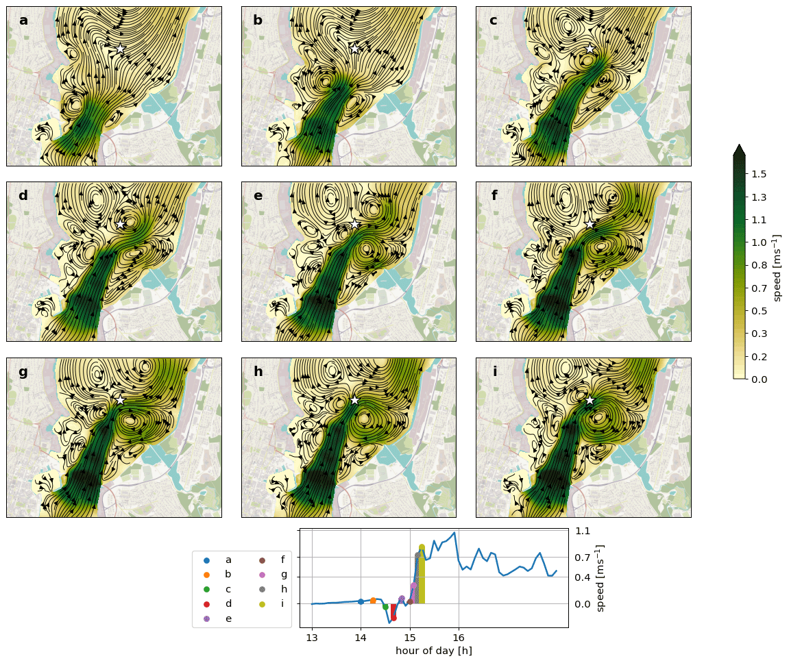
Figure 8 Snapshots of the flow in Tromsøysund, showing streamlines and flow speed (color). Panel (a) is from 16:00 UTC on 26 April. Relative to (a), (b) is +15 min, (c) is +30 min, (d) is +40 min, (e) is +50 min, (e) is +1 h, (g) is +1 h 5 min, (h) is +1 h 10 min, and (i) is +1 h 15 min. The lower panel shows a time series of the along-channel flow at the grid location closest to the ADCP (white star). Dots and bars of different colors indicate when the snapshots in the top nine panels were taken. Georeferences from © OpenStreetMap contributors 2023. Distributed under the Open Data Commons Open Database License (ODbL) v1.0.

3.2 Dynamical evolution

Figure 9 shows snapshots of the flow field from an outflowing tide in the idealized run. The flow is initially similar to a Bernoulli flow (panel a). The streamlines converge on the inflow side, the maximum speed is in the center of the channel, and streamlines diverge on the outflow side. A large counterclockwise eddy downstream of the constriction is a remnant from an earlier tidal cycle. Panel b, taken 1 h later (+1 h), then shows the flow state shortly after flow separation, and we see that eddies have formed on both sides of the channel, similar to the initial dipole in Tromsøysund. This dipole pair modifies the flow by concentrating it in a narrow band – the jet – exiting the channel. In panel c (+2 h), the dipole has pinched off the constriction and begun to move downstream. It continues to propagate away from the channel in subsequent time slices. Panel d (+2 h 30 min) then shows that a secondary eddy develops to the right in the channel after the dipole has left. New eddies can also form in panels f and g (at +3 h 30 min and 4 h), so the development of both primary and secondary eddies and dipoles are also captured in this simulation. Again, we see that the jet strength, especially when guided between a dipole pair, is comparable and can even surpass the flow strength in the narrowest part of the constriction itself.

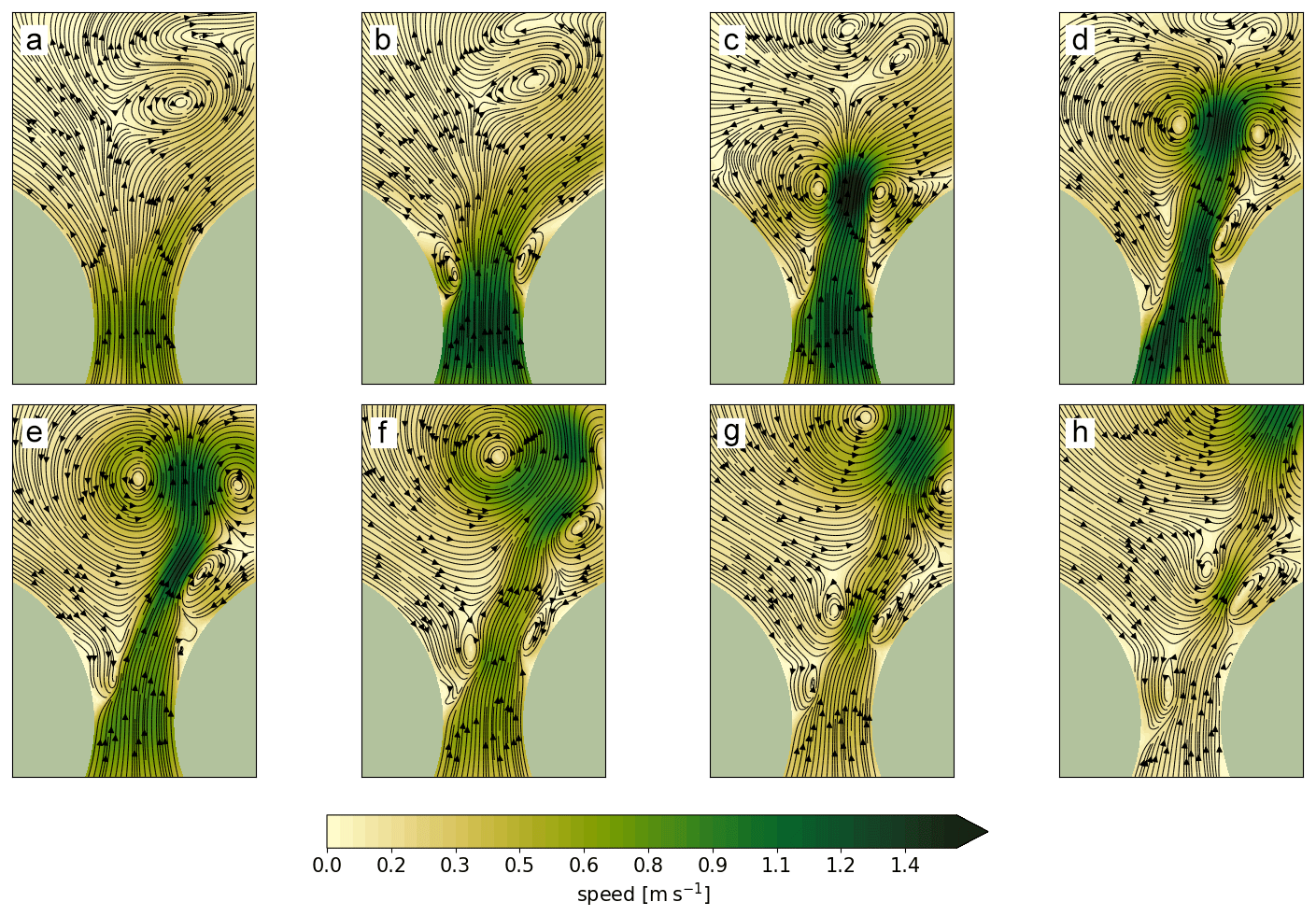
Figure 9 Flow field evolution in the idealized channel run. Relative to (a), (b) is +1 h, (c) is +2 h, (d) is +2 h 30 min, (e) is +3 h, (f) is +3 h 30 min, (g) is +4 h, and (h) is +4 h 30 min.

As the dipole guides the jet, it is not entirely obvious how to separate the two, so one can also say that the flow speed associated with the dipoles themselves is comparable in strength to the speed at the constriction in both the idealized and realistic simulations. This suggests that the pressure perturbations associated with those eddies may also be comparable to the channel-scale dynamic pressure – and adverse pressure gradient – which causes flow separation in the first place. We now look for evidence of this by examining how the pressure field (SSH) near the constriction changes in response to the presence of eddies.

Figure 10 shows the along-channel pressure gradient force with streamlines plotted on top. Red and blue colors here indicate a pressure force up and down the channel, respectively. The time interval is somewhat shorter than in Fig. 9 as we now wish to examine the dynamics around the initial dipole pair primarily. Panel a again shows the situation just after slack water, when a weak large-scale positive pressure gradient has started to accelerate the fluid through the channel. At this early time, the local dynamic pressure gradient is weaker than the large-scale gradient that actually drives the flow. Panel b shows the state 30 min later (+30 min). An adverse pressure gradient has formed and acts to decelerate the flow on the outflow side of the channel, and there is already some sign of flow separation building up near the left channel wall. In panel c, at +1 h, two distinct eddies have formed, one on either side of the channel. Being in cyclostrophic balance, their along-channel pressure gradient signals are adverse on the downstream flank but favorable (in the direction of the large-scale forcing) on the upstream flank. In panel d, at +1 h 15 min and after the eddies have grown in size and strength, the eddy pressure anomalies influence the larger-scale adverse pressure gradient around the channel exit considerably, reversing its sign near the walls. The two vortices still spin up at the location of their generation at this stage. But after another 15 min, in panel e (+1 h 30 min), the eddies detached from the sidewalls and started to approach each other. The favorable pressure gradient force tied to the dipole extends across the entire channel width. It is after this time that the dipole pair begins to translate and leave the constriction (panels f–h). Importantly, as the primary dipole pair have traveled slightly downstream, a distance amounting approximately to their diameter, the background adverse pressure gradient again dominates near the channel constriction. In panel g (+2 h 30 min), a secondary eddy has formed along the right-hand wall (corresponding to panel d in Fig. 9). This new eddy then commences traveling downstream in panel h (+3 h 15 min).

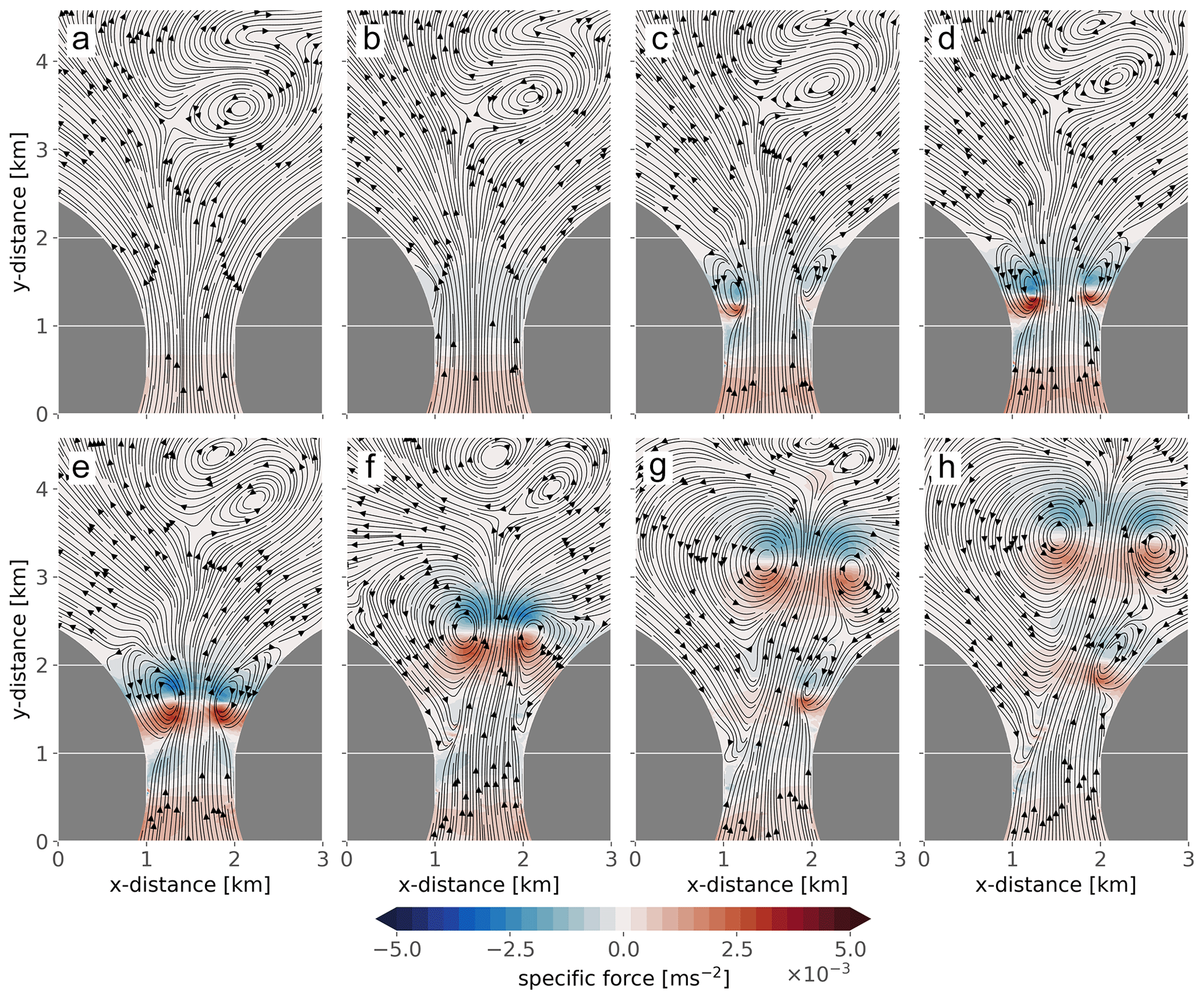
Figure 10 Along-channel pressure gradient during eddy growth. Relative to (a), (b) is +30 min, (c) +1 h, (d) 1 h 15 min, (e) +1 h 30 min, (f) +2 h, (g) +2 h 30 min, and (h) is +3 h 15 min.

So Fig. 10 suggests that the initial vortex pair detaches from the generation region when its pressure anomalies can locally cancel the adverse pressure gradient across the channel width. To examine this relationship, we form a time series of the along-channel pressure gradient and along-channel velocity, now averaged over a transect which crosses the channel approximately where the vortices originally form. Figure 11 shows the result. A little more than two tidal cycles are shown, and gray shading indicates the period corresponding to Fig. 10. When interpreting the time series, it is worth noting that the pressure gradient force here (as well as in Fig. 10) is the total force, which includes (i) the large-scale background pressure force due to the imposed tidal wave, (ii) the dynamic force which reflects the exchange between potential and kinetic energy along the channel, and (iii) the force anomalies due to the eddies.

The cross-channel-averaged pressure gradient force is directed toward the constriction (negative) on southward flow, as expected as both the large-scale tidal and the channel-scale dynamic pressure gradients point in the same direction. The velocity signal is then smooth, acting as a potential flow, as seen explicitly in the fields. Around the subsequent slack water, there is a brief period when the large-scale forcing dominates and sets up a pressure gradient force out of the constriction (positive). But the local dynamic pressure soon dominates and establishes an adverse pressure gradient against the large-scale flow through the channel. Around this time, the cross-channel-averaged velocity decreases, reflecting reverse flow associated with the spin-up of the primary dipole pair. Note that the reduced cross-channel-averaged velocity does not need to imply a reduced total volume flow since the reverse flow occurs near the channel walls where the depth is reduced. Then a sharp reversal in pressure gradient follows, a spike, which coincides with an increase in the averaged flow speed. The abrupt transition reflects the detachment and propagation of the initial vortex pair away from the generation region – and the transect. Subsequent noise in both pressure force and velocity signals presumably reflects secondary eddy formation, detachment, and propagation.

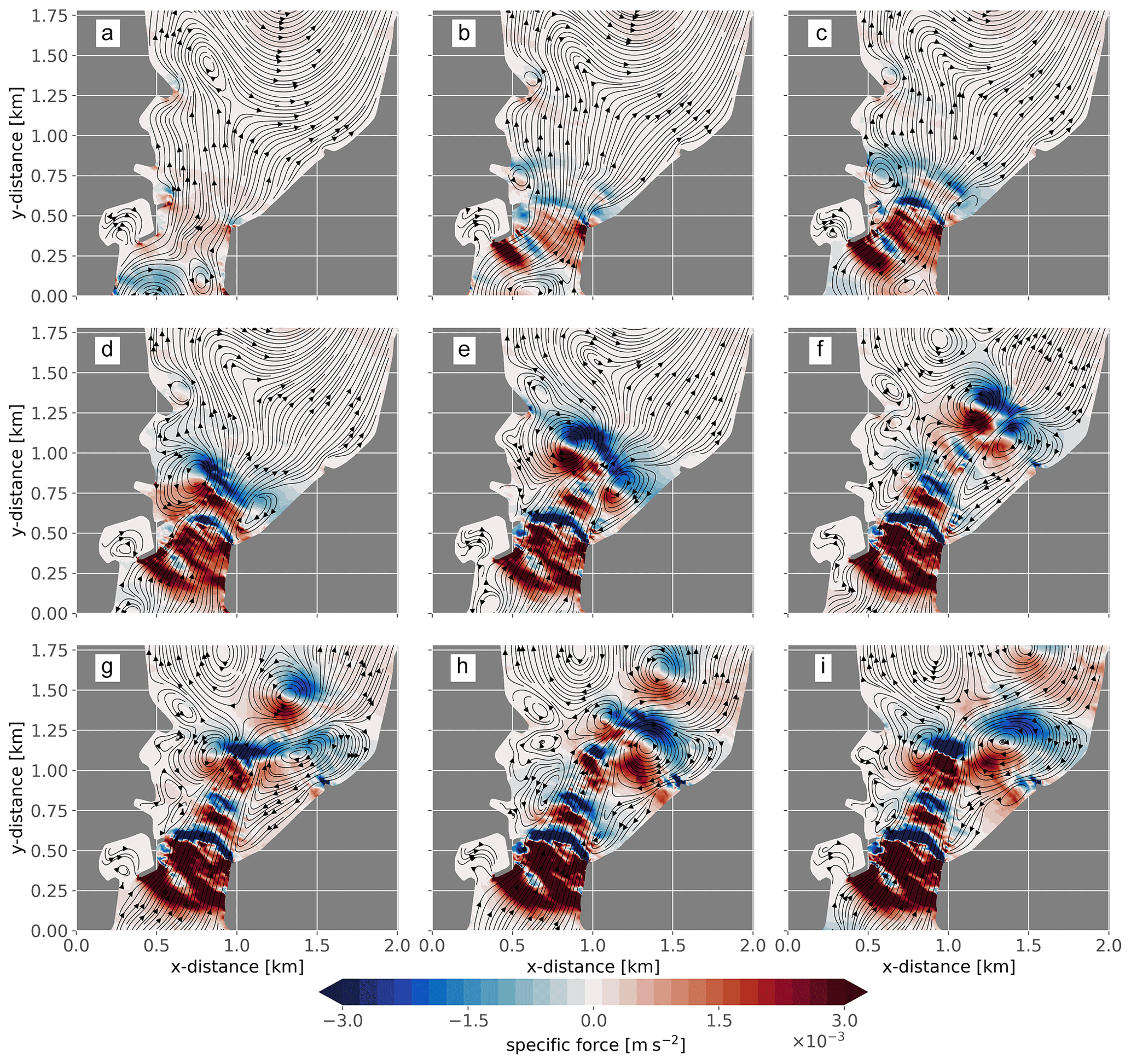
The results thus indicate that the model never reaches a quasi-steady adverse pressure gradient force during outflow conditions due to the dynamic signals imposed by both primary and secondary flow-separation eddies. We now return to Tromsøysund to see if the same force pattern can be found there. Snapshots of the along-channel pressure gradient force and streamlines there from the realistic simulation are shown in Fig. 12. The panels are taken from the same tidal cycle as in Fig. 8 but now again focus on the period around the initial dipole pair. Panel a shows the situation just after slack tide. The along-channel pressure gradient downstream of the narrowest point of the channel is positive, reflecting the large-scale pressure gradient driving the tidal signal. The streamlines at this point in time suggest potential flow. A region of reversed pressure gradient southward of the narrowest constriction is the dynamic imprint of an older vortex situated there. A total of 20 min later (panel b, +20 min), the flow strength through the channel has increased, and the pressure gradient force downstream from the channel center has turned adverse. But the streamlines still mostly follow the channel except near the first flow-separation eddy, which has formed along the left boundary. At +30 min (panel c), the pressure gradient force is strongly adverse where the channel expands, and a flow-separation eddy has also formed on the right side. At +40 min (panel d), the dynamic pressure signal from the two eddies extends across the channel, creating a favorable gradient in their wake. At this point, the counterclockwise vortex to the left starts to move downstream. The remaining panels show a complex pressure force pattern which is harder to interpret. But between +55 min and +1 h 5 min (panels e and f), we observe a recovery of a strong adverse pressure gradient and the generation of a secondary eddy on the left-hand side. After this time, more secondary eddies form, at least on the left side. These then appear to be associated with the development of alternating bands of favorable and adverse pressure gradients along the jet path.

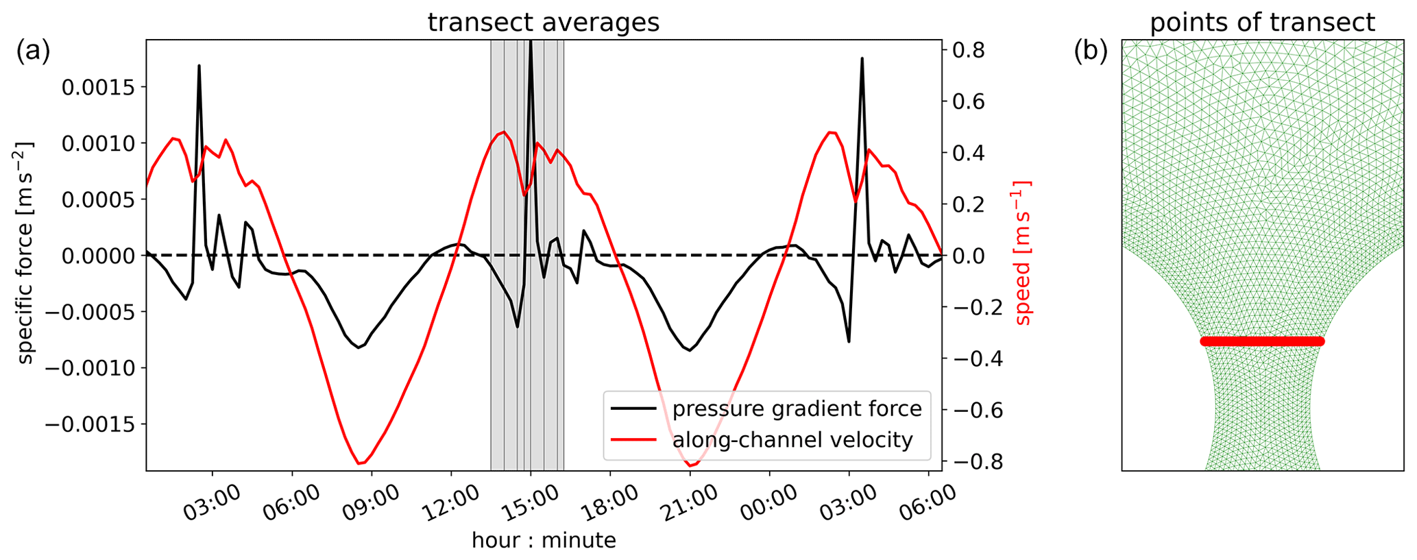
Figure 11 (a) Across-channel-averaged along-channel pressure gradient (black line) and along-channel velocity (red line). The dark shaded area indicates the time span of panels shown in Fig. 10. The vertical gray lines indicate values for each panel in Fig. 10. The dashed line indicates the zero level. (b) Red dots illustrate that the transect was extracted from a location downstream from where the channel expands. The absolute time here is arbitrary.

Finally, as for the idealized channel, we average fields across the strait, approximately where flow separation occurs. Figure 13 shows the resulting time series of along-channel pressure gradient force and velocity. These averaged fields are also noisier than the corresponding fields extracted from the idealized channel run, but a few key features seen earlier can be recognized. On southward flow, when the large-scale forcing and dynamic Bernoulli response have the same signs, the total pressure signal is fairly smooth, reflecting potential flow. After slack tide, at the very beginning of northward flow, the net force tends toward negative values – towards the constriction – as the flow speed increases. But then comes a very strong positive, i.e., favorable, pressure force spike. This behavior on outflow, the build-up of an adverse pressure gradient interrupted by a favorable pressure gradient spike, is seen in all the shown cycles. The spike is not, however, associated with the concurrent reduction in flow speed that we saw in the idealized case. The difference here, we speculate, is tied to the volume conservation constraint and, by implication, details in the bottom topography profile across the channel. After the initial spike, the channel pressure force fluctuates noisily between positive and negative values, as suggested by the later snapshots of Fig. 12. So, despite the increased noise, it is clear that an adverse pressure gradient is not stably present throughout the outflow phase of the tide.

4 Discussion

4.1 Pressure gradient at the entrance

Figure 14 outlines what we believe are the fundamental features of the dynamical fields studied above. The left panel shows a fictitious sub-critical and inviscid Bernoulli flow through a constricted channel. Here, the sea surface dips at the center of the constriction due to the conversion from potential to kinetic energy. On top of this nonlinear response is a large-scale pressure gradient which drives the flow in the first place (not shown). However, the smooth potential flow shown in the left panel is unattainable when accounting for side-wall friction. In reality, friction and the adverse pressure gradient force downstream of the constriction work against the flow, and the flow will separate from the side walls (Kundu et al., 2015). The separation generates circular motions – eddies – on both sides of the constriction, as shown in the right panel.

As the cyclostrophic eddies spin up, low-pressure anomalies develop in their centers. Our model results indicate that the eddies pinch off the constriction when the eddy-induced pressure anomalies are strong enough to change the direction of the pressure gradient around the position where the flow is separated initially. Once the direction of the pressure gradient force is reversed locally, the conditions which caused flow separation in the first place have been violated. The eddies then detach from the walls and translate down the channel, either advected by the jet or self-advecting as a dipole (see below).

Figure 12 Along-channel pressure gradient. Relative to (a), (b) is +20 min, (c) is +30 min, (d) is +40 min, (e) is +55 min, (f) is +1 h 5 min, (g) is +1 h 15 min, (h) is +1 h 25 min, and (i) is +1 h 35 min. Panels (e) and (f) correspond to (b) and (c) in Fig. 8.

4.2 Implication for startup and dipole velocity

Our interpretation of the model results above may offer an alternative view into two closely related topics related to flow-separation dipoles, namely startup time and dipole velocity. The startup time, as defined by Afanasyev (2006), is the time between initial vortex formation and the moment when the dipole starts translating. Earlier scaling arguments have focused on the build-up of sufficient vorticity in the eddies, while here, we argue that the dipole starts translating when the eddy pressure field is strong enough to dominate across the strait in such a way that the necessary conditions for flow separation are removed. Thus, the evolution of the eddy pressure field determines the startup time. Thus, we suggest that the vorticity and pressure descriptions should be complementary. Simply put, since the eddies are in cyclostrophic balance, their vorticity and pressure fields are tightly connected. Therefore, an eddy building up its vorticity, fed by the strong vorticity front created by flow separation, will also have a pressure field that builds up. The added value of the pressure analysis used here is the connection to the dynamic pressure gradient force, which controls flow separation in the first place.

Thus, as we have seen, when the dipole moves away from the strait, flow-separation conditions are restored, leading to the formation of the next dipole pair. Hence, multiple dipole pairs can form over one half tidal cycle. The time between new dipole pairs or, alternatively, the frequency of dipole formation should be determined by the startup time plus the time it takes for a dipole to move a distance sufficient for the flow-separation conditions to be restored. This distance is likely related to the vortex diameter, and the translation timescale then depends on the vortex size and the dipole translation velocity.

But are dipoles in a tidal strait advected passively by the jet after detaching or do they self-advect? Afanasyev (2006) found that dipoles formed in the laboratory moved with a speed equal to half the jet velocity U_max. Nøst and Børve (2021), having simulated and studied flow in several ideal tidal straits of different geometries, found that flow-separation dipoles moved with a velocity $U_{\text{dip}}=(a/b)U_{\text{max}}$, where a is the eddy core radius and b is the core separation distance. Assuming, for simplicity, a jet which increases linearly from zero at the channel walls to U_max in the center, the results of Afanasyev (2006) and Nøst and Børve (2021) thus agree for vortices that each have a diameter which is half the channel width. However, Nøst and Børve (2021) also found that the same dipoles followed

$$\begin{array}{}\text{(4)}& U_{\text{dip}}={\displaystyle \frac{\left|{\mathrm{\Gamma }}_{\mathrm{1}}\right|+\left|{\mathrm{\Gamma }}_{\mathrm{2}}\right|}{\mathrm{2}\mathit{\pi }b}},\end{array}$$

where $\left|{\mathrm{\Gamma }}_{\mathrm{1}}\right|$ and $\left|{\mathrm{\Gamma }}_{\mathrm{2}}\right|$ are the magnitudes of the circulation in each of the two eddies. The expression, incidentally, is twice that which is traditionally used to describe the self-advection velocity of two identical point vortices (of opposite sign) in an otherwise still fluid (Kundu et al., 2015). This dual finding by Nøst and Børve (2021) naturally points to the fact that the jet strength gives the eddy strength. In fact, assuming point vortices of equal strength, each having vorticity which scales as $U_{\text{max}}/a$, gives circulation Γ=πU_maxa (after applying Green's theorem) and a self-advection velocity $U_{\text{dip}}=(a/b)U_{\text{max}}$, i.e., the same as if assuming passive advection by the mean jet. This result indicates that the jet and the eddies are tightly connected and should probably not be studied in isolation. We will not dive into a further quantification of these relationships here but only point back to Figs. 8 and 9, which show how the jet itself is also “stretched” by the dipoles, following their track away from the constriction.

4.3 Variable pressure gradient force at the exit

The observed dynamical behavior on the downstream side of the constriction deviates significantly from what was reported by Hench et al. (2002) and Vennell (2006). In our results, we find a quasi-stationary pressure-gradient force directed toward the constriction on the upstream side, as did the cited studies. But the pressure gradient is non-stationary on the downstream side due to the strong pressure fluctuations associated with the eddies. These oscillations vary over several minutes and may easily pass undetected by a point observation from the field if the data are smoothed over long intervals. They may also be “undetected” in a numerical model if the eddy viscosity used is too high. Our interpretation is, however, in agreement with results reported by Nicolau del Roure et al. (2009), who studied the development of eddy dipoles in the laboratory. They concluded that dipoles developed for some time close to the constriction before, as they put it, being entrained by the jet and subsequently advected downstream. Here we have also found indications that the same chain of events repeats to produce a set of secondary eddies and that the combined effect is a strong and chaotic flow field downstream of the constriction.

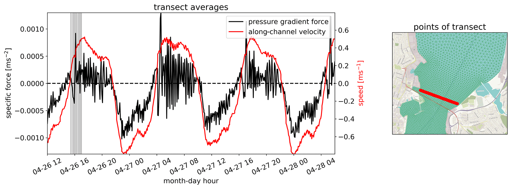
Figure 13 (a) Same calculation as in Fig. 11. Across-channel-averaged along-channel pressure gradient force in Tromsøysund. The gray shading indicates the time span of all panels in Fig. 12, and each vertical line indicates each individual panel. The dashed line indicates the zero level. Right panel: positions used to compute the transect. Georeference from © OpenStreetMap contributors 2023. Distributed under the Open Data Commons Open Database License (ODbL) v1.0.

4.4 Limitations of this work

Shallow and narrow channels with strong tidally driven currents are often well mixed. In addition, wind work and convective mixing add to weak density stratification, especially during late winter at high latitudes (Sælen, 1950). Indeed, the ADCP in Tromsøysund revealed a barotropic tidal flow here, motivating the use of the 2D modeling approach. This somewhat simplistic modeling approach was computationally inexpensive (compared to a 3D approach). However, the results fit well with the observations, indicating that we captured the dominating physical mechanisms in this channel. We therefore chose not to pursue more complex modeling approaches (e.g., 3D), forcing mechanisms other than the tide or dynamics influenced by stratification. However, we note that neither our observations nor model results are necessarily well-suited to assess the dynamical evolution when freshwater input from rivers is more substantial in late spring, summer, and fall. Such situations should be investigated with a 3D approach where impacts of stratification can be included. For example, a strongly stable density stratification may allow the barotropic tide to excite internal gravity waves, which can then radiate energy far away from the constriction (as discussed by, e.g., Inall et al., 2004). Another interesting path to pursue in future work would be to check to what extent internal pressure gradients due to internal hydraulic phenomena can influence the total along-channel pressure gradient and – consequently – the process described herein.

A full 2D approach can even be questioned for a completely barotropic fluid, as non-hydrostatic vertical motions, neglected here, can be significant given sufficiently small scales and strong currents (Albagnac et al., 2014; van Heijst, 2014). Furthermore, in a full 3D setting, the water parcels closer to the bottom will be attenuated more, resulting in upwelling in the eddies' core. In short, it is conceivable that our simplified approach has ignored 3D effects that influence the eddy dynamics even during wintertime. However, to what extent such 3D effects are relevant in the early stages studied herein and when flow separation occurs and the eddies start to grow are, to the best of our knowledge, not known.

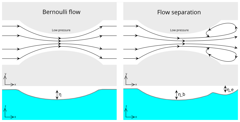
Figure 14 Sketch of streamlines and sea surface perturbation in a pure Bernoulli flow and with flow separation and eddies downstream.

In this study, we chose to use a depth-dependent drag coefficient. This parametrization will introduce a horizontal shear stress, which can assist in the buildup of the headland eddies. However, while the bottom roughness coefficient varies with depth (D) as $C_{\text{d}}\propto \mathrm{1}/\sqrt[\mathrm{3}]{D}$, the bottom friction, as formulated in the shallow-water equations, is also depth-dependent: $F\propto C_{\text{d}}/D$. The depth dependence of bottom friction is thus not dominated by the choice of drag coefficient. Therefore, it is expected that the formation of flow-separation eddies downstream of channel constrictions in ocean models is far less dependent on the parametrization of bottom friction than on horizontal momentum diffusivity.

As described in the model setup, we tuned the Smagorinsky mixing coefficient to obtain model results that fit well with the observations. By increasing or decreasing this parameter, the model results changed somewhat. From the idealized results, it may be tempting to conclude that the first dipole will always be stronger than the subsequent ones. However, in simulations where we tested with stronger forcing and weaker horizontal viscosity (smaller Smagorinsky coefficient), we found that the subsequent dipoles can approach the magnitude of the initial dipole. We can, therefore, not categorically state that the secondary eddies are weaker than the first every single tidal cycle. But, more generally, applying higher eddy viscosity resulted in a flow with weaker nonlinearity and eddy production, producing velocity signals of lower frequency on the downstream side of the constriction. This is, of course, not unexpected and only serves to highlight the point that the high-frequency variability observed in Tromsøysund is inherently due to nonlinear dynamics.

5 Conclusions

A high-resolution low-viscosity numerical ocean model has been used to interpret high-frequency barotropic velocity fluctuations observed by an ADCP downstream of a channel constriction in Northern Norway. The simulations showed that the fluctuations, which exist only on the outflowing tidal phase, reflect flow-separation eddies that pinch off the channel walls and propagate downstream. These eddies, which may form a propagating dipole pair, guide a jet between them. The variability observed at the location of the ADCP reflects the velocity field of the eddies as they propagate downstream and leads to the meandering of the jet.

Our analysis demonstrates that the pressure gradient force immediately downstream of the constriction is unstable, oscillating between positive and negative values. This starkly contrasts with the quasi-steady situation expected from the classical Bernoulli description of flow through constricted channels. As the flow-separation eddies spin up in cyclostrophic balance, they generate pressure minima comparable to the larger-scale dynamic pressure field along the channel. These pressure anomalies can thus remove the adverse pressure gradient downstream of the constriction, violating the original condition required for flow separation. Once flow separation is no longer possible, the eddies detach and start to translate downstream. Finally, with this initial dipole pair removed from the original generation zone, the adverse pressure gradient can again build up to generate secondary flow-separation eddies.

Clearly, both eddies and jets are strongly nonlinear. Both phenomena reflect flow separation and are, thus, in some sense, two sides of the same coin. The behavior seen in this study is consistent with that described in laboratory experiments by Nicolau del Roure et al. (2009), which indicates that the eddies grow to interact with the jet significantly before they shed off. After the eddies detach and form a dipole pair, the jet is typically guided between them. Indeed, the pressure gradient they generate is comparable in magnitude to the larger-scale pressure gradient force generated by constriction due to the Bernoulli effect. So the dipoles may be considered “propagating constriction” after they detach and move downstream. The current study does not offer a complete description of this complex flow dynamic. However, focusing on the pressure signal might be a useful alternative to the more traditional focus on vorticity dynamics. The study has also highlighted the need for high-frequency field sampling, down to a few minutes, to study the life cycle of flow-separation eddies in tidal straits.

The dynamics studied here should be relevant beyond the academic community, not the least from the perspective of transporting chemical and biological material through the coastal zone. As outlined in the introductory section, the asymmetry between inflow and outflow essentially sets up an efficient Reynolds tracer flux through a constricted channel. The net transport capacity through any given channel is determined by how flow-separation eddies are generated and propagated there. Details of the tidal strength and coastal geometry are ultimately determining factors. The velocity field of flow-separation eddies and jets should also be considered by planners of tidal power plants and coastal communities that plan to modify the coastline. Typically, coastal land-reclamation projects artificially introduce tighter constrictions. When assessing the environmental influence of such projects, one should not simply evaluate the flow speed increase expected due to the channel's changed Bernoulli effect but also the possible increase in high-frequency velocity fluctuations – which, as seen here, may manifest themselves far downstream of the constriction itself.

Finally, it is worth noting that the vorticity generated in tidal constrictions like the one studied here may interact with the Eulerian mean circulation. Børve et al. (2021), for example, show how vorticity fluxes across closed isobaths, e.g., around islands or banks, can drive a net residual circulation along these isobaths. Most fjords have a shallow sill at their entrance, with a deep basin inshore of the sill. It is, therefore, conceivable that the turbulent vorticity fluxes generated by tidal flow across such a sill can influence the time-mean residual circulation of the entire fjord system if the flow-separation eddies survive long enough to interact with closed bathymetric contours within the fjord.