the Creative Commons Attribution 4.0 License.
the Creative Commons Attribution 4.0 License.
 | 22 Nov 2023
Southern Ocean warming and Antarctic ice shelf melting in conditions plausible by late 23rd century in a high-end scenario
Pierre Mathiot
Nicolas C. Jourdain
How much Antarctic ice shelf basal melt rates can increase in response to global warming remains an open question. Here we describe the response of the Southern Ocean and ice shelf cavities to an abrupt change to high-end atmospheric conditions plausible by the late 23rd century under the SSP5-8.5 scenario. To achieve this objective, we first present and evaluate a new 0.25∘ global configuration of the NEMO (Nucleus for European Modelling of the Ocean NEMO System Team, 2019) ocean and sea ice model. Our present-day simulations demonstrate good agreement with observational data for key variables such as temperature, salinity, and ice shelf melt rates, despite the remaining difficulties to simulate the interannual variability in the Amundsen Sea. The ocean response to the high-end atmospheric perturbation includes a strengthening and extension of the Ross and Weddell gyres and a quasi-disappearance of sea ice, with a subsequent decrease in production of High Salinity Shelf Water and increased intrusion of warmer water onto the continental shelves favoured by changes in baroclinic currents at the shelf break. We propose to classify the perturbed continental shelf as a “warm–fresh shelf”. This induces a substantial increase in ice shelf basal melt rates, particularly in the coldest seas, with a total basal mass loss rising from 1180 to 15 700 Gt yr−1 and an Antarctica averaged melt rate increasing from 0.8 to 10.6 m yr−1. In the perturbed simulation, most ice shelves around Antarctica experience conditions that are currently found in the Amundsen Sea, while the Amundsen Sea warms by 2 ∘C. These idealised projections can be used as a base to calibrate basal melt parameterisations used in long-term ice sheet projections.
- Article
(9379 KB) - Full-text XML
- BibTeX
- EndNote


Most future projections of the Antarctic contribution to sea level rise have so far relied on ice sheet models in which ice shelf basal melt was parameterised from the changing ocean characteristics of global climate simulations (e.g. Cornford et al., 2015; Seroussi et al., 2020; Levermann et al., 2020; DeConto et al., 2021; Payne et al., 2021). Such parameterisations calculate ice shelf basal melt rates from the ocean properties on the continental shelf and do not explicitly represent the ocean circulation and mixing in ice shelf cavities, including the crucial interactions with bathymetric features and tides (Burgard et al., 2022). They are directly fed by the outputs of global climate simulations that are highly biased near Antarctica (Little and Urban, 2016; Barthel et al., 2020), partly due to their coarse resolution (van Westen and Dijkstra, 2021) and to the absence of feedbacks between glacial meltwater and the climate system (Donat-Magnin et al., 2017; Bronselaer et al., 2018; Sadai et al., 2020; Li et al., 2023). For these reasons, a number of modelling centres are currently incorporating interactive Antarctic Ice Sheet models into their climate models (e.g. Smith et al., 2021; Pelletier et al., 2022). For this, the ocean components of climate models need to represent the ocean circulation beneath ice shelves.
Simulating the ocean properties and ice shelf melting at a circum-Antarctic scale is difficult because it is highly sensitive to the ocean and sea ice model settings. For example, some model settings can make the Filchner-Ronne cavity tip into a warm state (Comeau et al., 2022) or the Amundsen Sea switch to a cold state (Naughten et al., 2018b; Smith et al., 2021) under present-day or pre-industrial conditions. Such biases raise concerns on the validity of ocean–ice-sheet projections in some important regions of Antarctica (Timmermann and Hellmer, 2013; Naughten et al., 2018a). In this paper, we present a new configuration of the NEMO (Nucleus for European Modelling of the Ocean; NEMO System Team, 2019) ocean–sea-ice–ice-shelf model at 0.25∘ resolution that represents reasonably well the seas and ice shelf cavities around Antarctica.
In addition to a strong sensitivity to model settings, the present-day ice shelf melt rates are highly sensitive to present-day biases in the driving climate models, which are particularly important around Antarctica (Agosta et al., 2015; Barthel et al., 2020; Purich and England, 2021). This again raises concerns on the validity of ocean–ice-shelf projections starting from highly biased present-day conditions. Given that the climate model biases are largely stationary even under strong climate changes (Krinner and Flanner, 2018), it can be relevant to use bias correction methods (Krinner et al., 2020) or to constrain projections by anomalies with respect to the present day (Donat-Magnin et al., 2021; Jourdain et al., 2022). In this paper, we use an anomaly method to explore Southern Ocean warming and Antarctic ice shelf melting in a plausible late 23rd century, under a high-end (extremely unlikely) scenario. Our projection method is highly idealised but it can be useful for theoretical studies on ocean tipping points, for a first investigation on circum-Antarctic melt rates in a much warmer climate, and to calibrate ice shelf basal melt parameterisations used for high-end long-term ice sheet projections.
2.1 Model
The ocean model used in this study is based on NEMO version 4.0.4, which represents the ocean dynamics and physics (NEMO-OPA; NEMO System Team, 2019) and the sea ice dynamics and thermodynamics (SI3; NEMO Sea Ice Working Group, 2019). The migration from version 4.0.3 to 4.0.4 contained a critical bug on the distribution of solar and non-solar fluxes over sea-ice-covered areas, but this was fixed in the version used in this study (complete description of the bug at https://forge.ipsl.jussieu.fr/nemo/ticket/2626, last access: 16 November 2023). The configuration used in this study is the so-called eORCA025, a quasi-isotropic global tripolar grid with a 0.25∘ nominal resolution which was extended southward to represent Antarctic under-ice-shelf seas (Mathiot et al., 2017; Storkey et al., 2018). A nonlinear free surface using the variable volume layer formulation is applied (Adcroft and Campin, 2004). The vertical discretisation is made on 121 levels with a resolution of 1 m at the surface, 20–30 m between 100 and 1000 m depth, and up to 200 m at 5000 m depth. This is a much finer and more uniform vertical resolution in the deepest part of the ice shelf cavities than the 75 levels previously used in the NEMO community (e.g. Mathiot et al., 2017; Hutchinson et al., 2023; Smith et al., 2021), with 30 m at 1000 m instead of 100 m. Partial steps (Barnier et al., 2006) are used to represent the actual bathymetry and ice shelf draft.
Bathymetry and ice shelf draft are similar to the ones used by Storkey et al. (2018) and updated toward BedMachine Antarctica v2 on the Antarctic continental shelf (Morlighem et al., 2020; Morlighem, 2020). Because of its effect on sea ice and water masses (mean state and variability) in the Amundsen Sea (Bett et al., 2020), the line of icebergs grounded on Bear Ridge has been added as land points blocking the advection of sea ice. After preliminary tests, the Getz Ice Shelf draft was artificially thinned by 200 m (keeping the grounding line unchanged) in order to compensate a long-standing bias in the thermocline depth (previously reported by Mathiot et al., 2017). The latter was driving a very excessive release of meltwater, which was strongly deteriorating the mean state of the Ross Sea (a connection previously described in Nakayama et al., 2020). More details on the impact of such a correction are provided in Sect. 3.3.
The horizontal and vertical advection of tracers is done using fourth- and second-order flux-corrected transport schemes (Zalesak, 2012), respectively. A polynomial approximation of the TEOS10 equation of state is used (Roquet et al., 2015). A parameterisation of adiabatic eddy mixing (Gent and Mcwilliams, 1990) is activated where the Rossby radius is smaller than 2 times the model grid resolution, with a coefficient of 150 m2 s−1. Internal wave mixing is parameterised following de Lavergne et al. (2016).
A free-slip lateral boundary condition on momentum is applied with no slip condition applied locally at Bering Strait; in the whole Mediterranean Sea; along the West Greenland coast; and around the South Shetland Islands, Elephant Island, and South Orkney Islands (at the northern end of the Antarctic Peninsula). This technique is a crude method to take into account the locally complex sub-grid-scale bathymetry, and it affects water mass properties as explained in Sect. 3.2. A quadratic bottom friction is used with a drag coefficient of 10−3 and increased values in the Torres, Denmark, and Bab-el-Mandeb straits, as well as around the South Shetland Islands, Elephant Island, and South Orkney Islands. A 3 d damping toward WOA2018 (World Ocean Atlas 2018 Locarnini et al., 2019; Zweng et al., 2019) is done in the Red Sea and Persian Gulf (timescale of 180 d), as well as strong restoring downstream of the Gibraltar (600–1300 m), Bab-el-Mandeb, and Hormuz straits (timescale of 6 d). All the aforementioned changes (except changes near Antarctic Peninsula) in slip condition, bottom friction, and 3d damping are similar to the ones used by Molines et al. (2007).
Other modelling choices such as momentum advection, lateral diffusion of momentum and tracer, vertical mixing, convection, double diffusion, and bottom boundary layer are set as in Storkey et al. (2018).
SI3 is a multi-layer and multi-category sea ice model. In this study, we use the default setting of SI3 provided by the NEMO distribution except the ones described hereafter. We use the elastic–viscous–plastic rheology described by Bouillon et al. (2013). The ocean–sea-ice drag coefficient is set to . Snow thermal conductivity is set to 0.35 W m−1 K−1, and maximum sea ice fraction is 0.95 as in Boucher et al. (2020) to account for non-resolved leads and polynyas. Such a low maximum sea ice fraction is required to maintain realistic dense-shelf-water properties on cold shelves (too fresh otherwise) and Circumpolar Deep Water (CDW) properties on warm shelves (too warm otherwise) in our experiments. A sea ice monthly climatology from a global GO6 simulation (Storkey et al., 2018) forced by the JRA55-do atmospheric reanalysis (Tsujino et al., 2018) over the period 1980 to 2004 is used as initial conditions for sea ice concentration and thickness.
Iceberg melt is computed online using the Lagrangian iceberg module implemented in NEMO (Marsh et al., 2015; Merino et al., 2016). Icebergs are categorised in the same 10 classes as Gladstone et al. (2001). With the historical iceberg distribution used in NEMO (Marsh et al., 2015; Merino et al., 2016) being biased toward small icebergs (Stern et al., 2016), we use the mass-weighted distribution proposed by Stern et al. (2016). Its distribution follows the power law iceberg-size distribution observed by Tournadre et al. (2016). The total calving rate of individual ice shelves is derived from Rignot et al. (2013), who assumed steady ice shelf fronts. As we have no information on the geographical distribution of calving for a given ice shelf, the local calving rate of each ocean cell along the front of an ice shelf is defined randomly at the beginning of the simulation, in a way that preserves the total amount of calving per ice shelf. The calving rate is kept unchanged throughout the simulation.
Ocean circulation and basal melt in ice shelf cavities is derived from the NEMO module described by Mathiot et al. (2017). The calculation of ice shelf melt rates follows the standard three-equation parameterisation (Holland and Jenkins, 1999; Jenkins et al., 2001) with a velocity-dependent formulation (Jenkins et al., 2010) as described by Asay-Davis et al. (2016). Heat (ΓT) and salt (ΓS) exchange coefficients are respectively and , while the top drag coefficient (Cd) is set to , which gives a thermal Stanton number (St) of as in Jourdain et al. (2017), Hausmann et al. (2020), and Bull et al. (2021). The ocean conservative temperature, absolute salinity, and velocity used in the three-equation parameterisation are averaged over a top boundary layer of constant 20 m thickness (Losch, 2008; Mathiot et al., 2017). The top background tidal velocity is derived from CATS2008 (Padman et al., 2008) and applied in the top boundary layer beneath ice shelves following Jourdain et al. (2019) to increase the ice–ocean turbulent exchange. This tends to increase the heat and salt transfer velocity and therefore to consume the available heat faster. The ice shelf thickness is constant, so it is assumed that the ice sheet dynamics instantaneously compensate the melt-induced ice shelf thinning.
In addition to the freshwater flux from iceberg and ice shelf melting, we apply the global river runoff provided by Dai and Trenberth (2002). Runoff from melting at the surface of the Antarctic Ice Sheet is not accounted for as it is currently negligible compared to other freshwater sources (Agosta et al., 2019). On top of other freshwater fluxes (precipitation, runoff, etc.), a common practice in forced ocean models is to use some form of sea surface salinity restoring. This restoring is required because of the missing atmospheric feedbacks on humidity in forced models (for more details, see Griffies et al., 2016). To make the model sensitivity analysis more robust, this corrective term was diagnosed from sea surface salinity restoring toward WOA2018 over the period 1999–2018 in a former simulation (the “REALISTIC” simulation described in Burgard et al., 2022) and applied as an additional climatological monthly freshwater flux in all our simulations.
2.2 Experiments
Our present-day simulation is driven by the JRA55-do atmospheric reanalysis (Tsujino et al., 2018) through the CORE bulk formulae described in Griffies et al. (2009) and Large and Yeager (2004). This simulation is referred to as “REF” and is initialised in 1979 from the climatological WOA2018 conditions. Our perturbation experiment (“PERT”) is an idealised abrupt change from the present day to high-end conditions at the end of the 23rd century. PERT bifurcates from REF in 1999, i.e. after 20 years of spin-up under present-day conditions. The same surface freshwater correction flux as in REF is applied to PERT.
To build the perturbed surface forcing, we add an anomaly (2260–2299 minus 1975–2014) to all the present-day fields used to calculate the surface boundary conditions. The anomaly is extracted from monthly outputs of the IPSL-CM6A-LR projections (Boucher et al., 2020; Lurton et al., 2020) under the SSP5-8.5 emission scenario (low-probability, high-end anthropogenic emission scenario; Meinshausen et al., 2020).
IPSL-CM6A-LR is one of the few CMIP6 models extending their scenario-based projections to 2300. In present-day conditions, IPSL-CM6-LR is cold biased by a few degrees at the surface of the Antarctic Ice Sheet (Boucher et al., 2020). On the ocean side, bottom water formation on Antarctic shelves is reasonably well represented as well as the presence of the cold and warm shelves in IPSL-CM6 (Heuzé, 2021; Purich and England, 2021). Sea ice extent is within the observational uncertainty in summer and slightly overestimated in winter (Boucher et al., 2020). These elements give confidence to the fact that the overall atmospheric forcings of IPSL-CM6-LR can be used to drive an ocean model.
The anomaly is calculated separately for each calendar month; that is, we apply an anomaly that includes a seasonal cycle. Monthly anomalies are then interpolated between the middle of 2 consecutive months to avoid discontinuity of the surface boundary conditions. Finally, we cycle the 40-year interannual period (1979–2018) to which the anomaly is applied in order to be able to apply the perturbation over long periods. Our method is expected to correct a part of the Coupled Model Intercomparison Project (CMIP) model biases that are largely stationary even under strong climate changes (as shown by Krinner and Flanner, 2018, from pre-industrial to abrupt-4xCO2). The main caveat of the anomaly method compared to a direct forcing by the IPSL-CM6A-LR projection is that we assume a stationary interannual variability with respect to the mean state (see the discussion in Jourdain et al., 2022).
Other aspects of our method make our perturbation very idealised. First of all, by imposing a step change, we neglect the slow component of global ocean warming that is present in continuous simulations from the present day to 2300. From this perspective, our perturbation is more similar to the abrupt quadrupling of the atmospheric concentration of carbon dioxide used in the CMIP deck than to a usual scenario-driven projection. Furthermore, we assume that, despite large changes in ice shelf basal melting, the ice shelf extent and thickness will remain unchanged until 2300, that iceberg calving rates will remain at their present-day values, and that runoff from ice melting at the surface will remain zero. All these assumptions are unrealistic even for projections to 2100 (Seroussi et al., 2020; Kittel et al., 2021).
We also want to make clear that we use a high-end perturbation even for 2300 conditions. This corresponds to a median global air temperature warming of 9.6 ∘C in 2300 with respect to 1850–1900 (according to the multi-model emulation of Lee et al., 2021). The emission scenario itself (SSP5-8.5) is a low-probability scenario (Hausfather and Peters, 2020). Furthermore, IPSL-CM6A-LR has an equilibrium climate sensitivity (ECS) of 4.6 ∘C (Meehl et al., 2020), which is relatively high given the 66 % probability of an ECS below 4.0 ∘C and the 90 % probability of an ECS below 5.0 ∘C according to the sixth assessment of the Intergovernmental Panel on Climate Change (IPCC; Forster et al., 2021). We nonetheless believe that such an experiment is needed for theoretical studies on ocean tipping points, for a better understanding of circum-Antarctic melt rates in a much warmer climate, and for calibrating ice shelf basal melt parameterisations used for long-term projections.
The main characteristics of the atmospheric perturbations are shown in Fig. 1. They contain a strong increase in precipitation, especially along the ice sheet margins; surface air warming far above the global mean warming, especially in austral winter (polar amplification); and strengthening and southward migration of westerlies around Antarctica, particularly in austral summer and autumn.
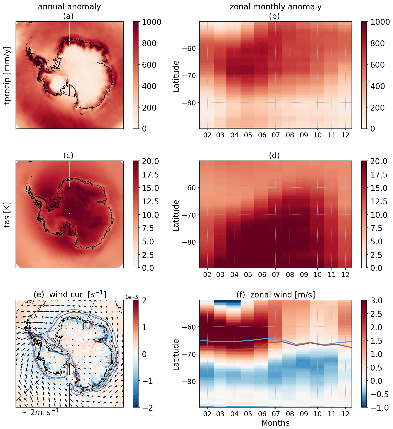
Figure 1Maps of annual mean anomalies (a, c, e) and monthly-mean zonal-mean anomalies (b, d, f) for (a, b) total precipitation and (c, d) near-surface air temperature, (e) near-surface wind curl and wind anomalies (arrows), and (f) near-surface zonal wind. In panels (e) and (f), the blue line is the position of the zero zonal wind in the JRA reanalysis, and the brown line is the equivalent for the perturbed wind.
Simulating realistic properties of the Southern Ocean and Antarctic marginal seas has often been challenging at a 0.25∘ resolution (e.g. Smith et al., 2021), largely because this resolution is in the grey zone between fully resolved and fully parameterised eddies. The present-day simulation described in this paper is the result of many months of empirical tuning, and it gives a relatively good representation of the ocean-ice properties in the Southern Ocean. We therefore provide an extensive evaluation of this simulation. The results presented here are based on the climatology of the last 10 years of the present-day simulation, i.e. the period spanning from 2009 to 2018.
3.1 General circulation
The Antarctic Circumpolar Current (ACC) barotropic transport across Drake Passage is 137 Sv (sverdrup) in REF. It compares reasonably well with estimates derived from observations and ocean model reanalyses. Equivalent observational estimates indeed reached 137 ± 8 Sv (Cunningham et al., 2003), 173 ± 11 Sv (Donohue et al., 2016), and 141 ± 13 Sv (Koenig et al., 2014). Ocean reanalyses give an average transport across Drake Passage of 153 ± 5 Sv in SOSE (Southern Ocean State Estimate; Mazloff et al., 2010), 155 Sv in GLORYS12 (Mercator global ocean reanalysis; Lellouche et al., 2021; Artana et al., 2021), and 152 ± 19 Sv in an ensemble long‐term mean transport from nine ocean reanalysis products (Uotila et al., 2019).
The barotropic transport within the Ross and Weddell gyres is reasonably well represented in REF, with 26 Sv and 60 Sv, respectively, as estimated from the maximum barotropic stream function in the southern limb of each gyre (Fig. 2). This is slightly stronger than the equivalent estimates in the SOSE reanalysis (20 ± 5 and 40 ± 8 Sv within the Ross and Weddell gyres in Mazloff et al., 2010). This is nonetheless closer to the observation-based barotropic transport for the Weddell Gyre: 56 ± 8 Sv across the prime meridian (Klatt et al., 2005) and 83 ± 22 Sv in the south-eastern limb of the gyre (Reeve et al., 2019).
The shape of these gyres is also realistic (Fig. 2). The Weddell Gyre in REF has a similar shape as the one derived from observations by Reeve et al. (2019, their Fig. 4), although our maximum is located along the prime meridian, i.e. ∼ 15∘ westward of their observational estimate. Characterising the gyre extent by the barotropic stream function at half of its maximum value within the gyre, the Weddell Gyre extends eastward to 45∘ E in REF vs. 30∘ E in SOSE. Similarly, the Ross Gyre sits within 180–220∘ E in REF vs. 160–220∘ E in SOSE (Mazloff et al., 2010).
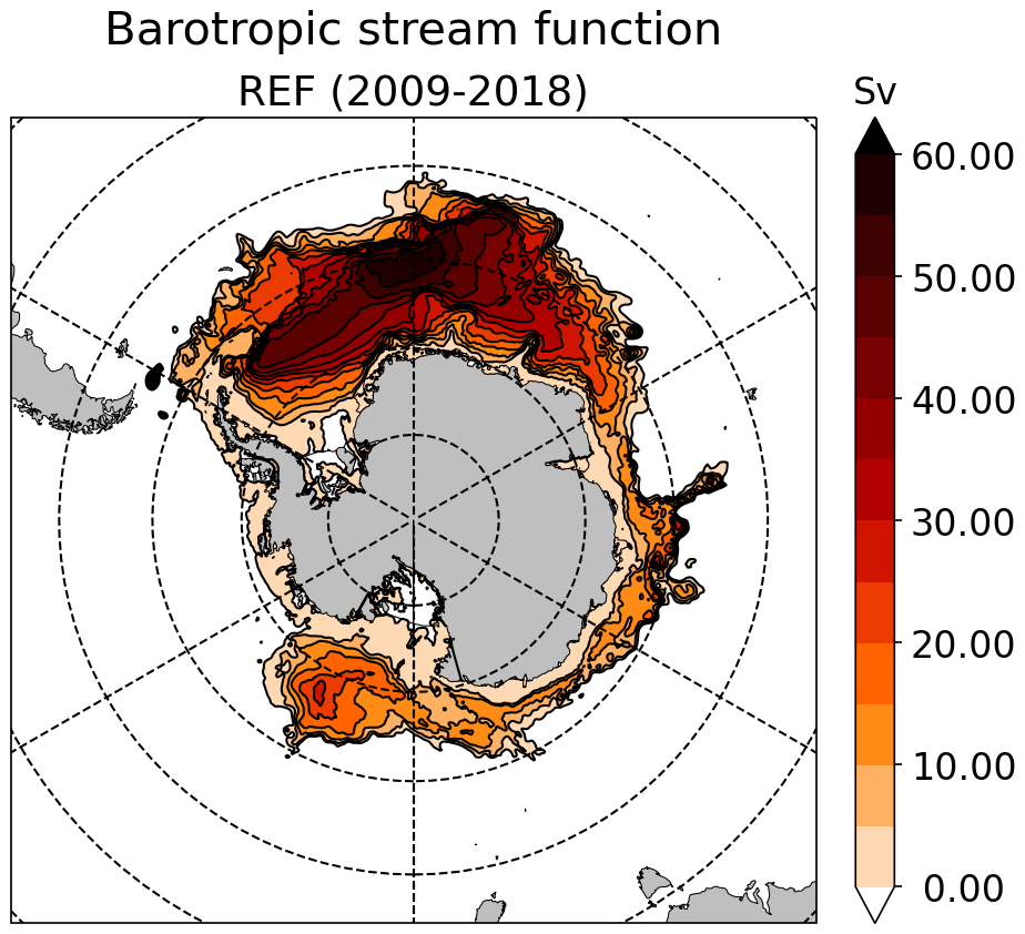
Figure 2Climatological (2009–2018) barotropic stream function (Ψ) in REF (contours every 10 Sv). Areas beyond the polar gyres are in white. The zonal and meridional barotropic transports (Sv) between two locations are given by and V=ΔxΨ, i.e. by the signed differences in Ψ between these two points.
3.2 Sea ice and water mass properties on the continental shelf
Our REF simulation captures very well the maximum sea ice extent (Fig. 3b), with a September average of 18.3×10⁶ km2 in REF vs. 18.7×10⁶ km2 in the satellite product of Meier et al. (2021). REF underestimates the minimum sea ice extent (Fig. 3a), with 2.5×10⁶ km2 on average in February vs. 3.1×10⁶ km2 in the satellite product of Meier et al. (2021). This underestimation is mostly due to the missing summer sea ice along the East Antarctic coast (Fig. 3a). A possible explanation for this is the absence of polynyas associated with thick sea ice fastened to grounded icebergs (Nihashi et al., 2017), which would require a specific parameterisation of the sea ice tensile stress (Van Achter et al., 2022), an iceberg grounding scheme, and two-way iceberg–sea-ice interactions in NEMO.
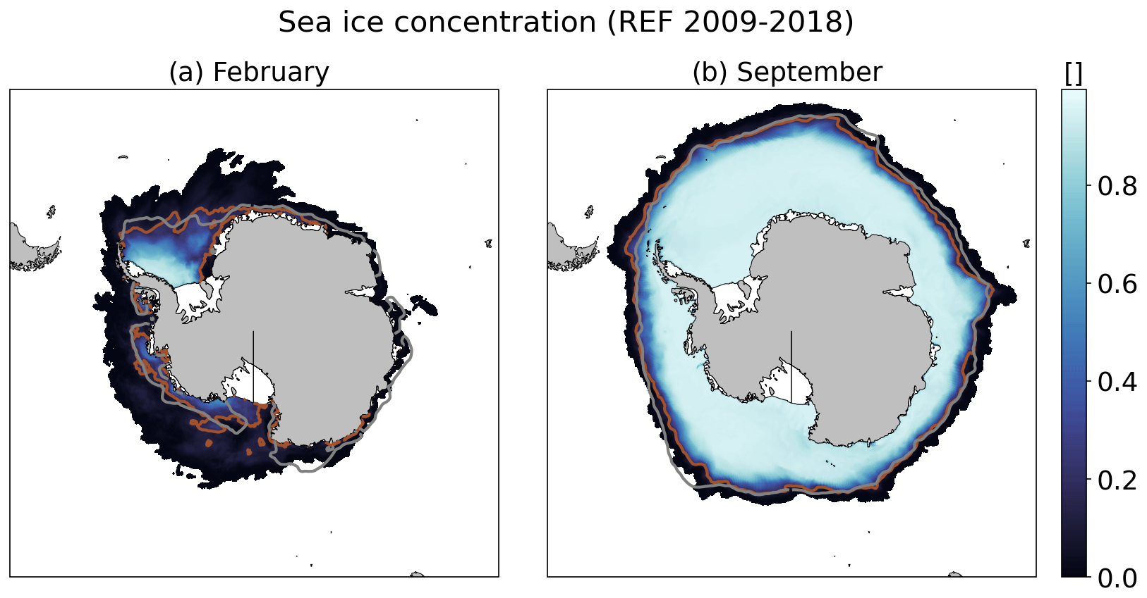
Figure 3Climatological (2009–2018) sea ice concentration in REF in (a) February and (b) September. The grey lines indicate the sea ice extent in the satellite product of Meier et al. (2021), and the brown line shows the equivalent in our REF simulation.
The presence of High Salinity Shelf Water (HSSW) is important both because it is a precursor for the Antarctic Bottom Water, which is key for the global thermohaline circulation, and because it controls the circulation in cold ice shelf cavities (e.g. Janout et al., 2021). Our REF simulation produces HSSW in the Ross Ice Shelf and Terra Nova Bay polynyas (western Ross Sea) and in the Ronne polynya (western Weddell Sea) with a reasonable fresh bias of ∼ 0.05 g kg−1 (Fig. 4a, b). REF is also slightly too fresh in Prydz Bay, near Amery Ice Shelf, another area known for HSSW production (Herraiz-Borreguero et al., 2015), and in East Antarctica in general, likely due to the aforementioned absence of iceberg-induced polynyas (Fig. 4c).
In terms of bottom temperatures, REF represents weakly modified Circumpolar Deep Water (CDW) in the Bellingshausen Sea and Amundsen Sea, in good agreement with WOA2018 data (Fig. 4c, d). This is an improvement compared to previous circum-Antarctic studies at similar resolution (e.g. Mathiot et al., 2017; Naughten et al., 2018b). As observed, the bottom Weddell and Ross seas and the adjacent ice shelf cavities are filled with water near the surface freezing point (−1.9 ∘C). The simulated bottom temperatures are colder than WOA2018 in the Indian Ocean sector of East Antarctica compared to WOA2018 with the exception of Prydz Bay/Amery Ice Shelf (Fig. 4f). This comparison should be considered with caution given the sparse observations in this region. Relatively warm water at depth was observed in the vicinity of Totten Ice Shelf and Vincennes Bay, but the presence of cold water was reported at other locations in this sector (Rintoul et al., 2016; Ribeiro et al., 2021; Portela et al., 2022). The north end of the Antarctic Peninsula also exhibits a cold bias in REF. Preliminary analyses during the tuning process suggested that this bias was sensitive to the HSSW properties (worse when HSSW was not dense enough), to the treatment of the bathymetry, and to the lateral slip condition and bottom friction at the tip of peninsula.
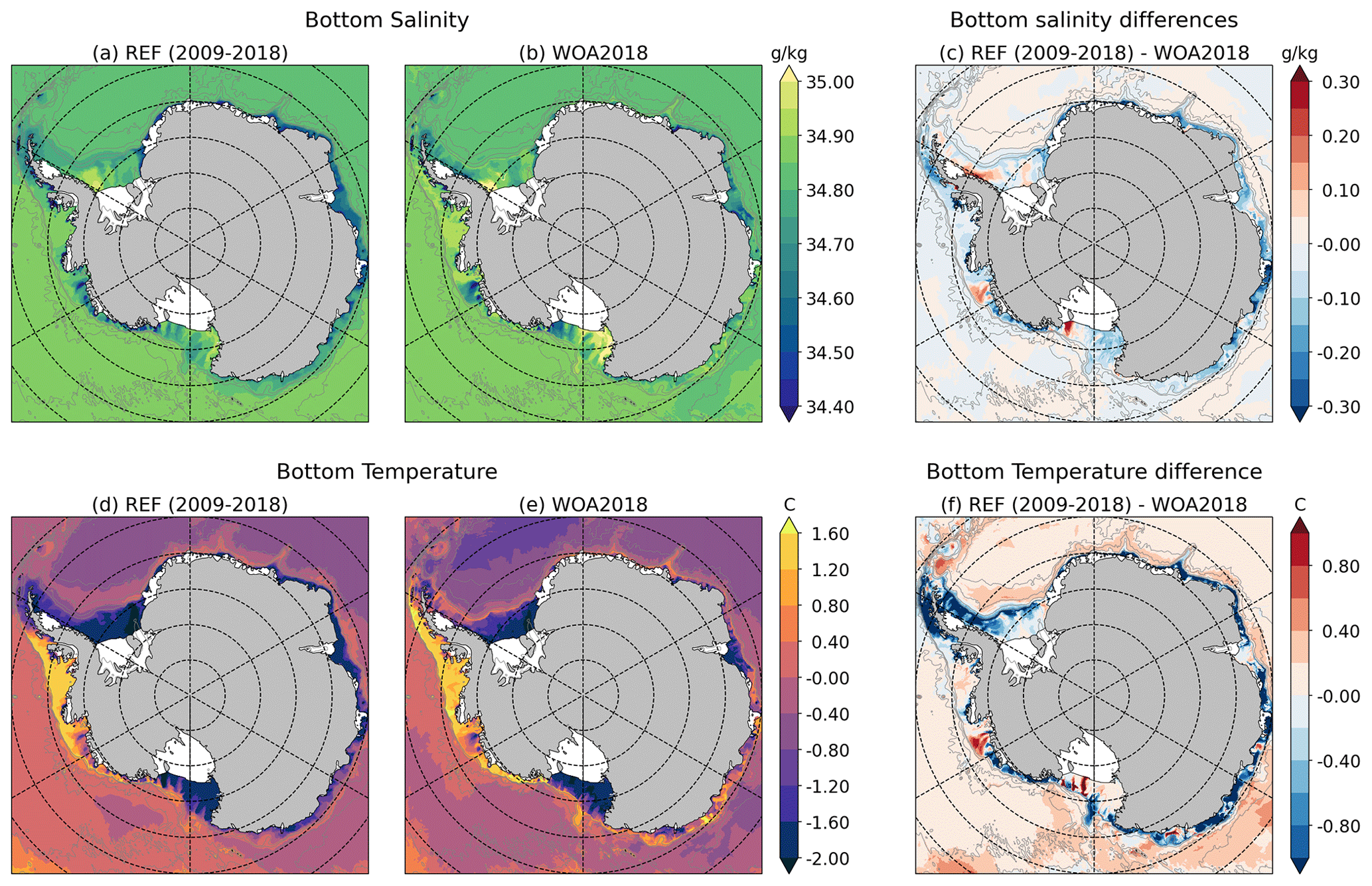
Figure 4(a, b, c) Climatological bottom practical salinity in (a) REF, (b) WOA2018 (Locarnini et al., 2019; Zweng et al., 2019), and (c) the difference REF-WOA2018. (d, e, f) Climatological conservative temperature in (d) REF, (e) WOA2018, and (f) the difference.
3.3 Ice shelf melt
Our ocean model configuration represents 1.48×10⁶ km2 of ice shelves, and their simulated rate of basal mass loss is 1182 Gt yr−1 (gigatonne per year) over 2009–2018, which compares well with the 1325±235 Gt yr−1 rate in the 2000s for a surveyed area of 1.55×10⁶ km2 in Rignot et al. (2013) and with the 965±265 Gt yr−1 rate over 1992–2017 for a surveyed area of 1.54×10⁶ km2 in Paolo et al. (2023).
The mean basal mass loss of individual ice shelves is generally in agreement with observational estimates (Fig. 5b). The melt rates are particularly overestimated for George VI Ice Shelf (a long-standing bias in NEMO), while they are significantly underestimated for the Thwaites Ice Shelf. For Thwaites, it should be noticed that we use a recent ice shelf draft in NEMO (Morlighem et al., 2020; Morlighem, 2020) with a significantly reduced area compared to the period covered by Rignot et al. (2013), which logically decreases the integrated melt. The total melt underneath Getz was strongly overestimated in preliminary simulations, reaching 400–500 Gt yr−1 (not shown). By reducing the ice shelf draft of Getz (Sect. 2), we have artificially displaced it into the model cold mixed layer, which gives more realistic melt rates. This empirical correction of the ice shelf draft is nonetheless slightly too strong because it was done prior to the completion of parameter tuning.
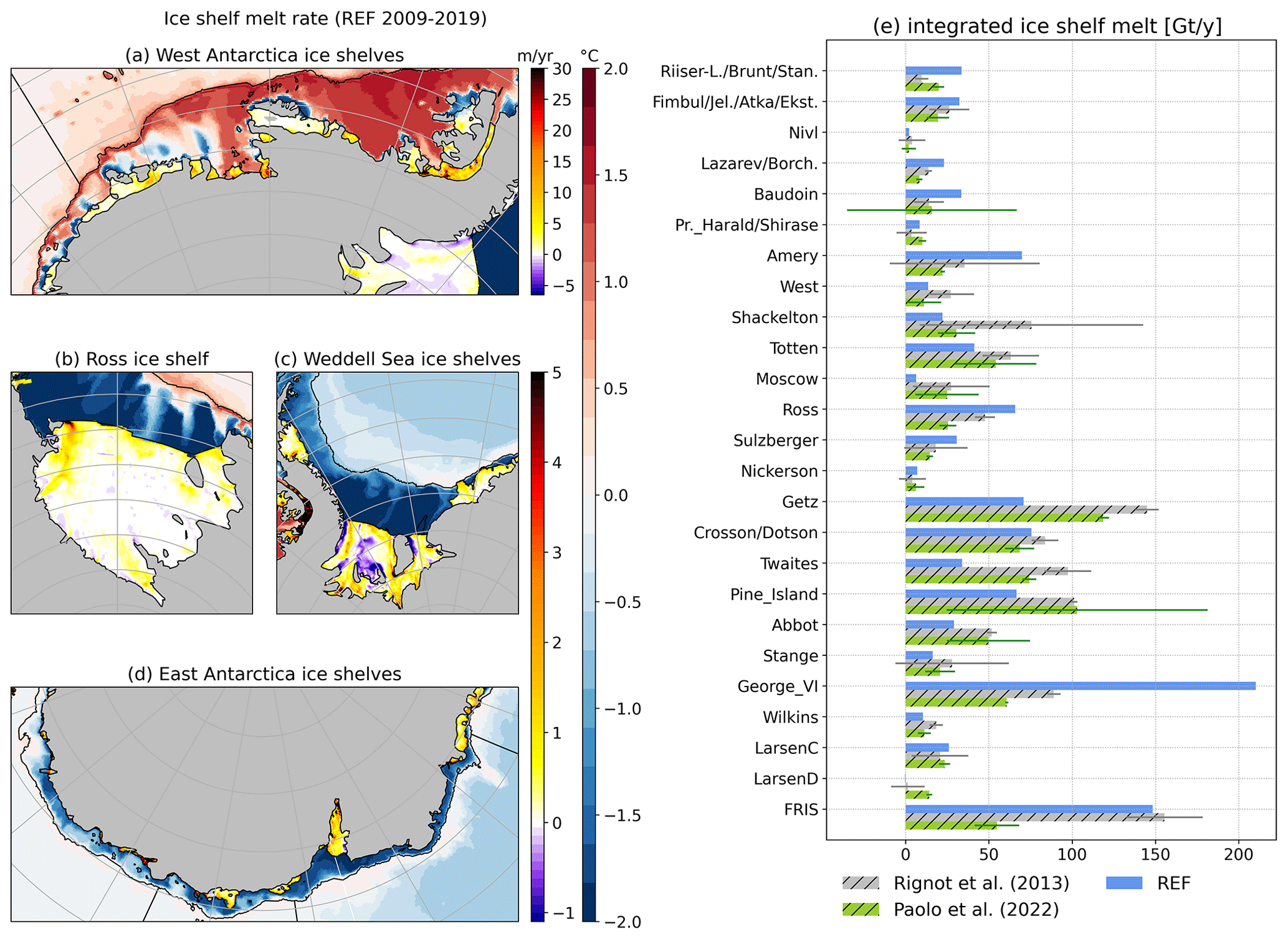
Figure 5(a–d) Climatological ice shelf melt rate per sector (purple to red colour map) with ocean bottom temperature on the Antarctic continental shelf (blue to red colour map) in REF (2009–2018). (e) Basal mass loss of individual ice shelves in REF (in Gt yr−1) averaged over the period 2009–2018. The observation-based estimates from Rignot et al. (2013) and Paolo et al. (2023) are respectively in black and gray. For clarity, the ice shelves smaller than 4000 km2 in Rignot et al. (2013) are not represented. See Fig. 1 in Rignot et al. (2013) for the locations of individual ice shelves.
The simulated ice shelf melt rate pattern is shown in Fig. 5a. The melt pattern underneath the Filchner-Ronne Ice Shelf includes large areas of refreezing and maximum melt rates at the front of Ronne Ice Shelf and near the deepest parts of the grounding line, consistent with satellite estimates (Rignot et al., 2013; Moholdt et al., 2014; Adusumilli et al., 2020) and high-resolution simulations (Hausmann et al., 2020). Near-zero melt rates are simulated underneath most of the Ross Ice Shelf, except near Ross Island at the west end of the ice front, as reported by Rignot et al. (2013) and Adusumilli et al. (2020). The warm ice shelves from Getz to Pine Island, in the Amundsen Sea, all experience local melt rates above 10 m yr−1 in agreement with the aforementioned satellite estimates. The deepest part of Pine Island shows a high melt area above 20 m yr−1, corresponding to the one visible in satellite data (Shean et al., 2019), although simulated melt rates there are underestimated by approximately a factor of 2. This underestimation near the grounding line may be due to a lack of horizontal and vertical resolution in this area (the melt pattern is more realistic at ; Jourdain et al., 2022) as well as the absence of subglacial runoff (Nakayama et al., 2021). Another noticeable bias is the absence of refreezing area beneath Amery Ice Shelf compared to satellite products (Wen et al., 2010; Rignot et al., 2013; Adusumilli et al., 2020), possibly related to the aforementioned lack of polynya activity upstream of Amery Ice Shelf.
3.4 Interannual variability in the Amundsen Sea
The vertical stratification and the interannual-to-decadal variability of ice shelf basal melt rates as well as ocean properties in front of the ice shelves are well documented for the Amundsen Sea thanks to recurrent oceanic cruises (e.g. Jacobs et al., 1996; Dutrieux et al., 2014; Jenkins et al., 2018). The simulated temperature profiles near Dotson Ice Shelf and Pine Island are overall within the interannual observational range, although the simulated thermocline is sharper and shallower than observed (Fig. 6e, f). Our REF simulation captures the transition to a relatively warm period between approximately 2005 and 2010, although the prior and posterior cold states remain significantly warmer than observed (Fig. 6c, d). As a consequence, the interannual variability of ice shelf melting is underestimated for both Dotson and Pine Island (Fig. 6a, b).
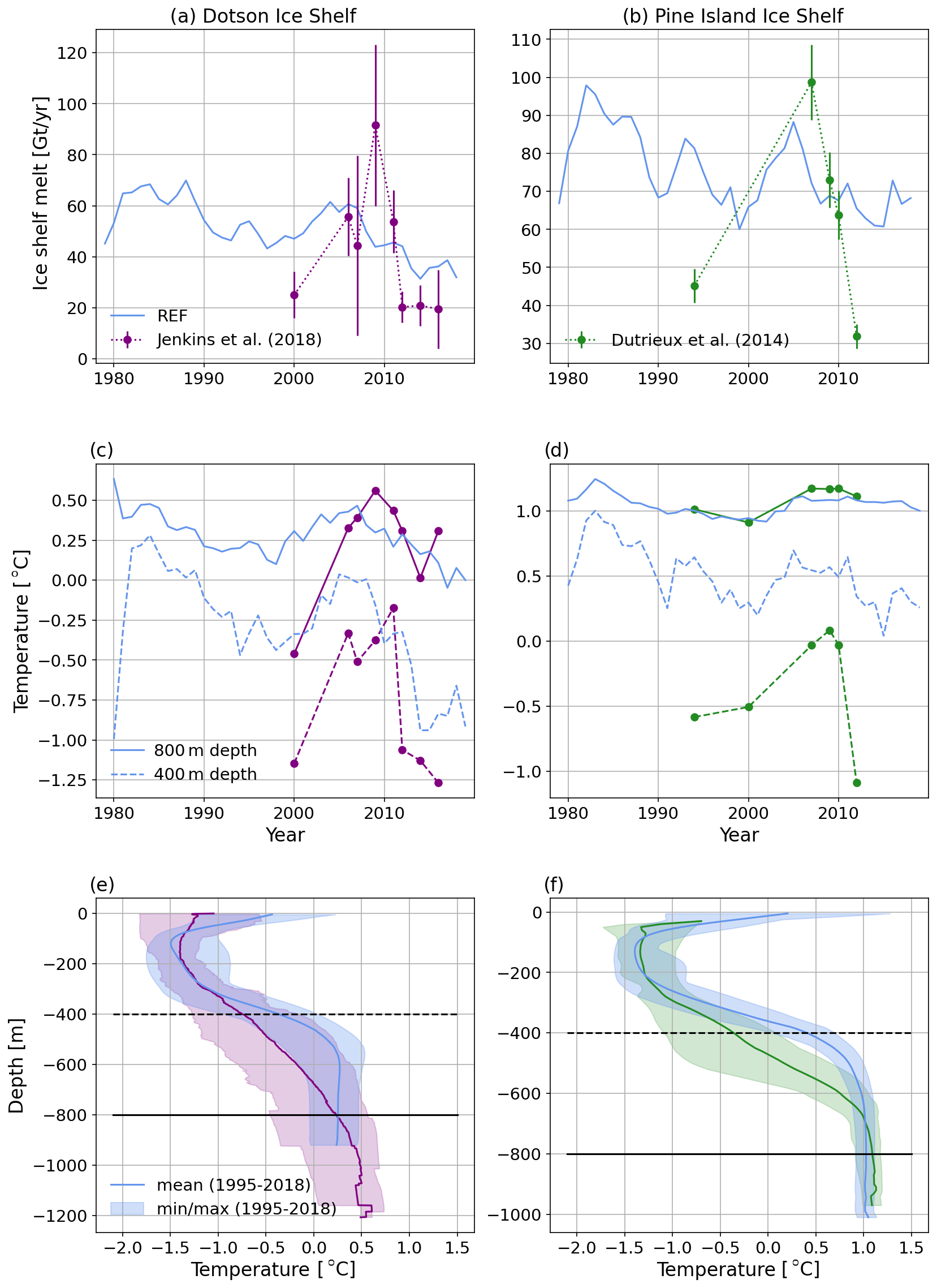
Figure 6Model evaluation of Dotson (a, c, e) and Pine Island (b, d, f) ice shelves. Simulated properties are in blue, while observational estimated are in red for Dotson (Jenkins et al., 2018) and in green for Pine Island (Dutrieux et al., 2014). (a, b) Melt time series, (c, d) potential temperature time series at 400 and 800 m depth in front of the ice shelves, and (e, f) mean December-to-February temperature profile between 1995 and 2018 and near the ice shelf front, as well as the minimum–maximum interannual range (shaded).
4.1 General circulation and sea ice
The ocean barotropic circulation undergoes a strong adjustment to the perturbation in the first 5 to 10 years, followed by a slower drift to nearly a steady state reached after approximately 80 years of perturbation (Fig. 7). The Weddell Gyre strengthens by ∼30 % (Fig. 7a) and extends further east, reaching Prydz Bay. The westward slope current constituting the southern flank of the gyre is highly intensified across the Weddell Sea (Fig. 8). The Ross Gyre is doubled in intensity (Fig. 7b) and extends further east, reaching the Bellingshausen Sea and Amundsen Sea (Fig. 8). This is consistent with changes in wind stress curl due to changes in the atmospheric circulation (Fig. 1e) and sea ice loss, as previously reported in projections over the 21st century (Gómez-Valdivia et al., 2023). The ACC transport decreases to 110–115 Sv (Fig. 7c), likely due to a shutdown of HSSW and Antarctic Bottom Water (AABW) formation as very little sea ice is produced in the perturbed experiment. There is indeed no sea ice left in summer, and the maximum sea ice area declines from 18×106 km2 to less than 1×10⁶ km2 in September (not shown).
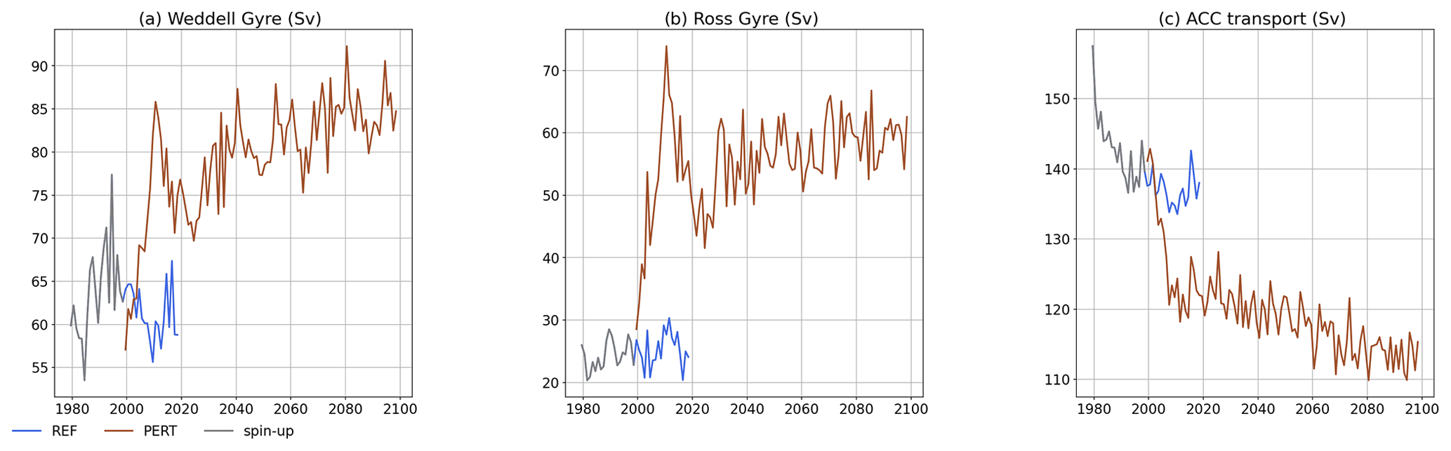
Figure 7Time series of the Weddell Gyre (a), Ross Gyre (b), and ACC transport (c) in REF (brown) and PERT (blue).
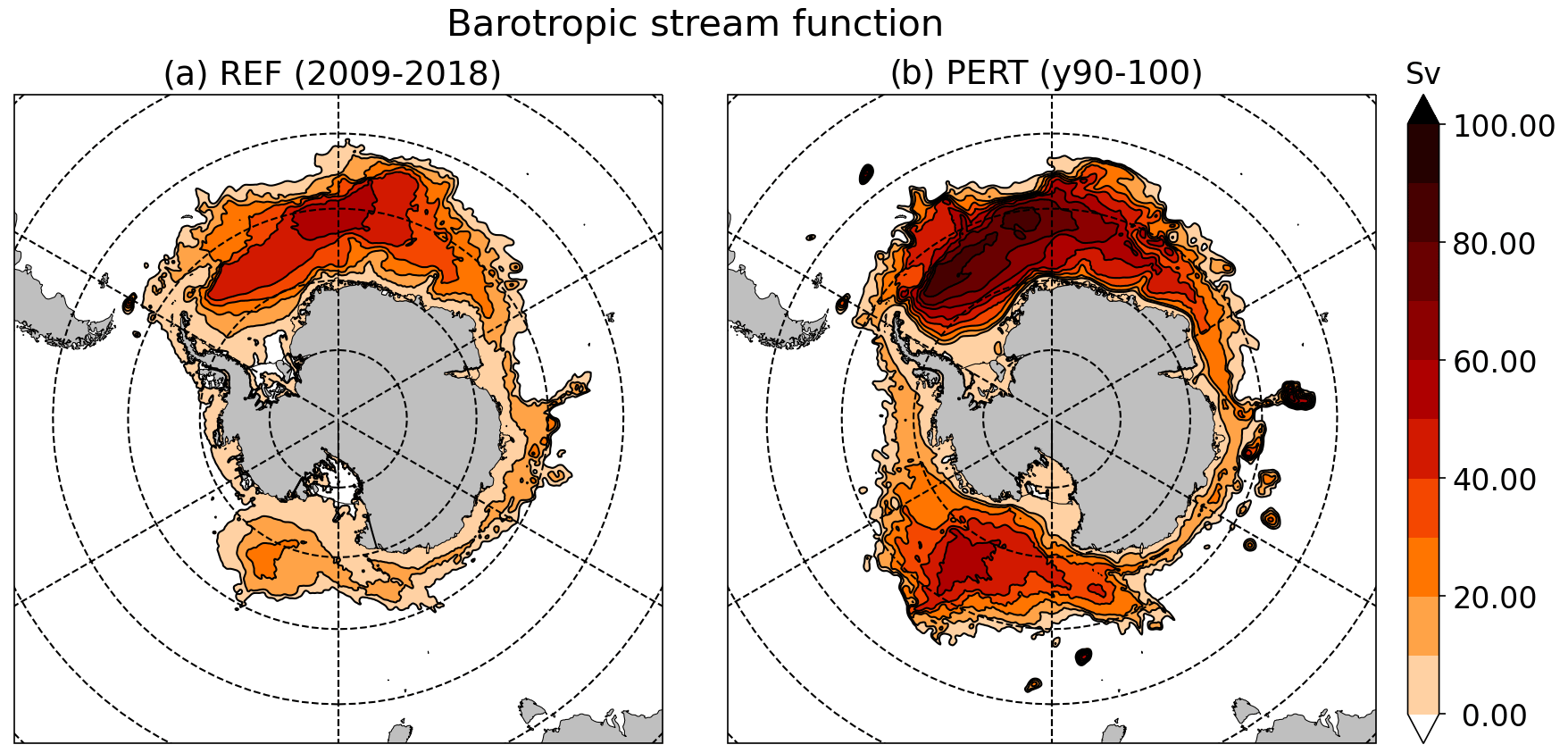
Figure 8Climatological barotropic stream function in REF (a) and PERT (b). In white is the area beyond the polar gyres. Each contour is 10 Sv.
4.2 Water mass properties on the continental shelf
The general picture is that sea ice production becomes insufficient to maintain HSSW on the continental shelf, which decreases the density barrier between cold shelf water and CDW, thereby enabling CDW flows onto the continental shelf (Naughten et al., 2021). This is particularly visible in the first 10 years of the perturbed simulations, at the Ronne depression (WWED box in Fig. 9b) and the Victoria Land Basin (WROSS box in Fig. 9d), two major sites of HSSW formation. CDW intrusions first occur on the eastern part of these seas, in the Filchner Trough (EWED box in Fig. 9a) and Little America Basin (EROSS box in Fig. 9c). The rapid initial adjustment to the new forcing is followed by a slow trend toward freshening and warming, which can be explained by slow changes in deep ocean properties at the circum-Antarctic scale (Sallée et al., 2013).
Figure 9Left: temperature vertical profile as a function of time in PERT, averaged in east Weddell box (a), east Ross box (c), and Amundsen Sea box (e). Right: salinity vertical profile as a function of time in PERT, averaged in west Weddell box (a), west Ross box, (b) and Amundsen Sea box (c). See inset in panel (b) for box definitions.
Figure 10(a–c) Temperature cross-section across the Amundsen Sea. (b–d) Temperature cross-section across the Dumont d'Urville Sea. The coloured contours are isopycnals, and the black contours show the zonal velocity every 5 cm s−1 (dashed/solid lines for westward/eastward velocity, gray line for zero velocity). (e–f) Sea surface height profile along the corresponding sections (blue for REF and brown for PERT).
The Amundsen Sea becomes warmer than present-day conditions within 20 years, with very slow increase afterwards (Fig. 9e). By the end of perturbation, bottom temperatures warm by 2 ∘C on the Amundsen Sea shelf. This is a much stronger warming than those obtained by Caillet et al. (2022) from local atmospheric perturbations typical of 2300, likely due to the expansion of the Ross Gyre in our simulations (Fig. 8), while Caillet et al. (2022) used constant far-field ocean circulation. In a warmer climate, the Ross Gyre is indeed projected to grow toward the Amundsen–Bellingshausen seas, which favours CDW intrusion onto the continental shelf, leading to a subsurface warming that may exceed 1 ∘C by 2100 on the continental shelf (Gómez-Valdivia et al., 2023).
To further illustrate the processes in place, we now compare a section across the Dumont d'Urville Sea (north of Adélie Land) with a section in the Eastern Amundsen Sea, which can presently be classified as “dense shelf” and “warm shelf”, respectively (Thompson et al., 2018). The former is characterised by cold and dense/salty water on the shelf and the second by the presence of weakly modified CDW at depth (Fig. 10). In the perturbed experiment, both locations are characterised by the presence of CDW (typical of a “warm shelf”) and very strong vertical and northward density gradients both typical of a “fresh shelf” (Thompson et al., 2018). We therefore suggest to classify this as “warm–fresh shelf”, in which the cold Antarctic Surface Water usually found over fresh shelves is replaced by a fresh and warm water mass overlaying a saltier CDW layer. The very strong density gradients in the perturbed experiments are a result of decreased sea ice production and subsequent convection, combined with increased ice shelf melting and precipitation, as well as icebergs melting closer to Antarctica.
Figure 11(a–d) Climatological ice shelf melt rate per sector (purple to red colour map) with bottom temperature on the Antarctic continental shelf (blue to red colour map) in PERT after 100 years of perturbation. (e) Total basal melt per ice shelf (in Gt yr−1) in PERT (blue) and REF (brown). For clarity, only ice shelves larger the 4000 km2 in Rignot et al. (2013) are represented. Numbers in panel (e) indicate the relative contribution of individual ice shelves with respect to the total Antarctic melt in REF (blue) and PERT (brown).
Figure 12(a, b) Barotropic stream function (in Sv; see caption of Fig. 2) under the Filchner-Ronne Ice Shelf in REF (a) and PERT (b). (c) Ocean temperature section along Filchner-Ronne Ice Shelf front in PERT (see thick black line on the map inset). Contours are the velocities normal to the section (positive toward the cavity and negative toward the open ocean).
In the perturbed scenario, the circumpolar zonal winds are shifted southward (Fig. 1e, f), which increases sea surface height over the continental shelf through southward Ekman transport (Fig. 10e, f), as previously reported by Spence et al. (2014) in future projections. In the Amundsen and Bellingshausen seas, changes in the Ekman transport are also linked to more cyclonic wind in a warmer climate (Fig. 1 and Gómez-Valdivia et al., 2023). By geostrophy, this wind perturbation induces a westward surface current above the shelf break (Fig. 10). The strong northward density gradient due to the shelf freshening have an opposite effect that accumulates with depth (“thermal wind” effect), which tends to cancel or revert eastward the current near the sea floor (Fig. 10). This weak or eastward zonal current near the sea floor at the shelf break favours the intrusion of CDW onto the shelf (e.g. Wåhlin et al., 2012; Walker et al., 2013).
Our results are quite different from Spence et al. (2014), who found a flattening of the isopycnals in response to poleward shifting winds. This is likely because they did not represent the changes in air temperature, precipitation and ice shelf melt. Our proposed mechanism is more similar to the baroclinic response proposed by Silvano et al. (2022), except that the increased density gradient is not only due to the accumulation of surface water on the shelf through Ekman transport, but also to the coastal freshening induced by decreased sea ice production, increased ice shelf melting and increased precipitation.
The only area of the continental shelf that remains cold after 100 years of perturbation is the Ronne depression (Fig. 11c), where a specific mechanism is at play. In the reference simulation, significant amounts of HSSW are formed in the Ronne depression and flow under the Ronne Ice Shelf (Fig. 12a). In the perturbed experiment, the Ronne depression is occupied by water flowing out of the Ronne cavity and coming all the way from the Filchner trough and Central Trough (Fig. 12b). Despite a strong inflow of warm water into the Filchner and central troughs, there is still refreezing underneath Ronne (see following subsection) and water colder than surface freezing point is produced and exported out of the cavity (Fig. 12c). This indicates that all the heat that comes into the Filchner-Ronne cavity is consumed to melt the ice shelf even in a much warmer climate. It should be noted that this presence of cold outflow was not found by Naughten et al. (2021) in their abrupt-4xCO2 experiments corresponding to a lower warming level than in our study.
4.3 Ice shelf melt rates
As expected, ice shelf basal melt rates follow the same trend as bottom temperatures on the nearby continental shelf in response to the forcing perturbation. The total Antarctic melt increases 11-fold from 1180 to 15 700 Gt yr−1. The Antarctica averaged melt rate increased from 0.80 to 10.64 m yr−1 (metre water equivalent).
All present-day cold cavities, such as Ross, Amery, and Filchner, become warm in the perturbed experiment, and melt rates reach levels similar to those currently observed in the Amundsen Sea (Fig. 11). The present-day warm cavities, in the Amundsen and Bellingshausen seas, also experience increased melt rates, which are explained both by the warming resulting from the eastward extension of the Ross Gyre (Fig. 8 and Gómez-Valdivia et al., 2023) and by the strong warming of the winter mixed layer (between 100 and 250 m depth in Fig. 9c), resulting from the strong reduction of sea ice production in winter. The melt increase is particularly strong for Abbot and Getz ice shelves (Fig. 11), because a large portion of the ice draft is currently located in the cold winter mixed layer (Cochran et al., 2014; Wei et al., 2020) and experiences a shift to much warmer conditions in the perturbed experiment. Given that the position of the thermocline with respect to the ice draft largely drives the transition to a high melting regime, we believe that the ice draft correction applied to Getz has made the transition more realistic.
The Ross and Pine Island ice shelves experience a sharp increase in basal melt rates in the first years of perturbation, followed by a stabilisation. As the Ross continental shelf changes from cold (near −2 ∘C) to warm (>2 ∘C) conditions, the relative change in thermal driving is very large and melt rates are multiplied by ∼ 30, reaching 2810 Gt yr−1 (Fig. 13). This is 3 times more than the 900 Gt yr−1 obtained by Siahaan et al. (2022) at the end of the 21st century under SSP5-8.5 with a Ross continental shelf at ∼ 2∘C. Despite this strong warming, the Ross ice shelf still exhibits a stable amount of refreezing (1 Gt yr−1) after the first decade (not shown).
As the Amundsen Sea is already warm in present-day conditions, the thermal driving at depth only doubles so that Pine Island and Thwaites experience a weaker relative increase in melt rates. For Crosson, Dotson, and Getz, the present-day ice shelf is partly located in the thermocline, so a part of these ice shelves experience larger relative increase in thermal driving. This results in an additional basal mass loss of ∼ 1000 Gt yr−1 due to the perturbation, which is much higher than the additional 350 Gt yr−1 obtained by Jourdain et al. (2022) for the entire Amundsen Sea sector at the end of the 21st century under SSP5-8.5.
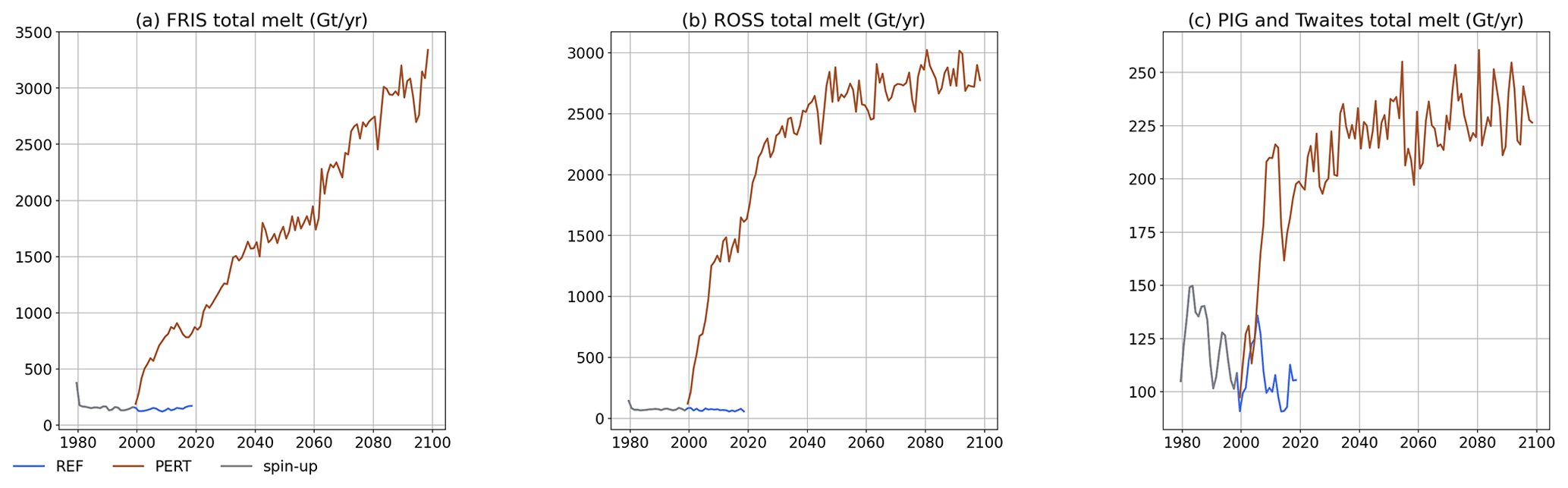
Figure 13Total ice shelf melt time series in PERT for the Filchner-Ronne Ice Shelf (a), Ross Ice Shelf (b), and Pine Island (PIG) and Thwaites ice shelves (c).
The Filchner-Ronne Ice Shelf exhibits a distinct behaviour: melt rates increase steadily during 100 years, but there is still a stable and significant amount of refreezing (26 Gt yr−1) in the last decades of our experiment (Fig. 11). After 100 years, the basal mass loss of Filchner-Ronne reaches 3000 Gt yr−1, i.e. ∼ 20 times larger than in REF. In comparison, Naughten et al. (2021) simulated a peak mass loss of 1600 Gt yr−1 for similar bottom temperatures in the Filchner Trough (∼ 2.4∘C), while Haid et al. (2022) obtained a peak at 1800 Gt yr−1 for ∼ 1.7∘C.
Two aspects may explain these different sensitivities. First, we simulate a strong increase in melt rates near the ice shelf front because of the disappearance of the cold surface layer in our simulations. In the two other studies, the surface layer is still cold, and the presence of an interactive ice sheet allows the ice shelf to thin and thereby to partly remain in this cold layer. Second, our parameterisation of tide-induced mixing in the three-equation system (Jourdain et al., 2019) may have a significant effect on the Ross and Filchner-Ronne melt rates. While this parameterisation has a weak effect on present-day conditions because all the available heat is consumed anyway (Hutchinson et al., 2023), the abundance of warm water in the future may enhance its role in the largest ice shelf cavities.
As all the shelves turned warm, the main contributors to the total ice shelf melt in PERT are mainly the one with the largest area. In REF, the West Antarctic Ice Sheet and Antarctic Peninsula sectors are responsible for 49 % of the total melt for only 15 % of the total Antarctic ice shelf area. In PERT, this contribution falls to 20 %. In contrast, the three giant cold ice shelves (Ross, Filchner-Ronne, and Amery) are responsible for 50 % of the total melt in PERT versus 23 % in REF, for 65 % of the total area (Fig. 11).
In this study, we have presented an new set-up for the global NEMO configuration at 0.25∘ resolution (eORCA025). Thanks to a preliminary tuning of the sea ice model parameters and of the lateral and bottom boundary conditions at the northern end of the Antarctic Peninsula, we simulate realistic water masses in the Southern Ocean and on the Antarctic continental shelf. This is important as the performance of previous versions of eORCA025 was not good enough to be used in ocean–ice-sheet simulations (Smith et al., 2021). The simulated basal mass loss of Antarctic ice shelves is 1180 Gt yr−1 on average, which aligns well with the observational estimates. Simulating the interannual variability in the Amundsen Sea nonetheless remains challenging, with an underestimated variability in our simulations.
We have then used this configuration to investigate the ocean and sea ice response to a strong and abrupt perturbation of the atmospheric conditions. To our knowledge, our study is the first to investigate plausible conditions for the late 23rd century at the scale of Antarctica under a high-end scenario (SSP5-8.5 and high equilibrium climate sensitivity of the driving climate model). Our simulations reveal that the entire Antarctic continental shelf is subject to substantial warming within the first 2 decades of perturbation and several decades of adjustment for the largest ice shelf cavities. In particular, the Filchner-Ronne Ice Shelf has a response time exceeding 100 years.
Our perturbation experiment is idealised in many ways. The abrupt transition to late 23rd century conditions does not account for slow changes in the global thermohaline circulation, including the formation of CDW very far from the Southern Ocean. At these timescales, interactions with the evolving ice sheet and atmosphere should also be taken into account for more realistic simulations (e.g. Donat-Magnin et al., 2017; Bronselaer et al., 2018; Bell et al., 2018). In this sense, future model intercomparisons with more realistic perturbations under strong emission scenarios will be needed. We nonetheless believe that we have identified key mechanisms that set the primary characteristics of the ocean and ice shelf response to strong climate perturbations, as described hereafter.
Under warmer atmospheric conditions, the sea ice cover drastically diminishes, even during winter, and the production of HSSW ceases, resulting in a rapid freshening of the previously salty continental shelves. In the absence of HSSW production, the intrusion of CDW onto the former cold continental shelves (Ross, Weddell, and East Antarctica) becomes more pronounced, although the rate of change may vary in different locations. These alterations in oceanic properties lead to a substantial increase in ice shelf melt rates, with a total basal mass loss escalating from 1180 to 15 700 Gt yr−1 after 100 years of perturbation. This significant increase is primarily attributed to the former colder ice shelves, which experience a substantial enhancement in thermal driving as they transition from cold cavities to warm cavities. In contrast, the relative change in ice melt rate for the warm cavities is comparatively smaller than that of the cold cavities.
Source code and parameter namelists for each experiment, as well as script used to make the figures, are all available here (https://github.com/pmathiot/paper_MJ2023) or here (https://doi.org/10.5281/zenodo.8411091, Mathiot, 2023).
Data used to run the simulations are available upon request to the lead author. Monthly atmospheric forcing anomalies as well as monthly climatologies of the last 30 years of PERT and REF are available on Zenodo (Mathiot and Jourdain, 2023).
PM conducted the numerical experiments, analysed and visualised the results, and led the writing process; NCJ contributed to the experimental design, to the results analysis, and to the writing process.
The contact author has declared that neither of the authors has any competing interests.
Publisher’s note: Copernicus Publications remains neutral with regard to jurisdictional claims made in the text, published maps, institutional affiliations, or any other geographical representation in this paper. While Copernicus Publications makes every effort to include appropriate place names, the final responsibility lies with the authors.
This study was funded by the European Union's Horizon 2020 research and innovation programme under grant agreement no. 820575 (TiPACCs) and by the French National Research Agency under grant no. ANR-19-CE01-0015 (EIS). N. Jourdain was also supported by EU-H2020 grant nos. 101003536 (ESM2025) and 869304 (PROTECT). This work was granted access to the high-performance computing (HPC) resources of CINES and TGCC under allocations A0100106035 and A0120106035 attributed by GENCI.
This research has been supported by the Horizon 2020 (grant nos. 820575, 101003536, and 869304) and the French National Research Agency (EIS (grant no. ANR-19-CE01-0015)), and the EU-H2020 (ESM2025 (grant no. 101003536) and PROTECT (grant no. 869304)).
This paper was edited by Karen J. Heywood and reviewed by Kaitlin Naughten and one anonymous referee.
Adcroft, A. and Campin, J. M.: Rescaled height coordinates for accurate representation of free-surface flows in ocean circulation models, Ocean Model., 7, 269–284, https://doi.org/10.1016/j.ocemod.2003.09.003, 2004. a
Adusumilli, S., Fricker, H. A., Medley, B., Padman, L., and Siegfried, M. R.: Interannual variations in meltwater input to the Southern Ocean from Antarctic ice shelves, Nat. Geosci., 13, 616–620, 2020. a, b, c
Agosta, C., Fettweis, X., and Datta, R.: Evaluation of the CMIP5 models in the aim of regional modelling of the Antarctic surface mass balance, The Cryosphere, 9, 2311–2321, https://doi.org/10.5194/tc-9-2311-2015, 2015. a
Agosta, C., Amory, C., Kittel, C., Orsi, A., Favier, V., Gallée, H., van den Broeke, M. R., Lenaerts, J. T. M., van Wessem, J. M., van de Berg, W. J., and Fettweis, X.: Estimation of the Antarctic surface mass balance using the regional climate model MAR (1979–2015) and identification of dominant processes, The Cryosphere, 13, 281–296, https://doi.org/10.5194/tc-13-281-2019, 2019. a
Artana, C., Ferrari, R., Bricaud, C., Lellouche, J.-M., Garric, G., Sennéchael, N., Lee, J.-H., Park, Y.-H., and Provost, C.: Twenty-five years of Mercator ocean reanalysis GLORYS12 at Drake Passage: Velocity assessment and total volume transport, Adv. Space Res., 68, 447–466, 2021. a
Asay-Davis, X. S., Cornford, S. L., Durand, G., Galton-Fenzi, B. K., Gladstone, R. M., Gudmundsson, G. H., Hattermann, T., Holland, D. M., Holland, D., Holland, P. R., Martin, D. F., Mathiot, P., Pattyn, F., and Seroussi, H.: Experimental design for three interrelated marine ice sheet and ocean model intercomparison projects: MISMIP v. 3 (MISMIP +), ISOMIP v. 2 (ISOMIP +) and MISOMIP v. 1 (MISOMIP1), Geosci. Model Dev., 9, 2471–2497, https://doi.org/10.5194/gmd-9-2471-2016, 2016. a
Barnier, B., Madec, G., Penduff, T., Molines, J.-M., Treguier, A.-M., Le Sommer, J., Beckmann, A., Biastoch, A., Böning, C., Dengg, J., Derval, C., Durand, E., Gulev, S., Remy, E., Talandier, C., Theetten, S., Maltrud, M., McClean, J., and de Cuevas, B.: Impact of partial steps and momentum advection schemes in a global ocean circulation model at eddy-permitting resolution, Ocean Dynam., 56, 543–567, 2006. a
Barthel, A., Agosta, C., Little, C. M., Hatterman, T., Jourdain, N. C., Goelzer, H., Nowicki, S., Seroussi, H., Straneo, F., and Bracegirdle, T. J.: CMIP5 model selection for ISMIP6 ice sheet model forcing: Greenland and Antarctica, The Cryosphere, 14, 855–879, https://doi.org/10.5194/tc-14-855-2020, 2020. a, b
Bell, R. E., Banwell, A. F., Trusel, L. D., and Kingslake, J.: Antarctic surface hydrology and impacts on ice-sheet mass balance, Nat. Clim. Change, 8, 1044–1052, 2018. a
Bett, D. T., Holland, P. R., Naveira Garabato, A. C., Jenkins, A., Dutrieux, P., Kimura, S., and Fleming, A.: The impact of the Amundsen Sea freshwater balance on ocean melting of the West Antarctic Ice Sheet, J. Geophys. Res.-Ocean., 125, e2020JC016305, https://doi.org/10.1029/2020JC016305, 2020. a
Boucher, O., Servonnat, J., Albright, A. L., et al.: Presentation and evaluation of the IPSL-CM6A-LR climate model, J. Adv. Model. Ea. Sys., 12, e2019MS002010, https://doi.org/10.1029/2019MS002010, 2020. a, b, c, d
Bouillon, S., Fichefet, T., Legat, V., and Madec, G.: The elastic–viscous–plastic method revisited, Ocean Model., 71, 2–12, https://doi.org/10.1016/j.ocemod.2013.05.013, 2013. a
Bronselaer, B., Winton, M., Griffies, S. M., Hurlin, W. J., Rodgers, K. B., Sergienko, O. V., Stouffer, R. J., and Russell, J. L.: Change in future climate due to Antarctic meltwater, Nature, 564, 53–58, https://doi.org/10.1038/s41586-018-0712-z, 2018. a, b
Bull, C. Y. S., Jenkins, A., Jourdain, N. C., Vaňková, I., Holland, P. R., Mathiot, P., Hausmann, U., and Sallée, J.-B.: Remote control of Filchner-Ronne ice shelf melt rates by the Antarctic slope current, J. Geophys. Res.-Ocean., 126, e2020JC016550, https://doi.org/10.1029/2020JC016550, 2021. a
Burgard, C., Jourdain, N. C., Reese, R., Jenkins, A., and Mathiot, P.: An assessment of basal melt parameterisations for Antarctic ice shelves, The Cryosphere, 16, 4931–4975, https://doi.org/10.5194/tc-16-4931-2022, 2022. a, b
Caillet, J., Jourdain, N. C., and Mathiot, P.: Abrupt cold-to-warm and warm-to-cold ocean transitions in the Amundsen Sea, Antarctica, J. Geophys. Res.-Ocean., 128, e2022JC018929, https://doi.org/10.1029/2022JC018929, 2022. a, b
Cochran, J. R., Jacobs, S. S., Tinto, K. J., and Bell, R. E.: Bathymetric and oceanic controls on Abbot Ice Shelf thickness and stability, The Cryosphere, 8, 877–889, https://doi.org/10.5194/tc-8-877-2014, 2014. a
Comeau, D., Asay-Davis, X. S., Begeman, C. B., Hoffman, M. J., Lin, W., Petersen, M. R., Price, S. F., Roberts, A. F., Van Roekel, L. P., Veneziani, M., Wolfe, J. D., Fyke, J. G., Ringler, T. D., and Turner, A. K.: The DOE E3SM v1. 2 Cryosphere Configuration: Description and Simulated Antarctic Ice-Shelf Basal Melting, J. Adv. Model. Ea. Sys., 14, e2021MS002468, https://doi.org/10.1029/2021MS002468, 2022. a
Cornford, S. L., Martin, D. F., Payne, A. J., Ng, E. G., Le Brocq, A. M., Gladstone, R. M., Edwards, T. L., Shannon, S. R., Agosta, C., van den Broeke, M. R., Hellmer, H. H., Krinner, G., Ligtenberg, S. R. M., Timmermann, R., and Vaughan, D. G.: Century-scale simulations of the response of the West Antarctic Ice Sheet to a warming climate, The Cryosphere, 9, 1579–1600, https://doi.org/10.5194/tc-9-1579-2015, 2015. a
Cunningham, S. A., Alderson, S. G., King, B. A., and Brandon, M. A.: Transport and variability of the Antarctic circumpolar current in drake passage, J. Geophys. Res.-Ocean., 108, C5, https://doi.org/10.1029/2001JC001147, 2003. a
Dai, A. and Trenberth, K. E.: Estimates of Freshwater Discharge from Continents: Latitudinal and Seasonal Variations, J. Hydrometeorol., 3, 660–687, https://doi.org/10.1175/1525-7541(2002)003<0660:EOFDFC>2.0.CO;2, 2002. a
DeConto, R. M., Pollard, D., Alley, R. B., Velicogna, I., Gasson, E., Gomez, N., Sadai, S., Condron, A., Gilford, D. M., Ashe, E. L., Li, D., and Dutton, A.: The Paris Climate Agreement and future sea-level rise from Antarctica, Nature, 593, 83–89, 2021. a
de Lavergne, C., Madec, G., Le Sommer, J., Nurser, A. J. G., and Naveira Garabato, A. C.: The Impact of a Variable Mixing Efficiency on the Abyssal Overturning, J. Phys. Oceanogr., 46, 663–681, https://doi.org/10.1175/JPO-D-14-0259.1, 2016. a
Donat-Magnin, M., Jourdain, N. C., Spence, P., Le Sommer, J., Gallée, H., and Durand, G.: Ice-Shelf Melt Response to Changing Winds and Glacier Dynamics in the Amundsen Sea Sector, Antarctica, J. Geophys. Res., 122, 10206–10224, 2017. a, b
Donat-Magnin, M., Jourdain, N. C., Kittel, C., Agosta, C., Amory, C., Gallée, H., Krinner, G., and Chekki, M.: Future surface mass balance and surface melt in the Amundsen sector of the West Antarctic Ice Sheet, The Cryosphere, 15, 571–593, https://doi.org/10.5194/tc-15-571-2021, 2021. a
Donohue, K. A., Tracey, K. L., Watts, D. R., Chidichimo, M. P., and Chereskin, T. K.: Mean antarctic circumpolar current transport measured in drake passage, Geophys. Res. Lett., 43, 11–760, 2016. a
Dutrieux, P., De Rydt, J., Jenkins, A., Holland, P. R., Ha, H. K., Lee, S. H., Steig, E. J., Ding, Q., Abrahamsen, E. P., and Schröder, M.: Strong sensitivity of Pine Island ice-shelf melting to climatic variability, Science, 343, 174–178, 2014. a, b
Forster, P., Storelvmo, T., Armour, K., Collins, W., Dufresne, J.-L., Frame, D., Lunt, D., Mauritsen, T., Palmer, M., Watanabe, M., and Zhang, H.: The Earth’s energy budget, climate feedbacks, and climate sensitivity, in: Climate Change 2021: The Physical Science Basis, Contribution of Working Group I to the Sixth Assessment Report of the Intergovernmental Panel on Climate Change, 923–1054, edited by: Masson-Delmotte, V., Zhai, P., Pirani, A., Connors, S. L., Péan, C., Berger, S., Caud, N., Chen, Y., Goldfarb, L., Gomis, M. I., Huang, M., Leitzell, K., Lonnoy, E., Matthews, J. B. R., Maycock, T. K., Waterfield, T., Yelekçi, O., Yu, R., and Zhou, B., Cambridge University Press, Cambridge, United Kingdom and New York, NY, USA, 923–1054, https://doi.org/10.1017/9781009157896.009, 2021. a
Gent, P. R. and Mcwilliams, J. C.: Isopycnal Mixing in Ocean Circulation Models, J. Phys. Oceanogr., 20, 150–155, https://doi.org/10.1175/1520-0485(1990)020<0150:IMIOCM>2.0.CO;2, 1990. a
Gladstone, R. M., Bigg, G. R., and Nicholls, K. W.: Iceberg trajectory modeling and meltwater injection in the Southern Ocean, J. Geophys. Res., 106, 19903–19915, 2001. a
Gómez-Valdivia, F., Holland, P. R., Siahaan, A., Dutrieux, P., and Young, E.: Projected West Antarctic ocean warming caused by an expansion of the Ross Gyre, Geophys. Res. Lett., 50, e2023GL102978, https://doi.org/10.1029/2023GL102978, 2023. a, b, c, d
Griffies, S. M., Biastoch, A., Böning, C., Bryan, F., Danabasoglu, G., Chassignet, E. P., England, M. H., Gerdes, R., Haak, H., Hallberg, R. W., Hazeleger, W., Jungclaus, J., Large, W. G., Madec, G., Pirani, A., Samuels, B. L., Scheinert, M., Sen Gupta, A., Severijns, C. A., Simmons, H. L., Treguier, A. M., Winton, M., Yeager, S., and Yin, J.: Coordinated ocean-ice reference experiments (COREs), Ocean Modell., 26, 1–46, 2009. a
Griffies, S. M., Danabasoglu, G., Durack, P. J., Adcroft, A. J., Balaji, V., Böning, C. W., Chassignet, E. P., Curchitser, E., Deshayes, J., Drange, H., Fox-Kemper, B., Gleckler, P. J., Gregory, J. M., Haak, H., Hallberg, R. W., Heimbach, P., Hewitt, H. T., Holland, D. M., Ilyina, T., Jungclaus, J. H., Komuro, Y., Krasting, J. P., Large, W. G., Marsland, S. J., Masina, S., McDougall, T. J., Nurser, A. J. G., Orr, J. C., Pirani, A., Qiao, F., Stouffer, R. J., Taylor, K. E., Treguier, A. M., Tsujino, H., Uotila, P., Valdivieso, M., Wang, Q., Winton, M., and Yeager, S. G.: OMIP contribution to CMIP6: experimental and diagnostic protocol for the physical component of the Ocean Model Intercomparison Project, Geosci. Model Dev., 9, 3231–3296, https://doi.org/10.5194/gmd-9-3231-2016, 2016. a
Haid, V., Timmermann, R., Gürses, Ö., and Hellmer, H. H.: On the drivers of regime shifts in the Antarctic marginal seas, EGUsphere [preprint], https://doi.org/10.5194/egusphere-2022-1044, 2022. a
Hausfather, Z. and Peters, G. P.: Emissions–the ‘business as usual’story is misleading, Nature, 577, 618–620, 2020. a
Hausmann, U., Sallée, J.-B., Jourdain, N. C., Mathiot, P., Rousset, C., Madec, G., Deshayes, J., and Hattermann, T.: The Role of Tides in Ocean-Ice Shelf Interactions in the Southwestern Weddell Sea, J. Geophys. Res.-Ocean., 125, e2019JC015847, https://doi.org/10.1029/2019JC015847, 2020. a, b
Herraiz-Borreguero, L., Coleman, R., Allison, I., Rintoul, S. R., Craven, M., and Williams, G. D.: Circulation of modified C ircumpolar D eep W ater and basal melt beneath the A mery I ce S helf, E ast A ntarctica, J. Geophys. Res.-Ocean., 120, 3098–3112, 2015. a
Heuzé, C.: Antarctic Bottom Water and North Atlantic Deep Water in CMIP6 models, Ocean Sci., 17, 59–90, https://doi.org/10.5194/os-17-59-2021, 2021. a
Holland, D. M. and Jenkins, A.: Modeling thermodynamic ice-ocean interactions at the base of an ice shelf, J. Phys. Oceanogr., 29, 1787–1800, 1999. a
Hutchinson, K., Deshayes, J., Éthé, C., Rousset, C., de Lavergne, C., Vancoppenolle, M., Jourdain, N. C., and Mathiot, P.: Improving Antarctic Bottom Water precursors in NEMO for climate applications, Geosci. Model Dev., 16, 3629–3650, https://doi.org/10.5194/gmd-16-3629-2023, 2023. a, b
Jacobs, S. S., Hellmer, H. H., and Jenkins, A.: Antarctic ice sheet melting in the Southeast Pacific, Geophys. Res. Lett., 23, 957–960, 1996. a
Janout, M. A., Hellmer, H. H., Hattermann, T., Huhn, O., Sültenfuss, J., Østerhus, S., Stulic, L., Ryan, S., Schröder, M., and Kanzow, T.: FRIS revisited in 2018: On the circulation and water masses at the Filchner and Ronne ice shelves in the southern Weddell Sea, J. Geophys. Res.-Ocean., 126, e2021JC017269, https://doi.org/10.1029/2021JC017269, 2021. a
Jenkins, A., Hellmer, H. H., and Holland, D. M.: The role of meltwater advection in the formulation of conservative boundary conditions at an ice-ocean interface, J. Phys. Oceanogr., 31, 285–296, 2001. a
Jenkins, A., Nicholls, K. W., and Corr, H. F. J.: Observation and parameterization of ablation at the base of Ronne Ice Shelf, Antarctica, J. Phys. Oceanogr., 40, 2298–2312, 2010. a
Jenkins, A., Shoosmith, D., Dutrieux, P., Jacobs, S., Kim, T. W., Lee, S. H., Ha, H. K., and Stammerjohn, S.: West Antarctic Ice Sheet retreat in the Amundsen Sea driven by decadal oceanic variability, Nat. Geosci., 11, 733–738, 2018. a, b
Jourdain, N. C., Mathiot, P., Merino, N., Durand, G., Le Sommer, J., Spence, P., Dutrieux, P., and Madec, G.: Ocean circulation and sea-ice thinning induced by melting ice shelves in the Amundsen Sea, J. Geophys. Res.-Ocean., 122, 2550–2573, 2017. a
Jourdain, N. C., Molines, J.-M., Le Sommer, J., Mathiot, P., Chanut, J., de Lavergne, C., and Madec, G.: Simulating or prescribing the influence of tides on the Amundsen Sea ice shelves, Ocean Model., 133, 44–55, 2019. a, b
Jourdain, N. C., Mathiot, P., Burgard, C., Caillet, J., and Kittel, C.: Ice Shelf Basal Melt Rates in the Amundsen Sea at the End of the 21st Century, Geophys. Res. Lett., 49, e2022GL100629, https://doi.org/10.1029/2022GL100629, 2022. a, b, c, d
Kittel, C., Amory, C., Agosta, C., Jourdain, N. C., Hofer, S., Delhasse, A., Doutreloup, S., Huot, P.-V., Lang, C., Fichefet, T., and Fettweis, X.: Diverging future surface mass balance between the Antarctic ice shelves and grounded ice sheet, The Cryosphere, 15, 1215–1236, https://doi.org/10.5194/tc-15-1215-2021, 2021. a
Klatt, O., Fahrbach, E., Hoppema, M., and Rohardt, G.: The transport of the Weddell Gyre across the Prime Meridian, Deep-Sea Res. Pt. II, 52, 513–528, 2005. a
Koenig, Z., Provost, C., Ferrari, R., Sennéchael, N., and Rio, M.-H.: Volume transport of the A ntarctic C ircumpolar C urrent: Production and validation of a 20 year long time series obtained from in situ and satellite observations, J. Geophys. Res.-Ocean., 119, 5407–5433, 2014. a
Krinner, G. and Flanner, M. G.: Striking stationarity of large-scale climate model bias patterns under strong climate change, P. Natl. Acad. Sci. USA, 115, 9462–9466, 2018. a, b
Krinner, G., Kharin, V., Roehrig, R., Scinocca, J., and Codron, F.: Historically-based run-time bias corrections substantially improve model projections of 100 years of future climate change, Comm. Ea. Env., 1, 1–7, 2020. a
Large, W. G. and Yeager, S. G.: Diurnal to decadal global forcing for ocean and sea-ice models: the data sets and flux climatologies, Tech. Rep. NCAR/TN-460+STR, National Center for Atmospheric Research, Boulder, Colorado, https://doi.org/10.5065/D6KK98Q6, 2004. a
Lee, J.-Y., Dunne, J. P., Engelbrecht, F., Fischer, E., Fyfe, J. C., Jones, C., A., M., Mutemi, J., Ndiaye, O., Panickal, S., and Zhou, T.: Future global climate: scenario-based projections and near-term information, Chap. 4, in: Climate Change 2021: The Physical Science Basis, Contribution of Working Group I to the Sixth Assessment Report of the Intergovernmental Panel on Climate Change, 553–672, edited by: Masson-Delmotte, V., Zhai, P., Pirani, A., Connors, S. L., Péan, C., Berger, S., Caud, N., Chen, Y., Goldfarb, L., Gomis, M. I., Huang, M., Leitzell, K., Lonnoy, E., Matthews, J. B. R., Maycock, T. K., Waterfield, T., Yelekçi, O., Yu, R., and Zhou, B., Cambridge University Press, Cambridge, United Kingdom and New York, NY, USA, https://doi.org/10.1017/9781009157896.006, 2021. a
Lellouche, J. M., Greiner, E., Bourdallé-Badie, R., Garric, G., Melet, A., Drévillon, M., Bricaud, C., Hamon, M., Le Galloudec, O., Regnier, C., Candela, T., Testut, C.-E., Gasparin, F., Ruggiero, G., Benkiran, M., Drillet, Y., and Le Traon, P.-Y.: The Copernicus global oceanic and sea ice GLORYS12 reanalysis, Front. Earth Sci., 9, 698876, https://doi.org/10.3389/feart.2021.698876, 2021. a
Levermann, A., Winkelmann, R., Albrecht, T., Goelzer, H., Golledge, N. R., Greve, R., Huybrechts, P., Jordan, J., Leguy, G., Martin, D., Morlighem, M., Pattyn, F., Pollard, D., Quiquet, A., Rodehacke, C., Seroussi, H., Sutter, J., Zhang, T., Van Breedam, J., Calov, R., DeConto, R., Dumas, C., Garbe, J., Gudmundsson, G. H., Hoffman, M. J., Humbert, A., Kleiner, T., Lipscomb, W. H., Meinshausen, M., Ng, E., Nowicki, S. M. J., Perego, M., Price, S. F., Saito, F., Schlegel, N.-J., Sun, S., and van de Wal, R. S. W.: Projecting Antarctica's contribution to future sea level rise from basal ice shelf melt using linear response functions of 16 ice sheet models (LARMIP-2), Earth Syst. Dynam., 11, 35–76, https://doi.org/10.5194/esd-11-35-2020, 2020. a
Li, Q., England, M. H., Hogg, A. M., Rintoul, S. R., and Morrison, A. K.: Abyssal ocean overturning slowdown and warming driven by Antarctic meltwater, Nature, 615, 841–847, 2023. a
Little, C. M. and Urban, N. M.: CMIP5 temperature biases and 21st century warming around the Antarctic coast, Ann. Glaciol., 57, 69–78, 2016. a
Locarnini, R. A., Mishonov, A. V., Baranova, O. K., Boyer, T. P., Zweng, M. M., Garcia, H. E., Reagan, J. R., Seidov, D., Weathers, K. W., Paver, C. R., and Smolyar, I. V.: World Ocean Atlas 2018, Vol. 1, Temperature, Tech. Rep. Atlas NESDIS 81, NOAA, https://data.nodc.noaa.gov/woa/WOA18/DOC/woa18_vol1.pdf (last access: 15 Martin 2023), 2019. a, b
Losch, M.: Modeling ice shelf cavities in az coordinate ocean general circulation model, J. Geophys. Res., 113, C08043, https://doi.org/10.1029/2007JC004368, 2008. a
Lurton, T., Balkanski, Y., Bastrikov, V., Bekki, S., Bopp, L., Braconnot, P., Brockmann, P., Cadule, P., Contoux, C., Cozic, A., Cugnet, D., Dufresne, J.-L., Éthé, C., Foujols, M.-A., Ghattas, J., Hauglustaine, D., Hu, R.-M., Kageyama, M., Khodri, M., Lebas, N., Levavasseur, G., Marchand, M., Ottlé, C., Peylin, P., Sima, A., Szopa, S., Thiéblemont, R., Vuichard, N., and Boucher, O.: Implementation of the CMIP6 Forcing Data in the IPSL-CM6A-LR Model, J. Adv. Model. Ea. Sys., 12, e2019MS001940, https://doi.org/10.1029/2019MS001940, 2020. a
Marsh, R., Ivchenko, V. O., Skliris, N., Alderson, S., Bigg, G. R., Madec, G., Blaker, A. T., Aksenov, Y., Sinha, B., Coward, A. C., Le Sommer, J., Merino, N., and Zalesny, V. B.: NEMO–ICB (v1.0): interactive icebergs in the NEMO ocean model globally configured at eddy-permitting resolution, Geosci. Model Dev., 8, 1547–1562, https://doi.org/10.5194/gmd-8-1547-2015, 2015. a, b
Mathiot, P.: pmathiot/paper_MJ2023: v0.0 (v0.0), Zenodo [code], https://doi.org/10.5281/zenodo.8411091, 2023. a
Mathiot, P. and Jourdain, N. C.: High-end projections of Southern Ocean warming and Antarctic ice shelf melting in conditions typical of the end of the 23rd century, Zenodo [data set], https://doi.org/10.5281/zenodo.8139775, 2023. a
Mathiot, P., Jenkins, A., Harris, C., and Madec, G.: Explicit representation and parametrised impacts of under ice shelf seas in the z* coordinate ocean model NEMO 3.6, Geosci. Model Dev., 10, 2849–2874, https://doi.org/10.5194/gmd-10-2849-2017, 2017. a, b, c, d, e, f
Mazloff, M. R., Heimbach, P., and Wunsch, C.: An eddy-permitting Southern Ocean state estimate, J. Phys. Oceanogr., 40, 880–899, 2010. a, b, c
Meehl, G. A., Senior, C. A., Eyring, V., Flato, G., Lamarque, J.-F., Stouffer, R. J., Taylor, K. E., and Schlund, M.: Context for interpreting equilibrium climate sensitivity and transient climate response from the CMIP6 Earth system models, Sci. Adv., 6, eaba1981, https://doi.org/10.1126/sciadv.aba1981, 2020. a
Meier, W., Fetterer, F., Windnagel, A., and Stewart, J.: NOAA/NSIDC Climate Data Record of Passive Microwave Sea Ice Concentration, Version 4, https://doi.org/10.7265/efmz-2t65, 2021. a, b, c
Meinshausen, M., Nicholls, Z. R. J., Lewis, J., Gidden, M. J., Vogel, E., Freund, M., Beyerle, U., Gessner, C., Nauels, A., Bauer, N., Canadell, J. G., Daniel, J. S., John, A., Krummel, P. B., Luderer, G., Meinshausen, N., Montzka, S. A., Rayner, P. J., Reimann, S., Smith, S. J., van den Berg, M., Velders, G. J. M., Vollmer, M. K., and Wang, R. H. J.: The shared socio-economic pathway (SSP) greenhouse gas concentrations and their extensions to 2500, Geosci. Model Dev., 13, 3571–3605, https://doi.org/10.5194/gmd-13-3571-2020, 2020. a
Merino, N., Le Sommer, J., Durand, G., Jourdain, N. C., Madec, G., Mathiot, P., and Tournadre, J.: Antarctic icebergs melt over the Southern Ocean: climatology and impact on sea-ice, Ocean Model., 104, 99–110, 2016. a, b
Moholdt, G., Padman, L., and Fricker, H. A.: Basal mass budget of Ross and Filchner-Ronne ice shelves, Antarctica, derived from Lagrangian analysis of ICESat altimetry, J. Geophys. Res.-Earth, 119, 2361–2380, 2014. a
Molines, J., Barnier, B., and Penduff, T.: Definition of the interannual experiment ORCA025-G70, 1958–2004, 1–34, https://doi.org/LEGI-DRA-2-11-2006i, 2007. a
Morlighem, M.: MEaSUREs BedMachine Antarctica, Version 2, Tech. rep., Boulder, Colorado, USA, NASA National Snow and Ice Data Center Distributed Active Archive Center, https://doi.org/10.5067/E1QL9HFQ7A8M, 2020. a, b
Morlighem, M., Rignot, E., Binder, T., Blankenship, D., Drews, R., Eagles, G., Eisen, O., Ferraccioli, F., Forsberg, R., Fretwell, P., Goel, V., Greenbaum, J. S., Gudmundsson, H., Guo, J., Helm, V., Hofstede, C., Howat, I., Humbert, A., Jokat, W., Karlsson, N. B., Lee, W., Matsuoka, K., Millan, R., Mouginot, J., Paden, J., Pattyn, F., Roberts, J. L., Rosier, S., Ruppel, A., Seroussi, H., Smith, E. C., Steinhage, D., Sun, B., van den Broeke, M. R., van Ommen, T., van Wessem, M., and Young, D. A.: Deep glacial troughs and stabilizing ridges unveiled beneath the margins of the Antarctic ice sheet, Nat. Geosci., 13, 132–137, 2020. a, b
Nakayama, Y., Timmermann, R., and H. Hellmer, H.: Impact of West Antarctic ice shelf melting on Southern Ocean hydrography, The Cryosphere, 14, 2205–2216, https://doi.org/10.5194/tc-14-2205-2020, 2020. a
Nakayama, Y., Cai, C., and Seroussi, H.: Impact of subglacial freshwater discharge on Pine Island Ice Shelf, Geophys. Res. Lett., 48, e2021GL093923, https://doi.org/10.1029/2021GL093923, 2021. a
Naughten, K. A., Meissner, K. J., Galton-Fenzi, B. K., England, M. H., Timmermann, R., and Hellmer, H. H.: Future projections of Antarctic ice shelf melting based on CMIP5 scenarios, J. Clim., 31, 5243–5261, 2018a. a
Naughten, K. A., Meissner, K. J., Galton-Fenzi, B. K., England, M. H., Timmermann, R., Hellmer, H. H., Hattermann, T., and Debernard, J. B.: Intercomparison of Antarctic ice-shelf, ocean, and sea-ice interactions simulated by MetROMS-iceshelf and FESOM 1.4, Geosci. Model Dev., 11, 1257–1292, https://doi.org/10.5194/gmd-11-1257-2018, 2018b. a, b
Naughten, K. A., De Rydt, J., Rosier, S. H. R., Jenkins, A., Holland, P. R., and Ridley, J. K.: Two-timescale response of a large Antarctic ice shelf to climate change, Nat. Comm., 12, 1991, https://doi.org/10.1038/s41467-021-22259-0, 2021. a, b, c
NEMO Sea Ice Working Group: Sea Ice modelling Integrated Initiative (SI3) – The NEMO sea ice engine, Zenodo, https://doi.org/10.5281/zenodo.3878122, 2019. a
NEMO System Team: NEMO ocean engine, Zenodo, https://doi.org/10.5281/zenodo.3878122, 2019. a, b, c
Nihashi, S., Ohshima, K. I., and Tamura, T.: Sea-ice production in Antarctic coastal polynyas estimated from AMSR2 data and its validation using AMSR-E and SSM/I-SSMIS data, IEEE J. Sel. Top. Appl., 10, 3912–3922, 2017. a
Padman, L., Erofeeva, S. Y., and Fricker, H. A.: Improving Antarctic tide models by assimilation of ICESat laser altimetry over ice shelves, Geophys. Res. Lett., 35, https://doi.org/10.1029/2008GL035592, 2008. a
Paolo, F. S., Gardner, A. S., Greene, C. A., Nilsson, J., Schodlok, M. P., Schlegel, N.-J., and Fricker, H. A.: Widespread slowdown in thinning rates of West Antarctic ice shelves, The Cryosphere, 17, 3409–3433, https://doi.org/10.5194/tc-17-3409-2023, 2023. a, b
Payne, A. J., Nowicki, S., Abe-Ouchi, A., et al.: Future sea level change under coupled model intercomparison project phase 5 and phase 6 scenarios from the Greenland and Antarctic ice sheets, Geophys. Res. Lett., 48, e2020GL091741, https://doi.org/10.1029/2020GL091741, 2021. a
Pelletier, C., Fichefet, T., Goosse, H., Haubner, K., Helsen, S., Huot, P.-V., Kittel, C., Klein, F., Le clec'h, S., van Lipzig, N. P. M., Marchi, S., Massonnet, F., Mathiot, P., Moravveji, E., Moreno-Chamarro, E., Ortega, P., Pattyn, F., Souverijns, N., Van Achter, G., Vanden Broucke, S., Vanhulle, A., Verfaillie, D., and Zipf, L.: PARASO, a circum-Antarctic fully coupled ice-sheet–ocean–sea-ice–atmosphere–land model involving f.ETISh1.7, NEMO3.6, LIM3.6, COSMO5.0 and CLM4.5, Geosci. Model Dev., 15, 553–594, https://doi.org/10.5194/gmd-15-553-2022, 2022. a
Portela, E., Rintoul, S. R., Herraiz-Borreguero, L., Roquet, F., Bestley, S., Van Wijk, E., Tamura, T., McMahon, C. R., Guinet, C., Harcourt, R., and Hindell, M. A.: Controls on dense shelf water formation in four East Antarctic polynyas, J. Geophys. Res.-Ocean., 127, e2022JC018804, https://doi.org/10.1029/2022JC018804, 2022. a
Purich, A. and England, M. H.: Historical and future projected warming of Antarctic Shelf Bottom Water in CMIP6 models, Geophys. Res. Lett., 48, e2021GL092752, https://doi.org/10.1029/2021GL092752, 2021. a, b
Reeve, K. A., Boebel, O., Strass, V., Kanzow, T., and Gerdes, R.: Horizontal circulation and volume transports in the Weddell Gyre derived from Argo float data, Prog. Oceanogr., 175, 263–283, 2019. a, b
Ribeiro, N., Herraiz-Borreguero, L., Rintoul, S. R., McMahon, C. R., Hindell, M., Harcourt, R., and Williams, G.: Warm modified circumpolar deep water intrusions drive ice shelf melt and inhibit dense shelf water formation in Vincennes Bay, East Antarctica, J. Geophys. Res.-Ocean., 126, e2020JC016998, https://doi.org/10.1029/2020JC016998, 2021. a
Rignot, E., Jacobs, S., Mouginot, J., and Scheuchl, B.: Ice-shelf melting around Antarctica, Science, 341, 266–270, 2013. a, b, c, d, e, f, g, h, i, j
Rintoul, S. R., Silvano, A., Pena-Molino, B., van Wijk, E., Rosenberg, M., Greenbaum, J. S., and Blankenship, D. D.: Ocean heat drives rapid basal melt of the Totten Ice Shelf, Sci. Adv., 2, e1601610, https://doi.org/10.1126/sciadv.1601610, 2016. a
Roquet, F., Madec, G., McDougall, T. J., and Barker, P. M.: Accurate polynomial expressions for the density and specific volume of seawater using the TEOS-10 standard, Ocean Model., 90, 29–43, 2015. a
Sadai, S., Condron, A., DeConto, R., and Pollard, D.: Future climate response to Antarctic Ice Sheet melt caused by anthropogenic warming, Sci. Adv., 6, eaaz1169, https://doi.org/10.1126/sciadv.aaz1169, 2020. a
Sallée, J. B., Shuckburgh, E., Bruneau, N., Meijers, A. J., Bracegirdle, T. J., Wang, Z., and Roy, T.: Assessment of Southern Ocean water mass circulation and characteristics in CMIP5 models: Historical bias and forcing response, J. Geophys. Res.-Ocean., 118, 1830–1844, 2013. a
Seroussi, H., Nowicki, S., Payne, A. J., Goelzer, H., Lipscomb, W. H., Abe-Ouchi, A., Agosta, C., Albrecht, T., Asay-Davis, X., Barthel, A., Calov, R., Cullather, R., Dumas, C., Galton-Fenzi, B. K., Gladstone, R., Golledge, N. R., Gregory, J. M., Greve, R., Hattermann, T., Hoffman, M. J., Humbert, A., Huybrechts, P., Jourdain, N. C., Kleiner, T., Larour, E., Leguy, G. R., Lowry, D. P., Little, C. M., Morlighem, M., Pattyn, F., Pelle, T., Price, S. F., Quiquet, A., Reese, R., Schlegel, N.-J., Shepherd, A., Simon, E., Smith, R. S., Straneo, F., Sun, S., Trusel, L. D., Van Breedam, J., van de Wal, R. S. W., Winkelmann, R., Zhao, C., Zhang, T., and Zwinger, T.: ISMIP6 Antarctica: a multi-model ensemble of the Antarctic ice sheet evolution over the 21st century, The Cryosphere, 14, 3033–3070, https://doi.org/10.5194/tc-14-3033-2020, 2020. a, b
Shean, D. E., Joughin, I. R., Dutrieux, P., Smith, B. E., and Berthier, E.: Ice shelf basal melt rates from a high-resolution digital elevation model (DEM) record for Pine Island Glacier, Antarctica, The Cryosphere, 13, 2633–2656, https://doi.org/10.5194/tc-13-2633-2019, 2019. a
Siahaan, A., Smith, R. S., Holland, P. R., Jenkins, A., Gregory, J. M., Lee, V., Mathiot, P., Payne, A. J. ., Ridley, J. K. ., and Jones, C. G.: The Antarctic contribution to 21st-century sea-level rise predicted by the UK Earth System Model with an interactive ice sheet, The Cryosphere, 16, 4053–4086, https://doi.org/10.5194/tc-16-4053-2022, 2022. a
Silvano, A., Holland, P. R., Naughten, K. A., Dragomir, O., Dutrieux, P., Jenkins, A., Si, Y., Stewart, A. L., Peña Molino, B., Janzing, G. W., Dotto, T. S., and Naveira Garabato, A. C.: Baroclinic Ocean Response to Climate Forcing Regulates Decadal Variability of Ice-Shelf Melting in the Amundsen Sea, Geophys. Res. Lett., 49, e2022GL100646, https://doi.org/10.1029/2022GL100646, 2022. a
Smith, R. S., Mathiot, P., Siahaan, A., Lee, V., Cornford, S. L., Gregory, J. M., Payne, A. J., Jenkins, A., Holland, P. R., Ridley, J. K., and Jones, C. G.: Coupling the UK Earth System Model to dynamic models of the Greenland and Antarctic ice sheets, J. Adv. Model. Ea. Sys., 13, e2021MS002520, https://doi.org/10.1029/2021MS002520, 2021. a, b, c, d, e
Spence, P., Griffies, S. M., England, M. H., Hogg, A. M., Saenko, O. A., and Jourdain, N. C.: Rapid subsurface warming and circulation changes of Antarctic coastal waters by poleward shifting winds, Geophys. Res. Lett., 41, 4601–4610, 2014. a, b
Stern, A. A., Adcroft, A., and Sergienko, O.: The effects of Antarctic iceberg calving-size distribution in a global climate model, J. Geophys. Res., 121, 5773–5788, 2016. a, b
Storkey, D., Blaker, A. T., Mathiot, P., Megann, A., Aksenov, Y., Blockley, E. W., Calvert, D., Graham, T., Hewitt, H. T., Hyder, P., Kuhlbrodt, T., Rae, J. G. L., and Sinha, B.: UK Global Ocean GO6 and GO7: a traceable hierarchy of model resolutions, Geosci. Model Dev., 11, 3187–3213, https://doi.org/10.5194/gmd-11-3187-2018, 2018. a, b, c, d
Thompson, A. F., Stewart, A. L., Spence, P., and Heywood, K. J.: The Antarctic Slope Current in a Changing Climate, Rev. Geophys., 56, 741–770, https://doi.org/10.1029/2018RG000624, 2018. a, b
Timmermann, R. and Hellmer, H. H.: Southern Ocean warming and increased ice shelf basal melting in the twenty-first and twenty-second centuries based on coupled ice-ocean finite-element modelling, Ocean Dynam., 63, 1011–1026, 2013. a
Tournadre, J., Bouhier, N., Girard-Ardhuin, F., and Rémy, F.: Antarctic icebergs distributions 1992–2014, J. Geophys. Res., 121, 327–349, 2016. a
Tsujino, H., Urakawa, S., Nakano, H., et al.: JRA-55 based surface dataset for driving ocean–sea-ice models (JRA55-do), Ocean Model., 130, 79–139, 2018. a, b
Uotila, P., Goosse, H., Haines, K., Chevallier, M., Barthélemy, A., Bricaud, C., Carton, J., Fučkar, N., Garric, G., Iovino, D., Kauker, F., Korhonen, M., Lien, V. S., Marnela, M., Massonnet, F., Mignac, D., Peterson, K. A., Sadikni, R., Shi, L., Tietsche, S., Toyoda, T., Xie, J., and Zhang, Z.: An assessment of ten ocean reanalyses in the polar regions, Clim. Dynam., 52, 1613–1650, 2019. a
Van Achter, G., Fichefet, T., Goosse, H., Pelletier, C., Sterlin, J., Huot, P.-V., Lemieux, J.-F., Fraser, A. D., Haubner, K., and Porter-Smith, R.: Modelling landfast sea ice and its influence on ocean–ice interactions in the area of the Totten Glacier, East Antarctica, Ocean Model., 169, 101920, https://doi.org/10.1016/j.ocemod.2021.101920, 2022. a
van Westen, R. M. and Dijkstra, H. A.: Ocean eddies strongly affect global mean sea-level projections, Sci. Adv., 7, eabf1674, https://doi.org/10.1126/sciadv.abf1674, 2021. a
Wåhlin, A. K., Muench, R. D., Arneborg, L., Björk, G., Ha, H. K., Lee, S. H., and Alsén, H.: Some implications of Ekman layer dynamics for cross-shelf exchange in the Amundsen Sea, J. Phys. Oceanogr., 42, 1461–1474, 2012. a
Walker, R. T., Holland, D. M., Parizek, B. R., Alley, R. B., Nowicki, S. M. J., and Jenkins, A.: Efficient Flowline Simulations of Ice Shelf–Ocean Interactions: Sensitivity Studies with a Fully Coupled Model, J. Phys. Oceanogr., 43, 2200–2210, 2013. a
Wei, W., Blankenship, D. D., Greenbaum, J. S., Gourmelen, N., Dow, C. F., Richter, T. G., Greene, C. A., Young, D. A., Lee, S., Kim, T.-W., Lee, W. S., and Assmann, K. M.: Getz Ice Shelf melt enhanced by freshwater discharge from beneath the West Antarctic Ice Sheet, The Cryosphere, 14, 1399–1408, https://doi.org/10.5194/tc-14-1399-2020, 2020. a
Wen, J., Wang, Y., Wang, W., Jezek, K. C., Liu, H., and Allison, I.: Basal melting and freezing under the Amery ice shelf, East Antarctica, J. Glaciol., 56, 81–90, 2010. a
Zalesak, S. T.: The design of Flux-Corrected Transport (FCT) algorithms for structured grids, Springer, https://doi.org/10.1007/3-540-27206-2_2, 2012. a
Zweng, M. M., Reagan, J. R., Seidov, D., Boyer, T. P., Locarnini, R., Garcia, H. E., Mishonov, A. V., Baranova, O. K., Weathers, K. W., Paver, C. R., and Smolyar, I. V.: World Ocean Atlas 2018, Vol. 2, Salinity, Tech. Rep. Atlas NESDIS 82, NOAA, https://data.nodc.noaa.gov/woa/WOA18/DOC/woa18_vol2.pdf (last access: 15 November 2023), 2019. a, b
- Abstract
- Introduction
- Ocean–sea-ice–ice-shelf simulations
- Evaluation of present-day simulations
- Twenty-third century SSP5-8.5 perturbation
- Conclusions
- Code availability
- Data availability
- Author contributions
- Competing interests
- Disclaimer
- Acknowledgements
- Financial support
- Review statement
- References