Short-term prediction of the significant wave height and average wave period based on the variational mode decomposition–temporal convolutional network–long short-term memory (VMD–TCN–LSTM) algorithm

The present work proposes a prediction model of significant wave height (SWH) and average wave period (APD) based on variational mode decomposition (VMD), temporal convolutional networks (TCNs), and long short-term memory (LSTM) networks. The wave sequence features were obtained using VMD technology based on the wave data from the National Data Buoy Center. Then the SWH and APD prediction models were established using TCNs, LSTM, and Bayesian hyperparameter optimization. The VMD–TCN–LSTM model was compared with the VMD–LSTM (without TCN cells) and LSTM (without VMD and TCN cells) models. The VMD–TCN–LSTM model has significant superiority and shows robustness and generality in different buoy prediction experiments. In the 3 h wave forecasts, VMD primarily improved the model performance, while the TCN had less of an influence. In the 12, 24, and 48 h wave forecasts, both VMD and TCNs improved the model performance. The contribution of the TCN to the improvement of the prediction result determination coefficient gradually increased as the forecasting length increased. In the 48 h SWH forecasts, the VMD and TCN improved the determination coefficient by 132.5 % and 36.8 %, respectively. In the 48 h APD forecasts, the VMD and TCN improved the determination coefficient by 119.7 % and 40.9 %, respectively.

1 Introduction

Ocean waves are crucial ocean physical parameters, and wave forecasts can significantly improve the safety of marine projects such as fisheries, power generation, and marine transportation (Jain et al., 2011; Jain and Deo, 2006). The earlier wave forecasting methods that emerged were semi-analytical and semi-empirical, including the Sverdrup–Munk–Bretscheider (SMB) (Bretschneider, 1957; Sverdrup and Munk, 1947) and Pierson–Neumann–James (PNJ) methods (Neumann and Pierson, 1957). However, empirical methods cannot describe sea surface wave conditions in detail. The most widely used methods for wave forecasts are those of the third-generation wave models, including WAM (Wamdi, 1988), SWAN (Booij et al., 1999; Rogers et al., 2003), and WAVEWATCH III (Tolman, 2009). Nevertheless, numerical modeling methods must consume large amounts of computational resources and time (Wang et al., 2018).

Neural network methods achieve higher-quality forecasting results that are less time-consuming and computationally cost-consuming. Several neural network methods have been widely used for wave forecasts, e.g., artificial neural networks (ANNs) (Deo and Naidu, 1998; Mafi and Amirinia, 2017; Kamranzad et al., 2011; Malekmohamadi et al., 2008; Makarynskyy, 2004), recurrent neural networks (RNNs) (Pushpam and Enigo, 2020), and long short-term memory (LSTM) networks (Gao et al., 2021; Ni and Ma, 2020; Fan et al., 2020). The prediction model designed using neural network algorithms individually has poor generalization ability due to the strong non-stationarity and non-linear physical relationship of waves.

Signal decomposition methods are effective in extracting original data features. To further improve the prediction model performance, some researchers have developed hybrid models of signal decomposition and neural networks to forecast wave parameters, for example, empirical wavelet transform (EWT) (Karbasi et al., 2022), empirical mode decomposition (EMD) (Zhou et al., 2021; Hao et al., 2022), and singular spectrum analysis (SSA) (Rao et al., 2013). However, EMD and its extended algorithms suffer from mode confounding and sensitivity to noise (Bisoi et al., 2019), and wavelet transform methods lack adaptivity (Li et al., 2017). Variational mode decomposition (VMD) (Dragomiretskiy and Zosso, 2014) has overcome the disadvantages of EMD and is currently the most effective decomposition technique (Duan et al., 2022). Models combining VMD and neural networks are applied in forecasting various time series data, for example, stock price prediction (Bisoi et al., 2019), air quality index prediction (Wu and Lin, 2019), wind power prediction (Duan et al., 2022), runoff prediction (Zuo et al., 2020), and wave energy prediction (Neshat et al., 2022; Jamei et al., 2022).

Recent studies have shown that temporal convolutional networks (TCNs) outperform ordinary network models in handling time series data in several domains, such as flood prediction (Xu et al., 2021), traffic flow prediction (Zhao et al., 2019), and dissolved oxygen prediction (W. Li et al., 2022). The TCN cells can significantly capture the short-term local feature information of the sequence data, while the LSTM cells are adept at capturing the long-term dependence of the sequence data. The wave data observed by the buoy contain both short-term features and long-term patterns of wave variability and are very well suited for forecasting using a hybrid prediction model that includes the advantages of TCN and LSTM cells.

Hyperparameter optimization (HPO) for neural networks is commonly regarded as a black-box problem that avoids neural network problems such as overfitting, underfitting, or incorrect learning rate values, which tend to occur in constructing deep learning models. The latest HPO techniques are grid search, stochastic search, Bayesian optimization (BO), etc. BO provides a better hyperparameter combination in a shorter time compared to traditional grid search methods (Rasmussen, 2004). It is more robust and less probable to be trapped in a local optima problem. Therefore, BO is the most widely used HPO algorithm and has been applied to wave prediction models based on neural network algorithms (Zhou et al., 2022; Cornejo-Bueno et al., 2018).

Significant wave height (SWH) and average wave period (APD) are essential parameters in calculating wave power (De Assis Tavares et al., 2020; Bento et al., 2021). For example, Hu et al. (2021) used XGBoost and LSTM to forecast wave heights and periods. Based on multi-layer perceptron and decision tree architecture, Luo et al. (2023) realized the prediction of effective wave height, average wave period, and average wave direction. The SWH and APD forecasts need to consider the original characteristics of waves, short-term variability, and long-term dependence. Therefore, in the study, we used wave data from the National Data Buoy Center (NDBC) around the Hawaiian Islands to design a hybrid VMD–TCN–LSTM model to forecast SWH and APD, and the BO algorithm was used to obtain the most optimal hyperparameters for the network model.

The remaining sections of this paper are organized as follows. In Sect. 2, the data and pre-processing are described, and in Sect. 3, the methodologies employed in the study are presented. In Sect. 4, the decomposition process of the wave series data, the overall structure of the prediction model, and the hyperparameter optimization results are presented. Section 5 discusses the performance differences between the VMD–TCN–LSTM, VMD–LSTM, and LSTM models at various forecasting periods. Finally, Sect. 6 provides our conclusions.

2 Materials

2.1 Data source

Buoy measurements are the most common data source for wave parameter forecasts (Cuadra et al., 2016). The research used buoy data from the NDBC of the National Oceanic and Atmospheric Administration (NOAA) (https://www.ndbc.noaa.gov/, last access: 5 June 2022). Each buoy provides measurements of SWH, mean wave direction (MWD), wind speed (WSPD), wind direction (WDIR), APD, dominant wave period (DPD), sea level pressure (PRES), gust speed (GST), air temperature (ATMP), and water temperature (WTMP) at a resolution of 10 min to 1 h. The dataset uses 99.00 to replace the missing values, but the resolution is still 1 h for wave parameters data. Four NDBC buoys located in different directions around the Hawaiian Islands (Fig. 1) were used in the research. The statistics of the geographic location and the water depth parameters of the buoys are shown in Table 1.

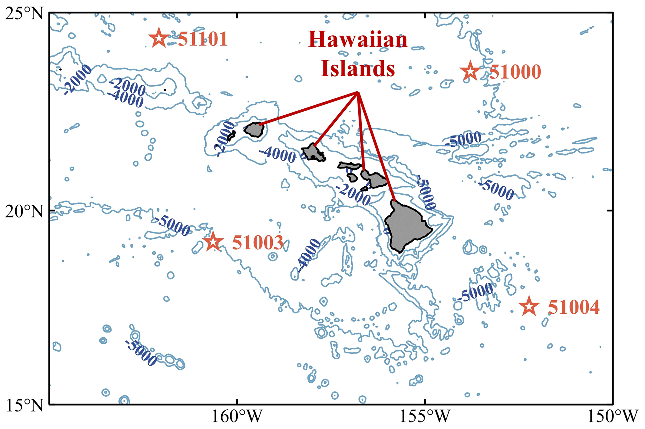
Figure 1 The geographical locations of the 51000, 51003, 51004, and 51101 NDBC buoys.

Table 1 Statistics of the geographical locations and water depth parameters of the selected NDBC buoys.

2.2 Dataset partitioning and feature selection

Waves depend on previous wave height, sea surface temperature, sea temperature, wind direction, wind speed, and pressure (Kamranzad et al., 2011; Nitsure et al., 2012; Fan et al., 2020). Because the buoy data have missing values, after data filtering, the research selected data longer than 2 years at each buoy as the training datasets to capture the year-round characteristics of wave parameters. The divisions and statistical characteristics of the training and testing datasets for the four buoys are shown in Table 2 and Fig. 2.

Table 2 NDBC dataset division and statistical information.

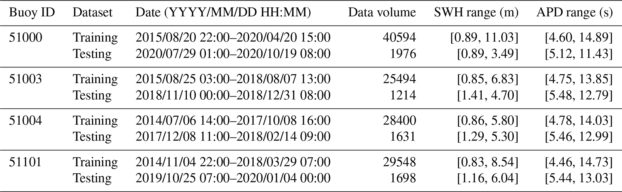
Figure 2 Statistical analysis of SWH and APD on the training and testing datasets of the four NDBC buoys.

The research selected SWH and APD, two wave parameters, as forecasting variables. The correlation between various environmental parameters with SWH and APD was determined by calculating Pearson correlation coefficients between the above parameters before selecting the input features. For the parameters X and Y, the Pearson correlation coefficients are calculated as follows.

$$\begin{array}{}\text{(1)}& r={\displaystyle \frac{\mathrm{cov}(X,Y)}{{\mathit{\sigma }}_X{\mathit{\sigma }}_Y}}={\displaystyle \frac{\frac{\mathrm{1}}{n}{\sum }_{i=\mathrm{1}}^n(X_i-\stackrel{\mathrm{‾}}{X})(Y_i-\stackrel{\mathrm{‾}}{Y})}{\sqrt{\frac{\mathrm{1}}{n}{\sum }_{i=\mathrm{1}}^n(X_i-\stackrel{\mathrm{‾}}{X}{)}^{\mathrm{2}}}\sqrt{\frac{\mathrm{1}}{n}{\sum }_{i=\mathrm{1}}^n(Y_i-\stackrel{\mathrm{‾}}{Y}{)}^{\mathrm{2}}}}}\end{array}$$

The Pearson correlation coefficients between SWH, MWD, WSPD, GST, WDIR, PRES, WTMP, ATMP, APD, and DPD were calculated after neglecting the parameter values at unrecorded moments (Fig. 3). As shown in Fig. 3, SWH has a positive correlation with APD, DPD, MWD, WSPD, GST, WDIR, and PRES to different degrees, and SWH has a negative correlation with WTMP and ATMP. Among them, WSPD and GST have a strong correlation (r=0.988), WTMP and ATMP have a strong correlation (r=0.901), and APD is considered to contain the main features of DPD. In order to utilize as many features of different physical parameters as possible while minimizing the computational redundancy, seven physical parameters – SWH, APD, MWD, WSPD, WDIR, PRES, and ATMP – were selected as input and training data for SWH and APD forecasting in the study.

2.3 Data pre-processing

Wind and wave directions are continuous in space but discontinuous numerically. For example, the directions 2^∘ and 358^∘ are very close, but the magnitude of the values differs significantly. Therefore, the wind and wave directions need to be pre-processed. The following formula recalculates the wind and wave directions (Nitsure et al., 2012).

$$\begin{array}{}\text{(2)}& \mathit{\psi }=\left\{\begin{array}{l}\mathrm{1}-\frac{\mathit{\theta }}{\mathrm{180}},\text{if}\mathrm{0}{}^{\circ }\le \mathit{\theta }\le \mathrm{180}{}^{\circ }\\ \frac{\mathit{\theta }-\mathrm{180}}{\mathrm{180}},\text{if}\mathrm{180}{}^{\circ }<\mathit{\theta }<\mathrm{360}{}^{\circ }\end{array}\right.,\end{array}$$

where θ is the original wind or wave directions, and ψ is the re-encoded value of wind or wave directions. ψ has a range of values from 0 to 1.

Since different NDBC physical variables have different units and magnitudes, this can substantially influence the performance of the neural network model. Therefore, each variable must be normalized or standardized before using it as input data for the model (X. Li et al., 2022). The research used a min–max normalization function to scale the input data between 0 and 1, which is calculated as follows.

$$\begin{array}{}\text{(3)}& x_{\mathrm{n}}={\displaystyle \frac{x-min\left(x\right)}{max\left(x\right)-min\left(x\right)}},\end{array}$$

where x_n is the normalized feature value, and x is the measured feature value.

3 Methods

3.1 Variational mode decomposition (VMD)

The VMD is an adaptive, completely non-recurrent mode variation and signal processing technique that combines the Wiener filter, the Hilbert transform, and the alternating direction method of multipliers (ADMM) technique (Dragomiretskiy and Zosso, 2014). VMD can determine the number of mode decompositions for a given sequence according to the situation. It has resolved the issues of mode mixing and boundary effects of EMD. The VMD decomposes the original sequence signal into an intrinsic mode function (IMF) of finite bandwidth, where the frequencies of each mode component u_k are concentrated around a central frequency ω_k. The VMD algorithm can be found in more detail in Appendix A.

3.2 Temporal convolutional networks (TCNs)

The TCN is a variant of the convolutional neural networks (CNNs) (Fig. 4). The TCN model uses causal convolution, dilated convolution, and residual blocks to extract sequence data with a large receptive field and temporality (Yan et al., 2020). The TCN performs convolution in the time domain (Kok et al., 2020), which has a more lightweight network structure than CNNs, LSTM, and GRU (gated recurrent unit; Bai et al., 2018). The TCN has the following advantages: (1) causal convolution prevents the disclosure of future information, (2) dilated convolution extends the receptive field of the structure, and (3) residual blocks maintain the historical information for a longer period.

Causal convolution is the most important part of TCN, where “causal” indicates that the output y_t (Fig. 4) at the time t is only dependent on the input x₁, x₂, …, x_t and is not influenced by x_t+1, x_t+2, …, x_T. The receptive field depends on the filter size and the network depth. However, the increase in filter size and network depth brings the risk of gradient disappearance and explosion. To avoid these problems, the TCN introduces dilated convolution based on causal convolution (Zhang et al., 2019). The dilated convolution introduces a dilation factor to adjust the receptive field. The processing capability of long sequences depends on the filter size, dilation factor, and network depth. The TCN effectively increases the receptive field without additional computational cost by increasing the dilation factor. To ensure training efficiency, the TCN introduces multiple residual blocks to accelerate the prediction model. Each residual block comprises two dilated causal convolution layers with the same dilation factor, normalization layer, ReLU (rectified linear unit) activation, and dropout layer. The input of each residual block is also added to the output when the input and output channels are different.

3.3 Long short-term memory (LSTM) networks

The traditional RNN is exposed to gradient explosion and vanishing risk. The LSTM network learns to reset itself at the appropriate time by adding a forgetting gate in RNNs, which releases internal resources. Meanwhile, LSTM learns faster by adding the self-looping method to generate a long-term continuous flow path. As a specific RNN, the LSTM network structure includes an input layer, a hidden layer, and an output layer. The structure of the LSTM cell is shown in Fig. 5. The LSTM can be found in more detail in Appendix B.

Figure 3 Pearson correlation coefficients between various physical parameters in NDBC data.

Figure 4 Structure of temporal convolutional networks.

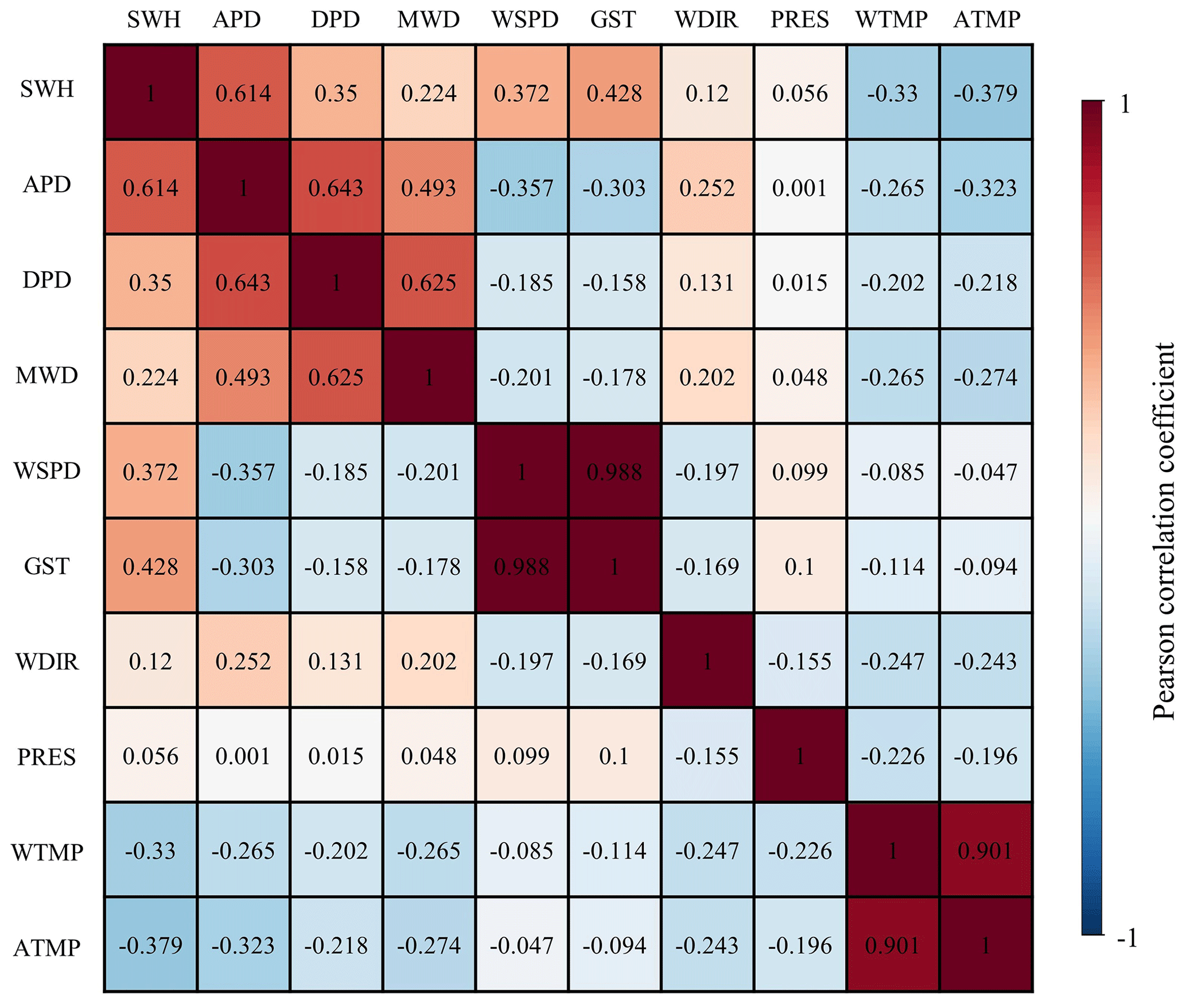
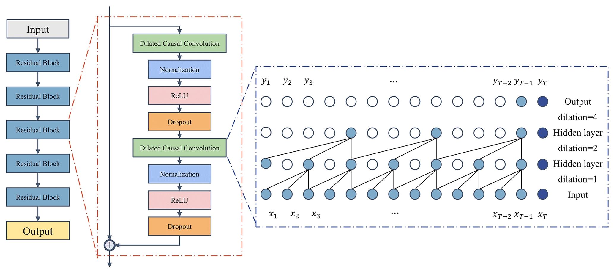
Figure 5 Structure of long short-term memory networks. The x_t denotes the current input vector, f_t is the forget gate, i_t is the input gate, c_t is the storage cell state, o_t is the output gate, h_t is the storage cell value at time t, σ is the sigmoid function, tanh denotes the hyperbolic tangent function, and “⊙” denotes the Hadamard matrix product.

3.4 Bayesian optimization (BO)

The BO aims to find the global maximizer (or minimizer) of the unknown objective function f(x) (Frazier, 2018), as shown as follows:

$$\begin{array}{}\text{(4)}& x^{\ast }=\begin{array}{c}\left(\text{arg max}f\right(x\left)\right)\\ x\mathit{ϵ}D\end{array},\end{array}$$

where D denotes the search space of x, where each dimension is a hyperparameter.

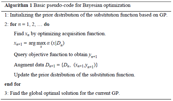
The BO has two critical components: first establishing an agency model of the objective function through a regression model (e.g., Gaussian process regression) and subsequently using the acquisition function to decide where to sample next (Frazier, 2018).

The Gaussian process (GP) is an extension of multivariate Gaussian distribution into an infinite-dimension stochastic process (Frazier, 2018; Brochu et al., 2010), which is the prior distribution of stochastic processes and functions. Any finite subset of random variables has a multivariate Gaussian distribution, and a GP is entirely defined by its mean function and covariance function (Rasmussen, 2004). BO optimizes the unknown function f(x) by combining the prior distribution of the function based on the GP with the current sample information to obtain the posterior of the function. The BO uses the expected improvement (EI) function as the acquisition function to evaluate the utility of the model posterior to determine the next input point. Let $f_{\mathrm{n}}^{\ast }$ be the optimal value of the acquisition function at the current iteration. The BO employs GP and EI in the iterations to evaluate and obtain the global optimal hyperparameters (Zhang et al., 2020a). The framework of the Bayesian parameter optimization algorithm is shown below.

4 Wave-parameter-prediction model framework and parameter settings

4.1 Data decomposition and parameter setting

The input to the VMD method requires the original signal f(t) and a predefined parameter K. The K determines the number of IMF patterns extracted during the decomposition. If the number of the extracted patterns is too large, it leads to a decrease in accuracy and unnecessary computational overhead (Liu et al., 2020). However, if the number of patterns is too small, the information in the patterns is insufficient to construct a high-precision prediction model. Therefore, it is essential to choose an appropriate one for K.

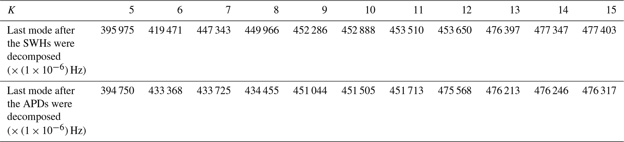
There is still a lack of general guidelines for the selection of the K parameter (Bisoi et al., 2019). Methods commonly used in other fields include the central frequency observation method (Hua et al., 2022; Chen et al., 2022; Fu et al., 2021), sample entropy (Zhang et al., 2020b; Niu et al., 2021), genetic algorithm (Huang et al., 2022), effective kurtosis index (Li et al., 2020), signal energy (Liu et al., 2020; Huang and Deng, 2021), etc. The central frequency observation method is convenient and effective, and it is used in this research to determine the number of patterns K for sequence decomposition. For various K parameter values, when the central frequency of the last mode has no significant changing trend, the number of K is currently the optimal number of mode decompositions. Table 3 calculates the central frequency of the last mode after the SWH and APD were decomposed with different K parameters; the optimal VMD decomposition mode number for SWH and APD is 13 and 12, respectively, when the variation in the central frequency is less than $\mathrm{1}\times {\mathrm{10}}^{-\mathrm{8}}$ Hz.

Table 3 The central frequency of the last mode after SWH and APD decomposition with different K parameters.

4.2 Wave-parameter-prediction model framework

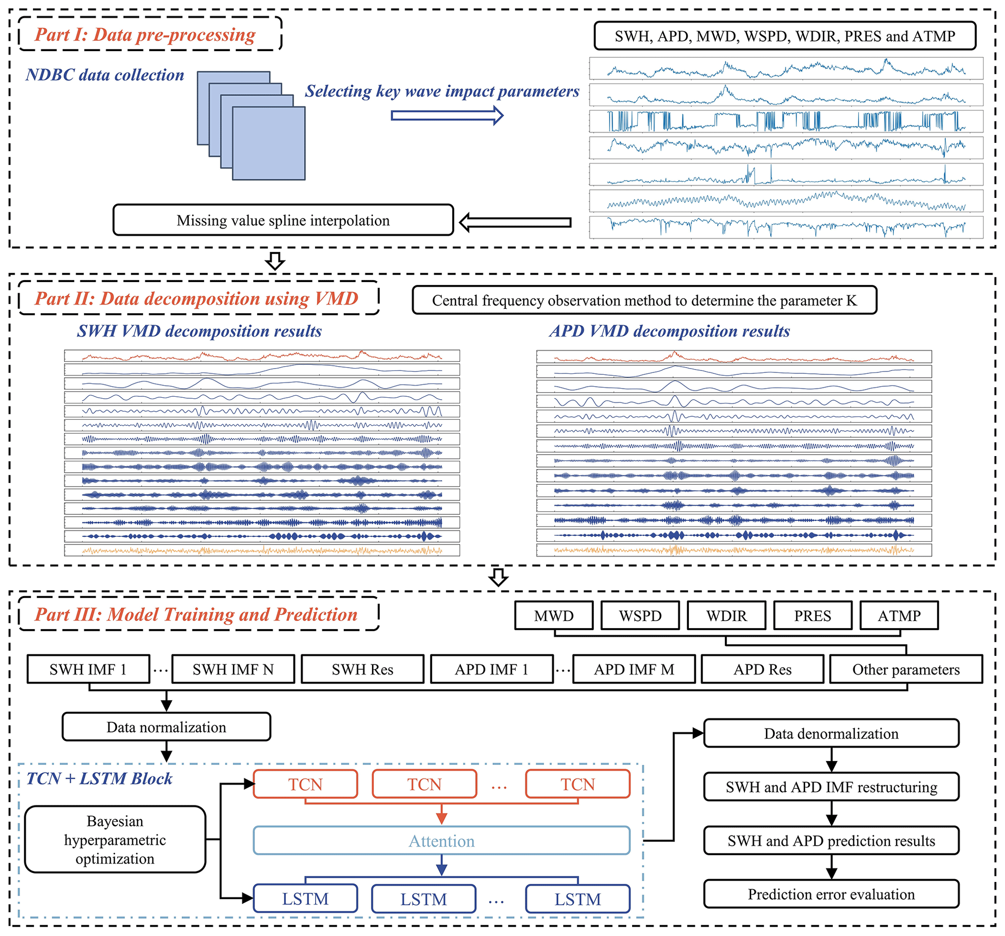
The overall structure of the VMD–TCN–LSTM wave-parameter-prediction model in the research is shown in Fig. 6, including three parts: data pre-processing, VMD data decomposition, and model training and forecasting. The input parameters to the model include 13 SWH IMFs and residuals; 12 APD IMFs and residual; original MWD, WSPD, PRES, and ATMP; and recoded WDIR. The lags of each input variable chosen for prediction are 3 h. The TCN cells and LSTM cells are used in the model to construct an encoder–decoder network with an attention mechanism to evaluate the accuracy of the VMD–TCN–LSTM model. The effect of the VMD technique and TCN cells on the forecasting results was also analyzed. The results of the VMD–TCN–LSTM model were compared with the VMD–LSTM and LSTM models. The VMD–LSTM model used both LSTM cells for encoding and decoding. The LSTM model uses data that have not been decomposed by VMD as input data. The LSTM model was also not encoded using TCN cells.

Figure 6 The overall structure of VMD–TCN–LSTM wave-parameter-prediction model.

4.3 Neural network hyperparameter optimization based on BO

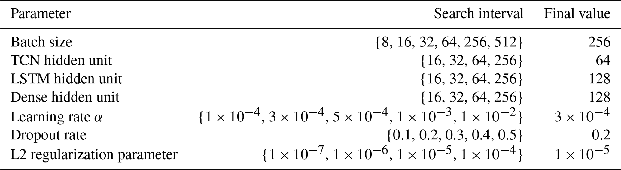
In the research, the BO algorithm is used to search for the optimal hyperparameters for the training of the VMD–TCN–LSTM model, including batch size, number of TCN hidden layer units, number of LSTM hidden layer units, number of dense hidden layer units, learning rate (α), dropout rate, and L2 regularization parameter of the LSTM layer. The hyperparameter search range and optimal results are shown in Table 4. Meanwhile, the learning rate decay and early-stopping method are used to prevent overfitting of the model and reduce the wasted training time.

Table 4 Bayesian hyperparameter optimization results.

5 Experiment and analysis

5.1 Evaluation metrics

To quantify the performance of the prediction model, the mean absolute error (MAE), root mean square error (RMSE), mean absolute percentage error (MAPE), and determination coefficient (R²) are used as evaluation metrics. The equations can be written as follows.

$$\begin{array}{}\text{(5)}& {\displaystyle }\mathrm{MAE}={\displaystyle \frac{\mathrm{1}}{N}}{\sum }_{i=\mathrm{1}}^N\left|y_{p\left(i\right)}-y_{t\left(i\right)}\right|,\text{(6)}& {\displaystyle }\mathrm{RMSE}=\sqrt{{\displaystyle \frac{\mathrm{1}}{N}}{\sum }_{i=\mathrm{1}}^N(y_{p\left(i\right)}-y_{t\left(i\right)}{)}^{\mathrm{2}}},\text{(7)}& {\displaystyle }\mathrm{MAPE}={\displaystyle \frac{\mathrm{1}}{N}}{\sum }_{i=\mathrm{1}}^N{\displaystyle \frac{\left|y_{p\left(i\right)}-y_{t\left(i\right)}\right|}{y_{t\left(i\right)}}}\times \mathrm{100}\mathit{\%},\text{(8)}& {\displaystyle }{R}^{\mathrm{2}}=\mathrm{1}-{\displaystyle \frac{{\sum }_{i=\mathrm{1}}^N(y_{p\left(i\right)}-y_{t\left(i\right)}{)}^{\mathrm{2}}}{{\sum }_{i=\mathrm{1}}^N(y_{t\left(i\right)}-{\stackrel{\mathrm{‾}}{y}}_t{)}^{\mathrm{2}}}},\end{array}$$

where N denotes the time length of the series data, y_t(i) is the true observation values of NDBC, y_p(i) is the predicted value, and ${\stackrel{\mathrm{‾}}{y}}_t$ is the average of the true observation values.

Furthermore, to quantify the improvement of the VMD technique and the TCN unit on the model accuracy, respectively, four parameters – I_MAE, I_RMSE, I_MAPE, and $I_{R^{\mathrm{2}}}$ (Eqs. 9 to 12, Table 4) – are introduced to compare the percentage improvement of the evaluation metrics of the VMD–LSTM and VMD–TCN–LSTM models concerning the LSTM model.

$$\begin{array}{}\text{(9)}& {\displaystyle }{I}_{\mathrm{MAE}}={\displaystyle \frac{{\mathrm{MAE}}_{\mathrm{LSTM}}-{\mathrm{MAE}}_{\mathrm{model}}}{{\mathrm{MAE}}_{\mathrm{LSTM}}}}\times \mathrm{100}\mathit{\%},\text{(10)}& {\displaystyle }{I}_{\mathrm{RMSE}}={\displaystyle \frac{{\mathrm{RMSE}}_{\mathrm{LSTM}}-{\mathrm{RMSE}}_{\mathrm{model}}}{{\mathrm{RMSE}}_{\mathrm{LSTM}}}}\times \mathrm{100}\mathit{\%},\text{(11)}& {\displaystyle }{I}_{\mathrm{MAPE}}={\displaystyle \frac{{\mathrm{MAPE}}_{\mathrm{LSTM}}-{\mathrm{MAPE}}_{\mathrm{model}}}{{\mathrm{MAPE}}_{\mathrm{LSTM}}}}\times \mathrm{100}\mathit{\%},\text{(12)}& {\displaystyle }{I}_{R^{\mathrm{2}}}={\displaystyle \frac{R_{\mathrm{model}}^{\mathrm{2}}-R_{\mathrm{LSTM}}^{\mathrm{2}}}{R_{\mathrm{LSTM}}^{\mathrm{2}}}}\times \mathrm{100}\mathit{\%},\end{array}$$

where the subscript “LSTM” represents the evaluation metrics of the LSTM model, and the subscript “model” represents the evaluation metrics of the VMD–LSTM or VMD–TCN–LSTM models.

5.2 Three-hour forecasting performance

The evaluation metrics of SWH and APD for different prediction models on the testing sets of the four buoys for the 3 h forecasts are shown in Table 5, where the best results are shown in bold. As shown in the table, both the VMD–LSTM and VMD–TCN–LSTM models significantly outperform the results of the LSTM model. This indicates that the data pre-processing method of VMD can extract the features of the sequence data well for the 3 h SWH and APD forecasts, which can significantly improve the forecasting performance. Meanwhile, the improvement of the TCN cells on the model performance is not particularly significant for the 3 h SWH and APD forecasts. The performance of the VMD–TCN–LSTM model was slightly better than that of the VMD–LSTM model only in some instances.

Table 5 Accuracy evaluation of the three models in 3 h SWH and APD forecasts. The best performances of the LSTM, VMD-LSTM, and VMD-TCN-LSTM models are shown in bold in the table.

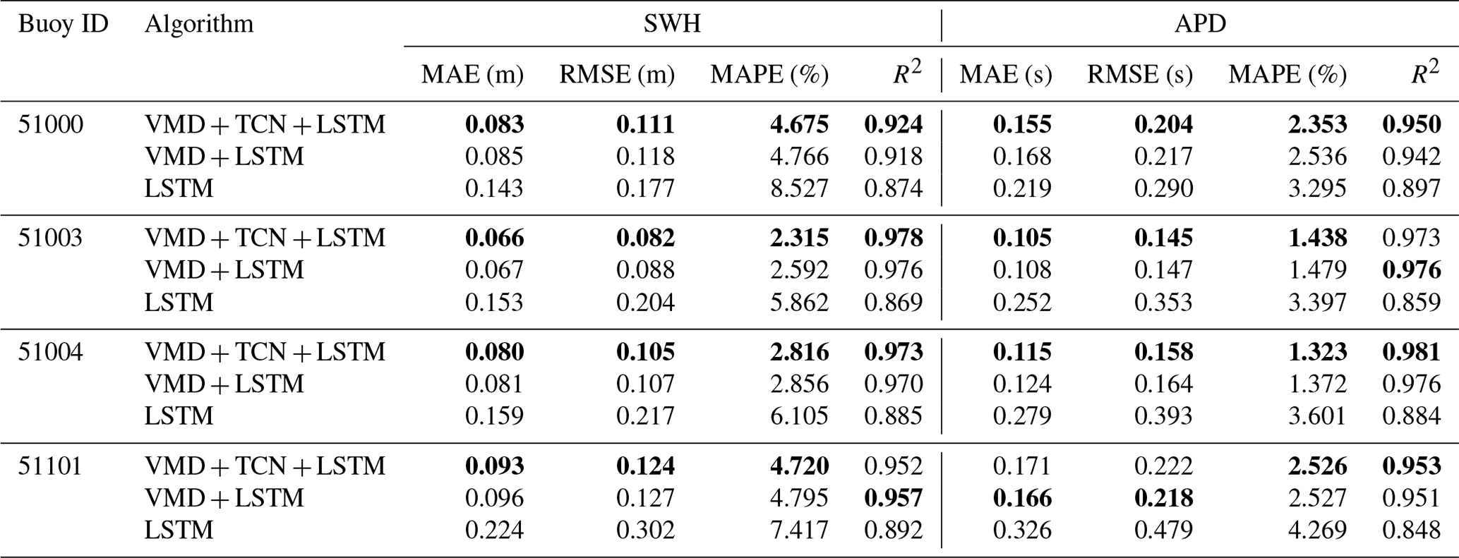
In the SWH forecasting at four buoys, the buoy with the best performance was buoy 51003, with MAE, RMSE, MAPE, and R² of 0.066 m, 0.082 m, 2.315 %, and 0.978, respectively. Among the APD forecasting at four buoys, the VMD–TCN–LSTM model had the smallest MAE and RMSE at buoy 51003, with 0.105 and 0.145 s, respectively, and the smallest MAPE and the highest R² at buoy 51004, with 1.323 % and 0.981, respectively.

To compare the forecasting results of different models more visually, Fig. 7 shows the comparison results of the 3 h SWH and APD forecasting curves of different models with the observed values for the first 24 h of the testing set for each buoy. As shown in Fig. 7, the forecasting results of VMD–TCN–LSTM have good agreement with the observed values of NDBC at most moments on all four buoys. The forecasting results of VMD–LSTM are also close to the observed values. Meanwhile, the results of both the VMD–TCN–LSTM and VMD–LSTM models are significantly better than those of the LSTM model. This shows that both the VMD–TCN–LSTM and VMD–LSTM models can better capture the time-varying characteristics of wave series data and thus perform well in the SWH and APD forecasts.

Figure 7 Comparison results of the 3 h SWH and APD forecasting curves of different models with the observed values for the first 24 h of the testing datasets for each buoy.

Figure 8 shows the linear-fitting results of the SWH and APD observations with the forecasts of the three models for each buoy. According to the linear-fitting formula, the fitting curves of both the VMD–LSTM and VMD–TCN–LSTM models were closer to “y=x” compared to the LSTM model. For the 3 h SWH forecasts, the fitted formula of the VMD–TCN–LSTM forecasting results for buoy 51004 was closest to y=x, which had a slope of 0.9817 and an intercept of 0.0404 (Fig. 8e). For the 3 h APD forecasts, the fitted formula of the VMD–TCN–LSTM forecasting results for buoy 51004 was closest to y=x, which had a slope of 0.9929 and an intercept of 0.0829 (Fig. 8f). The results indicate that the forecasting performance of these two models is significantly better than that of the LSTM model, which is consistent with the findings in Fig. 7 and Table 5.

Figure 8 The linear fitting of the 3 h SWH and APD predictions and observations for the three models.

Meanwhile, the SWH and APD of the four buoys have different ranges of values and other statistical features, which proves that the two models, VMD–LSTM and VMD–TCN–LSTM, have good robustness for SWH and APD forecasting under different scenarios. The VMD technique can extract the time-varying features of the original data, contributing to the accuracy of the prediction model. In addition, using TCN cells instead of LSTM cells for encoding the network model can also reduce the error in the prediction model by a small amount.

5.3 Twelve-hour forecasting performance

The evaluation metrics of SWH and APD for different prediction models on the testing sets of the four buoys for the 12 h forecasts are shown in Table 6, and the best results are shown in bold in the table. As shown in Table 6, both the VMD–LSTM and VMD–TCN–LSTM models significantly outperform the performances of the LSTM model. This is like the results of the 3 h SWH and APD forecasts.

In addition, the performances of the VMD–TCN–LSTM model outperformed the VMD–LSTM for the SWH and APD forecasts at all buoys. Compared with the 3 h forecasts, the TCN cells were more significant for the model performance improvement in the 12 h wave forecasts. This is because the residual block structure used in the TCN cells can maintain the historical information for a long time. The TCN cells are more significant in the longer time wave parameter forecasts.

Among the SWH forecasting of the four buoys, the VMD–TCN–LSTM model had the smallest MAE and RMSE at buoy 51000, with 0.125 and 0.165 m, respectively. Buoy 51003 had the smallest MAPE of 5.912 %. Buoy 51004 had the largest R² of 0.898. In the APD forecasting at four buoys, the VMD–TCN–LSTM model had the smallest MAE and RMSE at buoy 51003, with 0.247 and 0.336 s, respectively, and the smallest MAPE and the highest R² at buoy 51004, with 3.329 % and 0.904, respectively.

The comparison of the forecasting curves of different models with the observations of NDBC for the first 24 h of the testing set of the four NDBC buoys for the 12 h SWH and APD forecasts is shown in Fig. 9. As shown in the figure, the forecasts of the VMD–TCN–LSTM model were in excellent agreement with the NDBC observations for most moments at all four buoys, and it significantly outperforms the forecasting curves of the VMD–LSTM and LSTM models. The results show that the VMD–TCN–LSTM model can better capture the time-varying characteristics of wave series data and thus performs well in forecasting SWH and APD.

Table 6 Accuracy evaluation of the three models in 12 h SWH and APD forecasts. The best performances of the LSTM, VMD-LSTM, and VMD-TCN-LSTM models are shown in bold in the table.

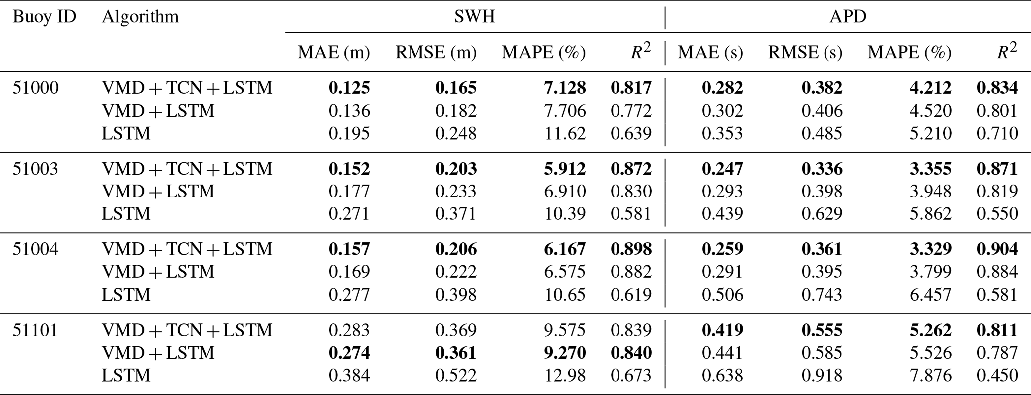
Figure 9 Comparison results of the 12 h SWH and APD forecasting curves of different models with the observed values for the first 24 h of the testing datasets for each buoy.

Figure 10 shows the linear-fitting results for the 12 h SWH and APD forecast data and observations at each buoy for the three models. As shown in Fig. 10, it was evident that the forecasting results of the VMD–TCN–LSTM model have the closest-fitting formula to y=x compared with the LSTM model, and the VMD–TCN–LSTM model is better than the VMD–LSTM model. In the 12 h SWH forecasts, the fitted formula of the VMD–TCN–LSTM forecasting results for buoy 51000 was closest to y=x, which had a slope of 0.9256 and an intercept of 0.1252 (Fig. 10a). Among the 12 h APD forecasts, the fitted formula of the VMD–TCN–LSTM forecasting results for buoy 51004 was closest to y=x, which had a slope of 0.9664 and an intercept of 0.2500 (Fig. 10f). Both the VMD–TCN–LSTM and VMD–LSTM models have significantly better forecasting performance than the LSTM model. This is consistent with the conclusions of Fig. 9 and Table 6.

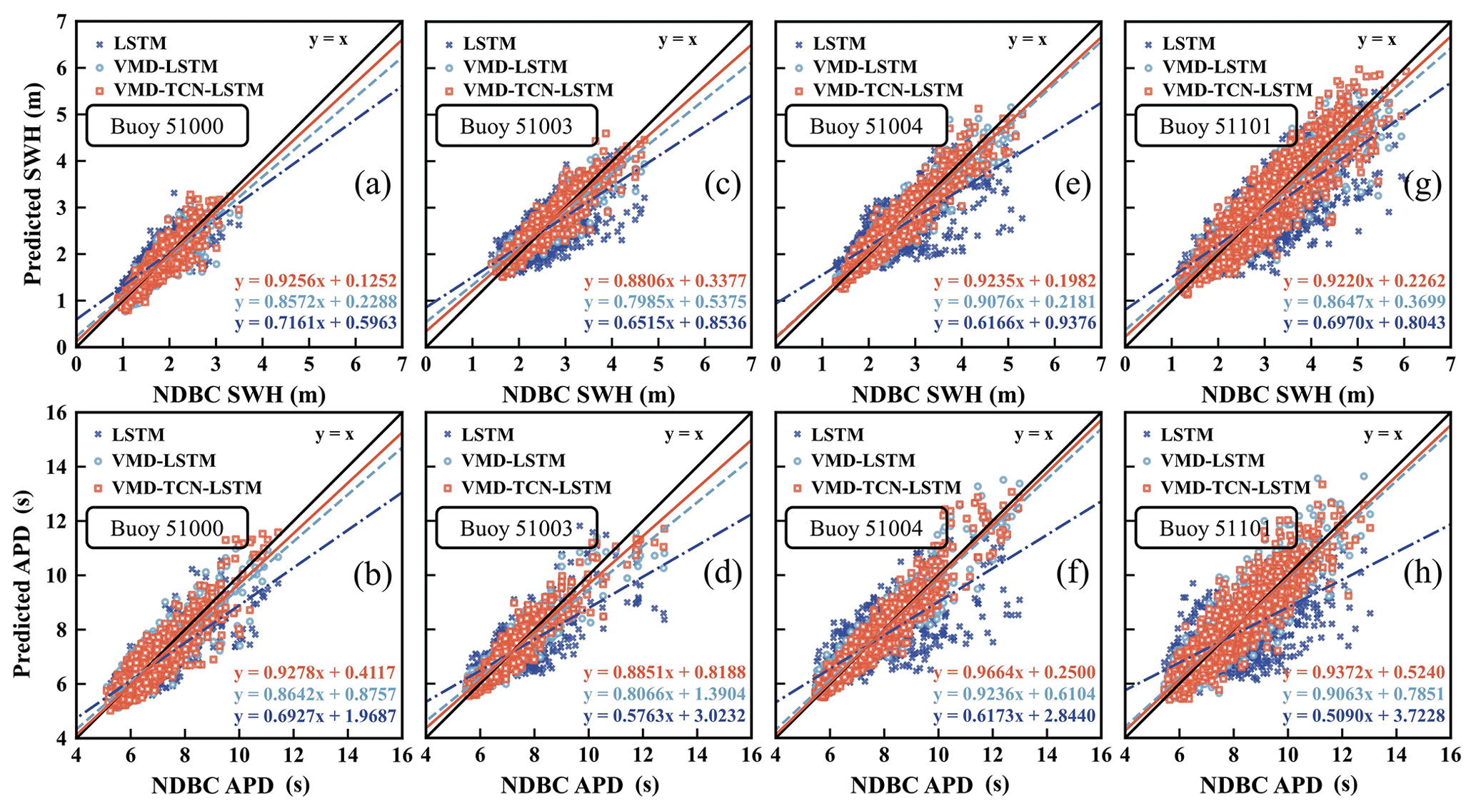
Figure 10 The linear fitting of the 12 h SWH and APD predictions and observations for the three models.

Moreover, the variability in the numerical ranges of SWH and APD for the four buoys also demonstrates the excellent robustness of the VMD–TCN–LSTM model for SWH and APD forecasts in different scenarios. The pre-processing of wave sequence data using VMD can extract the time-varying features of the original data well, and the expansion convolution module of TCNs increases the perceptual field of the model. At the same time, the residual block enables the preservation of the long-term information of the original data. Therefore, the hybrid model of VMD, TCNs, and LSTM can significantly improve the accuracy of the forecasting results.

5.4 Twenty-four- and forty-eight-hour forecasting performance

To further compare the performance of the VMD–TCN–LSTM model for the longer time wave forecasts, the error indices of the prediction models at 24 and 48 h are presented in Table 7 and Table 8, respectively, where the best results are shown in bold in the table.

Table 7 Accuracy evaluation of the three models in 24 h SWH and APD forecasts. The best performances of the LSTM, VMD-LSTM, and VMD-TCN-LSTM models are shown in bold in the table.

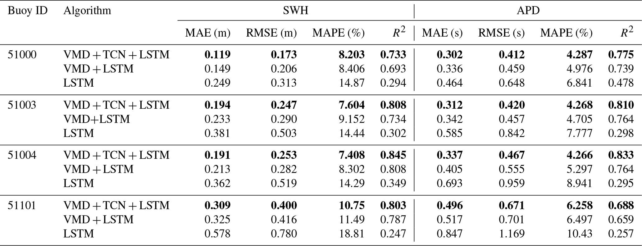
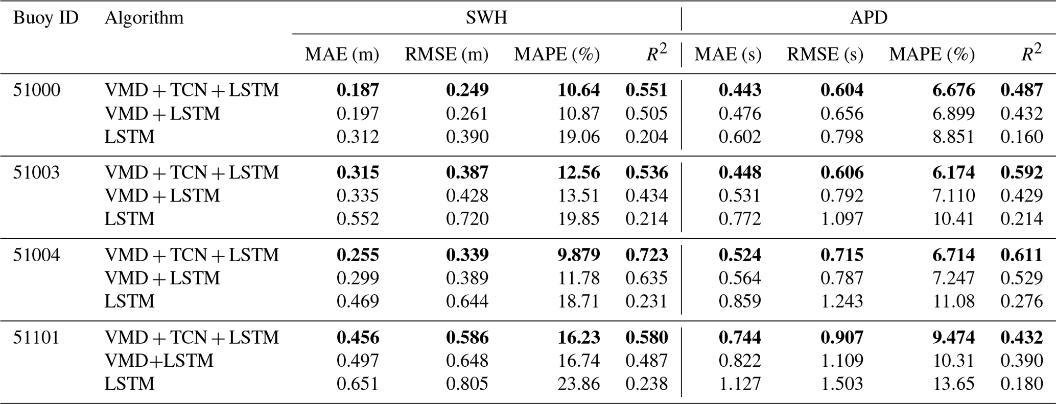
Table 8 Accuracy evaluation of the three models in 48 h SWH and APD forecasts. The best performances of the LSTM, VMD-LSTM, and VMD-TCN-LSTM models are shown in bold in the table.

As shown in Table 7, for the 24 h forecasts, the MAE and RMSE for the forecasting of SWH and APD at buoy 51000 are the lowest, with MAE of 0.119 m and 0.302 s and RMSE of 0.173 m and 0.412 s, respectively. This is because the range of data for SWH and APD in the testing datasets at buoy 51000 is the smallest (Fig. 2). At buoy 51004, the forecasting of SWH and APD had the lowest MAPE and the highest R², with MAPE of 7.408 % and 4.266 % and R² of 0.845 and 0.833, respectively.

As shown in Table 8, for the 48 h forecasts, the MAE and RMSE for the forecasting of SWH and APD at buoy 51000 are the lowest, with MAE of 0.187 m and 0.443 s and RMSE of 0.249 m and 0.604 s, respectively. It showed a similar performance to the 24 h SWH and APD forecasts. Buoy 51004 had the lowest R², with 0.723 and 0.611 for SWH and APD forecasts, respectively. Buoy 51004 also had a low MAPE of 9.879 % for the SWH forecasts. Buoy 51003 had a low MAPE of 6.174 % for the APD forecasts.

5.5 Analysis of improvement of VMD–TCN–LSTM compared with previous models

To precisely quantify the prediction performance improvement rate of the VMD technique and TCN cells for the LSTM model, we need to analyze them separately. The model performance improvement rates for VMD–TCN–LSTM and VMD–LSTM were calculated by using Eq. (9) to Eq. (12) (Table 9), and bold in the table represents the highest result of the model performance improvement rate. As shown in Table 9, the VMD–LSTM and VMD–TCN–LSTM models had very similar improvement rates in MAE, RMSE, MAPE, and R² in the 3 h SWH forecasts, which indicates that the improvement of the VMD–TCN–LSTM model for prediction accuracy in the 3 h SWH forecasts is mainly contributed by the VMD technique. The same conclusion can be obtained in the 3 h APD forecasts. Subsequently, when the length of forecasting increases to 12, 24, and 48 h, the TCN cells are more significant for the decrease in MAE, RMSE, and MAPE and the increase in R² for the forecasting results.

Table 9 The performance improvement rate of the VMD–TCN–LSTM and VMD–LSTM models relative to the LSTM model. The best performances of the LSTM, VMD-LSTM, and VMD-TCN-LSTM models are shown in bold in the table.

There was no significant rule for the decreased rate of TCN cells for the MAE, RMSE, and MAPE of the model at various forecasting time lengths. However, the contribution of TCN cells to the improvement of R² for forecasting results gradually increases with the increase in forecasting time length. It reaches the maximum value in the 48 h SWH and APD forecasts. As shown in Table 9, in the 48 h SWH forecasts, the VMD technique increases the R² of the forecasting performance by 132.5 %, and the TCN cells for model encoding resulted in a further 36.8 % improvement in the R² of the model. In the 48 h APD forecasts, the VMD technique increases the R² of the forecasting performance by 119.7 %. The TCN cells resulted in a further 40.9 % improvement in the R² of the model.

LSTM has advantages in solving the prediction problem by using time series data and has been widely used in many fields. However, due to the strong non-linear effects in the generation and evolution of waves, the wave prediction model that only uses LSTM will weaken the ability of generalization. As a result, both the model's ability to adapt to new samples and its prediction accuracy will be reduced. The VMD signal decomposition method can effectively extract the features of the original wave data, which can enhance LSTM's ability to capture the long-term dependence of the time series data and further improve the performance of the wave prediction model. This study shows that the VMD can significantly reduce the model's MAE, RMSE, and MAPE and improve the model's R². The TCN introduces multiple residual blocks to speed up the forecast model and can retain historical wave change information over long periods. This study also shows that the TCN's impact increases as the forecast period lengthens. The proposed hybrid VMD–TCN–LSTM shows its advantage in predicting both the wave height and the wave period. This method could also be used in other fields which have similar non-linear features to waves.

6 Conclusions

This paper proposes a hybrid VMD–TCN–LSTM model for forecasting SWH and APD using buoy data near the Hawaiian Islands provided by the NDBC. Seven physical parameters – SWH, APD, MWD, WSPD, WDIR, PRES, and ATMP – were chosen for training the prediction model in the research. Specifically, the original features of the non-smooth wave series data were extracted by decomposing the original SWH and APD series data using the VMD technique. Subsequently, a prediction model is constructed using a network structure encoded by TCN cells and decoded by LSTM cells, where the TCN cells can capture the local feature information of the original series and can maintain the historical information for a long time. Simultaneously, the BO algorithm is used to obtain the optimal hyperparameters of the model to prevent overfitting or underfitting problems of the model. Ultimately, the 3, 12, 24, and 48 h forecasts of SWH and APD were implemented based on the VMD–TCN–LSTM model. In addition, eight evaluation metrics – MAE, RMSE, MAPE, R², I_MAE, I_RMSE, I_MAPE, and $I_{R^{\mathrm{2}}}$ – were used to evaluate and test the model performance.

The VMD–TCN–LSTM model proposed in this research outperforms the LSTM and the VMD–LSTM models for all forecasting time lengths at all four NDBC buoys. This demonstrates that the VMD–TCN–LSTM model has good robustness and generalization ability. For the 3 h SWH and APD forecasts, the improvement of the hybrid model for forecasting accuracy is mainly contributed by the VMD technique, and the contribution of the TCN cells to the advancement of the model accuracy is relatively tiny. Subsequently, the contribution of TCN cells to improve model forecasting accuracy was gradually significant when the forecasting time length increased to 12, 24, and 48 h.

There was no significant rule for the decreased rate of TCN cells for the MAE, RMSE, and MAPE of the model at various forecasting time lengths. The contribution of TCN cells to improving R² for forecasting results gradually increases with the increase in forecasting time length. The VMD technique and the TCN cells improved the R² of the model by 132.5 % and 36.8 %, respectively, in the 48 h SWH forecasts. In the 48 h APD forecasts, the VMD technique and the TCN cells improved the R² of the model by 119.7 % and 40.9 %, respectively.

Now that the short-term SWH and APD can be accurately predicted using the hybrid VMD–TCN–LSTM, this method would be useful for some marine-related activities which are highly dependent on wave height and period predictions, such as ocean-wave-energy projects, shipping, fishing, coastal structures, and naval operations. Future work will investigate the effect of different driving data on the prediction skill or the use of VMD–TCN–LSTM to predict other marine environmental parameters (e.g., sea level or winds). The combination of numerical wave models and the VMD–TCN–LSTM for large-scale SWH and APD simulations will also be developed.

Appendix A: Detailed description of the VMD algorithm

The nucleus of VMD is the construction and solution of the variational problem, which is essentially a constrained optimization problem. The variational problem is to minimize the sum of the estimated bandwidths of the IMFs, with the constraint that the sum of the IMFs is the original signal. The calculation formula is as follows:

$$\begin{array}{}\text{(A1)}& \begin{array}{rl}& \begin{array}{c}\min \\ \mathit{\left\{}{u}_k\mathit{\right\}},\mathit{\left\{}{\mathit{\omega }}_k\mathit{\right\}}\end{array}\mathit{\left\{}{\sum }_k{∥{\partial }_t\left[{\left(\mathit{\delta }\left(t\right)+{\displaystyle \frac{j}{\mathit{\pi }t}}\right)}^{\ast }{u}_k\left(t\right)\right]e^{-j{\mathit{\omega }}_{k}t}∥}_{\mathrm{2}}^{\mathrm{2}}\mathit{\right\}}\\ & \mathrm{s}.\mathrm{t}.{\sum }_k{u}_k=f,\end{array}\end{array}$$

where “s.t.” is the abbreviation of “subject to”; {u_k}:= {u₁, u₂, …, u_k} and {ω_k}:={ω₁, ω₂, …, ω_k} denote the set of all modes and their corresponding central frequencies, respectively. The f is the original signal, k is the total number of modes, and δ(t) represents the Dirac distribution. The j is an imaginary unit, and “^∗” denotes the convolution.

To simplify the above equations, VMD introduces a quadratic penalty term (α) and Lagrange multipliers (λ) to convert the constrained problem into a non-constrained problem; α guarantees the reconstruction accuracy of the signal, and λ maintains the constraint stringency.

$$\begin{array}{}\text{(A2)}& \begin{array}{rl}& \mathcal{L}\left(\mathit{\left\{}{u}_k{\mathit{\omega }}_k\mathit{\right\}},\mathit{\lambda }\right):=\mathit{\alpha }{\sum }_k{∥{\partial }_t\left[{\left(\mathit{\delta }\left(t\right)+{\displaystyle \frac{j}{\mathit{\pi }t}}\right)}^{\ast }{u}_k\left(t\right)\right]e^{-j{\mathit{\omega }}_{k}t}∥}_{\mathrm{2}}^{\mathrm{2}}\\ & +{∥f\left(t\right)-{\sum }_k{u}_k\left(t\right)∥}_{\mathrm{2}}^{\mathrm{2}}+〈\mathit{\lambda }\left(t\right),f\left(t\right)-{\sum }_k{u}_k\left(t\right)〉\end{array}\end{array}$$

Finally, the ADMM solves the saddle point of the augmented Lagrange multiplier. Update the iterative formulas for u_k, ω_k, and λ as follows.

$$\begin{array}{}\text{(A3)}& {\displaystyle }{\widehat{u}}_k^{n+\mathrm{1}}\left(\mathit{\omega }\right)={\displaystyle \frac{\widehat{f}\left(\mathit{\omega }\right)-{\sum }_{i\ne k}{\widehat{u}}_i\left(\mathit{\omega }\right)+\frac{\widehat{\mathit{\lambda }}\left(\mathit{\omega }\right)}{\mathrm{2}}}{\mathrm{1}+\mathrm{2}\mathit{\alpha }{\left(\mathit{\omega }-{\mathit{\omega }}_k\right)}^{\mathrm{2}}}},\text{(A4)}& {\displaystyle }{\mathit{\omega }}_k^{n+\mathrm{1}}={\displaystyle \frac{{\int }_{\mathrm{0}}^{\mathrm{\infty }}\mathit{\omega }{\left|{\widehat{u}}_k\left(\mathit{\omega }\right)\right|}^{\mathrm{2}}d\mathit{\omega }}{{\int }_{\mathrm{0}}^{\mathrm{\infty }}{\left|{\widehat{u}}_k\left(\mathit{\omega }\right)\right|}^{\mathrm{2}}d\mathit{\omega }}},\text{(A5)}& {\displaystyle }{\widehat{\mathit{\lambda }}}^{n+\mathrm{1}}\left(\mathit{\omega }\right)={\widehat{\mathit{\lambda }}}^n\left(\mathit{\omega }\right)+\mathit{\tau }\left(\widehat{f}\left(\mathit{\omega }\right)-{\sum }_{k=\mathrm{1}}^K{\widehat{u}}_k^{n+\mathrm{1}}\left(\mathit{\omega }\right)\right),\end{array}$$

where $\widehat{f}\left(\mathit{\omega }\right)$, ${\widehat{u}}_k\left(\mathit{\omega }\right)$, $\widehat{\mathit{\lambda }}\left(\mathit{\omega }\right)$, and ${\widehat{u}}_k^{n+\mathrm{1}}\left(\mathit{\omega }\right)$ are the Fourier transforms of f(ω), u_k(ω), λ(ω), and $u_k^{n+\mathrm{1}}\left(\mathit{\omega }\right)$, respectively. The n and τ are the number of iterations and update coefficients of dual ascent. The iterations are stopped when the convergence condition satisfies the following equation.

$$\begin{array}{}\text{(A6)}& {\sum }_k{\displaystyle \frac{{∥{\widehat{u}}_k^{n+\mathrm{1}}-{\widehat{u}}_k^n∥}_{\mathrm{2}}^{\mathrm{2}}}{{∥{\widehat{u}}_k^n∥}_{\mathrm{2}}^{\mathrm{2}}}}<\mathit{ϵ}\end{array}$$

Appendix B: Detailed description of the LSTM

A LSTM cell consists of four components: the forget gate f_t, the input gate i_t, the storage cell state c_t, and the output gate o_t.

The f_t determines the number of memories that need to be reserved from c_t−1 to c_t.

$$\begin{array}{}\text{(B1)}& f_t=\mathit{\sigma }\left(W_f\cdot \left[x_t,h_{t-\mathrm{1}}\right]+b_f\right)\end{array}$$

The i_t determines the information that is input to this cell state.

$$\begin{array}{}\text{(B2)}& i_t=\mathit{\sigma }\left(W_i\cdot \left[x_t,h_{t-\mathrm{1}}\right]+b_i\right)\end{array}$$

The o_t represents the information output from this cell state.

$$\begin{array}{}\text{(B3)}& o_t=\mathit{\sigma }\left(W_o\cdot \left[x_t,h_{t-\mathrm{1}}\right]+b_o\right)\end{array}$$

The cell state is

$$\begin{array}{}\text{(B4)}& {\displaystyle }{C}_t=f_t\odot C_{t-\mathrm{1}}+i_t\odot {\stackrel{\mathrm{̃}}{C}}_t,\text{(B5)}& {\displaystyle }{\stackrel{\mathrm{̃}}{C}}_t=\tanh \left(W_c\cdot \left[x_t,h_{t-\mathrm{1}}\right]+b_c\right).\end{array}$$

The next cell with h_t is

$$\begin{array}{}\text{(B6)}& h_t=o_t\odot \tanh \left(C_t\right).\end{array}$$

In the above equation, x_t denotes the current input vector, and W and b denote the hyperparameters of the weights and biases. The h_t is the storage cell value at time t. The σ is the sigmoid function, tanh denotes the hyperbolic tangent function, “⋅” denotes the dot product of matrices, and “⊙” denotes the Hadamard matrix product of equidimensional matrices (Yu et al., 2019; Gers et al., 2000; Hochreiter and Schmidhuber, 1997). The sigmoid function takes values in the range of [0, 1], and in the forgetting gate, if the value is 0, the information of the previous state is completely forgotten, and if the value is 1, the information is completely retained. The tanh function takes the values in the range of [−1, 1].