On the ocean's response to enhanced Greenland runoff in model experiments: relevance of mesoscale dynamics and atmospheric coupling

Increasing Greenland Ice Sheet melting is anticipated to impact water mass transformation in the subpolar North Atlantic and ultimately the meridional overturning circulation. Complex ocean and climate models are widely applied to estimate magnitude and timing of related impacts under global warming. We discuss the role of the ocean mean state, subpolar water mass transformation, mesoscale eddies, and atmospheric coupling in shaping the response of the subpolar North Atlantic Ocean to enhanced Greenland runoff. In a suite of eight dedicated 60- to 100-year-long model experiments with and without atmospheric coupling, with eddy processes parameterized and explicitly simulated and with regular and significantly enlarged Greenland runoff, we find (1) a major impact by the interactive atmosphere in enabling a compensating temperature feedback, (2) a non-negligible influence by the ocean mean state biased towards greater stability in the coupled simulations, both of which make the Atlantic meridional overturning circulation less susceptible to the freshwater perturbation applied, and (3) a more even spreading and deeper mixing of the runoff tracer in the subpolar North Atlantic and enhanced inter-gyre exchange with the subtropics in the strongly eddying simulations. Overall, our experiments demonstrate the important role of mesoscale ocean dynamics and atmosphere feedback in projections of the climate system response to enhanced Greenland Ice Sheet melting and hence underline the necessity to advance scale-aware eddy parameterizations for next-generation climate models.

1 Introduction

Water mass transformation in the subpolar North Atlantic (SPNA) plays a key role in the global thermohaline circulation. Warm and salty Atlantic water being transported northward by the Atlantic meridional overturning circulation (AMOC) cools as it loses heat to the atmosphere but also freshens by mixing with polar waters exported from the Arctic Ocean, coastal runoff, and precipitation. The AMOC strength is one of the major tipping elements in the climate system (Lenton et al., 2008, 2019; Drijfhout et al., 2015); its poleward heat transport is important to the inhabitability of northern Europe, as well as to Northern Hemisphere ice sheet growth and decay. A remnant of larger land ice areas, the present-day Greenland Ice Sheet (GrIS), still holds a freshwater mass equivalent to about 7.2 m of global sea-level rise, which qualifies the ice sheet as a tipping element itself (Lenton et al., 2008; Aschwanden et al., 2019). Observations and model-supported estimates show an acceleration of GrIS melting over the past couple of decades (Chen et al., 2006; Barletta et al., 2013; Mouginot et al., 2019; The IMBIE Team, 2020) so that the ice sheet's net mass balance was negative in each of the last 25 years (Polar Portal Season Report 2021, http://polarportal.dk, last access: 10 February 2023).

This led to an increase in freshwater flux from Greenland of almost 50 % from the mid-1990s to 2010 (Bamber et al., 2018). However, Greenland meltwater still makes a relatively small contribution to the SPNA freshwater budget considering Arctic Ocean export (Haine et al., 2015; Steur et al., 2018). Tracing glacial meltwater in Greenland's boundary currents and into the deep-water-formation regions is a major challenge requiring enormous observational effort, with some but limited recent success (Rhein et al., 2018; Huhn et al., 2021; Hendry et al., 2021).

Numerous model studies have demonstrated that enhanced mass loss by the GrIS has the potential to reduce the strength of the AMOC (e.g., Rahmstorf et al., 2005; Swingedouw et al., 2013; Jackson and Wood, 2018; Golledge et al., 2019). The additional freshwater spread across the SPNA stabilizes the water column, eventually limits overall heat loss in the eastern North Atlantic, inhibits deep convection, and thus reduces the amount and density of North Atlantic Deep Water being formed. Uncertainty remains regarding the true sensitivity of the AMOC to global warming and associated additional freshwater input from the GrIS (Rahmstorf et al., 2015; Bakker et al., 2016; Böning et al., 2016; Weijer et al., 2020). Availability of computing power restricts studies of millennial timescales to less comprehensive, non-eddying models (e.g., Rahmstorf et al., 2005; Hawkins et al., 2011), whereas models of full complexity applied to mesoscale-resolving grids are limited to multi-decadal applications (e.g., Böning et al., 2016; Dukhovskoy et al., 2019; Love et al., 2021). Comprehensive climate models consistently show a large-scale ocean circulation response on a multi-decadal timescale to sudden changes in Greenland meltwater runoff (Weijer et al., 2012; Swingedouw et al., 2013; Jackson and Wood, 2018; Martin et al., 2022). Mesoscale dynamic features, such as eddies and boundary currents, play a critical role in water mass transformation in the SPNA, where, for instance, eddies advect fresh polar water from the boundary into the central Labrador Sea and are crucial for the process of restratification after deep convection and thus need to be simulated or properly parameterized (Gelderloos et al., 2011; Böning et al., 2016; Rieck et al., 2019; Castelao et al., 2019; Georgiou et al., 2019; Tagklis et al., 2020; Pennelly and Myers, 2022). The implications of failing to correctly represent mesoscale processes in the deep-convection regions of the SPNA in GrIS-melt-related studies are not well quantified. In the present study, we aim to bridge the gap between most complex, eddy-rich ocean hindcasts (Böning et al., 2016) limited to the past few decades and comprehensive but non-eddying climate model simulations (Martin et al., 2022) typically applied to idealized freshwater scenarios for centennial projections or millennial paleo-applications.

We conduct a freshwater-release experiment of 0.05 Sv enhanced runoff from Greenland using a hierarchy of model configurations. The magnitude of this perturbation is less than in traditional hosing experiments (≥ 0.1 Sv; e.g., Stouffer et al., 2006; Gerdes et al., 2006; Hu et al., 2011; Weijer et al., 2012; Swingedouw et al., 2013; Jackson and Wood, 2018) and within the range of estimates for the end of the 21st century using linear-trend extrapolation (0.06–0.08 Sv; Bamber et al., 2018; The IMBIE Team, 2020) or sophisticated ice sheet modeling of global warming effects under the Representative Concentration Pathway (RCP) 8.5 scenario (0.018–0.075 Sv; Golledge et al., 2019; Goelzer et al., 2020). For comparison, the imbalance in GrIS mass over the past 2 decades equals an average runoff increase of 0.007–0.008 Sv (Bamber et al., 2018; The IMBIE Team, 2020). We also deliberately separate the effect of the freshwater from any other factors potentially causing an AMOC decline, such as global warming. In this, we neglect the warming that would have caused the melting in the first place (Mikolajewicz et al., 2007; Golledge et al., 2019).

Primarily, our approach is tailored to shed light on the role of atmospheric feedback and mesoscale ocean eddies. Further, we consider a potential dependency of the model sensitivity on the general ocean mean state, though earlier studies suggest no systematic relationship between the AMOC reference mean strength and its response (Stouffer et al., 2006; Swingedouw et al., 2013). We conduct four experiments with freshwater release from Greenland and compare these with the respective reference runs without freshwater perturbation. The four experiments are each executed with a different model configuration: (a) a comprehensive global climate model with non-eddying ocean on a $\mathrm{1}/\mathrm{2}$^∘ grid; (b) the coupled model with the horizontal ocean grid refined to $\mathrm{1}/\mathrm{10}$^∘ in the North Atlantic between 30 and 85^∘ N, which yields a strongly eddying ocean in the region of interest; (c) just the non-eddying ocean component forced by an atmospheric reanalysis product; and (d) the ocean component with horizontal grid refinement and atmospheric forcing. Such a systematic comparison of coupled vs. forced and eddying vs. non-eddying model configurations has not been conducted to our knowledge. Similar comparisons using forced ocean simulations of non-eddying to strongly eddying grid resolutions have been performed previously by, for instance, Weijer et al. (2012), Böning et al. (2016), and Dukhovskoy et al. (2016). The effect of atmospheric coupling was investigated by Stammer et al. (2011) using a non-eddying ocean model component.

Our goal is to demonstrate and attribute the sensitivity of the AMOC to the processes of atmosphere–ocean interaction and mesoscale ocean dynamics. We address three questions. (1) How important is the mean state for the ocean? (2) Is atmospheric feedback a major player in the ocean's response? (3) Does the explicit simulation of mesoscale eddies matter for the response? Our results also provide insight into the suitability of certain model configurations for investigating the ocean response to enhanced GrIS melting. The hierarchy of model configurations is introduced in the next section along with details of the freshwater perturbation. There, we also provide an overview of the major improvements from the grid refinement. Results of the freshwater experiments are presented in Sect. 3 and discussed in Sect. 4. A brief summary and concluding remarks are provided in the last section. Lastly, an appendix is attached, discussing our choice of averaging periods and the influence of internal variability on our results.

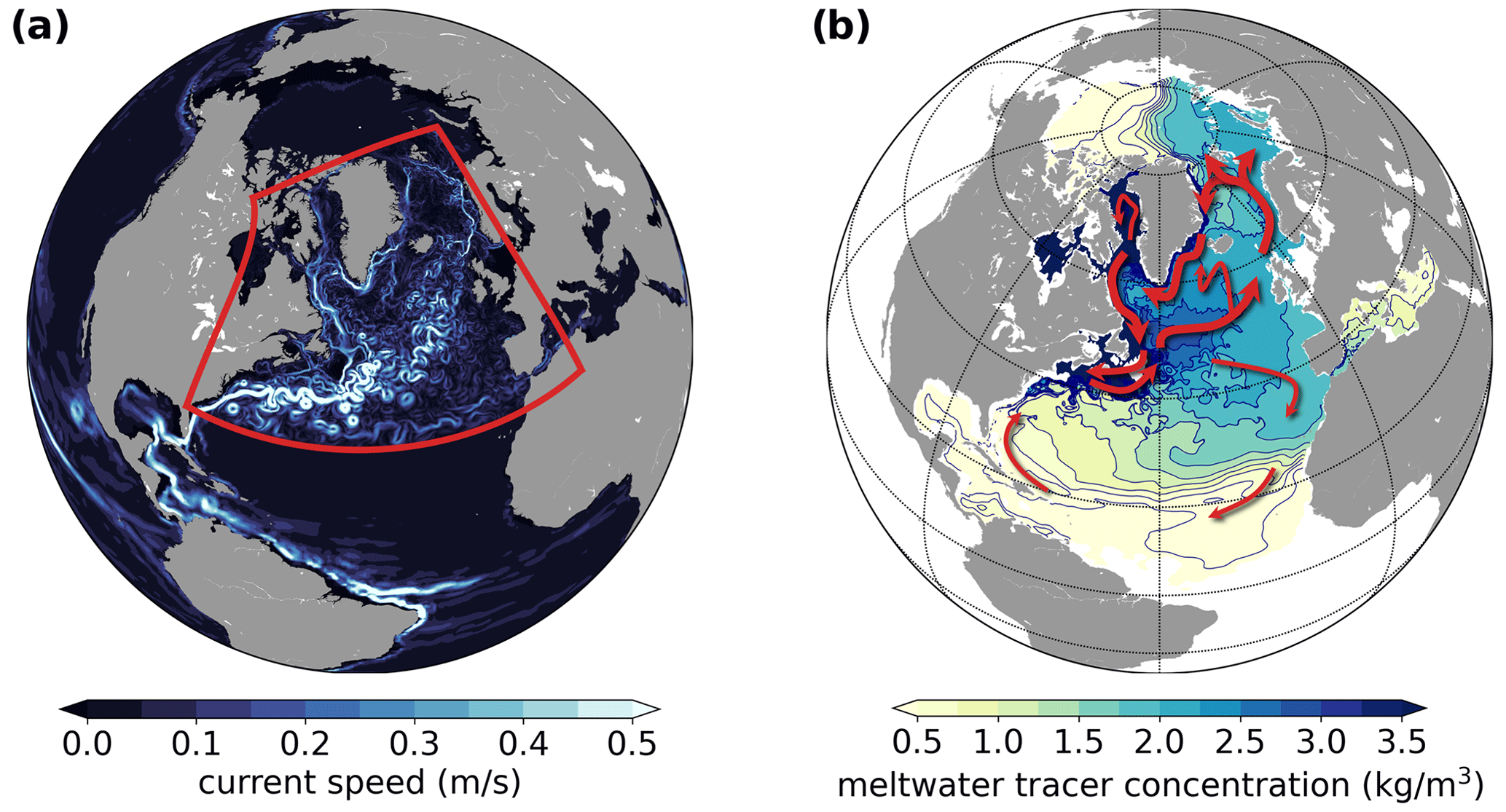
Figure 1 (a) Snapshot (5 d mean) of upper-ocean current speed at about 100 m depth, exemplifying the impact of the grid refinement. The area covered by the two-way nested model VIKING10, in which the grid is refined from $\mathrm{1}/\mathrm{2}$ to $\mathrm{1}/\mathrm{10}$^∘, is marked by the red frame. (b) Concentration of the passive tracer tagging the freshwater perturbation (enhanced Greenland runoff) at the end of the experiment after 100 years (same 5 d mean, also at 100 m depth). Red arrows sketch the main pathways of the freshwater added.

Table 1 Overview of numerical experiments: coupled experiments apply the ECHAM6 atmosphere model, forced ones use CORE-II atmosphere reanalysis. In the $\mathrm{1}/\mathrm{2}$^∘ global ocean model, eddies are parameterized using GM (Gent and McWilliams, 1990), whereas in the North Atlantic nest with a grid resolution of $\mathrm{1}/\mathrm{10}$^∘, mesoscale eddies are simulated explicitly instead. A freshwater flux (FWF) of 0.05 Sv is added as seasonally varying runoff using a spatially heterogeneous but time-invariant pattern along Greenland's coasts in the perturbation experiments. See main text for details.

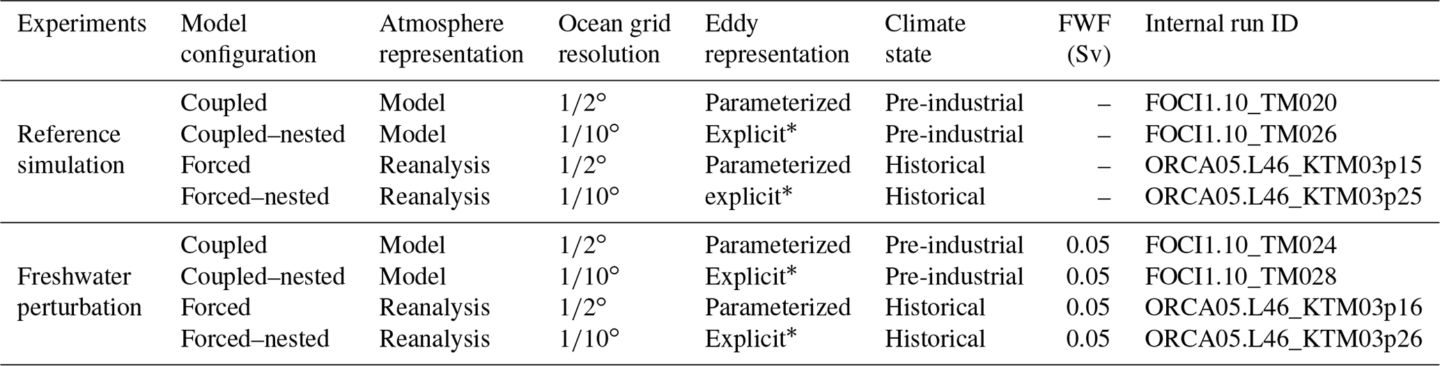
^* Note: GM is also applied to the global host model of the nested configurations.

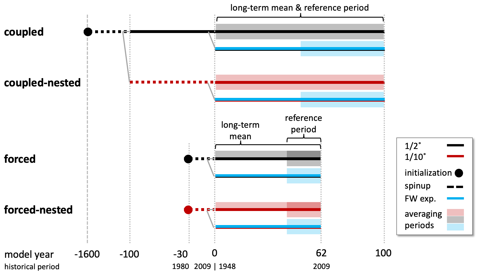
Figure 2 Sketch of the experiment setup showing the spinup, branching off, and duration of all model simulations. All simulations were initialized using the PHC3.0 ocean climatology (Steele et al., 2001), starting from rest. Coupled non-eddying and eddying experiments share the same low-resolution 1500-year-long spinup; coupled freshwater experiments were branched off of the respective control run after 10 years. See main text for details.

2 Model configurations and experiment

The Flexible Ocean and Climate Infrastructure (FOCI) at GEOMAR (Matthes et al., 2020) combines the ECHAM6.3 atmosphere (Stevens et al., 2013; Müller et al., 2018) and the JSBACH land models (Reick et al., 2013) with the NEMO3.6 ocean (Madec, 2016) and LIM2 sea-ice models (Fichefet and Maqueda, 1997) using the coupler OASIS3-MCT (Valcke, 2013). Atmosphere (and land) components are applied to a T63 (1.9^∘) grid with 95 vertical levels reaching up to 0.01 hPa. Ocean (and sea-ice) models run on the ORCA05 grid ($\mathrm{1}/\mathrm{2}$^∘) with 46 vertical levels resolving the top 100 m of the water column at 6–20 m and using partial cells at the bottom. The coupled FOCI simulations presented here all branch off from a 1500-year-long pre-industrial control run (internal ID FOCI1.3-SW038), which was started with an atmosphere and ocean at rest and initialized using ocean potential temperature and salinity fields of the PHC3.0 climatology (Steele et al., 2001). Further details of FOCI and the pre-industrial climate control experiments are found in Matthes et al. (2020).

FOCI was specifically designed for applying two-way high-resolution regional nesting to the ocean component of a coupled climate model using adaptive grid refinement in Fortran (AGRIF; Debreu et al., 2008). For the VIKING10 nest used here and first introduced in Matthes et al. (2020), the grid refinement is applied to 30–85^∘ N in the Atlantic to study subpolar processes and to include the entire coastline of Greenland for the freshwater-release experiment described below (Fig. 1a). The nest features a 5-times-finer horizontal grid resolution of $\mathrm{1}/\mathrm{10}$^∘ and hence simulates a strongly eddying ocean, i.e., resolves the Rossby radius, in large parts of the refinement region. Since the ORCA05 tripolar grid is stretched towards the North Pole, the resolution around Greenland of 24–32 km at $\mathrm{1}/\mathrm{2}$^∘ reaches 4.5–6.5 km with the refinement to $\mathrm{1}/\mathrm{10}$^∘ applied. Still, this must be considered only eddy-permitting poleward of about 50^∘ latitude (Smith et al., 2000; Hallberg, 2013). Eddy formation along the southwestern coast of Greenland is enhanced by applying no-slip boundary conditions in the nest model near Cape Desolation; free slip is used otherwise. With a default $\mathrm{1}/\mathrm{2}$^∘ ocean grid spacing, the standard FOCI ocean clearly is non-eddying, and the effect of mesoscale eddies is parameterized following Gent and McWilliams (1990), applying a space-invariant eddy-induced velocity coefficient (rn_aeiv_0) of 1000 m² s⁻¹. This also applies to the global $\mathrm{1}/\mathrm{2}$^∘ host model running with the eddying nest. The benefit of resolving mesoscale ocean fronts with the nested configuration for air–sea fluxes is limited because the exchange fluxes are computed by the atmosphere model on its coarser grid. Larger-scale improvements in surface conditions due to the more realistic ocean dynamics do imprint on the coupled system. For details of the coupling approach with two-way nesting, please see Matthes et al. (2020).

Using the same ocean and sea-ice model, we run ocean-only simulations without and with the VIKING10 nest using CORE-II atmospheric forcing (Large and Yeager, 2009). These hindcast experiments cover the historical period 1948–2009; i.e., they extend over 62 years. The initial state of these simulations, both without and with nest, is generated by initializing the model with the PHC3.0 climatology (Steele et al., 2001) and running a 30-year spinup from 1980 to 2009. Parameter settings are the same as for the coupled-model configurations, with the exception of applying a weak sea-surface salinity restoring towards the PHC3.0 climatology in the open ocean (rn_deds $=-\mathrm{33.33}$ mm d⁻¹, i.e., 180 d for the model's 6 m thick top layer, and rn_sssr_ds = 0.5 additionally limits the associated salinity change) being added to the surface freshwater flux (see Behrens et al., 2013; Danabasoglu et al., 2014).

In the following, we refer to simulations with interactive atmosphere as “coupled”, ocean-only experiments as “forced”, and simulations including the VIKING10 nest as “nested” (see Table 1 and Fig. 2 for an overview). The latter we also address as “eddying”, whereas the standard setup without nest is “non-eddying”. For the analysis and results presented in the following, it is important to understand that model parameters were optimized for the coupled simulations with FOCI and that parameters used for the nested configuration FOCI-VIKING10 are only scaled proportionally according to (non-linear) dependencies on grid resolution and time stepping, which mostly affects viscosity and diffusion settings. The ocean-only experiments were simply executed with the same set of parameters as their coupled counterpart – no further “tuning” was undertaken. Coupled and forced simulations differ in their climate state, as all FOCI simulations are run under pre-industrial boundary conditions, whereas the ocean-only simulations are forced with “historical” atmospheric conditions.

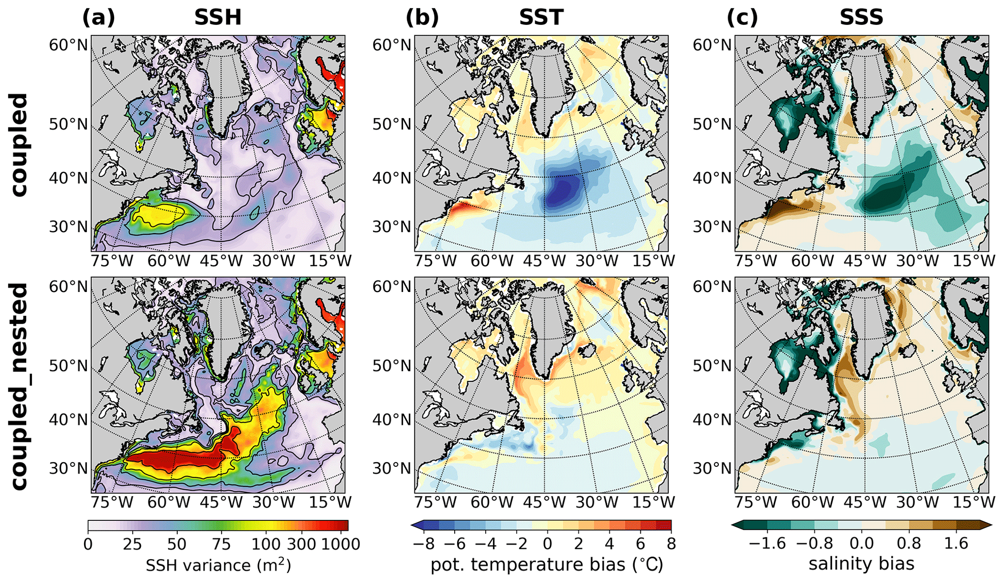
Figure 3 Examples of improvements by the regional-grid refinement from $\mathrm{1}/\mathrm{2}$^∘ (coupled) to $\mathrm{1}/\mathrm{10}$^∘ (coupled–nested): (a) enhanced mesoscale activity indicated by sea-surface-height (SSH) variance in 5 d mean output, (b) reduced North Atlantic cold bias in sea-surface temperature (SST), and (c) improved representation of sea-surface salinity (SSS). All examples from the coupled-model experiments FOCI and FOCI-VIKING10 based on 50-year means. The SST and SSS biases are computed as difference from HadISST (Rayner, 2003), mean over 1870–1899 to compare with pre-industrial model experiments, and WOA98 climatological salinity (Levitus et al., 1998), respectively.

The eddying simulations feature pronounced boundary currents and a meandering North Atlantic Current (NAC) – see Fig. 1a. As a result of the improved dynamics, strength and shape of the subpolar gyre are well represented, and the NAC follows a less zonal, more realistic path forming the so-called Northwest Corner (Lazier, 1994) and a northward and then eastward turning of the currents off Newfoundland and the Flemish Cap. This is shown by the standard deviation in sea-surface-height anomalies computed from the 5-daily-mean model output of a 50-year reference period (Fig. 3a). The realistic simulation of the NAC path nearly eliminates the cold bias, a mismatch of simulated and observed sea-surface temperature (SST) in the mid-latitude North Atlantic, which is a prominent feature of the non-eddying simulations (Fig. 3b). Less often referred to, the cold bias is associated with a fresh bias, a salinity low of up to 2, equally caused by an overestimated southeastward spreading of polar waters in non-eddying simulations (Fig. 3c). The eddying simulations have saltier overflow water and hence tend towards saltier conditions in the Labrador and Irminger seas, which yields more intense, sometimes overly strong deep convection in winter, as is discussed in the next section. All of these features concur with earlier studies comparing NEMO-based simulations of similar-resolution spread (Treguier et al., 2005; Talandier et al., 2014; Marzocchi et al., 2015; Hewitt et al., 2020; Koenigk et al., 2021)

The freshwater-release experiment presented is simplified in the overall magnitude, as well as in its step-like spontaneous onset of the perturbation, but it is realistic in the spatial distribution and seasonality of the additional freshwater flux inserted along the coast of Greenland. The perturbation is constructed from the monthly mean runoff plus discharge fluxes of Bamber et al. (2018) by averaging the period 1992–2016, which includes better mass balance estimates and covers the pattern of recently increased GrIS melting. Spatial heterogeneity and the seasonal cycle of the original data are maintained. Data from glaciers outside of Greenland are not considered. The resulting climatology is then scaled to a moderate but significant perturbation of 0.05 Sv on the annual mean (see Martin et al., 2022, their Fig. S1). This flux is released as an interannually invariant liquid runoff along Greenland's coast over 62 and 100 years in the forced and coupled experiments, respectively, in addition to the simulated (coupled) or prescribed runoff (forced). We note that this perturbation yields a barystatic sea-level rise of 0.44 m over 100 years (Martin et al., 2022), which is about 5 times the magnitude projected by simulations under the RCP8.5 climate scenario (Goelzer et al., 2020).

We are aware that the way we prescribe the freshwater perturbation is a simplification: applied to the ocean surface layer, maximum runoff in June to August, and all liquid runoff. In reality, half of the mass loss of Greenland's glaciers is dynamical discharge (The IMBIE Team, 2020), such as iceberg calving, though surface melting has made the bigger (approximately two-thirds) contribution in recent years (Enderlin et al., 2014). Further, meltwater runoff is first entrained into the fjord circulation, which causes both a vertical redistribution and a temporal delay of several weeks before entering the open ocean (Straneo and Cenedese, 2015; Straneo et al., 2016). However, we consider associated errors to be small for three reasons: firstly, it is estimated that about half of all icebergs already melt inside the fjords (Enderlin et al., 2016); secondly, Marson et al. (2021) have not found a major impact on deep convection by explicitly simulating icebergs; and thirdly, we find that the ocean model effectively distributes the prescribed freshwater over depth on the Greenland shelf, whereby a delay or accumulation arises so that the seasonal peak in freshwater content on the shelf is shifted by about a month compared to the prescribed perturbation.

We trace the distribution pathways of the added freshwater by applying a passive tracer. The related model output provides tracer concentration in kg m⁻³. This means that, at any given time, the global tracer mass computed as the global sum of the product of tracer concentration and grid-cell volume equals the accumulated freshwater perturbation added as runoff from Greenland. Using the passive-tracer concentrations, we compute an error of < 1 % and ≤ 5 % after 62 years for the non-nested and nested configurations, respectively, due to the not entirely conservative nature of the NEMO tracer and AGRIF codes for the given setup (e.g., linear free surface). The tracer proves to be a powerful tool to visualize and understand the pathways of Greenland meltwater redistribution in the ocean, as demonstrated in Fig. 1b.

3 Results

We compute the response to the freshwater perturbation as a deviation of the experiment from the reference simulation (perturbation minus control run). As such, the difference is affected by differences in internal variability between the simulations. Internal variability is more pronounced in the coupled experiments, whose atmosphere evolves freely under pre-industrial forcing, whereas the forced experiments are bound by the historical atmospheric conditions. Further, mesoscale dynamics simulated explicitly in the eddying experiments enhance ocean internal variability. Lastly, the perturbation experiments all have a certain adjustment period, and a new quasi-equilibrium state, especially for the AMOC, can only be expected to exist after several decades (e.g., Swingedouw et al., 2013; Jackson and Wood, 2018). Considering all this (see Appendix A for details), we found optimal signal-to-noise ratios by using the averaging periods illustrated in Fig. 2. In the coupled case, we compute the reference mean state over years 1–100 and the perturbed state from the period 51–100. For the forced experiments, noise can be optimally reduced by averaging over the same years 43–62 for the reference and perturbed states. To present the control long-term mean state of each model configuration, we use years 1–100 and 1–62 for the coupled and forced simulations, respectively. These periods are used throughout this study unless stated otherwise.

We present our results structured by quantities and processes rather than discussing the reference states first and then the responses. This is to highlight the role of the respective mean state in the consequences of the freshwater perturbation.

Table 2 AMOC mean state and response to freshwater perturbation measured by the maximum transport in the overturning streamfunction computed from zonally averaged Atlantic basin meridional velocities. Mean state and response are computed over years 1–100 (1–62) and 51–100 (43–62) for coupled (forced) experiments, respectively. Additionally, responses for the two coupled experiments computed as average over years 43–62 are provided in square brackets. The standard deviation σ based on monthly mean model output is provided as a measure of internal variability and noise in the signal of the response. Correlation coefficients (Pearson's r) between annual-mean AMOC strength and Denmark Strait (DS) overflow potential density (p_ref=0) as well as March-mean mixed-layer depths (MLDs) in the Labrador Sea after applying a decadal boxcar averaging filter to all time series are listed. Correlations are computed from the reference experiment over 100 and 62 years for the coupled and forced configurations, respectively, applying an 11-year rolling mean to highlight a linkage on decadal and longer timescales. All values are given in sverdrup (1 Sv =10⁶ m³ s⁻¹), except for the correlation coefficients in the last two columns.

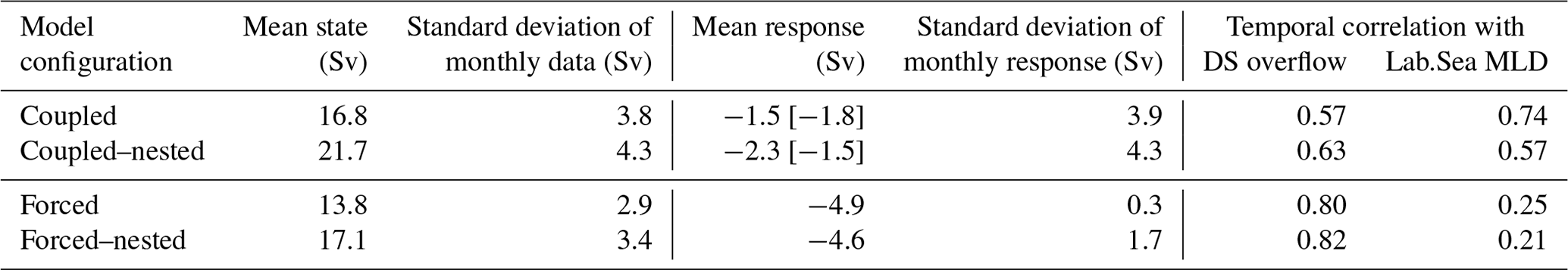
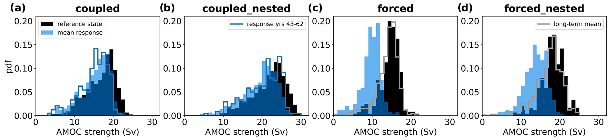
Figure 4 Statistical distribution of monthly mean AMOC maximum strength (Sv) in model reference states (black bars) and perturbed states (blue bars, transparent). Blue outlines in panels (a) and (b) show response distribution for years 43–62, and light gray lines in panels (c) and (d) depict the distribution of the long-term mean period (years 1–62).

3.1 Ocean mean states and responses

AMOC

The strength of the AMOC can be considered a diagnostic integrating all the effects triggered by the additional freshwater input into the SPNA, since the overturning is sensitive to changes in temperature, salinity, surface heat flux, and deep mixing in this region, all of which will be addressed in the following. We summarize the AMOC mean states and changes in response to the freshwater perturbation of the four configurations in Table 2 and present the associated monthly to interannual variability in Fig. 4. AMOC strength is defined here as the maximum of the Atlantic streamfunction in latitude–depth space computed from the zonally averaged meridional velocity of monthly mean model output.

The weakest AMOC is simulated by the non-eddying forced configuration at 13.8 Sv; with 21.7 Sv, the coupled–nested setup features the strongest overturning (see Table 2). Coupled and forced–nested experiments are relatively close at 16.8 and 17.1 Sv. For comparison, the observed strength of the AMOC at 26.5^∘ N is about 17–18 Sv, with a standard deviation of 3.4 Sv in monthly data (McCarthy et al., 2015; Biastoch et al., 2021). In both the coupled–nested and the forced–nested configurations, the explicit simulation of mesoscale eddies increases the magnitude and internal variability of the AMOC, which agrees well with similar comparisons (Hirschi et al., 2020; Biastoch et al., 2021). Furthermore, the coupled configurations simulate a stronger AMOC than their forced counterparts, which could be related either to coupling with an interactive atmosphere, as in Hirschi et al. (2020), or to the different climate mean states, historical (forced) and pre-industrial (coupled).

Variability is measured as monthly standard deviation of the maximum strength (Table 2), and the eddy-related increase amounts to 0.5 Sv in the coupled and the forced configuration. However, the interactive coupling with the atmosphere adds more noise, and AMOC variability is enhanced by about 1 Sv in the coupled setups compared to the respective forced ones. This is well depicted by the histograms of AMOC mean states in Fig. 4 (black bars).

In response to the freshwater perturbation, we expect the AMOC to weaken, which is simulated by all four model configurations. This is depicted by the blue histograms in Fig. 4. The magnitude of the reduction in maximum overturning strength varies considerably. We find the two forced configurations to be more sensitive, simulating declines of 4.9 and 4.6 Sv (36 % and 27 %), with the overall weakest AMOC being most vulnerable. The coupled configurations simulate reductions of 1.5 to 2.3 Sv (9 % and 11 %). These longer simulations also show that internal variability matters, and thus, a 50-year period is used to compute the response. For comparison, decadal averages of AMOC weakening in these last 50 years of the perturbed run (i.e., five independent samples) range from 1.0 to 1.9 Sv for the coupled and vary within 1.1–3.0 Sv for the coupled–nested experiment.

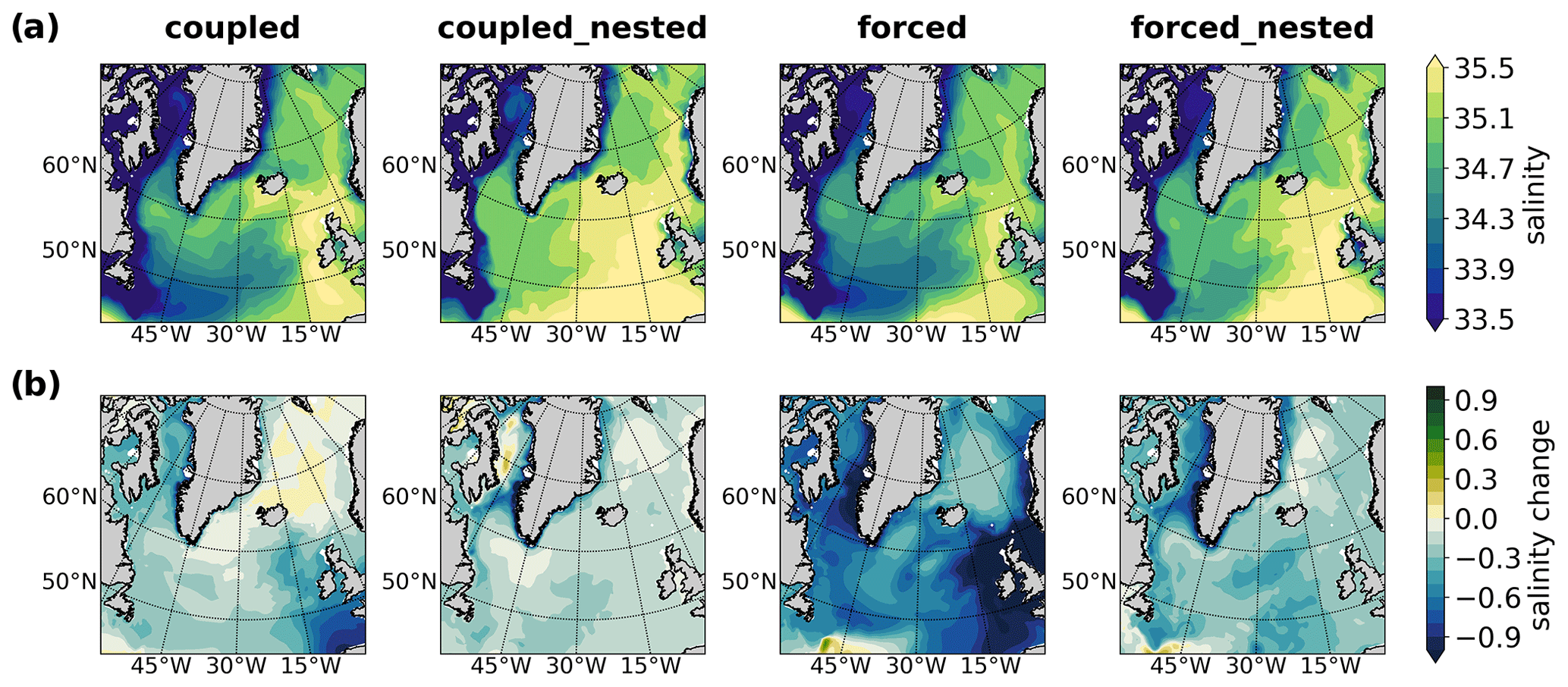
Figure 5 (a) Long-term mean state of upper-ocean (0–200 m) annual-mean salinity and (b) the change due to the freshwater perturbation. The response is computed as the difference in the means over years 51–100 and 43–62 in the coupled and forced cases, respectively.

Large-scale upper-ocean salinity and freshening

The additional freshwater released from Greenland enters the East and West Greenland Currents (EGC and WGC) and is transported south with the Labrador Current (Fig. 1b). Reaching Newfoundland, or rather the so-called Northwest Corner, we find major deviations in the freshening patterns (Fig. 5). Lack of mesoscale dynamics (being parameterized instead) and a resulting too-zonal positioning of the NAC lead to a massive, NAC-focused advection of freshwater across the Atlantic in the non-eddying simulations. In contrast, the eddying simulations, which simulate narrower, stronger boundary currents and a more realistic Gulf Stream separation and Northwest Corner dynamics (see Figs. 1 and 3), accumulate freshwater along the American coast down to the Mid-Atlantic Bight. In these simulations, explicitly resolved eddies then entrain the freshwater into the Gulf Stream extension and NAC, which is further discussed in Sect. 3.2. The described redistribution pathways agree with earlier tracer simulations by Dukhovskoy et al. (2016) and Böning et al. (2016).

The explicitly simulated eddies and stronger meandering cause a much wider spreading of the freshwater across the SPNA than achieved by the eddy parameterization in the coarse-resolution models, which are limited by their biased mean flow. This is expressed in the change in upper-ocean salinity, here averaged over the top 200 m, in response to the freshwater perturbation (Fig. 5b). While all four configurations yield an overall freshening of the SPNA, the upper-ocean freshening is stronger in the two non-eddying simulations – including a significant intensification towards the east – than in the eddying counterparts.

Similarly prominent is the stronger freshening in the forced experiments compared to the coupled counterparts. This is an indirect effect in consequence of the greater weakening of the AMOC in these simulations compared to the coupled ones, as shown above. The reduced AMOC means less northward advection of saline and warm subtropical waters (see, e.g., Smeed et al., 2018). As detailed by Griffies et al. (2009) and discussed further below, forced model configurations are prone to an overly strong positive salinity feedback. A visible secondary process causing local upper-ocean freshening along the northern rim of the Labrador Sea is a southward advancement of the marginal sea-ice zone leading to decreased evaporation, as well as to southward-shifted melting of sea ice in all but the coupled experiment.

Figure 6 (a) Long-term mean state of upper-ocean (0–200 m) annual-mean potential temperature and (b) the change in consequence of the freshwater perturbation. The response is computed as the difference in the means over years 51–100 and 43–62 in the coupled and forced cases, respectively.

Figure 7 (a) Long-term mean state of annual-mean mixed-layer depth and (b) the change in consequence of the freshwater perturbation. The response is computed as the difference in the means over years 51–100 and 43–62 in the coupled and forced cases, respectively. Sea-ice coverage (ice concentration > 15 %) in the reference state is indicated by white areas with hatching, and sea-ice expansion in the perturbed state is bright blue.

Large-scale upper-ocean temperature and cooling

As a consequence of a weaker AMOC, the upper SPNA experiences widespread cooling. Averaging over the top 200 m and all seasons, this cooling can reach 2.1–2.3 ^∘C in some areas (Fig. 6). SST exhibits an even larger decline by 3.1–4.5 ^∘C, especially in mid-winter (February or March), where cooling occurs in the Labrador Sea due to reduced deep-convection activity and more extensive sea-ice coverage. This is except for the coupled experiment with the smallest AMOC decline, in which annual-mean cooling is limited to < 1.3 ^∘C. All experiments also exhibit pronounced cooling in the eastern SPNA, which is as strong as – and in coupled, even stronger than – the temperature decline in the northern Labrador Sea. This eastern cooling is carried by the Irminger Current from the eastern North Atlantic (ENA) into the Irminger Sea.

The response is different and quite diverse for the Nordic Seas. We observe a warming of up to 2.3 ^∘C in the top 200 m in the coupled experiment but only < 1 ^∘C in all other cases. The relatively strong warming in the coupled experiment is caused by an overall weaker advection of the freshwater perturbation into the Nordic Seas (Fig. 5b) so that the mixed layer is slightly deepening across the Nordic Seas (Fig. 7). The warming extends to 1000 m and is associated with a slight increase of around 50 m in the overturning north of the overflows, which is in agreement with the findings of Stouffer et al. (2006) for similar models. In contrast, the Nordic Seas warming in the forced non-eddying experiment is limited to the recirculation path of the Atlantic water and is associated with a considerable shoaling of the mixed layer by 100–150 m along this path.

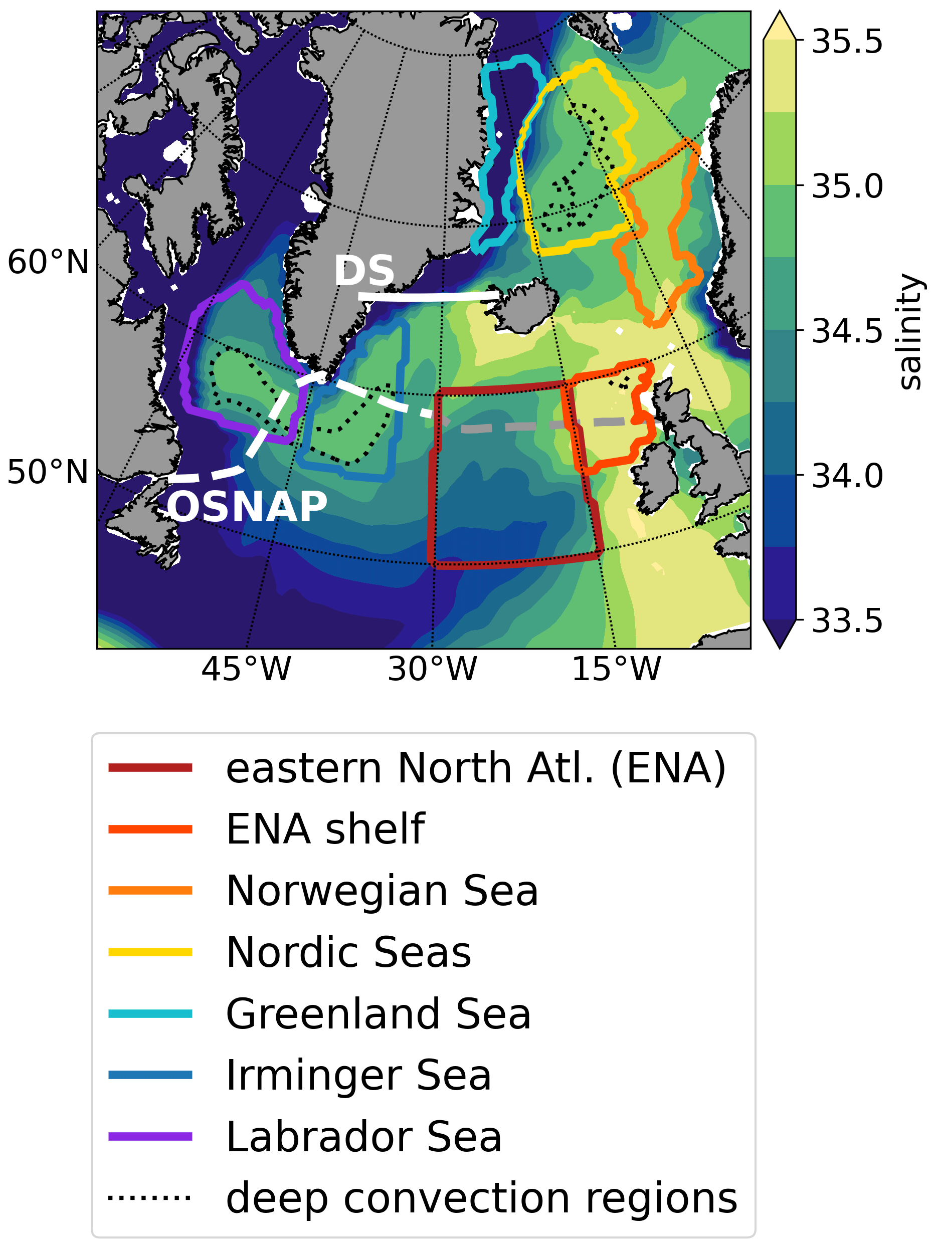
Figure 8 Map of regions selected for computing water properties and mixed-layer statistics. All regions are defined by geographic coordinates. Shelf regions are excluded by prescribing a minimum depth of 1500 m for the Nordic, Irminger, and Labrador seas and of 1000 m for the Norwegian Sea. The ENA shelf region excludes areas shallower than 100 m. In contrast, the Greenland Sea region is defined for areas shallower than 500 m. White lines indicate the Denmark Strait (DS, solid) and Overturning in the Subpolar North Atlantic Program (OSNAP, Lozier et al., 2019) (dashed) cross-sections. For reference, the long-term mean salinity of the coupled simulation averaged over the top 200 m is shown (cf. Fig. 5a) along with the March-mean 500 m mixed-layer depth contour because these quantities guided the region selection.

Water mass transformation

For the illustration of the different water masses and their transformation in the four model configurations, as well as their property changes under the freshwater perturbation, we define a number of regions following the path of the Atlantic water to the deep-convection sites in the SPNA and Nordic Seas. Further, we confine the volume-weighted averages of potential temperature and salinity to the top 200 m. In addition, we provide these properties from the overflow depth at the Denmark Strait (DS). The regions of interest are depicted in Fig. 8, with the color coding associated with the warm northward inflow on the eastern side (red–orange–yellow colors) and cold southward flow of polar water (cyan) and deep-convection regions in the west (blue and purple colors). This color coding is used in subsequent plots of Figs. 9 and 11. The ENA is defined as the region between 15–30^∘ W and 50–60^∘ N, following Koul et al. (2020) and Holliday et al. (2020).

Focusing first on the mean states and beginning in the ENA (dark-red-filled circles), our simplified diagrams of temperature vs. salinity (TS) clearly illustrate the strong fresh bias present in the mean state of the two non-eddying simulations due to the misrepresentation of the NAC, in which ENA salinity is 0.8–0.9 lower than in the two nested, eddying simulations (Fig. 9; cf. Fig. 3c). Interestingly, taking the average just east of the ENA region, towards the European shelf (here referred to as ENA shelf, bright red), the salinity deviations are much smaller, within 0.1. In particular, in the coupled–nested configuration, properties in ENA and ENA shelf are almost identical. It is this TS characteristic that sets the baseline for the water mass transformation in the SPNA and Nordic Seas (Lozier et al., 2019). With 10–11 ^∘C, the potential temperature is very similar for all model configurations, except for the coupled, non-eddying one, in which the ENA region is strongly influenced by the cold bias with respect to late 19th-century reanalysis (see Fig. 3b). The forced experiments must thus be considered relatively cool running with historical atmospheric forcing but having a weaker AMOC and hence less northward heat transport. The TS diagram illustrates the transition of the Atlantic water by freshening and predominantly cooling along its path from the ENA region (red) to the Nordic Seas (yellow) and ultimately imprinting its characteristic onto the overflow water at the Denmark Strait (DS, black). The latter is about 2 ^∘C warmer in the eddying than in the non-eddying runs, likely due to more vigorous deep convection (deeper maximum mixed-layer depths, not shown).

The relatively fresh and cold polar water (cyan circles) exported from the Arctic Ocean and advected south in the EGC interacts with waters of the Irminger Current, carrying properties of the ENA and ENA shelf regions. We find upper-ocean properties of the Irminger (blue) and Labrador seas (purple) situated roughly halfway between these two source waters. The interior Labrador Sea has a tendency to be slightly cooler and/or fresher than the Irminger Sea. In both regions, the coupled reference simulations are a little saltier than their forced counterparts, and the same holds for the comparison between eddying and respective non-eddying simulations. We suggest a lack of offshore Ekman transport in the coupled configurations and generally stronger deep convection in the nested ones as causes, and we discuss these further below. Another more obvious salinity and thus density difference is found between the boundary current (small purple circles) and the interior Labrador Sea (purple). This difference is significantly smaller in the non-eddying than in the respective eddying simulations and can be related to an insufficient exchange across the shelf break in the latter (more details in Sect. 3.2).

The freshwater perturbation leads to a freshening and cooling in the ENA and ENA shelf regions in all configurations (compare crosses “+” with filled circles). The response is larger in the forced configurations than in the coupled ones and larger in the non-eddying than in the respective eddying simulations. In the forced experiment, this leads to a density decrease of 0.4 kg m⁻³, whereas in the coupled–nested one, the density change is minor. The freshening effect by the perturbation weakens as the Atlantic water progresses into the Nordic Seas.

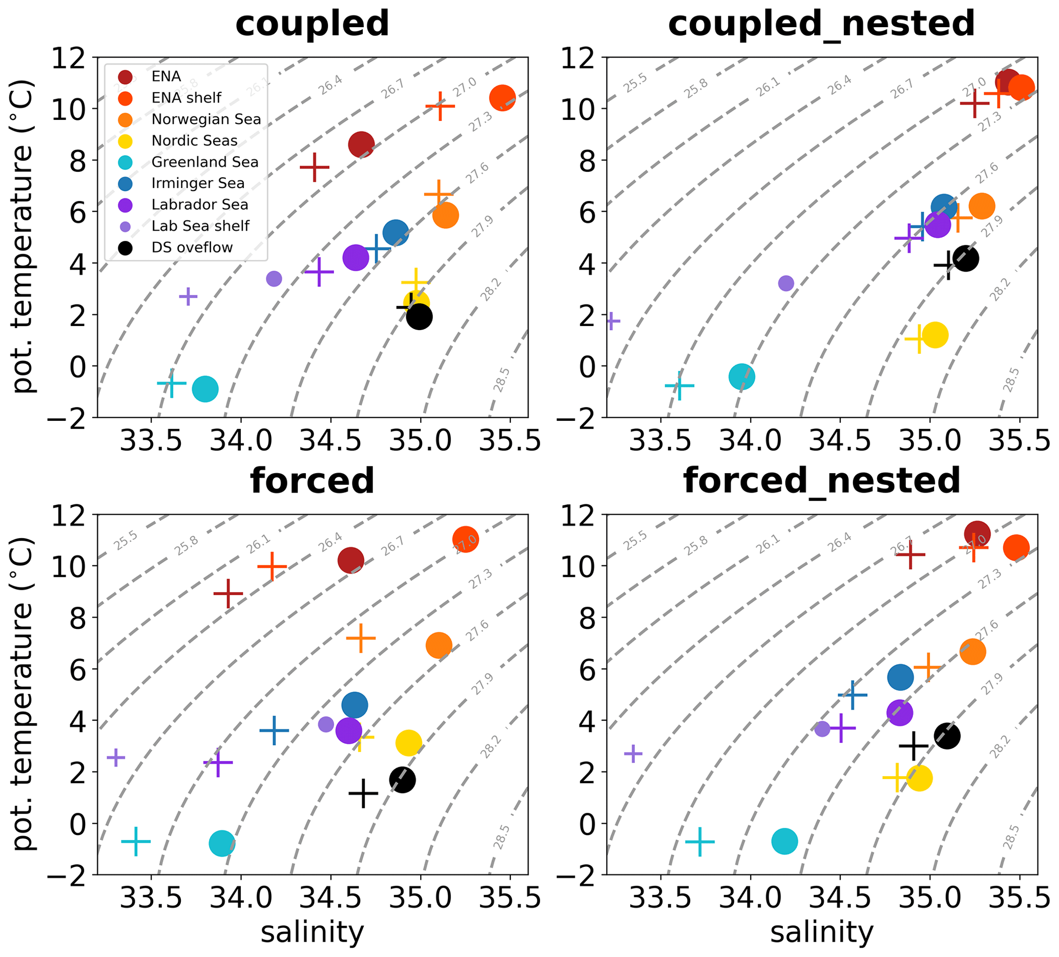
Figure 9 Mean water properties of regions depicted in Fig. 8 (same color coding) from the reference simulation (filled circles) and the perturbation experiment (“plus” symbols). Symbols depict properties averaged over the upper 200 m, except for the Denmark Strait (DS) overflow (in black) where values from the deepest grid cells (approx. 600 m depth) along the section at about 65.7^∘ N are averaged. For the Labrador Sea region (purple), properties on the continental shelf (smaller symbols) are shown in addition to the ones from the interior part (regular-sized symbols). The shelf is defined as areas shallower than 500 m in the region 62–46^∘ W and 56–65^∘ N, i.e., within the same geographical box as the deep, interior Labrador Sea (purple frame in Fig. 8).

With respect to the AMOC weakening discussed above, we stress that the density of the Denmark Strait overflow hardly changes in the perturbed coupled experiments. There occurs, however, a significant density decrease by 0.1–0.15 kg m⁻³ in the two forced experiments. The latter two happen to be the model configurations with the overall stronger AMOC decline, which we suggest is related to the change in overflow properties. This is supported by a strong correlation on decadal timescales between AMOC strength and DS overflow density (∼ 0.8). The correlation with Labrador Sea winter mixed-layer depth is much weaker (∼ 0.23; see Table 2), which agrees well with the results of Behrens et al. (2013) and Biastoch et al. (2021).

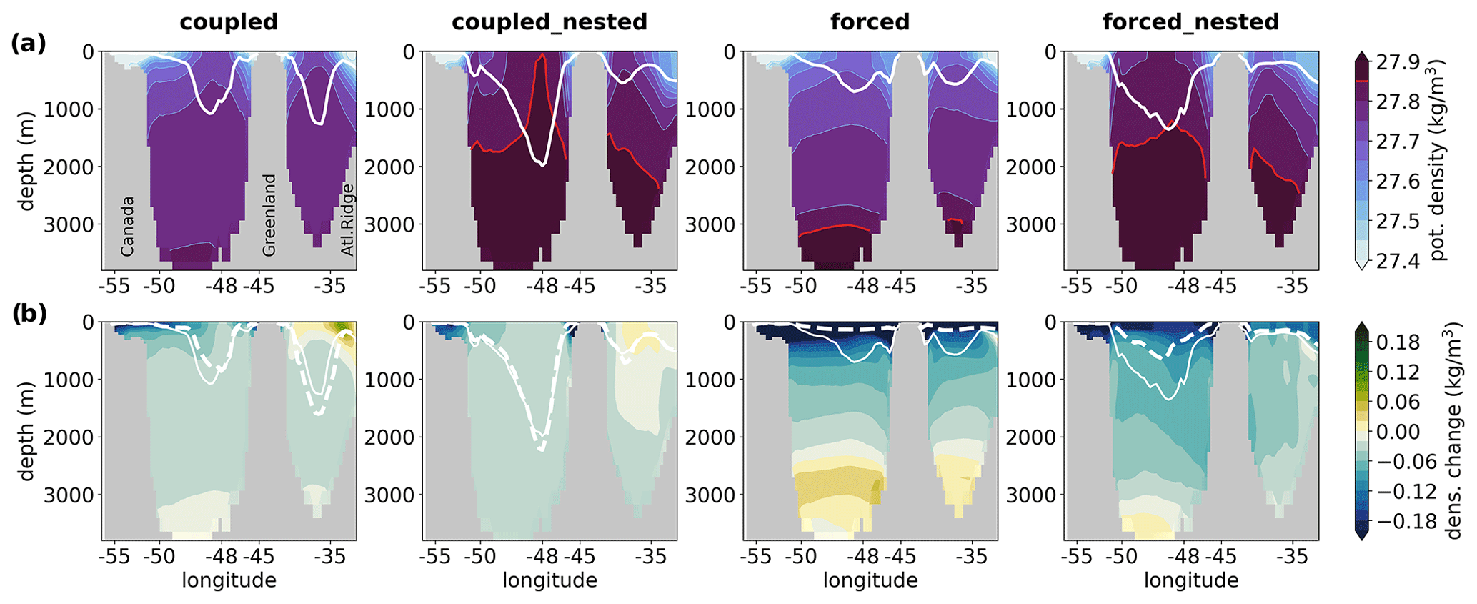
Figure 10 Cross-section through Labrador and Irminger seas showing (a) March-mean potential density (σ₀) and (b) the change due to the freshwater perturbation. The solid and dashed white lines depict the March-mean mixed-layer depth of the reference and perturbed states, respectively. The red contour in panel (a) highlights densities > 27.85 kg m⁻³. The cross-section follows the location of the OSNAP line (see Fig. 8).

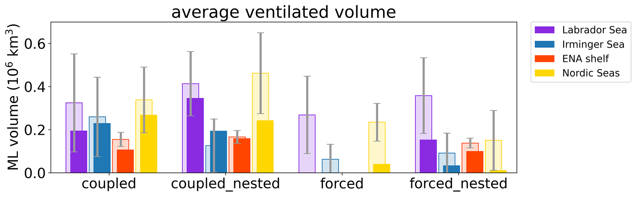
Figure 11 March-mean ventilated water volume for the reference state (pale bars in background) and perturbation experiment (in foreground) for regions with deep convection. Ventilated volume is computed as mixed-layer depth (MLD) times grid-cell area, where MLD > 500 m. Gray error bars indicate ± 1 standard deviation of interannual variability.

The density structure of cross-sections along the Overturning in the Subpolar North Atlantic Program (OSNAP) line (Lozier et al., 2019) through the Labrador and Irminger seas presented in Fig. 10 differs considerably between model configurations and has implications for the response to the freshwater perturbation. The water mass in the interior Labrador and Irminger seas is denser in the two eddying configurations than in the non-eddying ones. The forced non-eddying configuration exhibits a stronger vertical density gradient than its coupled counterpart. This is likely a consequence of the shallower mixed layer in the forced configuration (Fig. 7), as well as of the much shorter spinup (30 years) compared to the coupled experiment (1500 years). Therefore, properties of the initialization fields are still visible in the deep ocean of the forced run. The forced non-eddying experiment also features the smallest ventilated volume in the Labrador and Irminger seas (Fig. 11, purple and blue bars). We define ventilated volume as mixed-later depth (MLD) times grid-cell area where MLD exceeds 500 m to focus on deep overturning. The larger the ventilated volume, the closer dense overflow waters rise to a mid-depth of about 1000 m. Here, overflow waters are identified by a density of σ₀> 27.85 kg m⁻³ (red contour in Fig. 10a), having been diluted along the way from ≥ 27.9 kg m⁻³ at the Denmark Strait (black circles in Fig. 9). In particular the eddying configurations feature large volumes of overflow water in the deep Labrador and Irminger seas. In contrast, the non-eddying coupled simulation with the densest overflow water at the Denmark Strait shows no water mass identifiable as such in the Labrador and Irminger seas cross-section. Interestingly, this configuration yields the weakest correlation between AMOC strength and DS overflow density (Table 2).

The cross-section in Fig. 10a shows much steeper isopycnal slopes between the boundary currents (light blue) and the interior (dark blue) for the two eddying configurations. As will be further discussed below, this is related to running the ocean model at $\mathrm{1}/\mathrm{2}$^∘ grid resolution with an eddy parameterization but at $\mathrm{1}/\mathrm{10}$^∘ without. However, the higher resolution is not quite sufficient to simulate the full eddy spectrum and hence lacks some mixing between the boundary and interior, which is well parameterized in the non-eddying configuration.

Greenland meltwater enters the boundary currents, enhancing the density gradient to the interior Labrador and Irminger seas. Larger eddies spawned off the WGC due to unique topography around Cape Desolation, and smaller, local ones created by baroclinic instability act to reduce this gradient (Rieck et al., 2019). The magnitude of freshening and the reference mean state of the interior Labrador and Irminger seas are key to understanding the AMOC response. It is the forced non-eddying experiment with the smallest difference between the Labrador Sea shelf and interior water properties (Fig. 9) that presents with a complete loss of ventilated volume for areas of deep convection (MLD > 500 m) under the freshwater perturbation, as shown in Fig. 11. This configuration features the freshest mean state (Fig. 5a) and therefore has the lowest barrier for any additional freshwater carried by the EGC and WGC to enter the deep-convection sites. With deep mixing being shut off, most meltwater stays in the upper subpolar gyre (Fig. 12), reinforcing the response, and less meltwater tracer is found to leave the SPNA with the deep water in this configuration than in any other (Fig. 13, > 1200 m).

In the two coupled configurations, deep-convective mixing is generally more intense (Fig. 11, purple and blue bars), and more heat and salt are brought into the upper ocean . These simulations feature a non-negligible warm (and saline) bias in mid- to deep-ocean layers (Matthes et al., 2020), which may help to maintain the overturning against the freshwater perturbation, and AMOC strength weakens only by 1.5 Sv. We find more meltwater tracers being exported with the deep western boundary current in these configurations, especially in the coupled–nested one (Fig. 13, > 1200 m).

3.2 Mesoscale ocean dynamics

In this section, we discuss the outcome of explicitly simulating mesoscale eddies in the nested configurations instead of parameterizing their effect. We focus on regions and processes of particular relevance for the distribution of Greenland meltwater and its potential impact on deep-water formation. These are exchanged between the boundary current and interior in the Labrador Sea, entrainment into the North Atlantic Current, and leakage into the subtropical gyre.

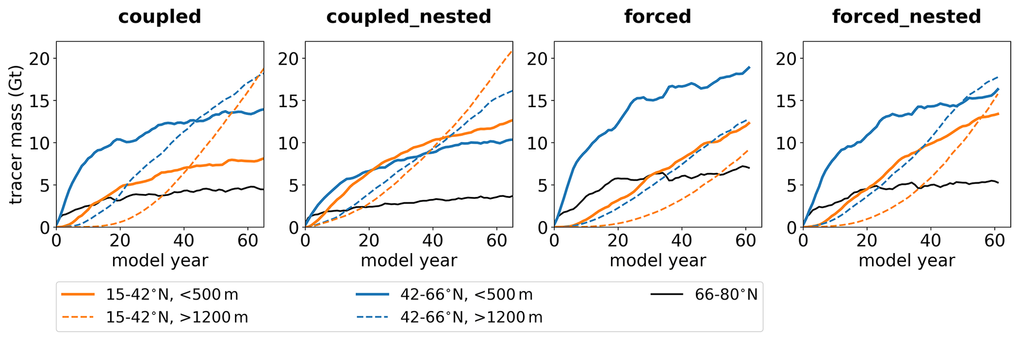
Figure 12 Total meltwater tracer mass for selected regions of the North Atlantic integrated over the entire basin width for the upper 500 m (solid lines) and below 1200 m (dashed lines). Blue lines depict the tracer mass in the subpolar gyre between 42 and 66^∘ N, while orange lines depict the tracer mass in the subtropical gyre (15–42^∘ N). The black lines combine Nordic Seas and Baffin Bay tracer mass inventories, which are approximately of the same magnitude.

Boundary currents

The ocean grid refinement yields realistic dynamics in the nest region (Fig. 1a). We find a strongly eddying ocean where the $\mathrm{1}/\mathrm{10}$^∘ grid sufficiently resolves the Rossby radius, which is the case south of approximately 50^∘ N. In higher latitudes, the finer resolution yields stronger and more focused boundary currents, such as in the Nordic Seas and the Labrador Sea, as well as in the Irminger Sea. For example, the western boundary current transport in the Labrador Sea at 53^∘ N (below 400 m) amounts to 19.4 and 39.3 Sv in the coupled and coupled–nested configurations, respectively, where observations yield an estimate of 30.2 Sv (Zantopp et al., 2017). The grid refinement significantly improves mesoscale variability over large parts of the SPNA (Fig. 3a) but is inadequate to simulate the full dynamical mesoscale spectrum north of 50^∘ N. Nevertheless, we find individual WGC eddies – or Irminger rings – entering the interior northern Labrador Sea (not shown). But smaller mesoscale eddies are crucial for restratification after deep convection in winter (e.g., Rieck et al., 2019) and are not explicitly simulated by the nested configurations. This results in generally steeper isopycnals separating the Labrador Sea shelf from the interior (Fig. 10a). Here, the models parameterizing the cross-frontal transport by eddies show a more realistic hydrography. We suspect that this is an important factor for the stronger deep mixing already in the mean state of the nested simulations (Fig. 11) and for finding less meltwater tracer in the interior Labrador Sea (Fig. 13, 0–200 m). Due to the latter, our results appear contradictory to those of Böning et al. (2016) at first glance, but in fact, they simply suggest that the resolution in our eddying simulations is not high enough to properly simulate the mesoscale in this region, whereas the eddy parameterization in the coarser configurations performs relatively well. This is further discussed in Sect. 4.

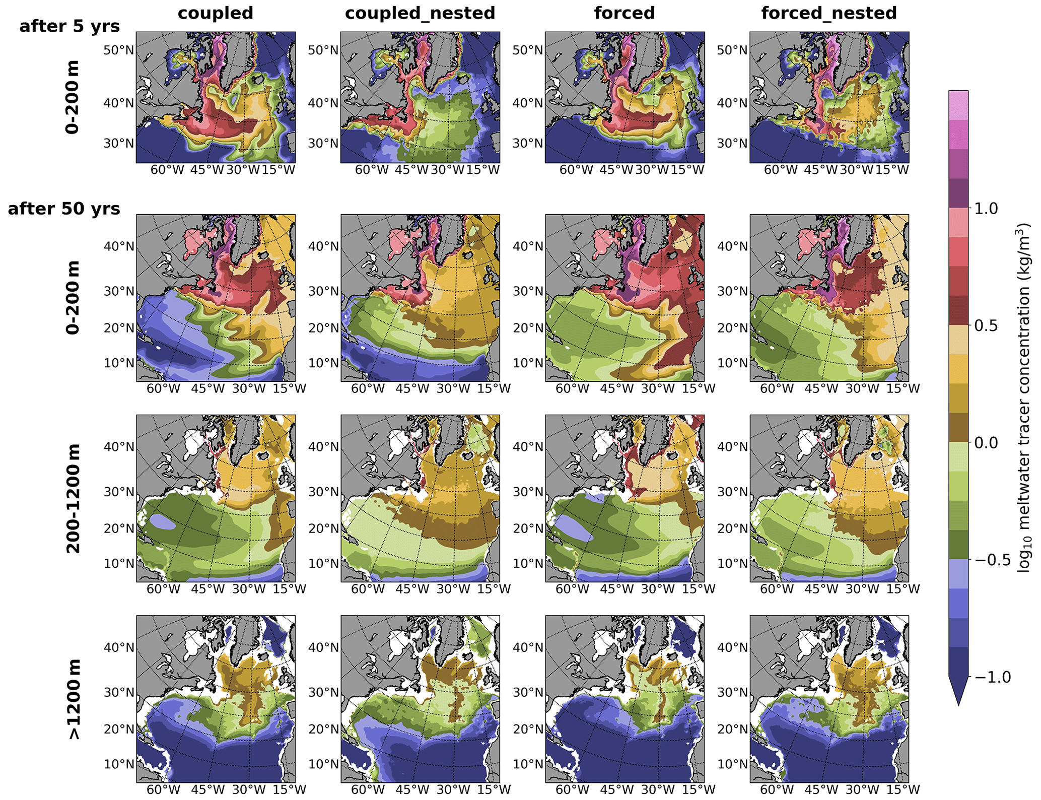
Figure 13 Snapshots (5 d mean) of meltwater passive-tracer concentration 5 years (top row) and 50 years (lower three rows) into the perturbation experiments. For the later period, the average concentration for three depth layers is shown: upper (0–200 m), middle (200–1200 m), and deep ocean (below 1200 m).

The Northwest Corner

The Northwest Corner off Newfoundland is a dynamically active region where the southward-flowing Labrador Current carrying fresh and cold polar waters meets the North Atlantic Current (NAC) transporting warm, salty subtropical water northward. At this switchyard, mesoscale ocean dynamics determine how much polar water – and hence Greenland meltwater – either is mixed into the NAC or continues traveling south into the Mid-Atlantic Bight (Böning et al., 2016; New et al., 2021). Here, we find major divergence between the non-eddying and eddying model configurations. The refined grid of the nest not only significantly mitigates the North Atlantic cold bias (Fig. 3b) but also yields a more realistic, reduced entrainment of Greenland-sourced freshwater into the NAC near the Flemish Cap (Fig. 13, 0–200 m). As in the study of Böning et al. (2016), our eddying configurations transport significantly more meltwater along the coast all the way into the Mid-Atlantic Bight than the non-eddying ones. The eddy parameterization used in the latter prescribes a too-strong entrainment into the NAC, which is illustrated by the upper-ocean tracer concentration in Fig. 13 (top row). Differences in the wind field and exact position of the NAC may explain the elevated tracer concentrations in the forced compared to the respective coupled experiments in this region. We find imprints of the different Northwest Corner dynamics on meltwater tracer concentrations as deep as about 1000 m.

Gyre–gyre exchange

Not only the meltwater concentration in the NAC itself is affected by resolving the mesoscale – the cross-frontal exchange between subpolar and subtropical gyres along the NAC axis is also affected. In the eddying simulations, the NAC consists of a wide field of meanders and eddies, whereas it resembles a laminar flow associated with clearly defined fronts in the non-eddying configurations. The dynamically rich eddy field yields not only a more homogeneous distribution of the meltwater across the SPNA but also an enhanced exchange with the subtropical gyre. This exchange already occurs far west in the Gulf Stream extension and persists across the entire Atlantic basin width. For example, this is visible in cold-core eddies carrying meltwater tracers across the front of the Gulf Stream and NAC (Fig. 1b). This mixing extends from the surface down to about 1000 m (Fig. 13). Therefore, leakage of meltwater into the subtropical gyre is stronger with explicitly simulated eddies than it is with the typical eddy parameterization. Figure 12 shows an earlier occurrence and faster growth of meltwater tracer mass in the subtropical gyre for the upper ocean above 500 m depth in the nested configurations (solid orange lines). Different meltwater export behavior with the deep currents discussed above is depicted here by tracer mass below 1200 m (dashed orange). The contrast is particularly strong between the coupled experiments. Here, the non-eddying simulation maintains twice as much tracer in the upper 500 m of the subpolar (solid blue) than in the subtropical gyre (solid orange) after 50 years of continued freshwater perturbation, whereas the tracer content of the subtropical gyre exceeds the one in the subpolar latitudes after 20 years in the eddying experiment.

3.3 Atmospheric coupling

Lastly, we address the relevance of ocean–atmosphere coupling for Greenland freshwater-release experiments by comparing the two coupled with the respective forced simulations. The stark contrast in the AMOC response between these two sets of configurations (see Table 2) suggests that atmosphere–ocean fluxes play a major role. Coupled models are likely less sensitive to a perturbation such as the additional freshwater inserted here. This is because changes in AMOC strength are associated with both a positive salinity and a compensating negative temperature feedback, with the latter only being active if the atmosphere is able to respond to changes in SST like in a coupled-model configuration (Griffies et al., 2009). However, coupled modeling may have its downside in terms of stronger biases affecting the atmospheric fluxes. In the following, we address both topics using the surface heat flux and coastal winds to discuss large-scale and regional effects of ocean–atmosphere coupling and its impact on freshwater-release experiments off Greenland.

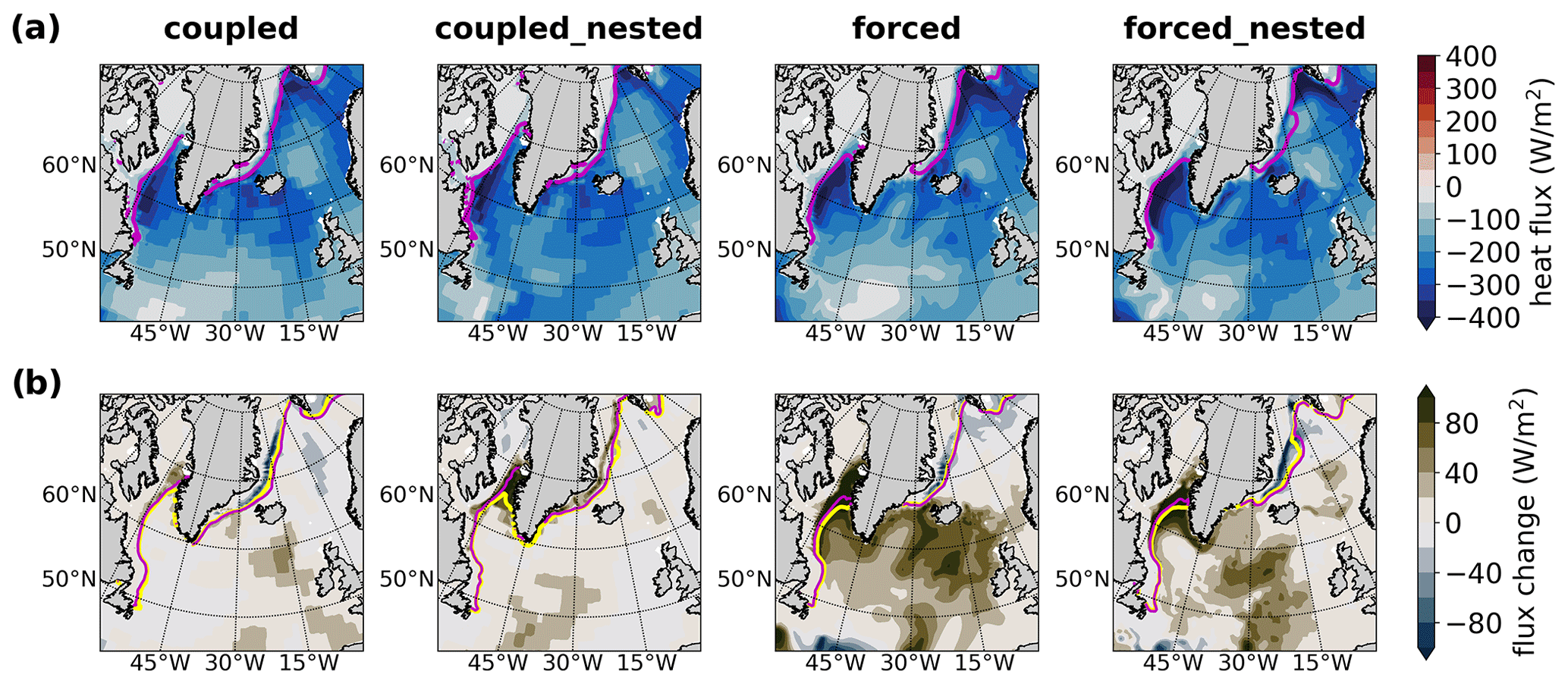
Figure 14 (a) Long-term mean surface heat flux (negative is ocean heat loss) averaged over December to February (DJF). (b) Response in surface heat flux (positive means reduced heat loss) to freshwater perturbation, DJF mean. Magenta and yellow lines depict the sea-ice edge (15 % ice concentration contour) for the reference and perturbed states, respectively.

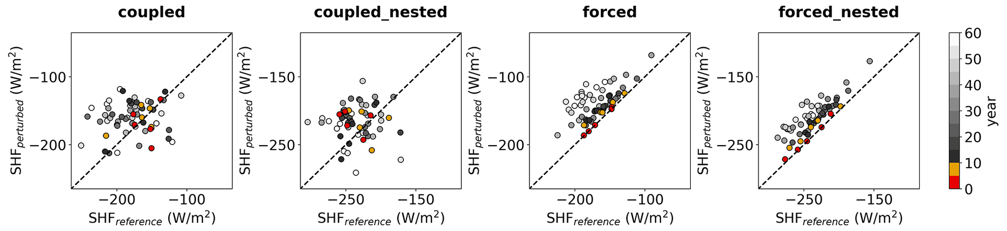
Figure 15 Changes in surface heat flux (SHF) due to the freshwater perturbation. SHF is averaged over the ENA region (see Fig. 8) and over December to February (DJF). Circles for each of the first 62 years of the perturbed simulations vs. the respective years of the reference runs are displayed. Years 1–5 and 6–10 are highlighted in red and yellow, respectively. Axis scales are shifted by −50 W m⁻² for the two nested configurations. The dashed line depicts the 1:1 line.

Surface heat flux

We focus our analysis of the surface heat flux (SHF) on the winter season, averaging from December to February (DJF), which dominates the annual mean. Heat loss from the ocean to the atmosphere across the SPNA during fall and winter increases upper-ocean density and hence plays an eminent role in preconditioning the ocean for deep convection, with a peak in March. All four model configurations show similar patterns and magnitudes of SHF in their mean states (Fig. 14a). Maximum heat loss, which exceeds 400 W m⁻², is found in the northwestern Labrador Sea along the sea-ice edge and similarly in the Nordic Seas, as well as over the path of the Atlantic water. However, a vast area of major air–sea heat exchange is in the northeastern SPNA. The block-like structure in the SHF output of the coupled configurations is due to the surface fluxes being computed on the coarser grid of the atmospheric model at a horizontal resolution of about 1.9^∘ (but stored on the ocean model grid at 0.5^∘). While the large-scale pattern is very similar in all reference simulations, we note a difference in the region of the Northwest Corner, east of Newfoundland. In the non-eddying configurations, which feature a strong SST cold bias in this region (see Fig. 3), a near-zero SHF can be found. In contrast, the coupled–nested configuration, almost completely lacking this bias, simulates a heat loss of around 200–250 W m⁻² in this region.

In the coupled experiments, the atmosphere can adjust to ocean surface conditions. In contrast, the atmosphere may act as an infinite source (or sink) of energy to the ocean in the forced experiments. This is well expressed by the DJF-mean SHF change presented in Fig. 14b. The two coupled experiments yield SHF changes of less than 20 W m⁻² in most of the SPNA, and nowhere do they yield changes of more than 50 W m⁻². The forced experiments, however, present with a distinct pattern of SHF increase, which here means reduced ocean heat loss. The pattern very much resembles the cooling pattern of upper-ocean temperature shown in Fig. 6b. Without an adjustment in atmospheric temperatures, the upper-ocean cooling in response to the freshwater perturbation and AMOC weakening reduces the temperature difference between ocean and atmosphere, which is below SST in winter, and thus yields a reduced heat loss of up to 100 W m⁻² across the entire SPNA, with a maximum on its eastern side. The SHF difference between the perturbed and reference run of the forced simulations remains positive (i.e., in a state of reduced heat loss) continuously throughout the experiment (Fig. 15). This shift evolves slowly over the first decade after perturbation onset (red and yellow circles). In contrast, internal variability in air–sea exchange dominates in the coupled system, and SHF differences of opposing sign are found. We also note a consistently larger heat loss by the two eddying configurations compared to the non-eddying ones, ranging from −250 to −150 W m⁻² rather than −200 to −100 W m⁻² (Fig. 15), which we attribute to sharper SST gradients from mesoscale filaments, a generally wider NAC, and a stronger AMOC in the nested configurations. The positive SHF anomalies in the freshwater perturbation experiments (Fig. 14b) are tightly associated with a reduction in the upward surface freshwater flux (evaporation minus precipitation, not shown). This provides another positive feedback favoring further AMOC weakening, particularly in the forced experiments.

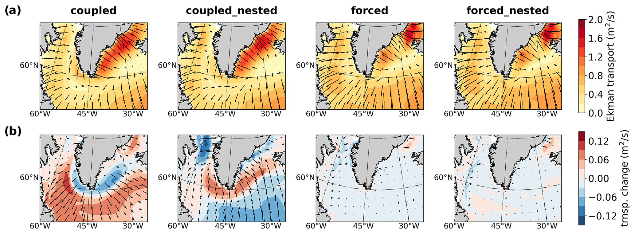
Figure 16 (a) Long-term annual-mean Ekman transport magnitude (colored contours) and direction (arrows, length relates to magnitude). (b) Response in Ekman transport to freshwater perturbation.

Ekman transport

The Greenland high- and Iceland low-pressure systems create predominant northeasterly winds over the continental shelf in the Irminger Sea. As a result, onshore downwelling-favorable Ekman transport (Fig. 16a) confines freshwater carried with the EGC (and its coastal sibling, the EGCC) to the shelf and shelf break (Fig. 5a). This is present in the atmospheric fields applied to the forced experiments, as well as in the coupled configuration, with the latter showing 30 %–40 % larger Ekman transport magnitudes. Over the WGC region, this is different. The coupled atmosphere tends to extend the low-pressure regime into the Labrador Sea, creating a similar gradient towards the Greenland high, which drives onshore Ekman transport here as well. In contrast, the forced simulations feature realistic offshore Ekman transport, pushing fresh polar waters away from the shelf. We consider this a major cause for finding a generally fresher upper ocean in the central Labrador Sea of the two forced experiments and much fresher conditions on the Labrador Sea shelf of the coupled simulations (Fig. 9).

While there is only negligible wind stress change in response to the freshwater perturbation in the two forced experiments, both coupled experiments yield a slight weakening of the Icelandic low, showing sea-level pressure increases of 0.5–1.0 hPa over the Labrador and Irminger seas, with a stronger increase in the non-eddying experiment (not shown). In the latter, this results in a weakening of the onshore Ekman transport in the WGC and Irminger Sea regions (Fig. 16b). Interestingly, the opposite is the case in the coupled–nested experiment, which may be related to the southward expansion of the sea-ice edge along the west coast of Greenland and associated surface heat flux reduction, which only emerge in the coupled–nested but not the coupled experiments and yield a local wind stress reduction over the Davis Strait (Figs. 14b and 16b). The particular reinforcement of the onshore Ekman transport over the WGC adds to the lack of eddy mixing and further limits the leakage of freshwater from the boundary current into the interior Labrador Sea in the coupled–nested configuration.

Summarizing, there certainly is a non-negligible influence on wind stress by an interactive atmosphere, which seems to reside less in a large-scale response to the broad surface cooling of the SPNA but rather in differences in critical locations. In our case, this aligns with a wind bias also crucial for the mean state of the model directly affecting deep-water formation. Although we cannot completely rule out an influence by the initial ocean mean states or climate conditions, we conclude that the damping of the surface heat and freshwater flux feedbacks in the coupled experiments is the main reason for their weaker AMOC response in comparison to their forced companion experiments.

4 Discussion

As the mass balance of the Greenland Ice Sheet grows increasingly negative, the impact thereof on the ocean has become a major topic for the SPNA community. The meltwater is difficult to detect by oceanographic observations and hence has led to an enhanced interest in numerical model simulations to project the near-term implications. As we note in the Introduction, the potential for GrIS mass loss having a significant long-term and large-scale impact on ocean circulation and sea level has been explored in many model studies before – like we did in Martin et al. (2022). However, the subtle beginnings and regional effects, as they may have occurred over the last decade already, likely require very sophisticated, high-resolution, strongly eddying, and even coupled models. This is what we argue for in the following. We also keep the focus on the SPNA, as this is where we can expect changes to show first.

To set the stage, we use the recently observed shift in deep convection from the Labrador Sea to the Irminger Sea as an example (de Jong et al., 2018; Zunino et al., 2020; Rühs et al., 2021). Rühs et al. (2021) argued for a potential role of enhanced Greenland runoff in this shift and showed that salinity anomalies in the northern part of the Labrador Sea correlate well with those in the EGC, particularly its coastal branch, which carries most of the runoff. Strongly eddying models have been used to show that WGC eddies are essential for this connection (Böning et al., 2016; Castelao et al., 2019; Georgiou et al., 2019). According to the model analysis of Rühs et al. (2021), the recent extreme freshening of the eastern North Atlantic (Holliday et al., 2020) arrives a little farther south, to the central Labrador Sea, being advected with the Irminger Current located slightly further offshore. Again (sub-)mesoscale processes play a role in connecting boundary current, deep convection, and downwelling (Georgiou et al., 2019; Tagklis et al., 2020). Recent freshening by polar water, runoff, and Atlantic water salinity anomalies may thus have contributed to hindering deep convection in the northwestern Labrador Sea. Recently enhanced deep convection in the Irminger Sea (Rühs et al., 2021) may have compensated for a lack of deep-water formation in the Labrador Sea and hence offset an impact by recently increased runoff from Greenland. In this respect, it is an intriguing feature of our coupled simulations that deep convection expands considerably southeast and east of Cape Farewell into the Irminger Sea (Fig. 7b). We do not find such response in the forced experiments. In contrast to forced simulations by Böning et al. (2016) and Rühs et al. (2021), the atmospheric forcing we apply here neither includes the recent increase in Greenland runoff nor matches with the applied freshwater perturbation.

Atmospheric coupling

With respect to the role of atmospheric feedback and forcing, our experiments are tailored towards the objective of whether forced ocean (and sea-ice) simulations can be used to demonstrate and diagnose the impact of enhanced GrIS melting in the ocean. But the question regarding the influence of ocean–atmosphere interaction is not that simply answered.

On the one hand, our results show the strong influence of a missing negative temperature feedback for stabilizing the AMOC in forced experiments (see Rahmstorf and Willebrand, 1995; Gerdes et al., 2006; Griffies et al., 2009), in which the AMOC weakens twice as much as in the coupled experiments (Table 2). This is despite differences in climate mean state (pre-industrial for coupled vs. present in forced experiments), spinup length (1600 vs. 30 years, i.e., separation from observation-based initial ocean status), and surface salinity restoring (none vs. weak). The coupled model develops a negative or positive salinity bias above or below 600 m during the extended spinup (Matthes et al., 2020, their Fig. 14). This may help to maintain the mode of recurring deep convection, making the coupled ocean less susceptible to the prescribed moderate freshwater perturbation. In both forced freshwater-release experiments, the cooling of the subpolar North Atlantic reduces evaporation, while precipitation is unaffected, being prescribed, resulting in an increase in the net surface freshwater flux. The surface salinity restoring acts quite efficiently against this increase on a basin scale with similar magnitude but opposite sign. The restoring thus mitigates part of the missing negative temperature feedback in the forced experiments by compensating for the temperature feedback on the surface freshwater flux (cf. Griffies et al., 2009). Nevertheless, the negative temperature feedback is still largely reduced, as surface heat fluxes are unaffected by the salinity restoring. However, we cannot exclude a significant influence by the ocean and climate mean states, which differ between coupled and forced experiments.

On the other hand, to unambiguously show the influence of ocean–atmosphere interaction on the response of the climate system to such enhanced freshwater input, the forced experiments would need to be conducted using the surface fluxes of the coupled control experiment, as has been done by Stammer et al. (2011). Interestingly, our results disagree with those of Stammer et al. (2011), though the arguments are similar. In our setup, the coupled configuration is less sensitive to the freshwater perturbation than the forced one. We see a similar causality of enhanced heat loss associated with enhanced precipitation over the SPNA, supporting a further weakening of the AMOC just like Stammer et al. (2011) but in the forced instead of the coupled experiment. While upper-ocean cooling and freshening in their forced ocean-only experiment is considerably weaker than in their coupled one, larger changes in surface fluxes over the SPNA in our forced experiment also drive greater cooling and freshening compared to our coupled one (Figs. 6b and 5b). We suspect that this opposing outcome is due to computing the surface fluxes in the ocean model, prescribing atmosphere temperature and winds from an unrelated reanalysis rather than prescribing surface fluxes of a related, unperturbed coupled simulation. This may seem trivial but is an important argument for taking atmosphere feedback into account when quantifying the impact of current and future increases of freshwater input to the SPNA using models.

For studying and projecting the impact by GrIS mass loss using a coupled climate or ocean-only model, the representation of the coastal winds around Greenland will have major implications on the results of the simulation, too. As shown here but also by earlier studies (Luo et al., 2016; Schulze Chretien and Frajka-Williams, 2018; Castelao et al., 2019; Duyck et al., 2022), upwelling-favorable Ekman transport plays a significant role in spreading relatively fresh coastal waters offshore into the Labrador and Irminger seas. Forcing an ocean model with reanalysis winds may thus yield a better representation of the Ekman transport, an issue that may be overcome by coupling with a high-resolution atmosphere component.

Role of mesoscale eddies

Böning et al. (2016) investigated spreading of Greenland meltwater in an eddy-permitting ($\mathrm{1}/\mathrm{4}$^∘) and a strongly eddying ($\mathrm{1}/\mathrm{20}$^∘) ocean-only simulation and found that significantly more meltwater entered and accumulated earlier in the central Labrador Sea in the strongly eddying model. At first glance, our results seem contradictory with the greater freshening (Fig. 5) and higher meltwater concentrations (Fig. 13, 0–200 m) in this region found in the non-eddying models presented here. However, the non-eddying model presented here uses the GM parameterization to account for the effect of missing eddies, whereas the $\mathrm{1}/\mathrm{4}$^∘ model of Böning et al. (2016) did not include such parameterization. Further, our eddying model using a grid resolution of 1/10^∘ (compared to $\mathrm{1}/\mathrm{20}$^∘ in Böning et al., 2016) only features some larger eddies, so-called Irminger rings or WGC eddies, which carry relatively fresh water from the boundary current into the interior Labrador Sea and therefore play a role in preconditioning of deep convection, but not the many smaller ones, which are also crucial for the restratification process after deep convection in winter (Rieck et al., 2019). The WGC eddies resolved in our model are not numerous and hence not sufficient for bringing enough meltwater to the deep-convention sites to achieve results comparable to Böning et al. (2016). In a similar comparison of 1 and $\mathrm{1}/\mathrm{10}$^∘ model configurations, Weijer et al. (2012) already found that stronger boundary currents keep the freshwater anomaly away from the deep-convection sites in the eddying model. Dukhovskoy et al. (2016) also highlight the importance of eddy fluxes for Greenland meltwater runoff to enter the interior Labrador Sea in a model intercomparison involving similar ocean grid resolutions. This observation gains relevance as the global climate modeling community of the Coupled Model Intercomparison Project (CMIP) increasingly employs grid resolutions of $\mathrm{1}/\mathrm{4}$–$\mathrm{1}/\mathrm{12}$^∘ without eddy parameterizations, which is insufficient for regions of, for instance, deep- and bottom-water formation. We consider implementation of scale-aware eddy parameterizations, such as those proposed by Jansen et al. (2019), to be a promising solution for future application in high-resolution but not quite Rossby-radius-resolving models.

Biastoch et al. (2021) and Yeager et al. (2021) noted the importance of explicitly simulating mesoscale dynamics for an improved representation of the transport of Denmark Strait overflow water and the maintenance of its characteristics along the way for forced ocean-only and coupled climate model simulations, respectively. Our results clearly support this and stress the relevance of more accurately simulating the boundary current in addition to the overflow itself for reducing dilution of this crucial water mass on its way to the Labrador Sea. Gillard et al. (2022) recently highlighted the importance of vertical model grid resolution and an associated improved representation of the local topography for the exchange between the WGC and the interior Labrador Sea, an aspect our nested simulations do not reflect, as the vertical resolution of 46 levels is the same as in the non-eddying configuration. In addition, we note that our forced experiments show a higher correlation between AMOC strength and the overflow than the coupled ones, though the latter tend to have a slightly greater overflow water density. With respect to the above discussion, we speculate that the atmospheric fluxes have significant influence on this. It is likely that the much shorter spinup of the forced experiments also plays a role. After more than 1500 years, the coupled experiments have certainly drifted away from the observed initialization state, whereas the initialization may still have a beneficial effect on the forced configurations.

Our results are in line with the notion that explicitly simulating mesoscale eddies – rather than parameterizing their effect – does not significantly impact the response of the AMOC to global warming or freshwater anomalies. This specifically holds for the magnitude of the response and less for the adjustment timescale (similarly to Weijer et al., 2012). Winton et al. (2014) noted that AMOC state and variability are more important for the model's sensitivity than grid resolution, and Gent (2018) summarizes studies comparing non-eddying and eddying models for their AMOC sensitivity to buoyancy forcing and finds clear evidence for neither the AMOC being more sensitive in strongly eddying models nor for grid resolution as a dominant factor. Hirschi et al. (2020) and Jüling et al. (2021) have recently added evidence along these lines. However, like earlier studies (e.g., Weijer et al., 2012; Böning et al., 2016; Jüling et al., 2021), our experiments show that redistribution of meltwater and response patterns to enhanced input thereof become significantly more realistic with increasingly strong eddying simulations. The realistic simulation of processes in the deep-water formation regions requires grid resolutions of $\mathrm{1}/\mathrm{20}$^∘ or finer to resolve the necessary eddy spectrum (Böning et al., 2016; Rieck et al., 2019; Castelao et al., 2019; Georgiou et al., 2019; Tagklis et al., 2020; Pennelly and Myers, 2022). In turn, this suggests that the above conclusion of the eddying capability of the model having little impact on an AMOC response to buoyancy forcing in the SPNA might be premature and based on simulations with still-insufficient eddy presence.

Lastly, we argue that systematic model configuration comparisons like the one presented here are essential to understand the influence of different model components and parameterizations. However, our study shows that such systematic comparisons are difficult to carry out. Coupled and forced models naturally have different mean states. Should model parameters be optimized for each configuration or rather kept unchanged for a fair comparison? Grid resolution of each model component plays a role, too. Which resolution is sufficient for completely abandoning a related parameterization, such as GM for eddies? The presented results can certainly qualitatively support the assessment of model projections on AMOC weakening in a warming climate and, to some degree, also provide quantitative guidance, though each model has its own sensitivity.

5 Summary and conclusions

A systematic set of freshwater-release experiments with coupled climate and forced ocean-only model configurations using eddy parameterization and explicit simulation of mesoscale features was carried out for understanding the role of atmospheric feedbacks and mesoscale eddies in the ocean's response to enhanced Greenland runoff. We find an interactive atmosphere to play a major role in stabilizing the AMOC against an overly strong decline in response to a multi-decadal increase in Greenland runoff. Our simulations demonstrate that mesoscale dynamics have a major impact on the regional response patterns everywhere, from the Labrador Sea to the subtropical gyre. We thus conclude that both processes should be considered for projections of regional North Atlantic changes in a warming climate.

The decline of the AMOC in the forced experiments is more than twice the magnitude of the response in the coupled ones. This agrees well with the one forced simulation in Swingedouw et al. (2013), simulating the strongest weakening among a set of six otherwise coupled models. We attribute this sensitivity to the dominance of the positive salinity feedback in the absence of a compensating temperature feedback when the atmosphere is not able to adjust to changes in SST (Griffies et al., 2009). Our results show up to an order of magnitude difference in the change in surface heat flux between the two configurations. This lends strong support to the understanding that the AMOC in ocean-only simulations is too sensitive to its own changes once triggered by external forcing, such as enhanced freshwater input.

Although having a minor impact on the response of AMOC strength – a large-scale integrated quantity – mesoscale dynamics play a major role in the regional distribution of and response to the freshwater added. This is due to improved representations of the North Atlantic Current, the boundary currents, and overflows in the eddying simulations. The effect of eddies in cross-frontal transport, i.e., “leaking” freshwater from the boundary current into the Labrador Sea, and restratification can be parameterized comparatively well in non-eddying simulations using, for instance, the GM method (Gent and McWilliams, 1990). Comparing our results with those of Böning et al. (2016), we find that meltwater concentrations in the central Labrador Sea, as simulated with a $\mathrm{1}/\mathrm{20}$^∘ strongly eddying model, are better matched by our $\mathrm{1}/\mathrm{2}$^∘ simulation applying GM than they are by the $\mathrm{1}/\mathrm{4}$^∘ one without GM used as reference by Böning et al. (2016). Export and recirculation of the freshwater with the subpolar gyre deviate significantly between non-eddying and eddying models. Here, our non-eddying simulation cannot capture sufficiently the westward propagation along the North American coast and rather simulates a massive eastward spreading near the Flemish Cap (Fig. 13). Further, the eddy parameterization fails in our case to achieve the same magnitude of exchange between subpolar and subtropical gyres as simulated by the eddying model. Obviously, the path and role of the North Atlantic Current as a strongly eddying current are less easily corrected by parameterization (Drews et al., 2015; Park et al., 2016).

We note that model sensitivity to a freshwater perturbation is further influenced by local processes, such as overflow dynamics, deep mixing, and wind conditions over the Greenland shelf (Ekman transport, tip jets). While atmospheric coupling is important for the large-scale response, coupled models with coarse atmosphere grid resolution, such as those used here, may have deficits in representing local winds, particularly in coastal regions. Unfortunately, the GrIS meltwater unfolds its impact on deep convection in the Labrador Sea, particularly through Ekman transport, resulting from wind conditions along the narrow continental shelf of Greenland (Luo et al., 2016; Schulze Chretien and Frajka-Williams, 2018). Thus, for the most realistic redistribution of Greenland freshwater in a model ocean, a sufficient resolution in both ocean and atmosphere is required.

Model experiments aiming at longer, such as centennial or millennial, timescales may perform well without resolving such processes, in particular when being used for studying responses on much broader basin-wide spatial scales. In this case, local processes can also be skipped by the concept of the hosing experiments prescribing the freshening to the entire subpolar region. We suspect the model mean state and internal variability to dominate sensitivity and response in this case, and local mixing processes become less important. Also, for the results presented here, we cannot rule out an influence by the mean state of the model configuration, i.e., the initialization and the spinup length. A priori, this will have a greater impact the smaller the freshwater perturbation, which in our case is only 0.05 Sv. For such moderate perturbation, Martin et al. (2022) already noted a significant influence by the internal variability of the climate system. Recent increases in freshwater flux off Greenland are even 5 times smaller.

Some of this may sound trivial, but it cannot be overly emphasized that the subpolar North Atlantic is a highly complex ocean region, and different models (or model configurations) may yield different responses to the same freshwater perturbation for different reasons. We conclude that, to seriously project the impact of enhanced Greenland runoff over the next decades, a high-resolution, near-Rossby-radius-resolving but at least $\mathrm{1}/\mathrm{20}$^∘ model is required. This is to resolve eddy processes important for restratification in the Labrador and Irminger seas, as well as dynamic processes at the Northwest Corner. Alternatively, scale-aware parameterizations for such processes need to be applied to and further developed for eddying but not quite Rossby-radius-resolving ocean models. In this, we agree with other recent assessments (Hewitt et al., 2020; Swingedouw et al., 2022). For projections beyond 5–10 years into the perturbed state, we see a necessity to include full ocean–atmosphere interaction to account for the compensating temperature feedback of a weakening AMOC. Ocean historical hindcast simulations being forced with atmosphere reanalysis include this feedback to the degree that the observed atmosphere is adjusted to a real ocean cooling.

Despite its rapid increase over the past 2 decades, Greenland meltwater runoff and solid ice discharge still are relatively minor players in the freshwater budget of the subpolar North Atlantic being influenced by Arctic Ocean export, salinity variations in the Gulf Stream, precipitation, and sea-ice melt. The AMOC will weaken under global warming – even without ice sheet melt (Weijer et al., 2020). A weaker AMOC is likely less sensitive to Greenland runoff (Swingedouw et al., 2015). Climate model experiments disagree on the potential impact of Greenland meltwater among all other consequences of global warming (e.g., Swingedouw et al., 2006; Mikolajewicz et al., 2007) but typically result in a weaker AMOC response than forced ocean models (Martin et al., 2022; Swingedouw et al., 2022). However, such coupled simulations should not be dismissed per se in favor of very high resolution ocean-only configurations, as recently conveyed by Swingedouw et al. (2022). Our results emphasize that large-scale atmosphere–ocean feedback and local winds are as important as simulating a strongly eddying ocean. Therefore, it remains a major challenge to answer the question of whether Greenland meltwater can potentially tip the scale on deep convection and when it might do so.

Appendix A: Selecting a reference period

Internal variability of the climate system has the potential to mask the response of the ocean to a moderate freshwater perturbation of 0.05 Sv, as demonstrated by Martin et al. (2022). For the present study, we have carefully chosen the time periods for computing the reference mean state and the perturbed state. We deliberately chose different approaches and periods for the coupled and forced experiments, as summarized at the beginning of Sect. 3. Here, we present the response in AMOC strength (Fig. A1) and in SST (Fig. A2) to support our approach.

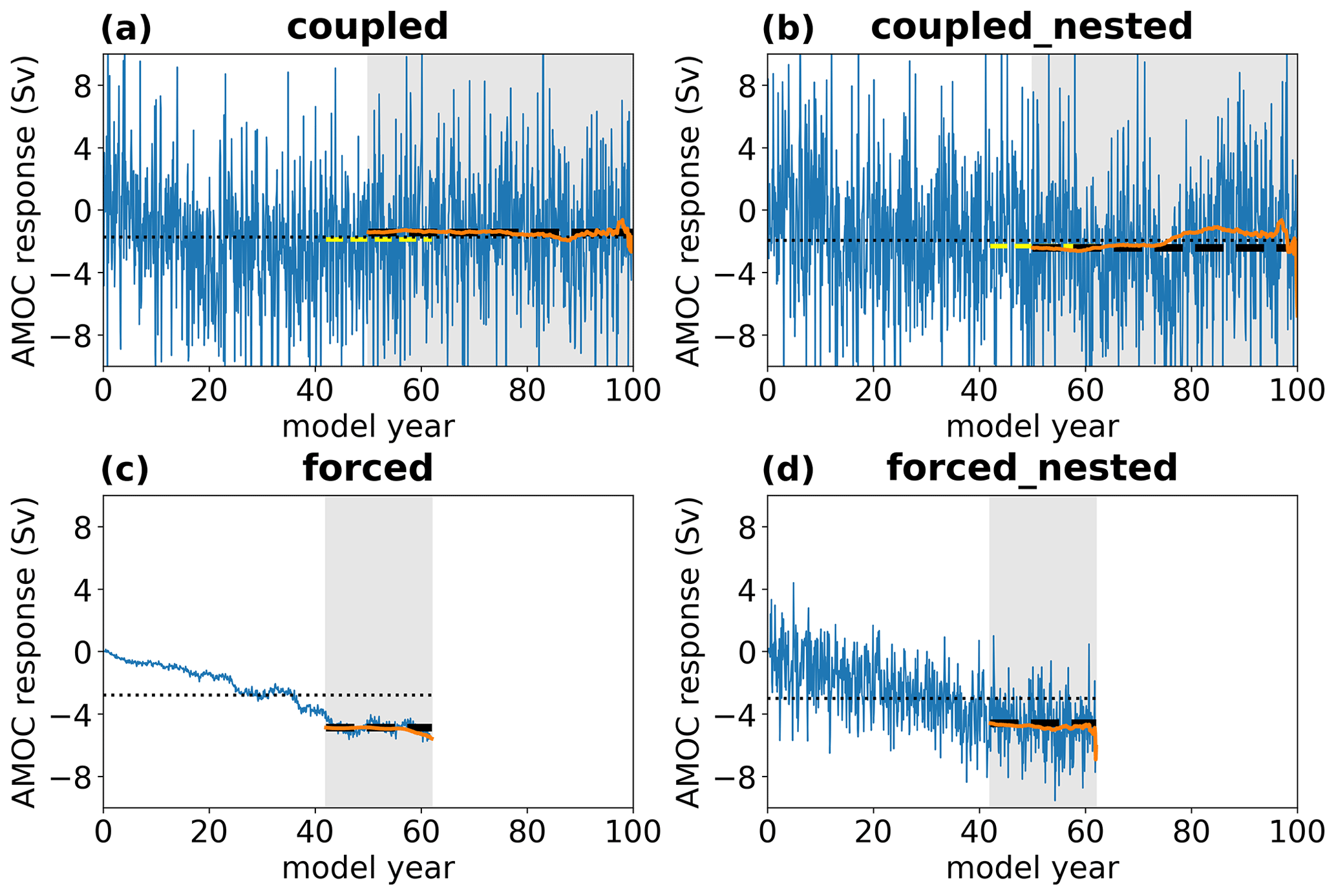
Figure A1 Difference in monthly mean AMOC strength (blue) between the perturbation experiment and the reference run of all four model configurations. Gray shading of the background marks the respective averaging periods for computing the response to the freshwater perturbation: years 51–100 for the coupled and years 43–62 for the forced experiments. The orange lines depict the running mean based on a boxcar window anchored at the end of the time series and expanding backwards in time. Dashed and dotted black lines indicate the overall mean for the response period (gray shading) and for the entire time series, respectively. The dashed yellow line in the upper panels depicts the mean of model years 43–62, which corresponds to the 20-year response period of the forced experiments (cf. lower panels).

Figure A1 offers a very clear impression of the internal variability simulated by the four model configurations. While the difference in AMOC strength between the perturbation experiment and the reference run is dominated by the weakening trend of the AMOC in the forced experiment, monthly and interannual variability is significantly larger in the forced–nested configuration. Since atmospheric variability is prescribed in these simulations, we can attribute the larger variability to the explicit simulation of mesoscale eddies. The eddy parameterization by Gent and McWilliams (1990) adds isopycnal mixing to non-eddying simulations, which otherwise would lack the conversion of potential to kinetic energy from local baroclinic instability, but misses additional sub-grid-scale effects and kinetic backscatter and hence rather acts to smooth variability, e.g., Zanna et al. (2017) and Hewitt et al. (2020). Despite the enhanced variability in the eddying simulation, we can still see the multi-decadal decline at the beginning of the experiment and that the trend in the two forced experiments is similar. In contrast, internal variability on monthly to decadal timescales dominates the time series of the two coupled configurations (Fig. A1 upper panels), and the decline at the beginning is difficult to identify. The former is also indicated by the standard deviations given in Table 2.

This behavior of internal variability motivated our decision to compute the response to the freshwater perturbation in two different ways for the coupled and forced experiments: by construction, the forced experiments experience the same temporal evolution of atmosphere-driven variability, and we can directly subtract the results of the perturbed experiment from the reference run for each time slice. The white noise added by the freely running atmosphere in the coupled experiments requires a statistical approach, and we compute mean state and response over longer time periods (see Fig. 2).

In the forced experiments, we can identify the AMOC strength to reach a seemingly stable state of difference from the reference run for the last 20 years. This is supported by computing a running mean of the AMOC strength difference between perturbed and reference run using a boxcar window always anchored at the end of the time series and expanding backwards in time. This mean stays stable until approximately year 40 (orange line in Fig. A1). Similarly, we find a relatively stable state of difference for the last 30+ years for the coupled experiments. As noted by Martin et al. (2022), the AMOC decline in the coupled experiments is difficult to separate from internal decadal variability, but the adjustment period is likely shorter than in the forced experiments due to the overall weaker response. Therefore, we simply use the second half of these experiments to reduce noise from internal variability for improved statistics.

The AMOC strength is an integrative quantity, and internal variability is typically even larger at the surface. We thus also present the influence of the averaging periods on the SST response in Fig. A2. Here, we distinguish the average over the entire simulation length (long-term mean) and averages over 20 and 50 years, i.e., over model years 43–62 (forced and coupled runs) and 51–100 (coupled runs only), as depicted in Fig. 2. Firstly, we note that the years 42–63 are slightly warmer compared to the respective long-term mean in the forced configurations. Secondly, 20- and 50-year reference periods differ in their spatial distribution of warm and cold anomalies with respect to the long-term mean in the SPNA of the coupled configurations. We consider these variations, which are mostly < 0.2 ^∘C and nowhere exceed 0.6 ^∘C, as uncertainty related to internal variability, i.e., the selection of the reference period. An exception is the Nordic Seas, where sea-ice retreat drives larger warming in the forced experiments.

The four lower rows in Fig. A2 show differences in SST between freshwater perturbation experiments and the reference runs. Using the forced experiments as an example, we see that the response in SST is biased low when using the long-term mean in both the reference and perturbation runs (EXPltm−REFltm). In contrast, warming in the Nordic Seas is overestimated and cooling in the SPNA is underestimated when comparing the last 20 years of the perturbation experiment with the long-term mean of the reference run (EXP20y−REFltm). Hence, the response to the freshwater perturbation is best isolated when subtracting the average of the exact same time period (EXP20y−REF20y) – at least in experiments where atmospheric forcing is prescribed. Since atmospheric variability cannot be controlled in coupled simulations and thus varies in each run, the optimal approach is to average over longer time periods to reduce the impact of internal variability but also to consider an adjustment period. The latter is typically shorter for surface properties than the deep ocean and for regions closer to the perturbation site, such as the SPNA in the present study (see Martin et al., 2022).

Figure A2 Reference mean state of sea-surface temperature (SST) from all four model configurations (top row) and deviations thereof depending on either time period or freshwater perturbation or both. The labeling on the left reads as follows: REF refers to the unperturbed reference experiments, and EXP refers to the freshwater perturbation experiments; temporal averaging is applied to either the entire run, yielding a long-term mean (ltm, 100 years for the two coupled, 62 years for the two forced configurations), or the years 43–62 (20 years) and 51–100 (50 years, coupled only) after onset of the perturbation.