Geostrophic adjustment on the midlatitude β plane

Analytical and numerical solutions of the linearized rotating shallow water equations are combined to study the geostrophic adjustment on the midlatitude β plane. The adjustment is examined in zonal periodic channels of width L_y=4R_d (narrow channel, where R_d is the radius of deformation) and L_y=60R_d (wide channel) for the particular initial conditions of a resting fluid with a step-like height distribution, η₀. In the one-dimensional case, where η₀=η₀(y), we find that (i) β affects the geostrophic state (determined from the conservation of the meridional vorticity gradient) only when $b=\cot \left({\mathit{\varphi }}_{\mathrm{0}}\right)\frac{R_{\mathrm{d}}}{R}\ge \mathrm{0.5}$ (where ϕ₀ is the channel's central latitude, and R is Earth's radius); (ii) the energy conversion ratio varies by less than 10 % when b increases from 0 to 1; (iii) in wide channels, β affects the waves significantly, even for small b (e.g., b=0.005); and (iv) for b=0.005, harmonic waves approximate the waves in narrow channels, and trapped waves approximate the waves in wide channels. In the two-dimensional case, where η₀=η₀(x), we find that (i) at short times the spatial structure of the steady solution is similar to that on the f plane, while at long times the steady state drifts westward at the speed of Rossby waves (harmonic Rossby waves in narrow channels and trapped Rossby waves in wide channels); (ii) in wide channels, trapped-wave dispersion causes the equatorward segment of the wavefront to move faster than the northern segment; (iii) the energy of Rossby waves on the β plane approaches that of the steady state on the f plane; and (iv) the results outlined in (iii) and (iv) of the one-dimensional case also hold in the two-dimensional case.

1 Introduction

It has long been established that large-scale flows in the ocean and atmosphere are in near-geostrophic balance, whereby the pressure gradient force is balanced by the Coriolis force (see, e.g., Gill, 1982, Sect. 7.6, and Vallis, 2017, Chap. 5). The fundamental theory of the way in which these flows transition from an initial unbalanced state to a geostrophically balanced state (known as geostrophic adjustment) is a cornerstone of geophysical fluid dynamics, as it is crucial for understanding the dynamics of the ocean and the atmosphere (see, e.g., Gill, 1982). Despite decades of research, the understanding of geostrophic adjustment is far from being complete.

The geostrophic adjustment theory was first studied in the 1930s, when Carl-Gustaf Rossby published pioneering works on the subject (Rossby, 1937, 1938). Rossby's work was extended in several papers, e.g., Blumen (1972) and Yacoby et al. (2021). However, as in Rossby's original studies, nearly all of these earlier studies addressed particular aspects (e.g., initial or boundary conditions) of the adjustment on the f plane; thus, their applicability to the real ocean is limited. Though the adjustment theory was extended to the equatorial β plane (Sect. 11.11 in Gill, 1982; Killworth, 1991; Rostami and Zeitlin, 2019, 2020) and to the sphere (Paldor and Dritschel, 2021), only marginal advances were made in extending the geostrophic adjustment theory to midlatitude β plane. In his discussion of the expected effect of β on the adjustment in midlatitudes, Blumen (1972, Sect. C2) commented that, on the β plane, the fluid should adjust to the quasi-geostrophic Rossby waves in the way that it adjusts to the steady-geostrophic state on the f plane. Similarly, in their study of the nonlinear adjustment process on the f plane, Reznik et al. (2001, Sect. 5) commented heuristically on the changes in the theory that should be expected when β≠0, but they have not developed a complete theory.

The waves that develop on the f and β planes during the adjustment process are determined by the boundary conditions and by the governing equations as follows: (i) in unbounded domains on the f plane, only Poincaré waves develop (Cahn, 1945); (ii) in channels on the f plane, Kelvin and Poincaré waves develop (Gill, 1976, 1982); (iii) in unbounded domains on the midlatitude β plane, Rossby and Poincaré waves develop (Blumen, 1972; Gill, 1982); (iv) on the equatorial β plane, Rossby, Kelvin, and Poincaré waves develop (Gill, 1982; Rostami and Zeitlin, 2019); and (v) in channels on the midlatitude β plane, Rossby, Kelvin, and Poincaré waves develop as in (iv), following from the combination of (ii) and (iii).

In wide channels on the midlatitude β plane, an alternate theory, the trapped-wave theory, was developed for Poincaré and Rossby waves (Paldor et al., 2007; Paldor and Sigalov, 2008; Paldor, 2015; see details in Sect. 3 below). These waves are called trapped since, in contrast to the classical harmonic waves, they are not spread over the entire meridional domain. Instead, they decay monotonically with latitude from their unique single maximum located near the equatorward boundary for low modes. The relevance of the trapped-wave theory was recently confirmed, using numerical simulations (Gildor et al., 2016) and satellite observations from the Indian Ocean (De-Leon and Paldor, 2017). The trapped-wave theory is employed in this study, as it underscores the effect of β on waves in wide channels (see Sects. 4.3, 5.2–5.3, and 6.2).

This paper examines the geostrophic adjustment theory in periodic zonal channels on the midlatitude β plane, and its outline is as follows: in Sect. 2, the governing equations, the numerical schemes used, and the setup of the problem are presented. In Sect. 3, we briefly compare the harmonic-wave theory and the trapped-wave theory and classify the width of the channels in which each of these theories is expected to be valid. For each theory, we summarize the analytical expressions for the dispersion relations and the eigenfunctions of both Poincaré and Rossby waves. In Sect. 4, we address the one-dimensional zonally invariant adjustment problem, when the initial height distribution, η₀, is a function of y. In Sect. 5, we address the two-dimensional adjustment problem, when η₀ is a function of x (the y dependence is explicit in f(y)). In both the one-dimensional and the two-dimensional cases, we examine the effect of β on the (i) geostrophic steady state (Sects. 4.1 and 5.1), (ii) waves' structure and spectrum (Sects. 4.3 and 5.2–5.3), and (iii) energetics of the adjustment process (Sects. 4.2 and 5.4). The paper ends with a discussion and summary in Sect. 6.

2 Setup of the problem

2.1 Governing equations

The (inviscid) linearized rotating shallow water equations (LRSWEs) are as follows:

$$\begin{array}{}\text{(1)}& {\displaystyle \frac{\partial u}{\partial t}}-f\left(y\right)v=-g{\displaystyle \frac{\partial \mathit{\eta }}{\partial x}},\text{(2)}& {\displaystyle \frac{\partial v}{\partial t}}+f\left(y\right)u=-g{\displaystyle \frac{\partial \mathit{\eta }}{\partial y}},\text{(3)}& {\displaystyle \frac{\partial \mathit{\eta }}{\partial t}}+H\left({\displaystyle \frac{\partial u}{\partial x}}+{\displaystyle \frac{\partial v}{\partial y}}\right)=\mathrm{0},\end{array}$$

where u and v are the velocity components along the x (zonal) and y (meridional) coordinates, respectively. η is the deviation of the fluid height from its mean value H, and g is the gravitational acceleration (or the reduced gravitational acceleration when the fluid is stratified). On the midlatitude β plane, the Coriolis frequency, f(y)=2Ωsin (ϕ) (where Ω is Earth's frequency of rotation and ϕ is the latitude), is expanded to the first order in y, in the vicinity of a mean latitude ϕ₀ (where y=0), such that

$$f\left(y\right)=f_{\mathrm{0}}+\mathit{\beta }y=\mathrm{2}\mathrm{\Omega }\left(\sin \left({\mathit{\varphi }}_{\mathrm{0}}\right)+{\displaystyle \frac{\cos \left({\mathit{\varphi }}_{\mathrm{0}}\right)}{R}}y\right),$$

where R, as mentioned above, is Earth's mean radius.

To reduce the number of free parameters in the problem, we scale t on $f_{\mathrm{0}}^{-\mathrm{1}}$, (x,y) on the radius of deformation, $R_{\mathrm{d}}=\sqrt{gH}/f_{\mathrm{0}}$, η on the initial disturbance amplitude $\stackrel{\mathrm{̃}}{\mathit{\eta }}$, and (u,v) on $\stackrel{\mathrm{̃}}{\mathit{\eta }}\sqrt{gH}/H$. This scaling guarantees that the amplitude of η(t=0) is 1 and yields the following non-dimensional equations:

$$\begin{array}{}\text{(4)}& {\displaystyle \frac{\partial u}{\partial t}}-(\mathrm{1}+by)v=-{\displaystyle \frac{\partial \mathit{\eta }}{\partial x}},\text{(5)}& {\displaystyle \frac{\partial v}{\partial t}}+(\mathrm{1}+by)u=-{\displaystyle \frac{\partial \mathit{\eta }}{\partial y}},\text{(6)}& {\displaystyle \frac{\partial \mathit{\eta }}{\partial t}}+{\displaystyle \frac{\partial u}{\partial x}}+{\displaystyle \frac{\partial v}{\partial y}}=\mathrm{0}.\end{array}$$

This system contains the single free parameter (the non-dimensional β), defined as follows:

$$b={\displaystyle \frac{\mathit{\beta }{R}_{\mathrm{d}}}{f_{\mathrm{0}}}}=\cot \left({\mathit{\varphi }}_{\mathrm{0}}\right){\displaystyle \frac{R_{\mathrm{d}}}{R}}.$$

It should be noted that, formally, this scaling applies to the Northern Hemisphere, where ϕ₀>0 i.e., f₀>0. In the Southern Hemisphere, a minus sign should be added to the scales of x, y (i.e., to R_d), and t, while the parameter b and the variables u, v, and η are unchanged.

Subtracting the y derivative of Eq. (4) from the x derivative of Eq. (5) yields the following vorticity equation:

$${\displaystyle \frac{\partial }{\partial t}}\left({\displaystyle \frac{\partial v}{\partial x}}-{\displaystyle \frac{\partial u}{\partial y}}\right)+(\mathrm{1}+by)\left({\displaystyle \frac{\partial u}{\partial x}}+{\displaystyle \frac{\partial v}{\partial y}}\right)=-bv,$$

which, together with Eq. (6), yields

$$\begin{array}{}\text{(7)}& {\displaystyle \frac{\partial q}{\partial t}}=-bv,q={\displaystyle \frac{\partial v}{\partial x}}-{\displaystyle \frac{\partial u}{\partial y}}-(\mathrm{1}+by)\mathit{\eta }.\end{array}$$

Following Gill (1982), the quantity $q/H$ is here termed the perturbation potential vorticity. This equation is used in Sect. 4.1 to find the geostrophic steady state.

2.2 Numerical scheme

The time-dependent system in Eqs. (4)–(6) is solved numerically, using the rotating shallow water (RSW) solver described in Gildor et al. (2016). Briefly, the finite difference numerical scheme employs a leapfrog time-differencing and central spatial differencing on an Arakawa C grid. A Robert–Asselin filter (Haltiner and Williams, 1980) is applied to suppress numerical modes. More details on this solver can be found in Gildor et al. (2016). The time step (Δt) and the grid spacing (Δx, Δy) were varied and are noted in Table 1 for each simulation (indicated in the table by the letters A–E). For several simulations, the results of the RSW calculations were compared to those obtained with the Massachusetts Institute of Technology General Circulation Model (MITgcm; see Marshall et al., 1997). In all such comparisons, the results obtained with the two models were identical, and for the most part, the RSW solver was less stable than the MITgcm and required a smaller Δt for given Δx and Δy, so it required a significantly longer computation time. Therefore, the longest simulation (D; see t_end in Table 1) was carried out using the MITgcm.

Table 1 Values of the numerical parameters (defined in Sect. 2.2–2.3) used in the five simulations denoted by the letters A–E.

^a Runtime. ^b This indicates that the number of cells in the zonal direction is four, which is the minimal value allowed by the solver (see Sect. 2.3). ^c The terms “wide” and “narrow” refer to a wide channel (L_y=60) and a narrow channel (L_y=4), respectively.

2.3 Channel configurations and boundary conditions

The adjustment is studied in a periodic zonal channel (i.e., where the channel walls of length L_x are aligned along the x direction and the channel width is L_y). When examining the one-dimensional (x-independent) problem (see Sect. 4), the number of cells in the zonal direction was set to the minimal value allowed by the solver, namely $L_x/\mathrm{\Delta }x=\mathrm{4}$. As expected, no variations in the zonal direction were developed in the numerical solution. When examining the two-dimensional problem (see Sect. 5), the channel length was varied from L_x=12 to L_x=120 (the length is noted in each case). The channel width was varied from L_y=4 in narrow channels to L_y=60 in wide channels. The origin of the y coordinate is chosen such that the channel walls are located at $y=\pm \frac{L_y}{\mathrm{2}}$. The boundary conditions at the channel's meridional boundaries are the vanishing of the normal velocities, such that

$$\begin{array}{}\text{(8)}& v=\mathrm{0}\mathrm{at}y=\pm {\displaystyle \frac{L_y}{\mathrm{2}}}.\end{array}$$

The boundary conditions at the channel's zonal boundaries are the periodicity of u, v, and η.

2.4 Initial conditions

Throughout this work, the fluid is assumed to be initially at rest (the subscript 0 in u, v, and η denotes initial values), such that

$$\begin{array}{}\text{(9)}& u_{\mathrm{0}}=v_{\mathrm{0}}=\mathrm{0}.\end{array}$$

In the one-dimensional case (Sect. 4), the initial surface height distribution, η₀, is a function of y and given by the following:

$$\begin{array}{}\text{(10)}& {\mathit{\eta }}_{\mathrm{0}}\left(y\right)=\mathrm{sgn}\left(y\right),\end{array}$$

while in the two-dimensional case (Sect. 5), η₀ is a function of x given by

$$\begin{array}{}\text{(11)}& {\mathit{\eta }}_{\mathrm{0}}\left(x\right)=\left\{\begin{array}{ll}\mathrm{0},& \mathrm{for}\left|x\right|>D,\\ \mathrm{1},& \mathrm{for}\left|x\right|<D,\end{array}\right.\end{array}$$

with $D=L_x/\mathrm{12}$. An initial-step condition, η₀(x)=sgn(x), is not addressed here, since it violates the assumed periodicity in the boundary conditions.

3 Harmonic- and trapped-wave theories in a channel

We now let the (u,v) velocity components and η in the LRSWE Eqs. (4)–(6) vary with x and t as a zonally traveling wave with a y-dependent amplitude, such that

$$(u,v,\mathit{\eta })=\left(\widehat{u}\left(y\right),\widehat{v}\left(y\right),\widehat{\mathit{\eta }}\left(y\right)\right)e^{i(kx-\mathit{\omega }t)},$$

where k is the wave's zonal wavenumber, and ω is its frequency. As shown in Paldor et al. (2007) and Paldor and Sigalov (2008), substituting these expressions for u, v, and η in Eqs. (4)–(6), eliminating $\widehat{u}$ and $\widehat{\mathit{\eta }}$, and neglecting second-order terms in by (i.e., the term $b^{\mathrm{2}}{y}^{\mathrm{2}}\widehat{v}$, noting that second-order terms in y have already been neglected in the first-order expansion of f(y)), yields the following Schrödinger eigenvalue equation for $\widehat{v}$:

$$\begin{array}{}\text{(12)}& {\displaystyle \frac{{\mathrm{d}}^{\mathrm{2}}\widehat{v}}{\mathrm{d}{y}^{\mathrm{2}}}}+(E-\mathrm{2}by)\widehat{v}=\mathrm{0},\end{array}$$

where $\widehat{v}$ is the eigenfunction and

$$\begin{array}{}\text{(13)}& E={\mathit{\omega }}^{\mathrm{2}}-k^{\mathrm{2}}-{\displaystyle \frac{bk}{\mathit{\omega }}}-\mathrm{1}\end{array}$$

is the eigenvalue. Note that since Eq. (12) is a typical Schrödinger equation, E can be interpreted as its energy level and −2by as its potential. In the high-frequency limit, $\frac{bk}{\mathit{\omega }}\ll \mathrm{1}$ and can be neglected, which yields the approximate dispersion relation for Poincaré waves, as follows:

$$\begin{array}{}\text{(14)}& {\mathit{\omega }}^{\mathrm{2}}=\mathrm{1}+k^{\mathrm{2}}+E.\end{array}$$

In the low-frequency limit, ω² can be neglected, which yields the approximate dispersion relation for Rossby waves.

$$\begin{array}{}\text{(15)}& \mathit{\omega }={\displaystyle \frac{-bk}{\mathrm{1}+k^{\mathrm{2}}+E}}\end{array}$$

The value of E, determined from the solution of the eigenvalue in Eq. (12), varies with b; for a small (respectively, large) value of b, it yields harmonic (respectively, trapped) waves.

For completeness, in the following subsections, we briefly outline the main properties of these two wave types and delineate the domains (b, L_y) in which each of these waves is expected to prevail.

3.1 Harmonic waves

In the harmonic-wave theory, the y-dependent term, −2by, is neglected in Eq. (12), which is solved by the following harmonic eigenfunctions:

$$\begin{array}{}\text{(16)}& {\widehat{v}}_n=\sin \left[{\displaystyle \frac{\mathit{\pi }(n+\mathrm{1})}{L_y}}\left(y+{\displaystyle \frac{L_y}{\mathrm{2}}}\right)\right],\end{array}$$

with the corresponding eigenvalues of

$$\begin{array}{}\text{(17)}& E_n={\left({\displaystyle \frac{\mathit{\pi }(n+\mathrm{1})}{L_y}}\right)}^{\mathrm{2}}.\end{array}$$

Substituting the expression for E_n found above in the dispersion relations (Eqs. 14 and 15) yields

$$\begin{array}{}\text{(18a)}& {\displaystyle }{\mathit{\omega }}^{\mathrm{2}}=\mathrm{1}+k^{\mathrm{2}}+{\left({\displaystyle \frac{\mathit{\pi }(n+\mathrm{1})}{L_y}}\right)}^{\mathrm{2}},\text{(18b)}& {\displaystyle }\mathit{\omega }={\displaystyle \frac{-bk}{\mathrm{1}+k^{\mathrm{2}}+{\left(\frac{\mathit{\pi }(n+\mathrm{1})}{L_y}\right)}^{\mathrm{2}}}}\end{array}$$

for harmonic Poincaré waves and harmonic Rossby waves, respectively.

3.2 Trapped waves

In the trapped-wave theory, the term −2by in Eq. (12) is retained. Defining

$$z\left(y\right)=-(\mathrm{2}b{)}^{-\mathrm{2}/\mathrm{3}}\left[E-\mathrm{2}by\right]$$

transforms Eq. (12) to the following Airy equation:

$$\begin{array}{}\text{(19)}& {\displaystyle \frac{{\mathrm{d}}^{\mathrm{2}}\widehat{v}}{\mathrm{d}{z}^{\mathrm{2}}}}-z\widehat{v}=\mathrm{0}.\end{array}$$

The general solution of Eq. (19) is a linear combination of Ai(z) that decays (faster than exponential) for z>0 and Bi(z) that grows (faster than exponential) for z>0. When $z\left(y=+\frac{L_y}{\mathrm{2}}\right)$ is sufficiently large, then $\mathrm{Ai}\left[z\left(y=+\frac{L_y}{\mathrm{2}}\right)\right]$ is negligibly small, so this function alone nearly satisfies the boundary condition at the northern wall, $y=+\frac{L_y}{\mathrm{2}}$, so the contribution of Bi(z) to the general solution has to be negligible. For example, for $z\left(y=+\frac{L_y}{\mathrm{2}}\right)=\mathrm{2}$, the value of Ai at the northern wall is $\mathrm{Ai}\left[z\left(y=+\frac{L_y}{\mathrm{2}}\right)\right]\le \mathrm{0.035}$, while the value of Bi(2)≈3.3 there. Thus, the Bi(z) term in the linear combination of the general solution must be 0 in order for the solutions to satisfy the boundary conditions.

The boundary condition at the southern wall, $y=-\frac{L_y}{\mathrm{2}}$, is satisfied by setting $z\left(y=-\frac{L_y}{\mathrm{2}}\right)$ to the nth 0 of Ai(z) (denoted as −ξ_n with ξ_n>0, since all zeros of Ai(z) are negative), and this condition determines the discrete eigenfunctions,

$$\begin{array}{}\text{(20)}& {\widehat{v}}_n=\mathrm{Ai}\left[(\mathrm{2}b{)}^{\mathrm{1}/\mathrm{3}}\left(y+{\displaystyle \frac{L_y}{\mathrm{2}}}\right)-{\mathit{\xi }}_n\right],\end{array}$$

with the corresponding eigenvalues,

$$\begin{array}{}\text{(21)}& E_n=(\mathrm{2}b{)}^{\mathrm{2}/\mathrm{3}}{\mathit{\xi }}_n-b{L}_y.\end{array}$$

Substituting this expression for E_n in the dispersion relations (Eqs. 14 and 15) yields

$$\begin{array}{}\text{(22)}& {\mathit{\omega }}^{\mathrm{2}}=\mathrm{1}+k^{\mathrm{2}}+(\mathrm{2}b{)}^{\mathrm{2}/\mathrm{3}}{\mathit{\xi }}_n-b{L}_y\end{array}$$

for trapped Poincaré waves and

$$\begin{array}{}\text{(23)}& \mathit{\omega }={\displaystyle \frac{-bk}{\mathrm{1}+k^{\mathrm{2}}+(\mathrm{2}b{)}^{\mathrm{2}/\mathrm{3}}{\mathit{\xi }}_n-b{L}_y}}\end{array}$$

for trapped Rossby waves.

As shown in Paldor and Sigalov (2008) and Gildor et al. (2016), the harmonic-wave theory provides accurate approximations for waves in narrow channels, while the trapped-wave theory does so in wide channels. The wide-channel scenario applies when $z\left(y=+\frac{L}{\mathrm{2}}\right)$ is increased above a threshold value, Z^∗, namely, when

$$z\left(y=+{\displaystyle \frac{L_y}{\mathrm{2}}}\right)=-(\mathrm{2}b{)}^{-\mathrm{2}/\mathrm{3}}\left[E-b{L}_y\right]>Z^{\ast },$$

where Z^∗ is sufficiently large. Using the expression for E_n (i.e., Eq. 21) leads to the following constraint on L_y:

$$\begin{array}{}\text{(24)}& L_y>(\mathrm{2}b{)}^{-\frac{\mathrm{1}}{\mathrm{3}}}\left(Z^{\ast }+{\mathit{\xi }}_n\right),\end{array}$$

which indicates that the higher the wave mode, n (and with it, value of ξ_n), the wider the channel should be for the trapped-wave theory to hold. As mentioned above, Z^∗ should be a sufficiently large number, and following the discussion at the beginning of this subsection, $Z^{\ast }=\mathrm{2}$ should be considered sufficiently large. We examine this subtle issue in Sect. 4.3 (see Eq. 38). The applicability of the trapped-wave theory to the ocean is discussed in Sect. 6.7.

Having established analytically the character of the transient waves in wide and narrow channels, we now turn to numerical solutions of the adjustment problem in one and two dimensions.

4 One-dimensional adjustment problem

When η₀ is a function of x only, then both the initial conditions (Eqs. 9–10) and the coefficients of the LRSWEs are independent of x, so the solutions can be assumed to be independent of x at all times. In this case, the governing equations, Eqs. (4)–(6), reduce to the following:

$$\begin{array}{}\text{(25)}& {\displaystyle \frac{\partial u}{\partial t}}-(\mathrm{1}+by)v=\mathrm{0},\text{(26)}& {\displaystyle \frac{\partial v}{\partial t}}+(\mathrm{1}+by)u=-{\displaystyle \frac{\partial \mathit{\eta }}{\partial y}},\text{(27)}& {\displaystyle \frac{\partial \mathit{\eta }}{\partial t}}+{\displaystyle \frac{\partial v}{\partial y}}=\mathrm{0},\end{array}$$

and Eq. (7) becomes

$$\begin{array}{}\text{(28)}& {\displaystyle \frac{\partial }{\partial t}}\left({\displaystyle \frac{\partial u}{\partial y}}+(\mathrm{1}+by)\mathit{\eta }\right)=bv.\end{array}$$

Substituting the continuity equation, Eq. (27), into the y derivative of Eq. (28) yields

$$\begin{array}{}\text{(29)}& {\displaystyle \frac{\partial }{\partial t}}\left({\displaystyle \frac{\partial {}^{\mathrm{2}}u}{\partial y^{\mathrm{2}}}}+(\mathrm{1}+by){\displaystyle \frac{\partial \mathit{\eta }}{\partial y}}+\mathrm{2}b\mathit{\eta }\right)=\mathrm{0},\end{array}$$

or, equivalently,

$${\displaystyle \frac{\partial }{\partial t}}\left({\displaystyle \frac{\partial q}{\partial y}}-b\mathit{\eta }\right)=\mathrm{0}.$$

This conservation equation for the meridional gradient of q (minus bη that originates from the y derivative of bv on the right-hand side of Eq. (28), which, according to Eq. (27), equals $-b\partial \mathit{\eta }/\partial t$) implies that the combination of time-dependent variables in the parentheses at time t equals their initial combination (denoted by the subscript “0”), such that

$$\begin{array}{}\text{(30)}& {\displaystyle \frac{\partial {}^{\mathrm{2}}u}{\partial y^{\mathrm{2}}}}+(\mathrm{1}+by){\displaystyle \frac{\partial \mathit{\eta }}{\partial y}}+\mathrm{2}b\mathit{\eta }={\displaystyle \frac{\partial {}^{\mathrm{2}}{u}_{\mathrm{0}}}{\partial y^{\mathrm{2}}}}+(\mathrm{1}+by){\displaystyle \frac{\partial {\mathit{\eta }}_{\mathrm{0}}}{\partial y}}+\mathrm{2}b{\mathit{\eta }}_{\mathrm{0}}.\end{array}$$

In contrast to the f plane, where q is locally conserved (i.e., it retains its initial value at each point), on the β plane, the conserved quantity is $\partial q/\partial y-b\mathit{\eta }$. Thus, while on the f plane Eq. (28) with b=0 yields the relation between the initial and final states, on the β plane, this relation is derived from the y derivative of the vorticity equation in the form of Eq. (30). Indeed, on the f plane, the conservation of q was employed in Gill (1976, Eqs. 4.7–4.8) and Gill (1982, Eqs. 7.2.8–7.2.10).

We note that in the dimensional form, the potential vorticity (PV) is given by the following (see, e.g., Vallis, 2017, Sect. 3.9.2):

$$\begin{array}{rl}Q& ={\displaystyle \frac{\frac{\partial v}{\partial x}-\frac{\partial u}{\partial y}+f\left(y\right)}{H+\mathit{\eta }}}\approx {\displaystyle \frac{\mathit{\zeta }+f}{H}}\left(\mathrm{1}-{\displaystyle \frac{\mathit{\eta }}{H}}\right)\\ & \approx {\displaystyle \frac{\mathrm{1}}{H}}\left(f+\mathit{\zeta }-f{\displaystyle \frac{\mathit{\eta }}{H}}\right)={\displaystyle \frac{f}{H}}+{\displaystyle \frac{q}{H}}\end{array}$$

and is conserved in a Lagrangian manner (but not necessarily locally) on both the f and β planes, such that

$$\begin{array}{}\text{(31)}& {\displaystyle \frac{\mathrm{D}Q}{\mathrm{D}t}}=\mathrm{0},\end{array}$$

where

$${\displaystyle \frac{\mathrm{D}}{\mathrm{D}t}}={\displaystyle \frac{\partial }{\partial t}}+u{\displaystyle \frac{\partial }{\partial x}}+v{\displaystyle \frac{\partial }{\partial y}}+w{\displaystyle \frac{\partial }{\partial z}}$$

is the material derivative, and $q/H$ is the dimensional form of the perturbation potential vorticity defined (in nondimensional form) in Eq. (7). Thus, Eq. (7) is, in fact, the linearized and nondimensional form of Eq. (31) that yields the local conservation law – Eq. (28) – when $\partial /\partial x=\mathrm{0}$.

4.1 Steady state

The steady (geostrophic) solution of Eqs. (25)–(26) (denoted with the subscript “g”) satisfies

$$\begin{array}{}\text{(32)}& v_{\mathrm{g}}=\mathrm{0}\end{array}$$

and

$$\begin{array}{}\text{(33)}& {\displaystyle \frac{\partial {\mathit{\eta }}_{\mathrm{g}}}{\partial y}}=-(\mathrm{1}+by)u_{\mathrm{g}}.\end{array}$$

No information beyond this geostrophic relation between u_g and η_g is contained in the system (Eqs. 25–27) when $\frac{\partial }{\partial t}=\mathrm{0}=v$. However, a second general relation between u and η is provided by Eq. (30) that expresses the conservation of the meridional gradient of vorticity, and this general relation applies also to the steady solutions. The geostrophic relation can be combined with the conservation of the meridional vorticity gradient to uniquely determine u_g and η_g. The system (Eqs. 30 and 33) can only be solved numerically by imposing relevant boundary conditions and solving the associated eigenvalue problem (we used the MATLAB bvp4c solver). The boundary conditions for u were derived as follows: substituting the boundary condition $v\left(\pm \frac{L_y}{\mathrm{2}}\right)=\mathrm{0}$ in Eq. (25) yields ${\left.\frac{\partial u}{\partial t}\right|}_{y=\pm L_y/\mathrm{2}}=\mathrm{0}$, so u retains its initial value at the boundaries, such that

$$\begin{array}{}\text{(34)}& u=u_{\mathrm{0}}=\mathrm{0}\mathrm{at}y=\pm {\displaystyle \frac{L_y}{\mathrm{2}}}.\end{array}$$

Note that, formally, the condition (Eq. 34) determines the vanishing of u(y,t) at the boundaries and not the vanishing of the steady-geostrophic u_g(y). However, since u_g is the averaged distribution (over many wave periods) of u, u_g must also satisfy the condition (Eq. 34). The boundary conditions for η_g were determined as follows: for large channels (L_y=60), we assume that the geostrophic state is confined to a relatively small area around x=0, such that

$$\begin{array}{}\text{(35)}& {\mathit{\eta }}_{\mathrm{g}}={\mathit{\eta }}_{\mathrm{0}}=\pm \mathrm{1}\mathrm{at}y=\pm {\displaystyle \frac{L_y}{\mathrm{2}}}.\end{array}$$

For narrow channels (L_y=4), we impose the condition

$$\begin{array}{}\text{(36)}& {\displaystyle \frac{\partial {\mathit{\eta }}_{\mathrm{g}}}{\partial y}}=\mathrm{0}\mathrm{at}y=-{\displaystyle \frac{L_y}{\mathrm{2}}},\end{array}$$

which follows from Eq. (33), since $u_{\mathrm{g}}(\pm L_y/\mathrm{2}=\mathrm{0})=\mathrm{0}$, and the condition

$$\begin{array}{}\text{(37)}& {\mathit{\eta }}_{\mathrm{g}}=-a\mathrm{at}y=-{\displaystyle \frac{L_y}{\mathrm{2}}},\end{array}$$

where the value of a is determined by mass conservation as

$$\underset{-L_y/\mathrm{2}}{\overset{L_y/\mathrm{2}}{\int }}{\mathit{\eta }}_g\mathrm{d}y=\underset{-L_y/\mathrm{2}}{\overset{L_y/\mathrm{2}y}{\int }}{\mathit{\eta }}_{\mathrm{0}}\mathrm{d}y=\mathrm{0}.$$

This mass conservation condition is applied as follows. We scan a finite range of a values from −1 to −0.3, with intervals of 0.005, and choose the value of a that yields the lowest absolute value (i.e., closest to 0) of the integral:

$$\underset{-L_y/\mathrm{2}}{\overset{L_y/\mathrm{2}}{\int }}{\mathit{\eta }}_g\mathrm{d}y.$$

Figure 1 compares the geostrophic solutions on the β plane (solid lines) and the f plane (dashed lines). In midlatitudes (${\mathit{\pi }}_{\mathrm{0}}=\mathit{\pi }/\mathrm{4}$), the value b=0.005 corresponds to R_d∼30 km, a typical oceanic value, whereas b=0.05 corresponds to R_d∼300 km, a typical atmospheric value. The figure clearly shows that the effect of β on the geostrophic state is relatively small and becomes significant only at large b values that are unacceptable for the midlatitude β plane, since $b{L}_y/\mathrm{2}\ge \mathrm{1}$ (i.e., $\mathit{\beta }{L}_y/\mathrm{2}\ge f_{\mathrm{0}}$ in dimensional notation). Such unacceptable cases are evident in Fig. 1 in the b=0.05 row of a wide channel (left column, middle panel; $b{L}_y/\mathrm{2}=\mathrm{1.5}$) and both columns of the b=0.5 row (bottom panels; $b{L}_y/\mathrm{2}=\mathrm{15}$ in the left panel and $b{L}_y/\mathrm{2}=\mathrm{1}$ in the right panel). Thus, in all acceptable values of b and L_y, the steady state on the f plane provides an accurate estimate of the same state on the β plane.

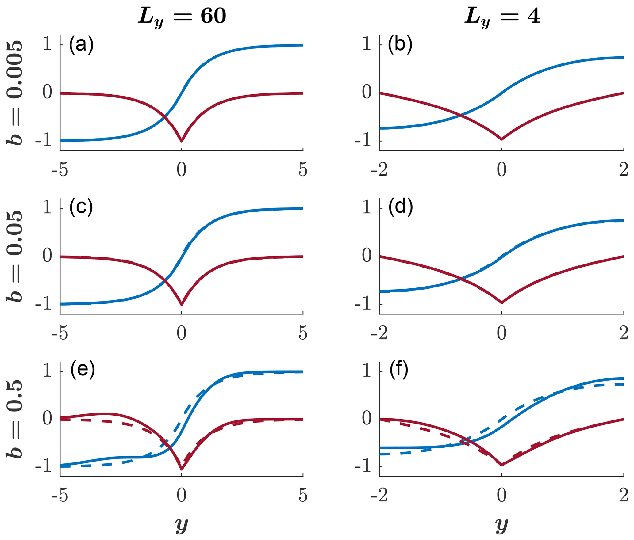
Figure 1 The spatial structure of the geostrophic steady state, η_g (blue) and u_g (red). Solid lines show the distributions for the indicated values of b, and dashed lines show the distributions for b=0 (i.e., on the f plane). (a, c, e) A wide channel. (b, d, f) A narrow channel. In all steady states, v=0. For b≤0.05, the solid lines coincide with the dashed lines. For the f plane, we use the analytic solutions (A31)–(A32) of Yacoby et al. (2021), with η_g(x) replaced by η_g(y) and v_g(x) replaced by −u_g(y).

4.2 Energy

Having analyzed the effect of β on the steady-geostrophic state, we turn to the examination of its effect on the energetics of the adjustment process. This analysis proved to be very informative on the f plane, where it quantifies the division between the potential energy and kinetic energy in the final state and between the waves and the final steady state (Yacoby et al., 2021). As we shall shortly see, the effect of β on the energy division is small for physically acceptable values of b.

Since the seminal study by Gill (1976), it has become common practice to analyze the energetics of the adjustment problem by calculating the energy conversion ratio as follows (see, e.g., Grimshaw et al., 1998; Fang and Wu, 2002; Yacoby et al., 2021):

$$\mathit{\gamma }={\displaystyle \frac{{\mathrm{KE}}_{\mathrm{g}}}{{\mathrm{PE}}_{\mathrm{0}}-{\mathrm{PE}}_{\mathrm{g}}}},$$

where ${\mathrm{KE}}_{\mathrm{g}}=\frac{\mathrm{1}}{\mathrm{2}}{\int }_{-L_y/\mathrm{2}}^{L_y/\mathrm{2}}{u}_{\mathrm{g}}^{\mathrm{2}}\mathrm{d}y$ is the total kinetic energy of the geostrophic state, ${\mathrm{PE}}_{\mathrm{g}}=\frac{\mathrm{1}}{\mathrm{2}}{\int }_{-L_y/\mathrm{2}}^{L_y/\mathrm{2}}{\mathit{\eta }}_{\mathrm{g}}^{\mathrm{2}}\mathrm{d}y$ is the total potential energy of the geostrophic state, and ${\mathrm{PE}}_{\mathrm{0}}=\frac{\mathrm{1}}{\mathrm{2}}{\int }_{-L_y/\mathrm{2}}^{L_y/\mathrm{2}}{\mathit{\eta }}_{\mathrm{0}}^{\mathrm{2}}\mathrm{d}y$ is the total potential energy of the initial state. Note that the total kinetic and potential energies are defined as the integral of the corresponding local values over the entire channel width L_y. Figure 2 shows γ as a function of b for L_y=60 (blue line and dots) and for L_y=4 (red line and dots). The value of γ is calculated in two ways (one shown by lines and the other by dots) that differ by the methods used for calculating the geostrophic state, η_g and u_g. The first method is that employed in Fig. 1; i.e., it solves Eqs. (30) and (33) using MATLAB's bvp4c routine. Prior to the calculation of the integral of $\frac{\mathrm{1}}{\mathrm{2}}{\mathit{\eta }}_{\mathrm{g}}^{\mathrm{2}}$ and $\frac{\mathrm{1}}{\mathrm{2}}{u}_{\mathrm{g}}^{\mathrm{2}}$ over the entire channel width (to calculate PE_g and KE_g), the values of η_g and u_g are spline-interpolated. The values of γ calculated in this way are shown by the blue (L_y=60) and red (L_y=4) lines. In the second method, η, u, and v are simulated using the RSW solver described in Sect. 2.2 (simulation A) and the simulated η and u values are averaged over many wave periods. The averages were calculated between t=0 and t=200, with intervals of 0.1 time units (i.e., intervals of 100Δt; see Table 1). Figure 2 shows that γ varies with b by no more than 10 % compared to the f plane values noted along the b=0 ordinate. In a narrow channel (L_y=4; red line and dots), the decrease in γ(b) is monotonic, while in a wide channel (L_y=60; blue line and dots), γ has a local maximum of ≈0.343 at b≈0.3.

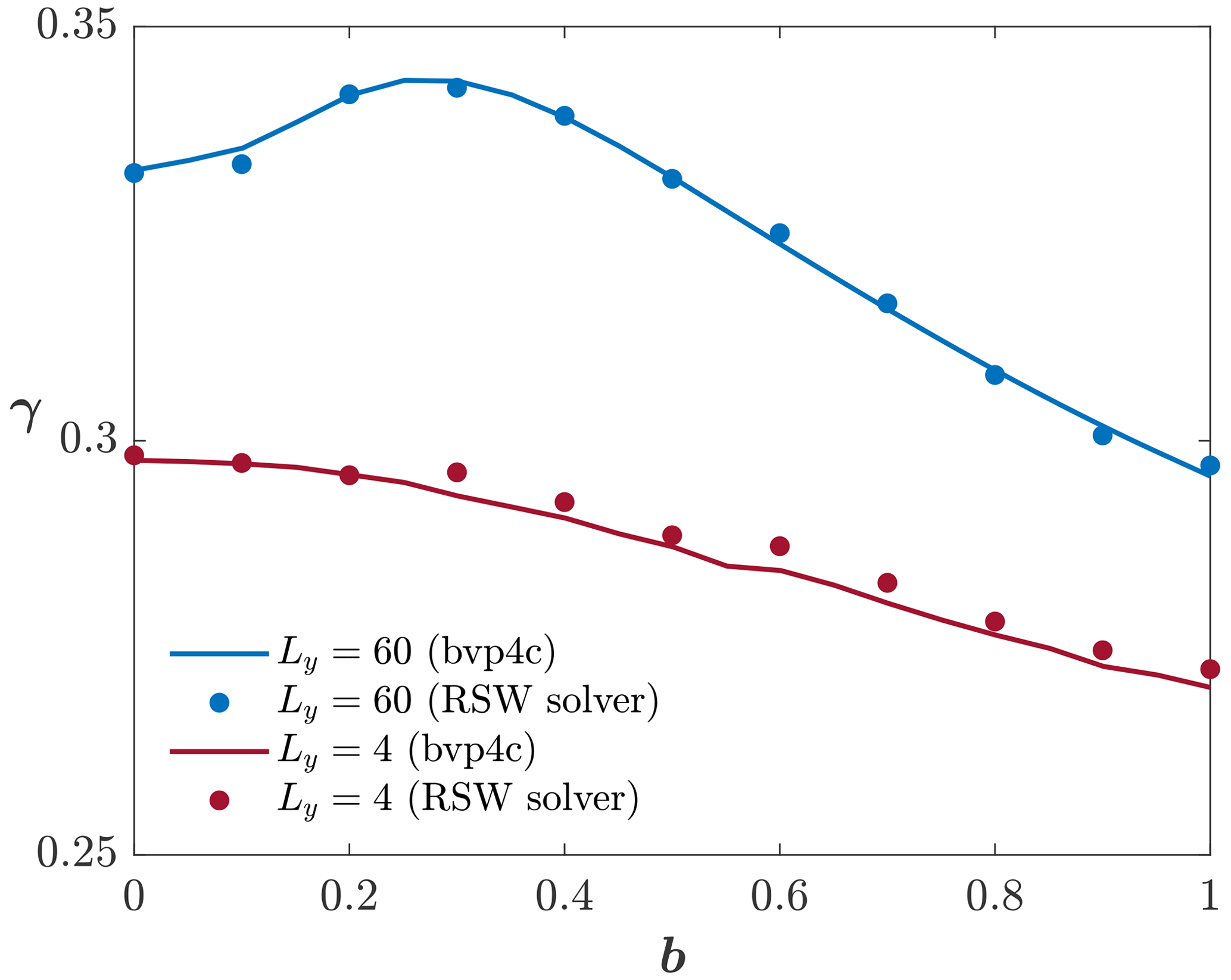
Figure 2 The energy conversion ratio, γ, as a function of b for L_y=60 (blue) and for L_y=4 (red). Lines show the values of γ based on the geostrophic state calculated using MATLAB bvp4c, as in Fig. 1. Dots show the values of γ when the geostrophic state is calculated using the RSW solver by taking the average of η and u, as detailed in the text.

4.3 Poincaré waves

The analysis of the v(y,t) field employs the empirical orthogonal function (EOF) method that examines the field's spatial and temporal patterns of variability (see, e.g., Björnsson and Venegas, 1997; Eshel, 2011, Chap. 11). We apply the EOF analyses to the v(y,t) field simulated by the RSW solver (simulation B). Henceforth, we choose b=0.005, a typical value in the ocean, where R_d∼30 km at ${\mathit{\varphi }}_{\mathrm{0}}=\mathit{\pi }/\mathrm{4}$.

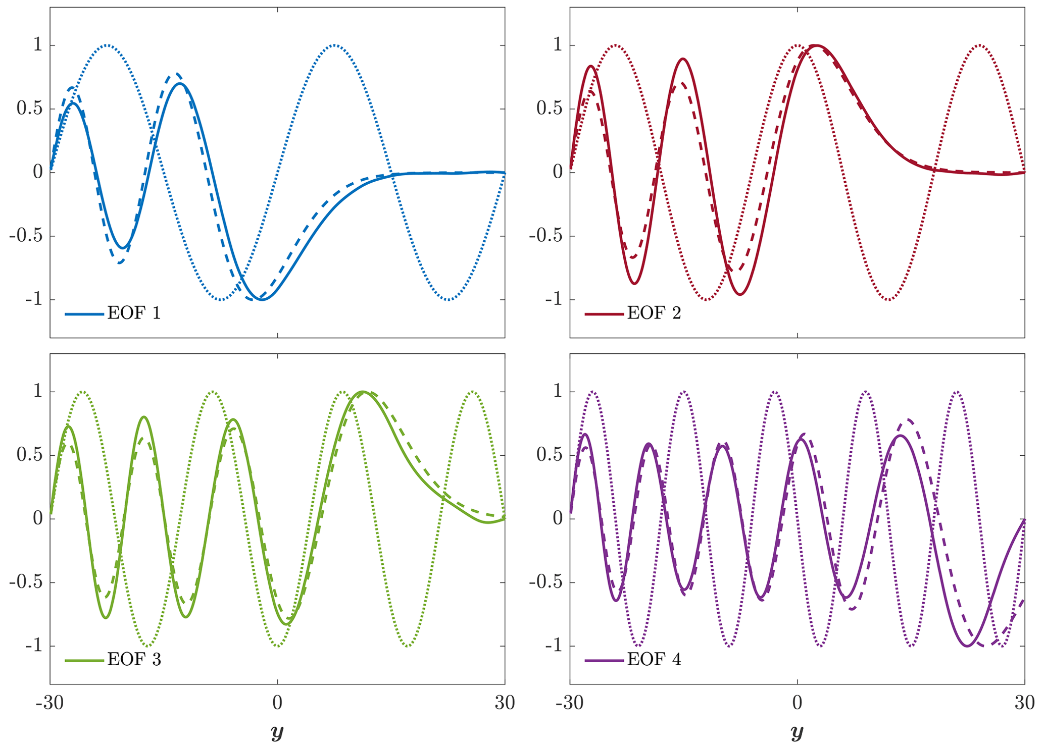
Figure 3 Solid lines show the first four EOFs of v(y,t) in a wide channel. Dashed lines show the Airy eigenfunctions for n=3 (blue), n=4 (red), n=6 (green), and n=9 (purple). Dotted lines show the harmonic eigenfunctions for the same modes. In this wide channel case, the EOFs resemble the Airy eigenfunctions.

The solid lines in Fig. 3 show the first four EOFs of v(y,t) in a wide channel (L_y=60) for b=0.005. Each EOF mode can be associated with a different wave mode by examining the number of nodal points; i.e., EOFs 1–4 are associated with wave modes n=3, 4, 6, and 9, respectively. The dashed lines show the Airy eigenfunctions given by Eq. (20) for n=3 (blue), n=4 (red), n=6 (green), and n=9 (purple), and the dotted lines show the corresponding harmonic modes given by Eq. (16) for the same mode numbers. All curves are normalized, such that the maximal absolute value of their amplitude equals 1 and their derivative at $y=-L_y/\mathrm{2}$ is positive.

Clearly, in a wide channel, the EOFs are very similar to the Airy eigenfunctions. However, there is a significant deviation between EOF 4 (solid purple) and its associated Airy eigenfunction (dashed purple) near the northern wall, $y=L_y/\mathrm{2}$. The reason for this deviation is the violation of the condition (Eq. 24) for large-mode numbers, i.e., when ξ_n is too large. The fact that the EOFs match the Airy eigenfunctions accurately for $n=\mathrm{3},\mathrm{4}$, and 6 but not so for n=9 results from the bound on the value of Z^∗ (set to 2, as discussed at the end of Sect. 3.2). Specifically, the condition (Eq. 24) implies the following:

$$\begin{array}{}\text{(38)}& (\mathrm{2}b{)}^{\mathrm{1}/\mathrm{3}}{L}_y-{\mathit{\xi }}_n>Z^{\ast }.\end{array}$$

For the values of L_y=60 and b=0.005 used here, the left-hand side of Eq. (38) equals 2.886 for n=6 (ξ₆=10.040), while for n=9 (ξ₉=12.829) it equals 0.098. The results shown in Fig. 3, where EOF 3 matches the n=6 mode in the channel nicely, while EOF 4 matches the n=9 mode only roughly, supports our choice of $Z^{\ast }=\mathrm{2}$ in Eq. (38). As could be expected, the mismatch between EOF 4 and the n=9 wave mode is maximal near the northern boundary, while inward of it, the match is acceptable throughout most of the domain. The results also show that harmonic waves do not yield acceptable approximations to the calculated EOFs in the wide channel for any mode number.

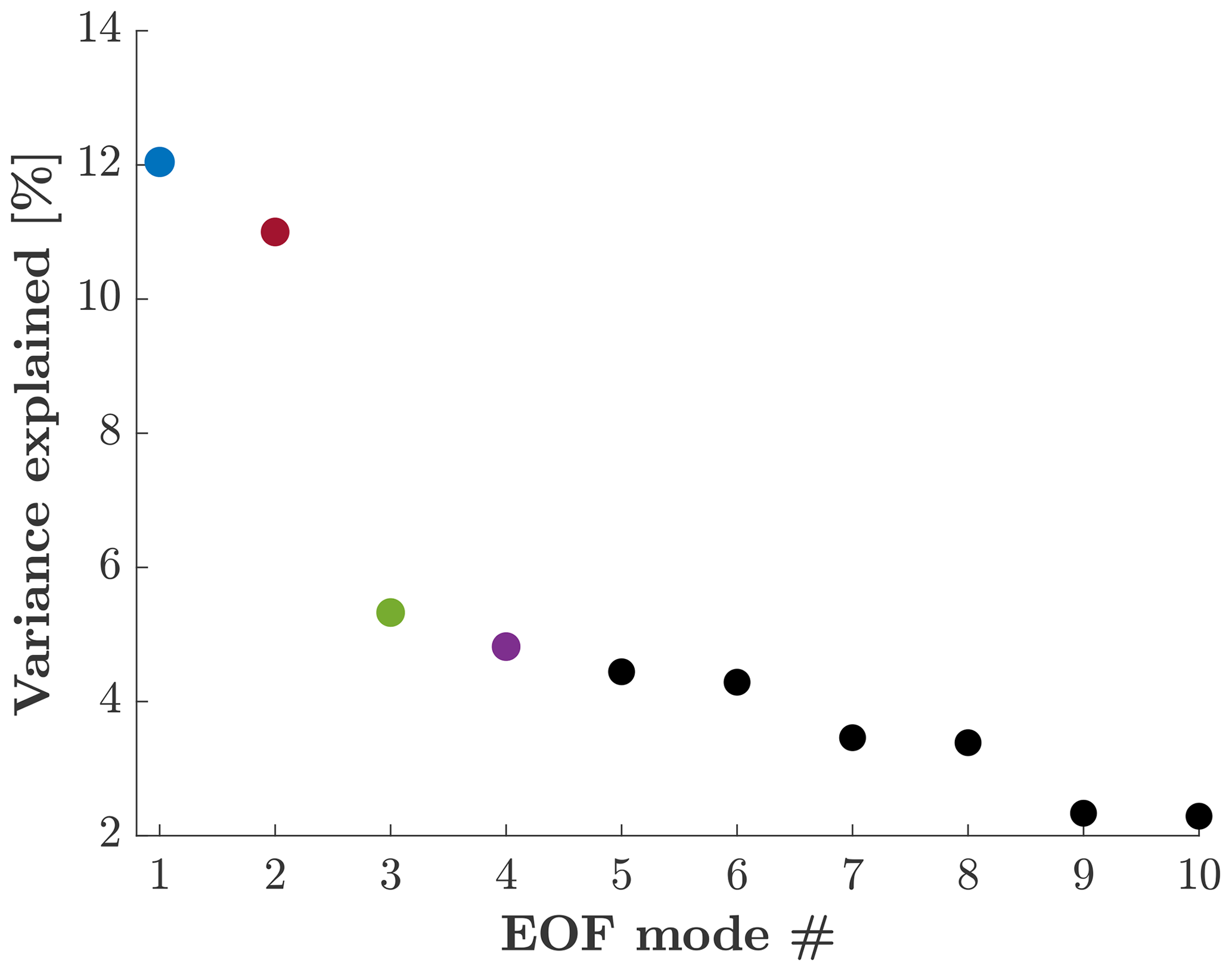
In addition to the spatial structure of the EOF modes, the EOF analysis also yields the percentage of variance explained by each of the modes. The percentage of variance explained by each of the first 10 first EOF modes in a wide channel is shown in Fig. 4. The first four EOFs explain ∼ 33 % of the variance, while any mode higher than 10 accounts for less than ∼ 1 % of the variance.

Figure 4 The variance explained by each of the first 10 EOFs in a wide channel.

The solid lines in Fig. 5 show the fast Fourier transform (FFT) of the first four principal components (PCs) obtained from the EOF analysis. The dashed vertical lines indicate the frequencies of the trapped-waves theory, Eq. (22), with k=0 for n=3, 4, 6, and 9. The dotted vertical lines indicate the frequencies of the harmonic-wave theory, Eq. (18a), for the same modes. As expected, the frequencies obtained from the FFT are much closer to the frequencies of trapped waves than to the frequencies of harmonic waves. Note that the dashed red lines and dotted red lines overlap.

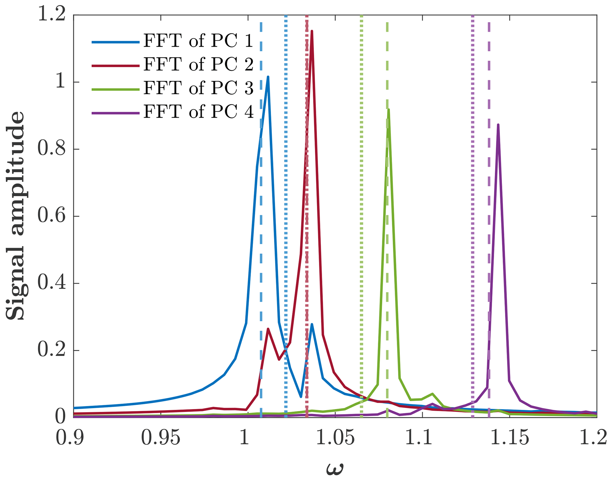
Figure 5 Solid lines show the FFT of the first four PCs in a wide channel. Dashed lines show the trapped-wave frequencies. Dotted lines show the harmonic-wave frequencies.

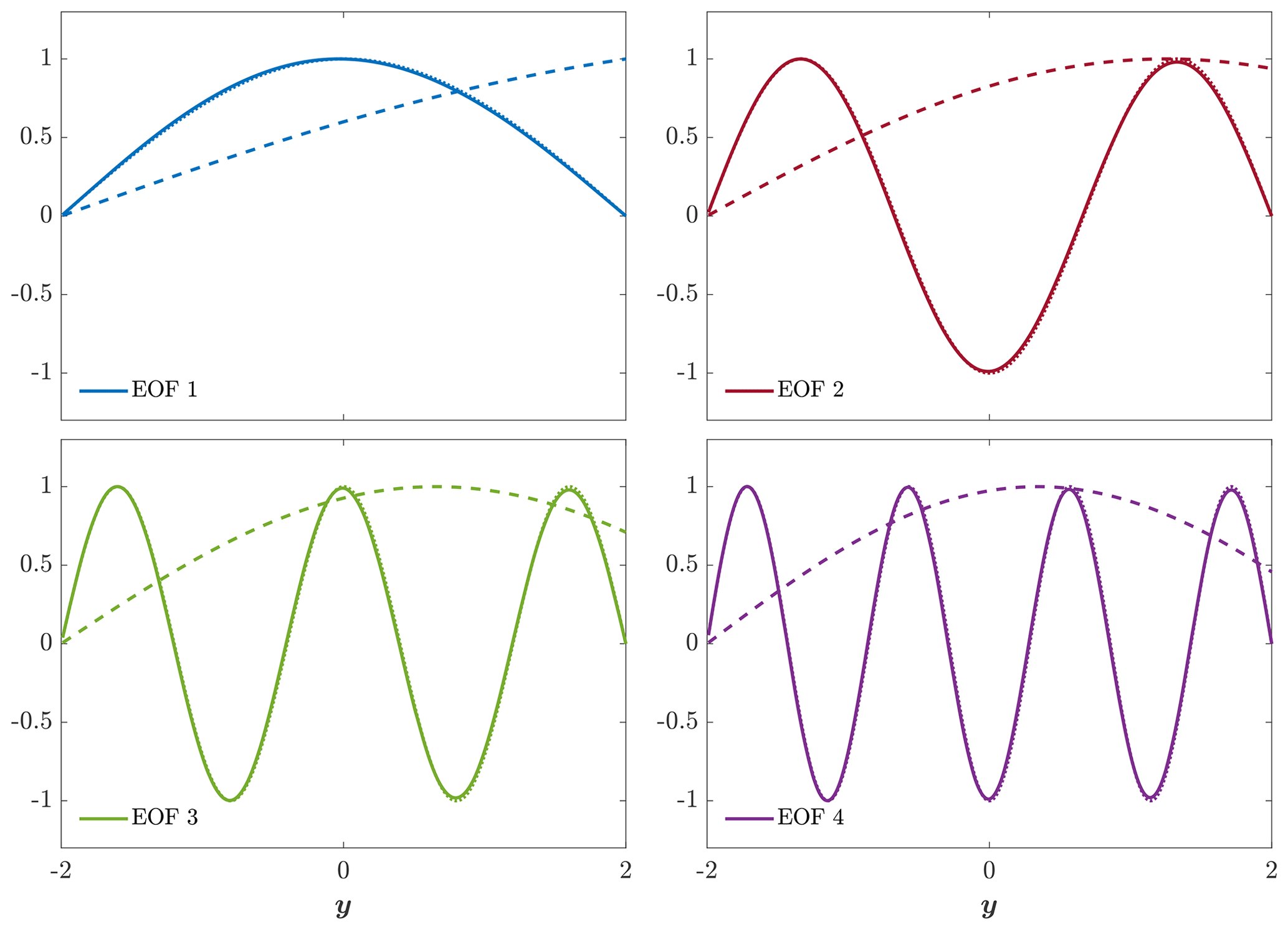
Figure 6 Solid lines show the first four EOFs of v(y,t) in a narrow channel. Dashed lines show the Airy eigenfunctions for n=0 (blue), n=2 (red), n=4 (green), and n=6 (purple). Dotted lines (indistinguishable from the solid lines) show the harmonic eigenfunctions for the same modes. In contrast to a wide channel, in a narrow channel, the EOFs are identical to the harmonic eigenfunctions.

Figures 6–8 show the counterparts of Figs. 3–5 but for a narrow channel, where L_y=4 (and b=0.005 in a wide channel). Figure 6 shows that the first four EOFs of v(y,t) (solid lines) are identical to the harmonic eigenfunctions, Eq. (16), with n=0, 2, 4, and 6 (dotted lines that overlap the solid lines). Clearly, the Airy eigenfunctions, shown by the dashed lines in Fig. 6, are irrelevant for the calculated eigenfunctions in a narrow channel. Figure 7 shows that over 96 % of the variability is explained by the first three EOFs, which should be compared with a wide channel, where the first three modes explain less than 30 % of the variability. We speculate that the EOF algorithm decomposes a signal more efficiently when the basis functions are harmonic. Figure 8 shows that the frequencies obtained from the FFT (solid lines) match those of harmonic modes (Eq. 18a with k=0) very well (dotted lines), while those of the trapped modes (Eq. 22 with k=0) provide extremely poor estimates in a narrow channel (the four dashed vertical lines at ω slightly above 1).

Figure 7 The variance explained by each of the first 10 EOFs in a narrow channel.

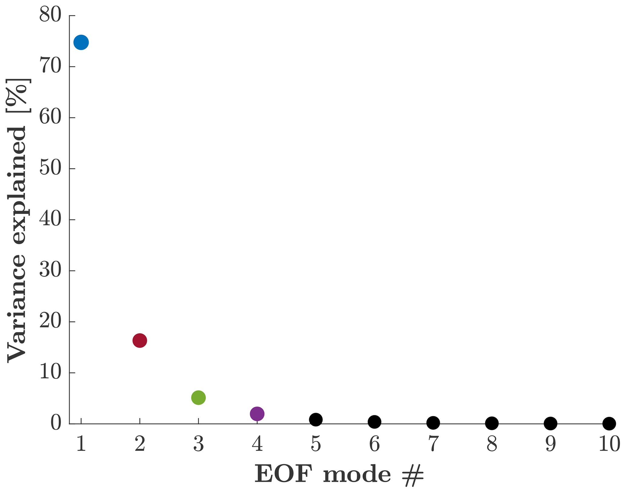
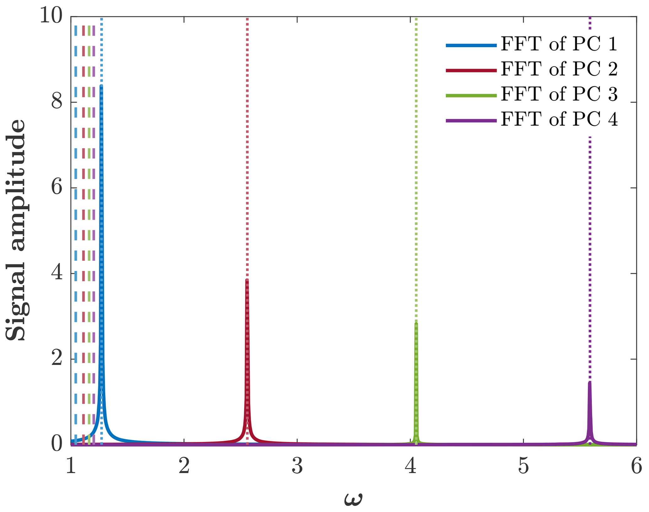
Figure 8 Solid lines show the FFT of the first four PCs in a narrow channel. Dashed lines show the trapped-wave frequencies. Dotted lines show the harmonic-wave frequencies.

5 Two-dimensional adjustment problem

Here we examine the adjustment problem in zonal channels, when η₀(x) is given by Eq. (11). Although η₀ depends only on x, the solution in this case is a function of both x and y, since both the boundary conditions (Eq. 8) and the Coriolis parameter (i.e., the term (1+by) in Eqs. 4–5) depend on y. Thus, the solutions in this case vary with x and y.

5.1 The quasi-geostrophic state

When $\frac{\partial }{\partial x}\ne \mathrm{0}$ the dependence of the meridional variation in the Coriolis parameter generates Rossby waves. The frequency of Rossby waves is distinct from that of Poincaré and Kelvin waves, which causes the adjustment process to take place in two stages. In the first, relatively rapid stage (t=𝒪(10)), the Poincaré and Kelvin waves propagate away from the initial disturbance, leaving a quasi-geostrophic state behind them. This stage resembles the geostrophic adjustment on the f plane. In the second stage, Rossby waves induce a slow westward motion of the initial disturbance and slowly deform the near-geostrophic equilibrium established in the first stage (Blumen, 1972; Gill, 1982, Sect. 11.11). Our simulations show that the second stage itself can be divided into two sub-stages, where in the first sub-stage the near-geostrophic state only drifts westward, while its spatial structure is hardy changed, while in the second sub-stage, wave dispersion becomes dominant, which alters the near-geostrophic state.

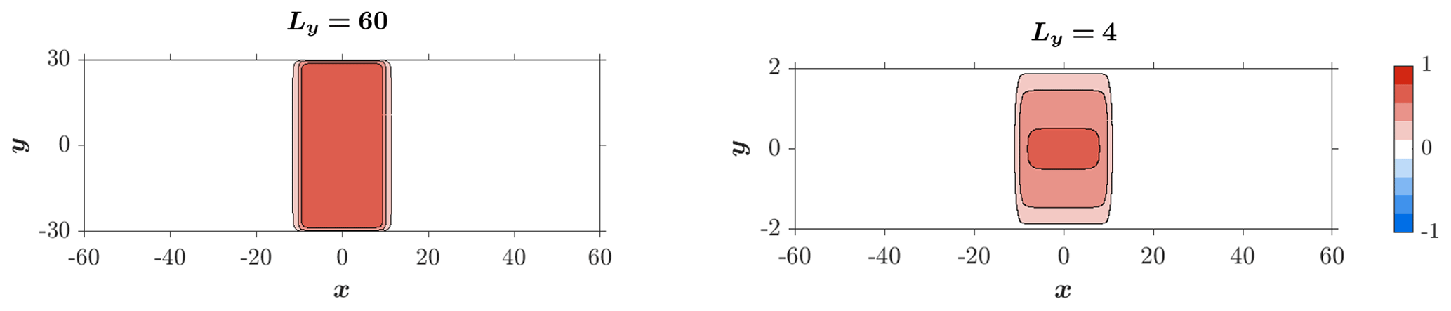
Figure 9 The geostrophic steady state on the f plane in wide and narrow channels. Note the vastly different scales of the ordinates in the two panels.

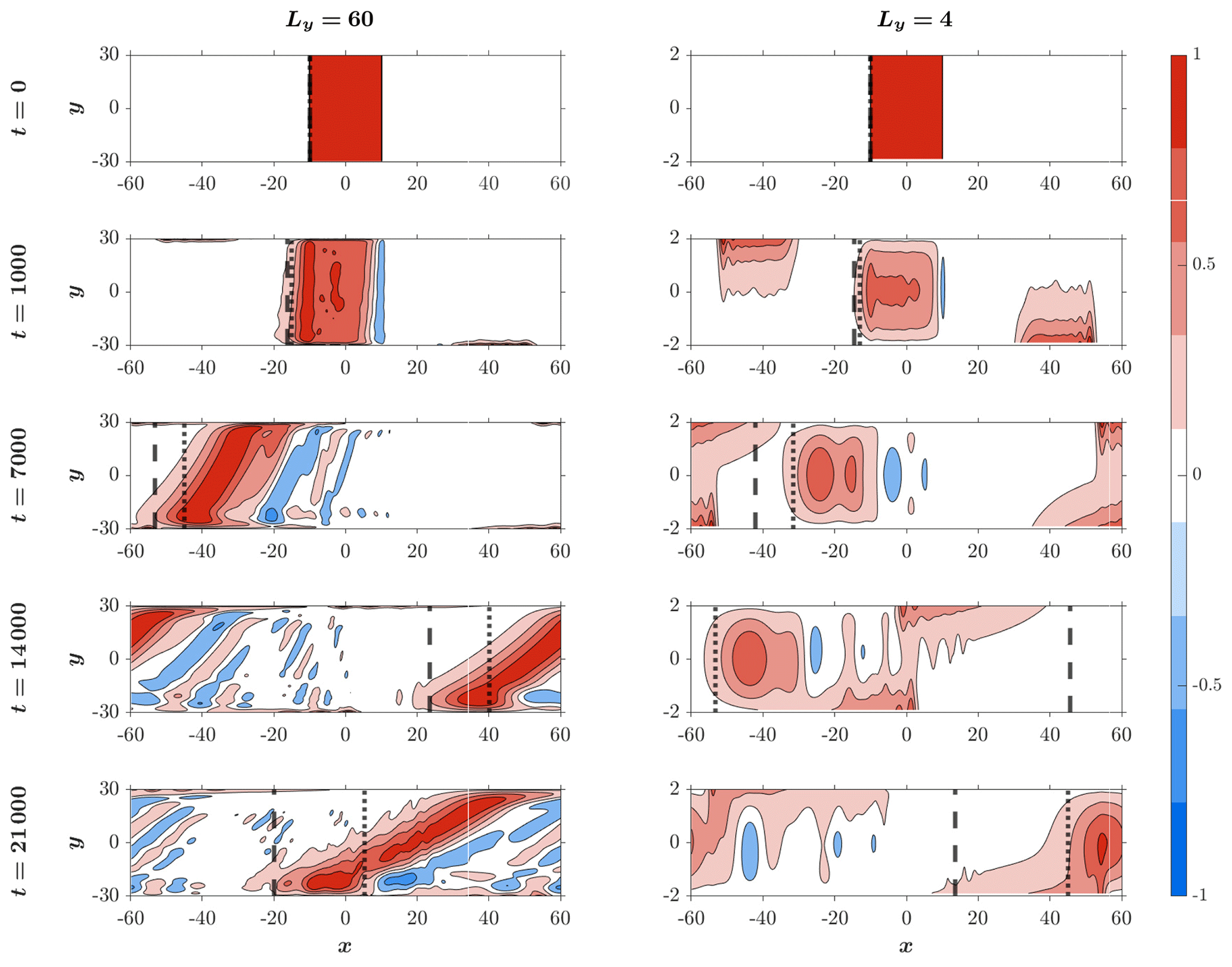
Figure 10 The temporal development of η in wide and narrow channels. Note the emergence of Kelvin waves near the channel walls (most prominent in the narrow channel at t=1000). The near-geostrophic state is shifted westward at the speed of Rossby waves (harmonic in a narrow channel and trapped in a wide channel). The effect of dispersion increases with time. The vertical lines show the location of the leading edge based on the harmonic-wave theory (dotted lines; Eq. 39) and based on the trapped-wave theory (dashed lines; Eq. 40). As expected, the harmonic-wave theory yields more accurate estimates in a narrow channel, while the trapped-wave theory does so in a wide channel.

Figure 9 shows the geostrophic steady state on the f plane (b=0) in wide (L_y=60; left column) and narrow (L_y=4; right column) channels. The steady solutions were calculated using the analytic expressions developed in subsection 5 of the Appendix in Yacoby et al. (2021) for long channels (L_x≫D). In both channels, the steady solutions vary with y only near the boundaries, so their variation with y is less pronounced in wide channels, as the solution there remains (nearly) independent of y throughout most of the channel width (though the width of the boundary layer near the wall is not identical in the two channels; in a wide channel, η is nearly uniform over the $-\mathrm{25}<y<\mathrm{25}$ range). The steady state on the f plane can be compared to the quasi-geostrophic state (i.e., the westward-propagating near-steady state) on the β plane illustrated in Fig. 10.

The temporal development of η on the β plane (b=0.005) in wide and narrow channels was simulated with L_x=120, so $D=L_x/\mathrm{12}$ in Eq. (11) was set to 10 (simulation C). The second row in Fig. 10 shows the westward propagation of the initial disturbance at t=1000 (∼10² d). During this (short) time, the effect of wave dispersion is relatively small, and the initial state only shifts westward by ≈15R_d, while adjusting to a near-geostrophic state (close to that shown in Fig. 9). Kelvin waves are also evident at this time near the meridional boundaries. In contrast, for t≥7000 (third to fifth rows in Fig. 10), the massive deformation due to wave dispersion is evident in the simulations. The simulations also highlight the fact that wave dispersion is more significant in a wide channel than in a narrow channel.

The speed of westward migration, i.e., the speed of the leading edge, c_max, can be estimated from the phase speeds of long harmonic and trapped Rossby waves (i.e., by substituting $n=\mathrm{0}=k$ in the dispersion relations). For harmonic waves, Eq. (18b) implies

$$\begin{array}{}\text{(39)}& c_{max}={\displaystyle \frac{-b}{\mathrm{1}+{\mathit{\pi }}^{\mathrm{2}}/L_y^{\mathrm{2}}}},\end{array}$$

while for trapped Rossby waves, Eq. (23) implies

$$\begin{array}{}\text{(40)}& c_{max}={\displaystyle \frac{-b}{\mathrm{1}+(\mathrm{2}b{)}^{\mathrm{2}/\mathrm{3}}{\mathit{\xi }}_{\mathrm{0}}-b{L}_y}}.\end{array}$$

The dotted vertical lines and dashed vertical lines in Fig. 10 indicate the position of the leading edge using Eqs. (39) and (40), respectively. Clearly, in a narrow channel, the leading edge moves with the speed of a harmonic Rossby wave, while in a wide channel it moves with the speed of a trapped Rossby wave. A comparison between the η fields in the two channels at t = 21 000 (fifth row) shows that in a narrow channel the field resembles the f plane steady state shown in Fig. 9 much more closely than in a wide channel (i.e., the wave dispersion distorts the field more efficiently in a wide channel than in a narrow one).

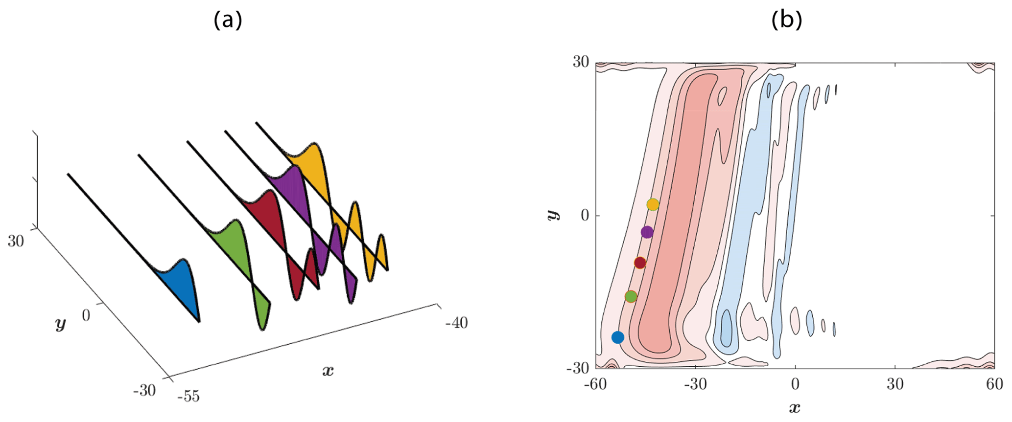
Figure 11 Dispersion of the Airy trapped waves in a wide channel. (a) Meridional structure of the first five trapped-wave modes (n=0, 1, 2, 3, 4) at t=7000. The locations of the wave modes were calculated from the phase speed of trapped Rossby waves, with k=0 (i.e., Eq. 41). The lower the wave mode, the faster the phase speed. As a result, the southern part of the wavefront moves faster than the northern part, since low modes occupy only the former. (b) Colored dots are the locations of the peaks of the Airy wave modes shown in panel (a) at t=7000. The contours are η at t=7000 (as in the third panel from the top in the left column of Fig. 10). The locations of the peaks are consistent with the numerical results (contours) and explain the slope in the wavefront.

From the left column of Fig. 10, it is evident that in a wide channel, where the trapped-wave theory applies, the southern part of the wavefront moves faster than the northern part, causing a latitudinal tilting of the wavefront that increases with time. This phenomenon was established in prior numerical simulations of the β plane (e.g., Sura et al., 2000, and Isachsen et al., 2007). The latitudinal tilting was heuristically attributed in these studies to the decrease with latitude of the Rossby wave phase. Clearly, the harmonic-wave theory cannot explain the latitudinal tilting, since all long waves propagate at the same phase speed. In the alternate, trapped-wave theory, the tilt of the wavefront is easily explained by the dispersion of the non-harmonic waves. In this theory, the phase speed of trapped Rossby waves with k=0 is as follows:

$$\begin{array}{}\text{(41)}& c_{\mathrm{ph}}={\displaystyle \frac{-b}{\mathrm{1}+(\mathrm{2}b{)}^{\mathrm{2}/\mathrm{3}}{\mathit{\xi }}_n-b{L}_y}},\end{array}$$

which decreases with ξ_n; i.e., the lower the wave mode, the faster the phase speed. Also, for higher wave modes, the domain where the trapped wave oscillates and does not decay extends farther away from the channel's southern boundary, causing the wave peak to shift further northward. As a result, the southern part of the wavefront (where the low modes have O(1) amplitude) moves faster than the northern part, which is dominated by high modes. This mechanism is illustrated in Fig. 11, where the sub-range in the channel in which the amplitude of a particular mode is O(1) is shown in Fig. 11a, and the distance traveled by that mode in 7000 time units is shown in Fig. 11b as a dot overlaid on the η contours of the t=7000 panel in the left column in Fig. 10.

The temporal development of η in narrow channels on the β plane (right column of Fig. 10) can be compared to the development of η on the f plane illustrated in Fig. 8 of Yacoby et al. (2021). Note that the simulation time in the latter is much shorter than here.

5.2 Rossby waves

As was done in the one-dimensional case studied in Sect. 4.3, we also use the EOF method to examine the spatial and temporal structures of the waves in the two-dimensional case. The analyses are performed on $v(x=-\mathrm{50},y,t)$, as calculated by the MITgcm (simulation D).

Figure 12 shows the results of the analysis in a wide channel. The solid lines in Fig. 12a–b show the first two EOFs of $v(x=-\mathrm{50},y,t)$. The dashed lines show the Airy eigenfunctions, Eq. (20), for n=0 (blue) and n=2 (red). The dotted lines show the harmonic eigenfunctions, Eq. (16), for the same wave modes. All curves are normalized using the normalization employed in Figs. 3 and 6. Similar to the results in the one-dimensional problem, in a wide channel, the EOFs have the same structure as the Airy eigenfunctions. However, in the two-dimensional case, the differences between the EOF modes and the corresponding Airy eigenfunctions are more substantial than in the one-dimensional case (Fig. 3). We hypothesize that some of the differences between the EOFs and the eigenfunctions result from a relatively low spatial and temporal resolution of simulation D (compared to simulation B; see Table 1). Clearly, the structures of the harmonic modes approximate those of the EOF modes very poorly. Figure 12c shows the variance explained by each of the first 10 EOF modes. The first two EOFs explain 47 % of the variance. The solid lines in Fig. 12d–e show the FFT of the first (blue) and second (red) PCs. The vertical blue dashed lines and vertical red dashed lines show the frequencies of the n=0 and the n=2 trapped modes (respectively) given by Eq. (23), where $k=\mathit{\pi }(m+\mathrm{1})/L_x$ for m=1, 3, 5, and 7. The vertical blue dotted lines and vertical red dotted lines show the harmonic frequencies given by Eq. (18b) for the same wave modes. Clearly, the frequencies obtained from the FFT are much closer to the trapped-wave frequencies than to the harmonic-wave frequencies.

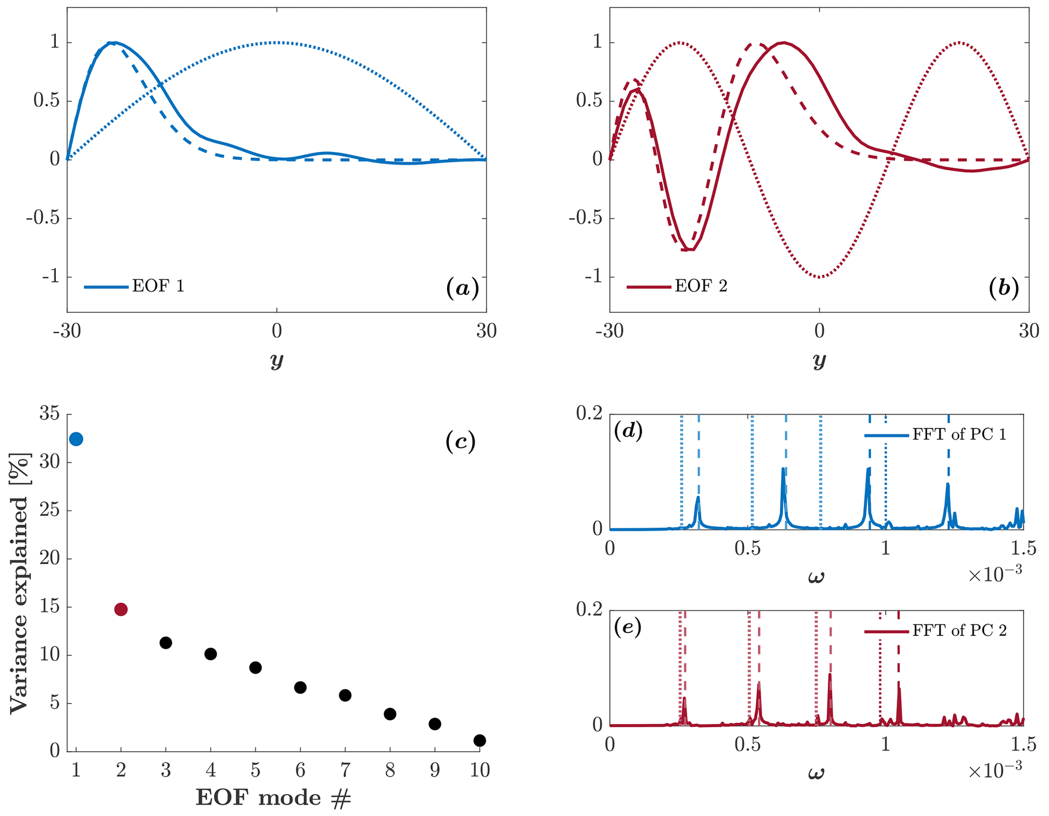
Figure 12 EOF analysis of Rossby waves in a wide channel. (a–b) Solid lines show the first two EOFs of $v(x=-\mathrm{50},y,t)$, dashed lines show the Airy eigenfunctions for n=0 (blue) and n=2 (red), and dotted lines show the harmonic eigenfunctions for the same modes. (c) The variance explained by each of the first 10 EOFs. (d–e) Solid lines show the FFT of the first two PCs. Dashed lines show the expected frequencies according to the trapped-waves theory (Eq. 23). Dotted lines show the expected frequencies according to the harmonic-waves theory (Eq. 18b).

Figure 13 As in Fig. 12 but in a narrow channel.

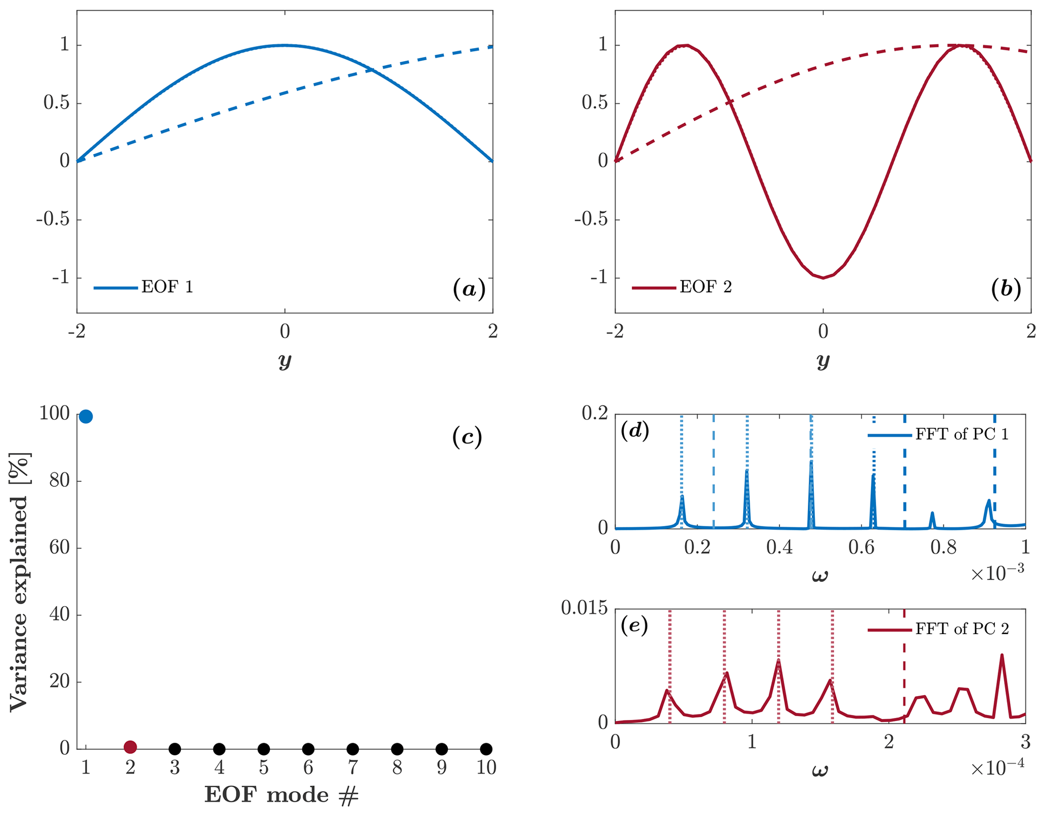
Figure 13 shows the same information as Fig. 12 but for a narrow channel. Figure 13a–b show the first two EOFs that are identical to the harmonic eigenfunctions (Eq. 16) with n=0 and n=2. As in the one-dimensional case, the Airy eigenfunctions provide a very poor approximation to the calculated structure of the EOF modes. Figure 13c shows that the first EOF explains nearly all the variance so that each of the subsequent modes explains a minute fraction of the variance. Figure 13d–e show that the wave spectrum matches the spectrum of harmonic waves. Note that in Fig. 13d the trapped-wave frequencies with m≥3 are outside of the range of the abscissa.

5.3 Poincaré waves

Following the examination of Rossby waves, we turn now to the examination of Poincaré waves. The calculations of the energy evolution, discussed in detail in Sect. 5.4, reveal that the fraction of the initial (potential) energy converted to Poincaré wave energy during the adjustment process decreases with the length of the initial perturbation, 2D. This is consistent with the results found on the f plane in Yacoby et al. (2021). Hence, to increase the energy of Poincaré waves, we decrease the channel length, L_x, to 12 so that $D=L_x/\mathrm{12}=\mathrm{1}$ instead of 10. The EOF analysis is performed on $v(x=\mathrm{5},y,t)$, as calculated by the RSW solver (simulation E).

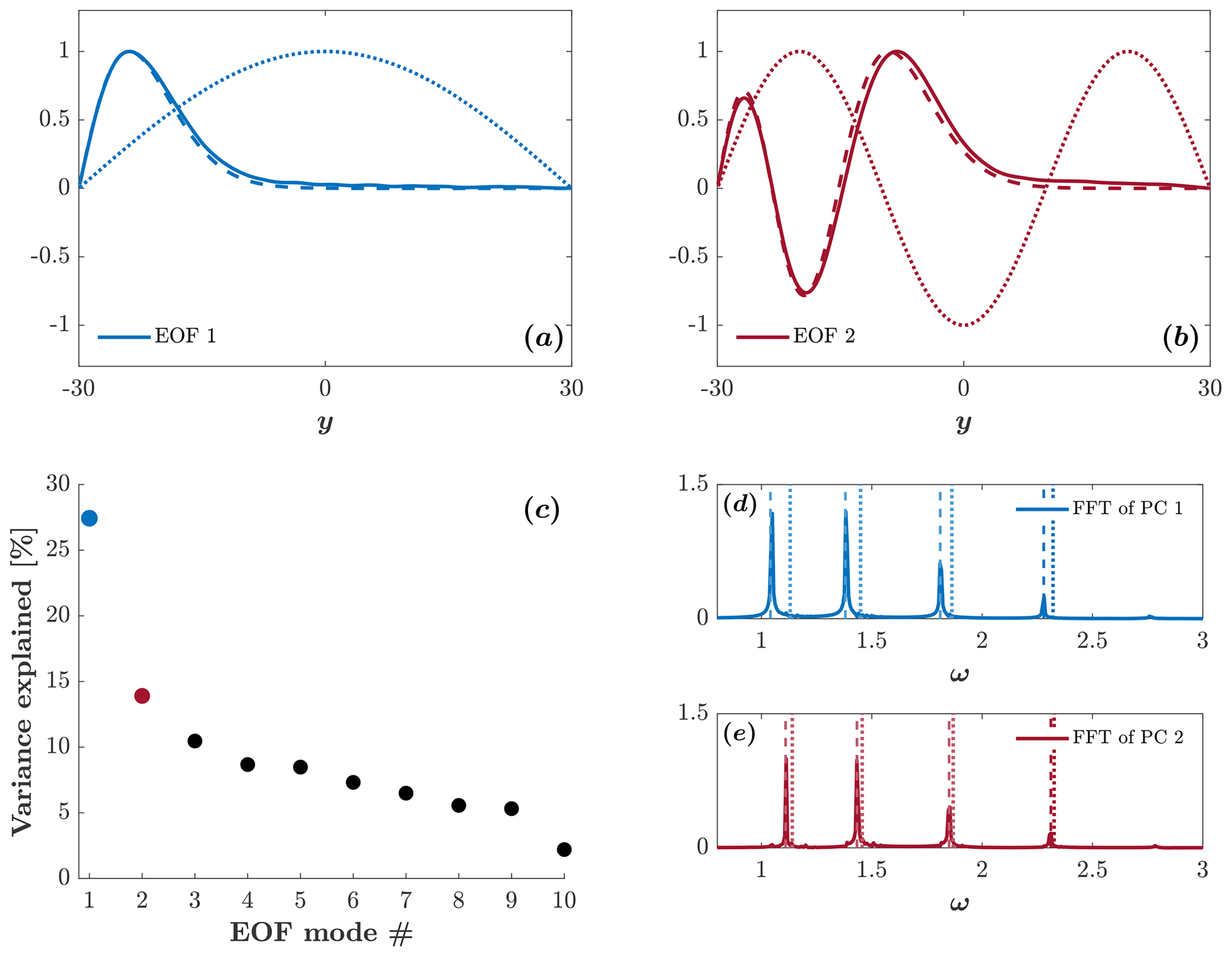
Figure 14 EOF analysis of Poincaré waves in a wide channel. (a–b) Solid lines show the first two EOFs of $v(x=\mathrm{5},y,t)$; dashed lines show the Airy eigenfunctions for n=0 (blue) and n=2 (red); dotted lines show the harmonic eigenfunctions for the same modes. (c) The variance explained by each of the first 10 EOFs. (d–f) Solid lines show the FFT of the first two PCs. Dashed lines show the expected frequencies according to the trapped-waves theory (Eq. 22, where $k=\mathit{\pi }(m+\mathrm{1})/L_x$, with m=1, 3, 5, 7). Dotted lines show the expected frequencies according to the harmonic-waves theory (Eq. 18a for the same wave modes).

The results of the EOF analysis in a wide channel presented in Fig. 14 clearly show that (i) the numerically calculated EOFs of Poincaré waves in Fig. 14a–b are approximated by the Airy eigenfunctions more accurately than by the EOFs of Rossby waves (the latter are shown in Fig. 12a–b); (ii) the first two EOFs shown in Fig. 14c explain ∼40 % of the variance, which is slightly less than the variance explained by the Rossby wave EOFs (the latter are shown in Fig. 12c); and (iii) the wave spectra in Fig. 14d–e match the spectra corresponding to the Airy waves.

Figure 15 As in Fig. 14 but in a narrow channel.

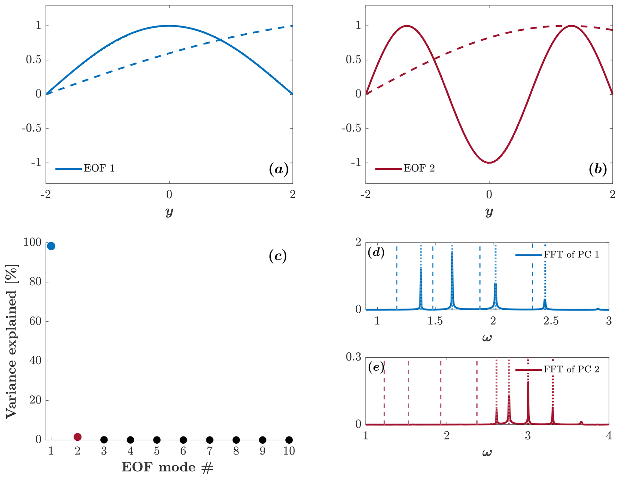
Figure 15 shows the same information as in Fig. 14 but for a narrow channel. The differences between wide and narrow channels, evident from a comparison between the two figures, are such that, in a narrow channel, (i) the first two EOFs are identical to the harmonic eigenfunctions with n=0 (Fig. 15a) and n=2 (Fig. 15b), (ii) the first EOF explains nearly all of the variance (Fig. 15c), and (iii) the wave spectra match the spectra of harmonic waves (Fig. 15d–e).

5.4 Energy

In the previous sections (Sect. 5.1–5.3), we analyzed the results of simulations C, D (L_x=120, D=10), and E (L_x=12, D=1), each with both L_y=4 and L_y=60. In the present subsection, simulations C and E are used to analyze the energy of Rossby waves and establish its relation to the energy of the steady state on the f plane. We prefer simulation C over simulation D because it has a better spatial and temporal resolution. The longer runtime of simulation D was irrelevant here, since we analyzed the energy for t≤1000 only (see Fig. 16). Specifically, we compare the total (potential and kinetic) energy, $\frac{\mathrm{1}}{\mathrm{2}}\left({\mathit{\eta }}^{\mathrm{2}}+u^{\mathrm{2}}+v^{\mathrm{2}}\right)$, of Rossby waves on the β plane to the total (potential and kinetic) energy of the steady state on the f plane. To separate the low-frequency Rossby waves from the high-frequency Poincaré and Kelvin waves, we apply a fifth-order low-pass Butterworth filter (in both forward and reverse directions). The cutoff frequency is set to $\mathit{\omega }=\mathit{\pi }/L_x$ (half the frequency of the Kelvin mode of the lowest frequency, i.e., with $k=\mathrm{2}\mathit{\pi }/L_x$) which separates the frequencies of Rossby waves from the frequencies of Poincaré and Kelvin waves. However, since the integral of the surface initial height distribution,

$$\underset{-L_y/\mathrm{2}}{\overset{L_y/\mathrm{2}}{\int }}\underset{-L_x/\mathrm{2}}{\overset{L_x/\mathrm{2}}{\int }}{\mathit{\eta }}_{\mathrm{0}}\mathrm{d}x\mathrm{d}y=\mathrm{2}D{L}_y,$$

is not 0, Kelvin waves have a mean, time-independent, component (${\stackrel{\mathrm{‾}}{\mathit{\eta }}}_{\mathrm{K}},{\stackrel{\mathrm{‾}}{u}}_{\mathrm{K}}$) in addition to the time-dependent, high-frequency components. For small b, the mean component of Kelvin waves is approximated by

$$\begin{array}{c}{\displaystyle }{\stackrel{\mathrm{‾}}{\mathit{\eta }}}_{\mathrm{K}}={\displaystyle \frac{\mathrm{2}D}{L_x}}\left(e^{-y-L_y/\mathrm{2}}+e^{y-L_y/\mathrm{2}}\right)={\displaystyle \frac{\mathrm{4}D}{L_x}}{e}^{-L_y/\mathrm{2}}\cosh \left(y\right),\\ {\displaystyle }{\stackrel{\mathrm{‾}}{u}}_{\mathrm{K}}=-{\displaystyle \frac{\partial {\stackrel{\mathrm{‾}}{u}}_{\mathrm{K}}}{\partial y}}=-{\displaystyle \frac{\mathrm{4}D}{L_x}}{e}^{-L_y/\mathrm{2}}\sinh \left(y\right).\end{array}$$

To separate the Rossby waves from the time-independent component of the Kelvin waves, we subtract ${\stackrel{\mathrm{‾}}{\mathit{\eta }}}_{\mathrm{K}}$ and ${\stackrel{\mathrm{‾}}{u}}_{\mathrm{K}}$ from η and u after applying the low-pass filter.

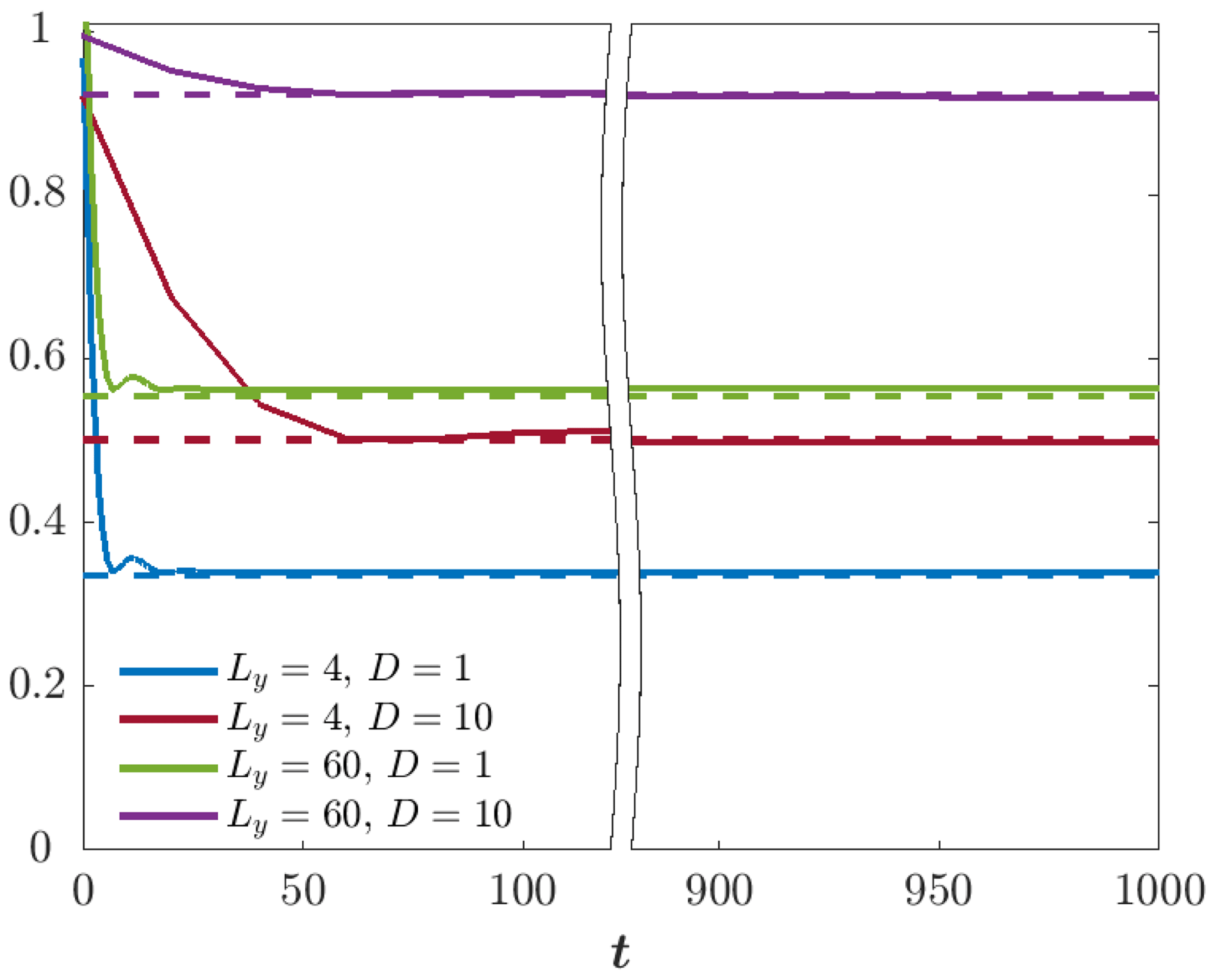
Figure 16 Solid lines show the total (potential and kinetic) energy of Rossby waves as a function of time. Dashed lines show the total energy of the steady state obtained on the f plane. The curves were normalized by the initial energy, L_yD.

The total energy of the steady state obtained on the f plane was calculated using the analytic expressions developed in Sect. 5 of the Appendix in Yacoby et al. (2021) for long channels (see Fig. 9 above). The solid lines in Fig. 16 show the total energy of the Rossby waves (i.e., the integral over the entire channel) as a function of time. The dashed lines show the total energy of the steady state on the f plane. All curves are normalized on the initial energy given by $\frac{\mathrm{1}}{\mathrm{2}}{L}_y{\int }_{-L_x/\mathrm{2}}^{L_x/\mathrm{2}}{\mathit{\eta }}_{\mathrm{0}}(x{)}^{\mathrm{2}}\mathrm{d}x=L_{y}D$. The figure shows that within a relatively brief time (t≈10, when D=1, and t≈60, when D=10), the energy of the Rossby waves reaches the final value that equals the energy of the steady state on the f plane. We hypothesize that the difference in the time it takes the energy of Rossby waves to its final value for D=1 (simulation E) and D=10 (simulation C) is partially due to the difference in the temporal resolution between simulation E ($\mathrm{\Delta }t={\mathrm{10}}^{-\mathrm{3}}$) and simulation C ($\mathrm{\Delta }t={\mathrm{10}}^{-\mathrm{1}}$). The results shown in Fig. 16 affirm that Rossby waves on the β plane are the counterpart of the steady state on the f plane. For given L_y, the initial energy that transforms to Rossby (Poincaré) wave energy increases (decreases) with D.

6 Discussion and summary

This paper examines the process of geostrophic adjustment in periodic zonal channels on the β plane, focusing on the effect of β on the (i) geostrophic steady state, (ii) waves' structure and spectrum, and (iii) energetics of the adjustment process (i.e., the energy conversion ratio, γ, and the energy of Rossby waves). The three issues are addressed in the three following subsections, namely Sect. 6.1–6.3. Each subsection begins with a brief summary followed by a discussion.

6.1 The effect of β on the geostrophic steady state

In the one-dimensional case, the step in η₀(y) given by Eq. (10) parallels the domain's zonal walls (i.e., parallels the x axis). Thus, Poincaré waves propagate in the meridional direction, and upon reaching the zonal walls, they are reflected back into the interior of the channel. Since the reflection takes place in both walls, Poincaré waves never leave the domain, so the geostrophic state shown in Fig. 1 only represents the time-averaged solution over many wave periods and not a steady state that is actually reached by the system at long times. As was shown in Fig. 1, the effect of β on the geostrophic steady state is minor, and its contribution is negligible for b values that are typical of the ocean (b=0.005; first row of Fig. 1) and atmosphere (b=0.05; second row of Fig. 1). The independence of the steady state on β even for b=0.05 and L_y=60 is surprising since, for these values, $b{L}_y/\mathrm{2}=\mathrm{1.5}>\mathrm{1}$ (i.e., the βy term exceeds f₀). Based on the calculations of the steady state in Fig. 1, we suggest that the β effect should be quantified based on the (nearly exponential) distribution of u_g(y) instead of the value of bL_y. According to this argument, the β effect is significant only when the Coriolis frequency, 1+by, vanishes not too far from the center of the channel (i.e., at $y>-\mathrm{2}$). Contrary to the naive approach based on a power series expansion of f(y) near y=0, the deviation of 1+by from 1 does not affect the steady state. Our results suggest that the condition guaranteeing the significance of the β effect = $\mathrm{4}+{\mathrm{2}}^{\prime }q$ is not $b{L}_y/\mathrm{2}\sim \mathrm{1}$ but

$$\mathrm{1}+by\le \mathrm{0}\mathrm{at}y=-\mathrm{2},$$

such that b≥0.5 irrespective of the value of $max\left(y\right)=L_y/\mathrm{2}$. The significant effect of β near the Equator is demonstrated in Killworth (1991) on the equatorial β plane and in Paldor and Dritschel (2021) on a sphere. In contrast, if the Coriolis parameter vanishes far from the center of the channel, i.e., at $y\le -\mathrm{2}$, then the effect of β on the steady state is insignificant. The reason for this is, of course, that at $y\le -\mathrm{2}$ the velocity, u_g, and with it the Coriolis force (i.e. fu_g) are tiny, according to Fig. 1.

In contrast to the one-dimensional case, in the two-dimensional case, the effect of β on the geostrophic state is significant also for b=0.005 and also in narrow channels (L_y=4). The effect originates from the formation of Rossby waves instead of the steady state and the slow westward translation of the quasi-geostrophic state by these waves. As time passes, the dispersion of Rossby waves increases, which alters the structure of the quasi-geostrophic state, as shown in Fig. 10. As is evident in Figs. 10 and 11, in wide channels, the dispersion is more pronounced and causes a latitudinal tilting of the front that increases with time.

6.2 The effect of β on the waves

For b=0.005, we found that harmonic waves provide an accurate approximation for the waves in narrow channels, while trapped waves provide an accurate approximation in wide channels, which agrees with the conclusion of Paldor and Sigalov (2008) and Gildor et al. (2016). Thus, the effect of β on the spectrum and structure of the waves is significant in wide channels, even for small b. However, the definitions of “wide” and “narrow” in this context have to be clarified. The transition from a narrow channel to a wide channel occurs when the condition (Eq. 24) on Ł_y is satisfied, which indicates that the definitions of “narrow” and “wide” are not absolute but depend on (i) the wave mode, n; (ii) the value of b; and (iii)​​​​​​​ the value of Z^∗ (the threshold value that $z\left(y=+\frac{L}{\mathrm{2}}\right)$ has to exceed for $\widehat{v}$ to satisfy the boundary condition at $y=L/\mathrm{2}$) that should be sufficiently large. The discussion of Eq. (38) is based on the choice of $Z^{\ast }=\mathrm{2}$. Thus, substituting $Z^{\ast }=\mathrm{2}$, b=0.005, and ${\mathit{\xi }}_n={\mathit{\xi }}_{\mathrm{0}}=\mathrm{2.338}$ implies that the condition for a channel to be wide is L_y>20.136 (i.e., about 20 deformation radii or about 600 km for R_d=30 km). Furthermore, for higher wave modes, the channel has to be even wider in order to satisfy this condition. These arguments justify our choice of L_y=4 as an example of a narrow channel. On the other hand, L_y=60 satisfies the condition (Eq. 24) even for ${\mathit{\xi }}_n={\mathit{\xi }}_{\mathrm{6}}=\mathrm{10.040}$, which justifies our choice of L_y=60 as an example of a wide channel.

It is worth noting that the satisfaction of the condition (Eq. 24) guarantees that the trapped-wave theory will provide an accurate approximation, but the violation of this condition does not imply that the harmonic-wave theory provides an accurate approximation. An example in which the condition (Eq. 24) is not satisfied and neither the harmonic-wave theory nor the trapped-wave theory provides an acceptable approximation is shown in the lower-right panel of Fig. 3, as EOF 4 (solid purple line) does not perfectly match either the harmonic (dotted purple line) or the Airy eigenfunction (dashed purple line). Nevertheless, it resembles the Airy eigenfunction better than the harmonic eigenfunction.

To conclude the discussion in this subsection, we note that our examination of the waves focuses on the meridional velocity, v, since this variable satisfies the boundary conditions (Eq. 8), so the eigenvalue equation (Eq. 12) is derived for this variable. Thus, the effect of β on Kelvin waves is ignored here, which is justified by the results reported in Paldor et al. (2007), who showed that in Kelvin waves the effect of β is negligible.

6.3 The effect of β on the energy

In the one-dimensional case, Fig. 2 shows that the energy conversion ratio, γ, varies by no more than 10 % when b increases from 0 to 1. This near-independence of γ (that depends only on the initial state, PE₀, and the geostrophic state, KE_g and PE_g) on β reflects the near-independence of the steady state on b (see Fig. 1). As discussed in Sect. 6.1, the effect of β on the steady state is significant only near the Equator (where $b\propto \cos \left({\mathit{\varphi }}_{\mathrm{0}}\right)/{\sin }^{\mathrm{2}}\left({\mathit{\varphi }}_{\mathrm{0}}\right)$ is large). As a result, near the Equator, γ(b) is significantly different from γ(b=0), which is the value of γ on the f plane (results not shown).

In the two-dimensional case, we found that the zonal kinetic energy of Rossby waves (on the β plane) is similar to the zonal kinetic energy of the steady state on the f plane. This implies that the amount of initial energy that transforms into energy of the (high-frequency) Poincaré and Kelvin waves is nearly unaffected by β.

6.4 Additional initial and boundary conditions

The analysis presented above is limited to two initial height distributions, given by Eqs. (10) and (11). While the transition from the trapped-wave theory (in wide channels) to the harmonic-wave theory (in narrow channels) is probably relevant to all initial conditions, some of the results presented above are expected to vary with the initial conditions, e.g., the distribution of energy between the different wave types (Rossby, Poincarè, and Kelvin), the structure of the dominant EOFs, and the variance explained by each of them. The present analysis is also limited to zonal periodic channels, while other boundary conditions such as the introduction of meridional walls (i.e., a rectangular basin) require further analysis. A complete description of the geostrophic adjustment on the β plane has to address the adjustment process under different initial and boundary conditions, and this study is a first attempt in this direction.

6.5 Ocean response to a sudden wind stress

This study examines the adjustment process of an initially unbalanced ocean, where the waves are driven by an initial height disturbance. While progress on extending this particular problem to the midlatitude β plane has been limited, other ocean adjustment problems have been extensively studied on the β plane in recent decades. An example of such an ocean adjustment problem is the ocean's response to a wind stress impulse that generates westward-moving Rossby waves that cause a thinning of the western boundary layer (see, e.g., Anderson and Gill, 1975). The applicability of the trapped-waves theory to the wind-driven adjustment problem remains uncertain. Nonetheless, simulations of the forced LRSWEs with no x variations, i.e., Eqs. (25)–(27) with wind forcing, suggest that trapped waves are indeed generated in this adjustment scenario (results not shown). Furthermore, the slope in the Rossby wavefront observed in the two-dimensional wind-driven adjustment problem (see, e.g., Sura et al., 2000) agrees with the slope shown in Fig. 11, which was attributed to the dispersion of trapped waves but does not occur in harmonic waves.

6.6 Nonlinear effects

This study focuses on the linear theory on the β plane. We note that the nonlinear geostrophic adjustment on the f plane is similar to the linear adjustment on the β plane in that both occur in two stages. In the present study, this is demonstrated in Sect. 5.1. In the nonlinear adjustment on the f plane, this was pointed out in Gill (1976, Sect. 9), Hermann et al. (1989), Tomasson and Melville (1992), and Reznik et al. (2001). In the rapid first stage, the evolution is determined by the fast Poincaré waves (that exist on both the f plane and the β plane). The second stage is much slower, and the mechanisms that drive it differ between the linear β plane and the nonlinear f plane. While on the linear β plane this stage is driven by Rossby waves, in the nonlinear adjustment on the f plane, this stage is driven by advection of PV. We conclude by noting that Reznik et al. (2001, Sect. 5) remark (but do not develop a complete theory) on the nonlinear geostrophic adjustment on the β plane. This important issue is left for future work.

6.7 Applicability of the trapped-wave theory to the ocean

As with all Sturm–Liouville eigenvalue problems, any particular solution of the eigenvalue equation (Eq. 12) requires boundary conditions. Thus, the properties of all wave solutions are determined by the conditions imposed at the boundaries. However, geographically, no solid meridional boundaries exist at midlatitudes in the Atlantic or Pacific oceans, which stimulates the question about the applicability of any wave theory to the real ocean. Despite the lack of actual meridional boundaries, we estimate that the trapped-wave theory can be applied to the ocean for the following reasons:

• i.

  Several fundamental models of physical oceanography assume solid boundaries, e.g., the Stommel and Munk models of the wind-driven midlatitude gyres (see, e.g., Vallis, 2017, Chap. 19). Nonetheless, their applicability to the ocean is well established (Gianchandani et al., 2021). In fact, all wave theories have to assume either the existence of boundaries or an infinite domain (i.e., L_y→∞). Clearly, the second assumption violates the basic β plane assumption by≪1 (or βy≪f₀ in a dimensional form).

• ii.

  There exist cases in which the velocity field is assumed to be dynamically confined to a specific region, despite the absence of physical bounding walls. An example in which the existence of such a region has to be assumed is the equatorial zone. Indeed, this assumption provides the justification for the Matsuno (1966) model of equatorial waves, where it is assumed that the meridional velocity vanishes at infinity, while the meridional domain is small enough for the first-order expansion of the β plane approximation to be valid.

• iii.

  The amplitude of trapped waves decays toward the pole faster than the exponential. Therefore, the trapped-wave theory requires only a single wall that marks the equatorward boundary of the domain, where the meridional velocity has to vanish. This is in contrast with the harmonic theory that requires two such walls instead of one. While zonal channels do not exist in the midlatitude oceans, a single zonal wall does exist in some particular places. Such a region, in which the trapped-wave theory has been successfully applied, is the Indian Ocean to the south of Australia. This region is sufficiently wide (in the zonal direction) and is bounded on its equatorward side by a nearly zonal coast. Indeed, trapped Rossby waves were observed in the Indian Ocean by satellite-borne altimeters (De-Leon and Paldor, 2017).

• iv.

  Though zonal channels are scarce in the current midlatitude oceans, they may have been more abundant in past geologic periods, e.g., the early Paleogene (∼ 60 million years ago (Ma); see Fig. 1 in Farouk et al., 2014) and the Early Cretaceous (the Barremian age, ∼ 120 Ma; see Fig. S5q in Farnsworth et al., 2019), so the trapped-wave theory may be relevant to paleo-ocean dynamics.