Impact of sea level changes on future wave conditions along the coasts of western Europe

Wind waves and swells are major drivers of coastal environment changes and coastal hazards such as coastal flooding and erosion. Wave characteristics are sensitive to changes in water depth in shallow and intermediate waters. However, wave models used for historical simulations and projections typically do not account for sea level changes whether from tides, storm surges, or long-term sea level rise. In this study, the sensitivity of projected changes in wave characteristics to the sea level changes is investigated along the Atlantic European coastline. For this purpose, a global wave model is dynamically downscaled over the northeastern Atlantic for the 1970–2100 period under the SSP5–8.5 climate change scenario. Twin experiments are performed with or without the inclusion of hourly sea level variations from regional 3D ocean simulations in the regional wave model. The largest impact of sea level changes on waves is located on the wide continental shelf where shallow-water dynamics prevail, especially in macro-tidal areas. For instance, in the Bay of Mont-Saint-Michel in France, due to an average tidal range of 10 m, extreme historical wave heights were found to be up to 1 m higher (+30 %) when sea level variations are included. At the end of the 21st century, extreme significant wave heights are larger by up to +40 % (+60 cm), mainly due to the effect of tides and mean sea level rise. The estimates provided in this study only partially represent the processes responsible for the sea-level–wave non-linear interactions due to model limitations in terms of resolution and the processes included.

1 Introduction

Coastal zones are among the most densely populated and urbanized areas in the world (McMichael et al., 2020; Neumann et al., 2015; Wolff et al., 2020) which implies that monitoring their evolution in the context of climate change is important in several aspects. Wind waves and swells are major drivers of coastal environment changes (Ranasinghe, 2016) and can drive coastal marine hazards such as coastal flooding (Melet et al., 2020b).

To build knowledge on future changes in wave climate, a growing number of global and regional wave projections have been developed and intercompared (Hemer et al., 2013; Morim et al., 2018, 2021, 2023; Meucci et al., 2020; Lobeto et al., 2021). These projections are commonly based on dynamical wave models often forced by surface winds projected by climate models contributing to the Coupled Model Intercomparison Project (CMIP), with potential downscaling of atmospheric forcing. A multi-model analysis is required to assess the uncertainties and robustness of projected changes in wave climate. Morim et al. (2018, 2019) provided a review of wave projections. Over the northeastern Atlantic and Mediterranean Sea bordering the coasts of western Europe, models project a robust decrease in annual and seasonal mean significant wave height together with a decrease in the mean wave period. Regarding mean wave direction, a robust clockwise change is projected for the Iberian Atlantic coast. Extreme significant wave heights are also consistently projected to decrease over the northeastern Atlantic and Mediterranean Sea (Morim et al., 2018, 2021; Aarnes et al., 2017).

Wave characteristics are sensitive to changes in water depth and thus to sea level variations in shallow and intermediate waters, where waves start to interact with the ocean bottom. This occurs through a variety of processes. Very close to the coast, in shallow waters, depth-induced wave breaking is the fundamental mechanism, but it is a small-scale process that is often omitted in climate projections due to the coarse resolution of global and regional models. In intermediate waters, at a greater distance from the coast, larger-scale processes can also be affected by sea level variations, for instance through bottom friction effects. At fine spatial scales, wave statistics have already been shown to be sensitive to sea level rise (Chini et al., 2010; Wandres et al., 2017; Arns et al., 2017) and to tides and surges during extreme-wave events (Alari, 2013; Viitak et al., 2016; Fortunato et al., 2017; Idier et al., 2019; Lewis et al., 2019; Staneva et al., 2021; Calvino et al., 2022). However, large-scale wave models used for historical simulations and projections typically do not account for sea level changes, whether from tides, storm surges, or long-term sea level rise. Nevertheless, these wave climate simulations are likely to be influenced by sea level variations through small- to large-scale processes, depending on those included in the model.

The present study aims at investigating the sensitivity of mean and extreme-wave climate conditions to the sea level changes. To that aim, regional historical simulations and projections of waves are produced over the 1970–2100 period considering the high-emission, low-mitigation (SSP5–8.5) climate change scenario (O'Neill et al., 2016). The simulations are produced over the northeastern Atlantic region, called the IBI domain (Iberia–Biscay–Ireland). To assess the sensitivity of wave characteristics to sea level changes, the regional wave model is adapted to consider hourly variations of sea level from a 3D regional ocean model described in Chaigneau et al. (2022).

The paper is organized as follows. The wave model and regional wave simulations are presented in Sect. 2. Simulated mean and extreme wave conditions are compared to observations over the historical period and to previously published 21st century projections in Sect. 3. Section 4 provides an assessment of the sensitivity of wave characteristics to the sea level changes along the European Atlantic coastlines. Finally, results are discussed in Sect. 5, and conclusions are drawn in Sect. 6.

2 Methods: models and simulations

Two regional wave configurations IBI-CCS-WAV (Iberia–Biscay–Ireland Climate Change Scenarios WAVe) (Sect. 2.2) and IBI-CCS-WAV_ssh (Sect. 2.3) are set up to dynamically downscale global wave simulations over the IBI domain considering or not considering hourly sea level outputs as a forcing in the wave model (Sect. 2.1). Table 1 summarizes the different simulations used in the study, namely the simulations performed and analyzed in this paper, the simulations used for the forcings, and the simulations used for the validation in Sect. 3. Appendix A describes the downscaling strategy and the links between the different simulations used to force the regional wave model.

Table 1 List of the different wave and ocean simulations used in the study.

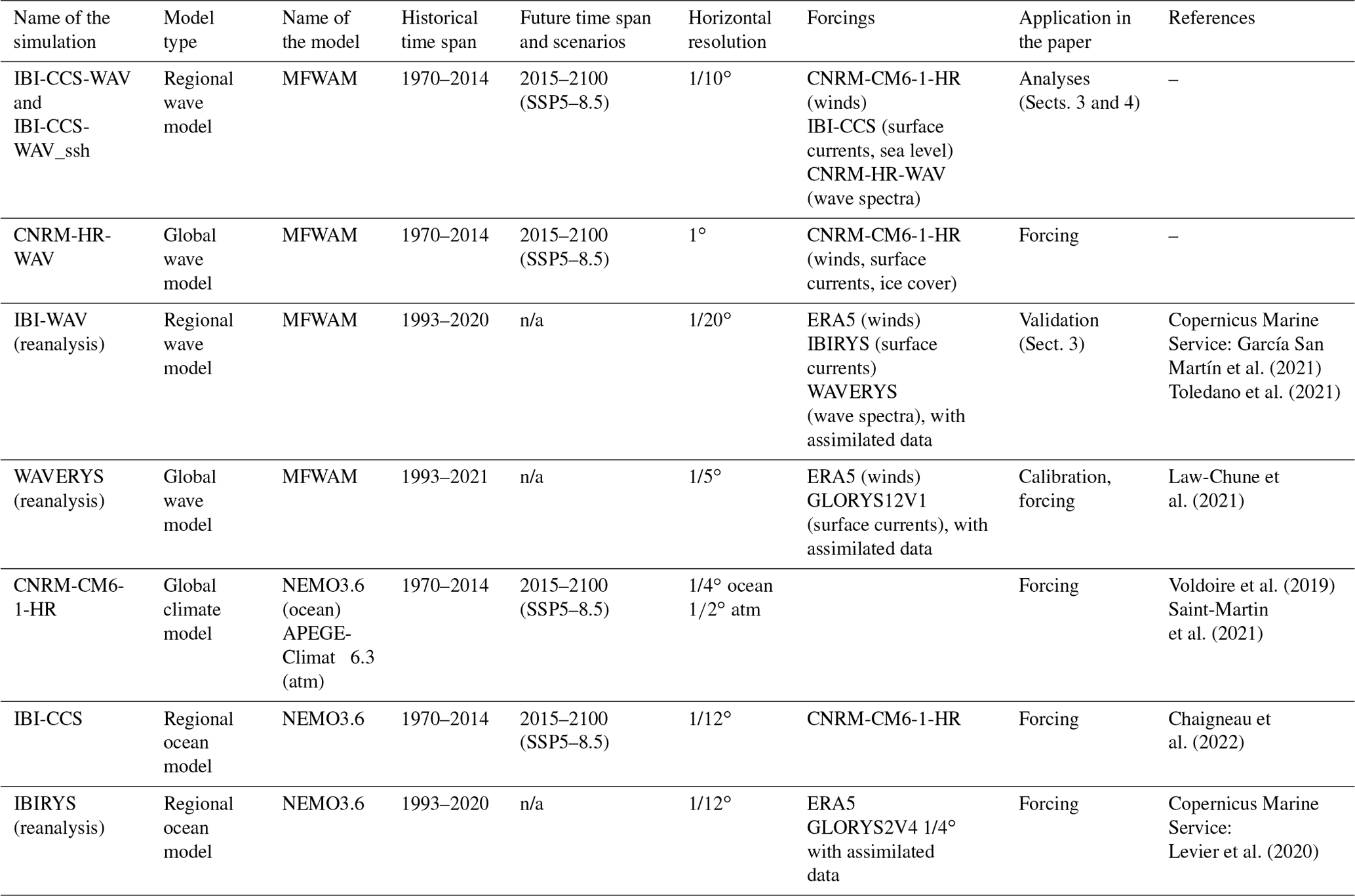
^* n.a – not applicable

2.1 The numerical wave model: MFWAM

The MFWAM (Météo-France WAM) wave model is a spectral sea state prediction model (wind waves and swell). It is a modified version of IFS ECWAM-CY41R2 cycle (ECMWF, 2014) developed at Météo-France for their operational applications (Aouf and Lefèvre, 2015). The variables used to force such a model are surface winds, ocean currents, and sea ice cover, if the latter is relevant for the ocean domain.

Supported by the assimilation of satellite observations, MFWAM is successfully operated within the Copernicus Marine Service (https://marine.copernicus.eu/, last access: 5 July 2024) to provide near-real time (analyses and/or forecasts) and multi-year (reanalysis and/or hindcasts) wave products over both the global ocean and the northeastern Atlantic, corresponding to the region of interest in this study.

MFWAM primarily aims at describing the open-ocean sea states. As such, source terms include physical processes that generate (wave growth by wind according to Bidlot et al., 2007), dissipate (white-capping, dissipation by friction between long and short waves, and bottom friction according to Ardhuin et al., 2010), or redistribute wave energy (non-linear interactions between waves according to Hasselmann et al., 1985), as in Law-Chune et al. (2021). Technical details of the model are explained in Law-Chune et al. (2021). In addition, since we are interested, in this paper, in the coastal shallow-water processes, we additionally include in the model the dissipation due to coastal depth-induced wave breaking with the parametrization of Battjes and Janssen (1978). This choice is in line with other spectral wave models (e.g., Valiente et al., 2023). All the processes included in the model, which occur from the deep ocean to the shallow coastal waters, are likely to be affected by sea level variations.

2.2 Regional wave simulations without sea level variations: IBI-CCS-WAV

The IBI zone is interesting for wave modeling, as it contains a variety of physical processes. First, the domain contains strong variations of bathymetry, with a wide continental shelf in the northern part of the domain (North Sea and English Channel) and a narrow continental shelf in the southern part (Spain, Portugal, Morocco, and Mediterranean Sea) (Fig. 1). There are also contrasting wave regimes: the Atlantic coasts are subject to very energetic events in terms of significant wave heights, wave periods, and energy flows (Masselink et al., 2016; Bruciaferri et al., 2021), whereas the Mediterranean Sea and North Sea are more sheltered areas dominated by wind waves (Chen et al., 2002; Bergsma et al., 2022). In addition, the zone also contains very different tidal regimes with both macro and micro tidal regimes: macro tidal regime in the English Channel and the Celtic Sea (Valiente et al., 2019; Stokes et al., 2021) and micro tidal regime in the Mediterranean Sea.

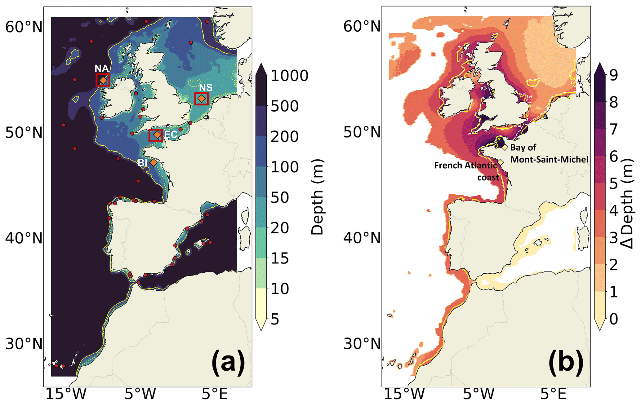
Figure 1 (a) Bathymetry (m) of the IBI domain in the regional wave model. The shelf break (defined by the 200 m isobath) is indicated by the solid yellow line. The dotted yellow lines indicate the areas where the waves start to interact with the bathymetry in IBI-CCS-WAV (intermediate waters that cannot be considered to be purely deep water), identified when $h<L/\mathrm{2}$, with h being the bathymetry and L being the mean wavelength over the 1993–2014 period. The red dots represent the locations of the wave buoys from the Copernicus Marine Service (Wehde et al., 2021) used for the validation in Sect. 3.1. The three red boxes are used in Appendix A to validate extreme winds of the global climate model. Orange diamonds indicate the wave buoys used for the wave rose calculation of Sect. 3.1.2 and 3.2.2 (North Atlantic (NA) buoy 6200093 and Belle-Ile (BI) buoy 6200074) used for the extreme-wind validation in Appendix A (North Atlantic (NA) buoy 6200093, English Channel (EC) buoy 6200103, and North Sea (NS) buoy 6200145). (b) Bathymetric adjustment (Sect. 2.3) that corresponds approximately to the M2 tidal range from the 3D regional ocean model (1993–2014). The lines indicate the areas where the waves start to interact with the bathymetry at low tide (dashed white lines) and at high tide (solid yellow lines). The two yellow diamonds indicate the zones where the impact of including hourly sea level outputs in the wave model is assessed in Sect. 4.

Regional wave simulations IBI-CCS-WAV (IBI Climate Change Scenarios WAVe) are produced using MFWAM (Sect. 2.1) at a $\mathrm{1}/\mathrm{10}$^∘ resolution. The configuration was designed over the IBI domain based on the Copernicus Marine Service regional configuration (Table 1, IBI-WAV, https://doi.org/10.48670/moi-00030). The regional domain covered by IBI-CCS-WAV extends from 27 to 61^∘ N and from 17^∘ W to 8^∘ E (Fig. 1), leading to a horizontal resolution ranging from 5.5 to 10 km. The regional wave configuration is used to dynamically downscale global wave simulations. The dynamical downscaling method allows the resolution of regional processes at a finer scale. The method consists of forcing the regional wave model at its lateral boundaries with wave spectra from the larger-scale wave model and at the surface with winds and surface currents from other suitable models (global climate model and 3D regional ocean model, Table 1). The models and simulations that provide these forcings are described in Appendix A. The bathymetry used is a smoothed ETOPO1 ocean bathymetry (https://sos.noaa.gov/datasets/etopo1-topography-and-bathymetry/, last access: 5 July 2023). The wave simulations are performed over the historical period (1970–2014) and the 21st century (2015–2100) under the SSP5–8.5 climate change scenario. Classical integrated wave parameters such as the significant wave height H_s and the peak period T_P are generated hourly.

2.3 Regional wave simulations with sea level variations: IBI-CCS-WAV_ssh

To measure the impact of sea level changes on waves in the IBI region, a twin configuration to IBI-CCS-WAV (Sect. 2.2) was set up to consider sea level variations as an additional forcing, namely IBI-CCS-WAV_ssh. For this purpose, MFWAM (Sect. 2.1) has been modified to include hourly sea level forcing coming from the same 3D regional ocean simulations as the surface currents. Hourly sea level forcing includes tides, storm surges, and mean sea level but also the non-linear interactions between these processes. In our ocean simulations, the mean sea level contains the sterodynamic sea level (thermal expansion and dynamic sea level associated with ocean circulations) and the barystatic sea level change (the addition of water mass into the ocean); thus, long-term sea level rise over the next century is included in the hourly sea level forcing. From a practical point of view, the sea level obtained from the ocean simulations is added to the local depth every hour and at every grid point, which affects the source terms (Sect. 2.1) and parameters required for wave propagation in intermediate to shallow waters. The local depth in IBI-CCS-WAV_ssh thus fluctuates around that of IBI-CCS-WAV with the tidal signal and other drivers of sea level change. In IBI-CCS-WAV, which does not account for sea level variations, the minimum water depth is set at 6 m. This minimum value of 6 m is chosen to be consistent with that applied in the ocean current forcing. In the regional ocean model, this value indeed avoids the occurrence of uncovered banks in macro-tidal areas, especially around Mont-Saint-Michel in France and in the Bristol Channel. When sea level variations are accounted for in IBI-CCS-WAV_ssh, the minimum water depth is variable and can be up to 3 m to allow the low tide signal in particular. Technical details about this implementation are described in Appendix B.

2.4 Extreme-value analyses

To assess the impact of sea level changes on wave extremes, non-stationary extreme-value analyses (EVAs) are performed for each coastal location. To do that, the approach of Mentaschi et al. (2016) is used. The principle is to transform long-term non-stationary time series (here, 131-year time series, Table 1) into quasi-stationary series by removing the long-term trend and normalizing by the variability, with a time window of 20 years. Then, a simple EVA is applied, with a selection of extremes over a specific threshold (corresponding to five events per year on average) and a fit of these extremes to a generalized Pareto distribution (GPD) with time-constant distribution parameters. Then, the aim is to get back to time-varying extreme-value distribution parameters by an inverse transformation. Finally, for each coastal location and wave time series, the output of the EVA is a time-varying GPD, from which the return levels can be obtained, such as the 1-in-100-year return level analyzed in Sect. 4.

3 Validation and projections of the regional wave simulations

3.1 Validation of IBI-CCS-WAV and IBI-CCS-WAV_ssh over the 1993–2014 period

IBI-CCS-WAV and IBI-CCS-WAV_ssh are validated over the 1993–2014 period against the following Copernicus Marine Service products: a regional wave reanalysis (Table 1; García San Martín et al., 2021; Toledano et al., 2021) and observations from wave buoys (Wehde et al., 2021). In this study, we considered the reanalysis as the reference for the domain because it showed good performance compared to satellite and buoy observations over the 1993–2019 period (Toledano et al., 2021). In our case, the 1993–2014 period was chosen for the validation because it corresponds to the intersection between the period covered by the regional reanalysis (starting in 1993) and the historical period of IBI-CCS-WAV (ending in 2014). Wave buoys were selected to have a temporal data coverage of at least 60 % over the validation period. The ability of IBI-CCS-WAV and IBI-CCS-WAV_ssh to reproduce observed distributions is assessed for the mean state and the 99th percentile significant wave height H_s and peak period T_P and for the mean wave direction through wave roses. IBI-CCS-WAV_ssh is only validated against wave buoys, since the comparison with the reanalysis is not fair because, as in IBI-CCS-WAV, the reanalysis does not consider hourly sea level variations as a forcing.

3.1.1 Significant wave height and peak period

Mean state validation

The mean significant wave height and mean peak period of IBI-CCS-WAV are validated in Fig. 2 and are in reasonable agreement with both the reanalysis and the wave buoys by the 1993–2014 period. The performance of IBI-CCS-WAV and the reanalysis against wave buoys data are quite similar on average over the domain with a root-mean-square error (RMSE) of the same order of magnitude: about 20 cm for the mean significant wave height and 1 s for the mean peak period (Fig. 2d, h).

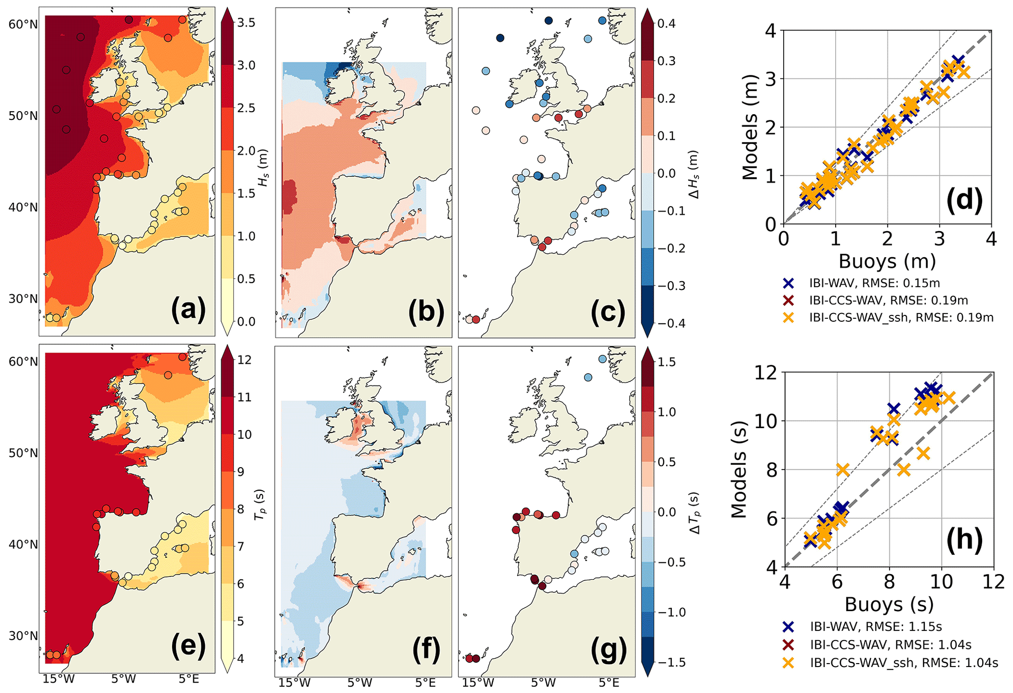
Figure 2 (a–d) The mean significant wave height (H_s, in m) over the 1993–2014 period for (a) IBI-CCS-WAV for the domain and wave buoys for the circles; (b) differences between IBI-CCS-WAV and the reanalysis; (c) bias between IBI-CCS-WAV and wave buoys at buoy locations; (d) scatter plot at each wave buoy location of IBI-CCS-WAV (red marks), IBI-CCS-WAV_ssh (yellow marks), and the reanalysis (blue marks) vs. observations. (e–h) The corresponding figures for peak period (T_P, in s); (h) must be interpreted with caution, as the observations are scarce. For (b) and (f), the domain is limited to the domain distributed by the Copernicus Marine Service, with a cut in the northern part. In (d) and (h), the thin dashed lines indicate the 20 % error margin. The RMSE is calculated as the root-mean-squared deviations from the line y=x (spatial RMSE).

Between 35 and 45^∘ N in the deep ocean, IBI-CCS-WAV nevertheless exhibits a positive bias for the mean significant wave height compared to the reanalysis (Fig. 2b). This feature is due to the westerlies taken from the global climate model (Table 1 and Appendix A) that are shifted southward. As such, the significant wave heights used as boundary forcings are slightly overestimated in the southern domain and underestimated in the northern domain around Ireland, leading to an overall relative error of 10 %. Differences in the mean state of significant wave height and peak period between IBI-CCS-WAV and the reanalysis are often larger in coastal zones and can reach a relative error of 20 % in the Gulf of Cadiz (Fig. 2b, f). These differences in coastal zones are mainly due to the different forcing in the surface currents (Table 1), which is particularly different around the Strait of Gibraltar. For the mean peak period, around the Iberian Peninsula, the biases between IBI-CCS-WAV and the reanalysis (Fig. 2f) seem to be in contradiction with those found between IBI-CCS-WAV and the wave buoys (Fig. 2g). Toledano et al. (2021) also reported large errors between the reanalysis and wave buoys over the mean wave period in northern Spain. The uncertainty appears to be large in this region, and IBI-CCS-WAV is within the uncertainty range.

The IBI-CCS-WAV_ssh simulation is compared to the buoy data in the scatter plots (Figs. 2d, h and 3d, h), but the performance of IBI-CCS-WAV_ssh is similar to that of IBI-CCS-WAV, since the buoys are mostly located in deep waters (Sect. 4).

The 99th percentile

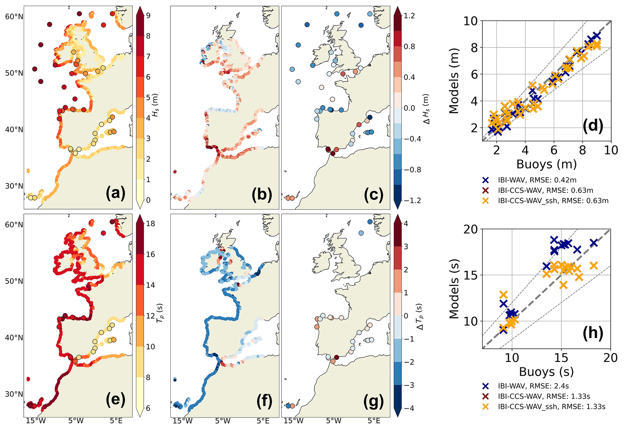
Figure 3 (a–d) The 99th percentile (based on hourly outputs) coastal significant wave height (H_s, in m) over the 1993–2014 period for (a) IBI-CCS-WAV for the domain and wave buoys for the circles; (b) differences between IBI-CCS-WAV and the reanalysis; (c) bias between IBI-CCS-WAV and wave buoys at buoys locations; (d) scatter plot at each wave buoy location of simulations IBI-CCS-WAV (red marks), IBI-CCS-WAV_ssh (yellow marks), and the reanalysis (blue marks) vs. observations. (e–h) The corresponding figures for the coastal peak period (T_P, in s); (h) must be interpreted with caution, as the observations are scarce. Note the different color bars in (a)–(c) and in (e)–(g). For (b) and (f), the domain is limited to the domain distributed by the Copernicus Marine Service, with a cut in the northern part. In (d) and (h), the thin dashed lines indicate the 20 % error margin. The RMSE is calculated as the root-mean-squared deviations from the line y=x (spatial RMSE). Note that the color scales for the biases are larger than for Fig. 2.

The extreme significant wave height and extreme peak period of IBI-CCS-WAV are validated in Fig. 3 and are satisfactorily reproduced by the model, with an overall relative error of 14 % and 9 % for H_s and T_P, respectively (Fig. 3d, h). These values are comparable to the relative errors of 13 %, 18 %, and 20 % found in Lobeto et al. (2021) for the 1-in-5-, 1-in-20-, and 1-in-50-year significant wave heights in global wave simulations. The performance of both IBI-CCS-WAV and the reanalysis is close, with a slight underestimation of the largest extreme significant wave heights. In addition, IBI-CCS-WAV seems to overestimate the smallest 99th percentile of significant wave height, particularly in the Gulf of Cadiz and around the Strait of Gibraltar, where the values are 1 m too large (Fig. 3b, c). This feature is also mainly associated with the different current forcing in this very complex zone. For the extreme peak periods, differences of 3 s (relative error of 20 %) are found along the Atlantic coasts between IBI-CCS-WAV and the reanalysis (Fig. 3f). However, this feature seems to be related to an overestimation of the extreme peak periods in the reanalysis, as the differences do not appear when IBI-CCS-WAV is compared to wave buoys (Fig. 3g, h). This overestimation is reported in Toledano et al. (2021), in which the reanalysis is validated.

3.1.2 Wave roses

Directional distributions are validated on wave roses at two locations in the Atlantic Ocean marked on Fig. 1a (Fig. 4). The focus is only on the IBI-CCS-WAV simulation, since the two buoys are located in deep waters (Fig. 1a). Since both sites located in the Atlantic Ocean are exposed to the westerlies, the wave roses indicate dominant waves in the west, west-northwest, and west-southwest directions. For the North Atlantic buoy 6200093, both the reanalysis and IBI-CCS-WAV tend to have a southward-direction bias compared to the wave buoy associated with a smaller directional spread of the biggest waves coming from the north (Fig. 4a, b and c). For the reanalysis, the dominant wave direction is west, as for the buoy (Fig. 4a and c), while in IBI-CCS-WAV the dominant wave direction is west-southwest (Fig. 4b). For the Belle-Ile buoy 6200074, the west direction represents 70 % of occurrence in IBI-CCS-WAV against 60 % for the wave buoy (Fig. 4d and e). This difference comes from waves with a significant wave height of less than 2 m found in the west-northwest direction for the buoy data.

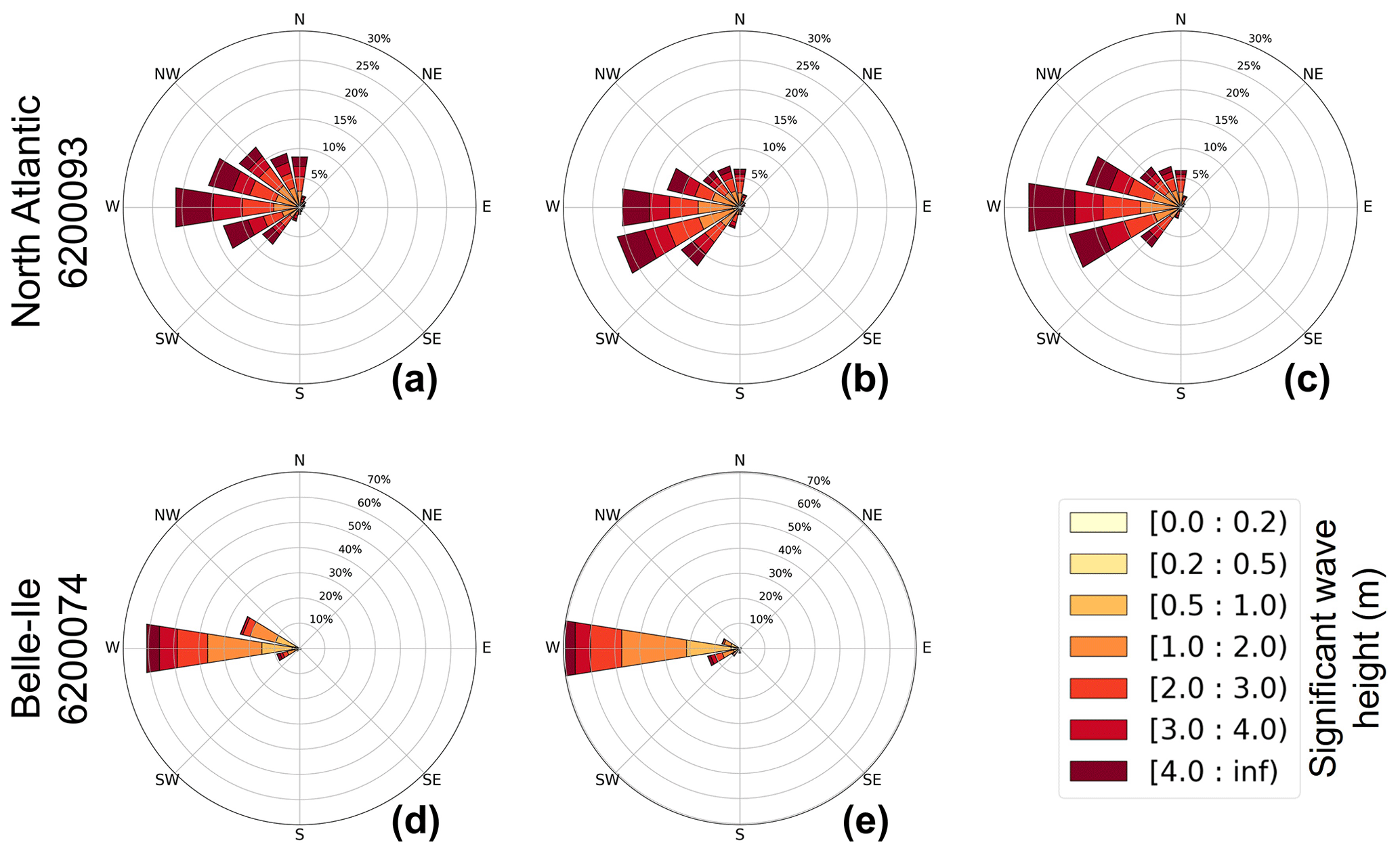
Figure 4 Directional distributions of significant wave height at star locations of Fig. 1a: North Atlantic buoy 6200093 (a–c), Belle-Ile buoy 6200074 (French Atlantic coast, (d, e)). First column represents the wave roses based on wave buoy data over the (a) 2003–2022 and (d) 2005–2022 periods. Second column (b, e) represents the roses for IBI-CCS-WAV over the 1993–2014 period, and last column (c) is for the reanalysis over the 1993–2014 period. Different periods are chosen for the wave buoys because of the lack of data for the wave direction over the 1993–2014 period. Wave roses at the North Atlantic buoy 6200093 location were computed using mean wave direction. Wave roses at the Belle-Ile buoy 6200074 location were computed using the wave direction at spectral peak, as this was the data provided by the wave buoy. However, this variable was not an output of the reanalysis. Colors indicate the wave height distribution in each direction bin.

In summary, both the IBI-CCS-WAV and IBI-CCS-WAV_ssh regional wave simulations show good performance compared to the reanalysis and wave buoys, although observations are scarce.

3.2 Regional wave projections of IBI-CCS-WAV under the SSP5–8.5 climate change scenario

Regional projections for the end of the 21st century are now presented for IBI-CCS-WAV under the SSP5–8.5 climate change scenario for the significant wave height, peak period, and mean wave direction validated in Sect. 3.1. By driving our regional simulations with a single global climate model, the aim of the study was not to provide regional wave projections with characterized uncertainties over the domain. Nonetheless, we verified that our regional projections were consistent with other large-scale studies. Projected changes for IBI-CCS-WAV_ssh are not presented in this section because they are not directly comparable to other studies that do not include sea level variations; this simulation will be used to characterize the impact of sea level changes on waves in Sect. 4.

3.2.1 Projected changes in mean and extreme significant wave height and peak period

Projected changes in mean and extreme significant wave height and peak period are illustrated in Fig. 5 for the end of the century under the SSP5–8.5 climate change scenario. Projected changes are globally consistent with other studies (Lobeto et al., 2021; Melet et al., 2020a; Morim et al., 2019; Aarnes et al., 2017; Casas-Prat et al., 2018), with a large decrease in mean significant wave height and peak period in the Atlantic Ocean and Mediterranean Sea (Fig. 5). Projected changes in the mean peak period can reach a decrease of −0.5 s or −6 % in the southern domain in comparison to the historical period (Fig. 5c). For the mean significant wave height, projected changes are largest in the northwestern domain and can reach −30 cm or −10 % (Fig. 5a). Changes in wave height and peak period result from changes in the wave spectrum composed by different wave regimes (e.g., swells and wind waves). The large decrease in significant wave height is due to a general decline in wind speed forcing from the global climate model forcing (Table 1) over the domain and in the North Atlantic Ocean, inducing changes in both wind waves and swells in the domain (not shown). The decrease in wind speed under the SSP5–8.5 scenario is consistent with other CMIP6 models projections (Carvalho et al., 2021).

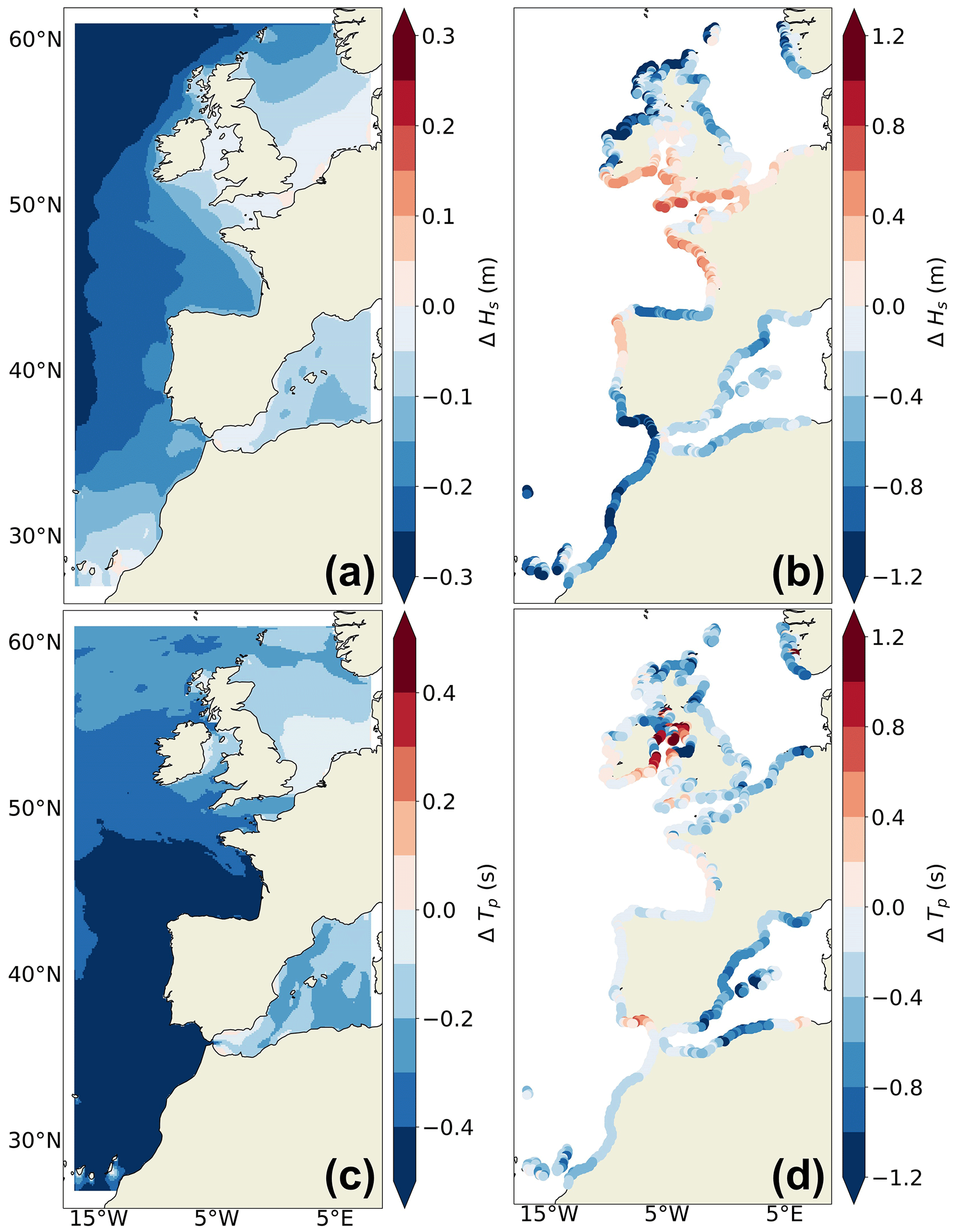
Figure 5 Projected changes in mean (a, c) and coastal extreme 1-in-100-year (b, d) wave conditions for the 2081–2100 period (relative to 1986–2005) under the SSP5–8.5 climate scenario for (a, b) the significant wave height (ΔH_s, in m) and (c, d) the peak period (ΔT_P, in s).

Projected changes in the extremes are spatially substantially different from those in the mean state, as reported in Morim et al. (2018). This is associated with different changes in the extreme wind speed forcing compared to those in the mean state (not shown). For example, a large decrease in extreme wind speed (Fig. A2b) and thus in significant wave height of more than 1 m or 12 % is located in the North Atlantic, south of 45 and north of 55^∘ N (Fig. 5b). This is consistent with other studies (Aarnes et al., 2017; Meucci et al., 2021) in which the largest decrease in extreme significant wave height is also found in the southern domain. In the English Channel, Celtic Sea, and French Atlantic coasts, the model even exhibits an increase in extreme significant wave height that has not been reported in other studies. This increase is, however, consistent with projected changes in extreme wind speed shown in Fig. A2b for the English Channel for the forcing global climate model. Projected changes in the extreme peak period are moderate, as they generally represent a decrease of less than 2.5 % (Fig. 5d).

3.2.2 Projected changes in wave roses

Projected changes in directional wave height distributions are presented on wave roses at the two locations validated in Sect. 3.1 (Fig. 6). The wave roses are decomposed into wind wave and primary swell contributions. The roses due to the primary swell contribution (Fig. 6b and d) are very close to those of Figure 4, showing that the primary swell is the main contributor to significant wave height in the Atlantic Ocean. At the end of the century, the wave rose at the Belle-Ile buoy exhibits a clockwise shift of 20^∘ in the main direction of the wind wave, changing from a west-southwest to a west-northwest direction (Fig. 6c). In this zone, a clockwise shift in the wave direction has already been documented in Morim et al. (2019). This shift seems to come mainly from small waves with a significant wave height of less than 50 cm. For the primary swell at Belle-Ile, we observe a slight strengthening of the swell from the west direction associated with a reduction of the wave components coming from the southwest (Fig. 6d). Projected changes are different for North Atlantic buoy, showing a slight strengthening of the wind wave heights in the southwest and west-southwest direction bins (Fig. 6a) and a larger strengthening (occurrence increased by 5 %) of the primary swell heights in the west direction (Fig. 6b).

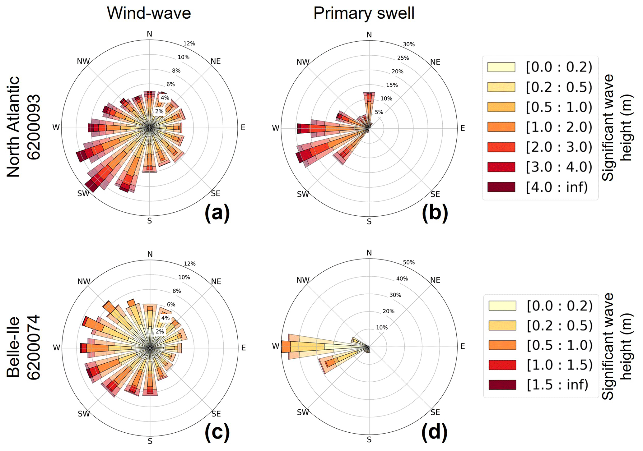
Figure 6 Projected changes (SSP5–8.5 scenario) in directional distribution of significant wave height for the 2081–2100 period (narrow-angle bins, dark colors) relative to 1986–2005 (wide-angle bins, pale colors) in IBI-CCS-WAV at star locations of Fig. 1a: North Atlantic buoy 6200093 (a, b) and Belle-Ile buoy 6200074 (c, d). The significant wave height and mean wave direction have been classified according to their origin: wind wave (a, c) and primary swell (b, d). Colors indicate wave height distribution in each direction bin.

In summary, we observe a general decrease in mean and extreme significant wave height and peak period over the domain, as well as a clockwise mean wave direction change along the French Atlantic coasts. These projected changes are coherent with previous studies.

4 Results: impact of sea level changes on waves considered in the regional wave model

We now assess the methodological question of the impact on wave characteristics of considering hourly sea level variations in the regional wave model. For that purpose, the two simulations that do and do not account for the impact of sea level changes on waves (IBI-CCS-WAV and IBI-CCS-WAV_ssh, respectively) are compared in terms of significant wave height and peak period for both the mean state and extreme events.

4.1 Impact for the entire coastal domain

4.1.1 Mean state

Except for a few locations, such as the Bay of Mont-Saint-Michel or the mouth of some rivers in the United Kingdom, there is almost no impact of including sea level variations in the wave model on the mean state of waves conditions for the historical period (Fig. 7a, c). This suggests that there is no strong non-linear effect of sea level on waves that would make a difference to the 20-year mean state for the majority of the coastal domain with our model settings.

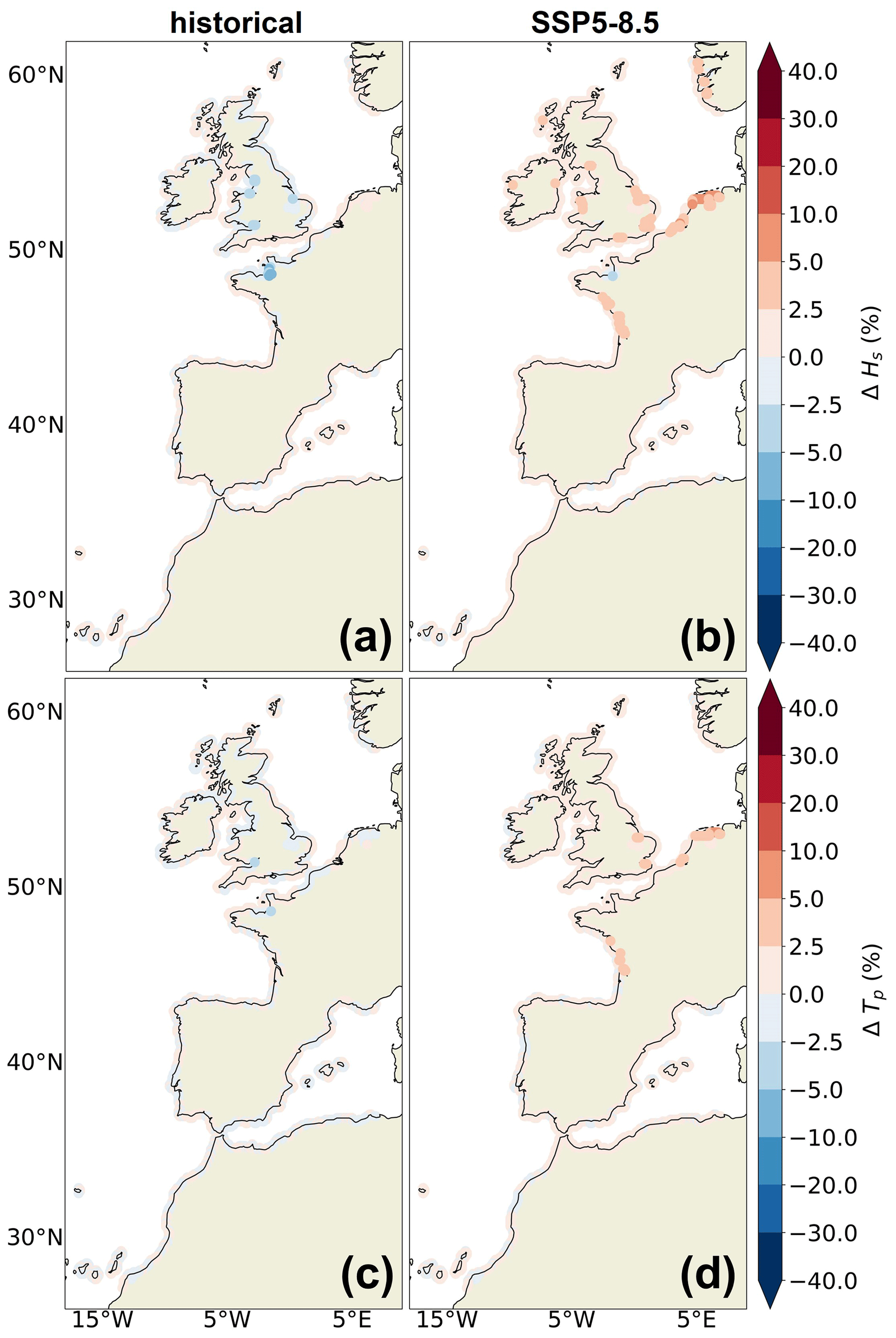
Figure 7 Mean state. Impact of the inclusion of hourly sea level variations in the wave model on the mean state of (a, b) significant wave height (ΔH_s, in %) and (c, d) peak period (ΔT_P, in %). (a, c) The relative differences of mean state between IBI-CCS-WAV_ssh and IBI-CCS-WAV for the 1986–2005 period. (b, d) The relative differences of mean state between IBI-CCS-WAV_ssh and IBI-CCS-WAV for the 2081–2100 period under the SSP5–8.5 scenario. Note that the color bars of Figs. 7 and 9 are not linear and are identical to facilitate the comparisons between the two figures.

At the end of the century, projected sea level changes in the regional ocean simulations used as forcing (Table 1, Sect. 2.3) are mainly dominated by the mean sea level rise (sterodynamic and barystatic sea level rise), with rather small changes in tides and storm surges (Chaigneau et al., 2022). This increase reaches approximately +80 cm in our region in 2100 compared to the 1986–2005 period under the SSP5–8.5 scenario. Therefore, since IBI-CCS-WAV and IBI-CCS-WAV_ssh are forced by the same winds and thus the same storms, Fig. 7 mainly shows the impact of mean sea level rise on the mean wave conditions. This long-term mean sea level rise has an overall small effect on the large continental shelf where shallow- and intermediate-water dynamics predominate (Fig. 1a). Future mean significant wave heights are up to +8 % (+4 cm) higher in IBI-CCS-WAV_ssh than in IBI-CCS-WAV along the French Atlantic coasts and in the southern North Sea (Fig. 7b). This result is consistent with Arns et al. (2017), who showed that changes in water depth induced by sea level rise resulted in greater wave amplitudes near the coast. The impact of sea level on future mean peak periods is even smaller, with differences of up to +4 % (or 0.05 s) (Fig. 7d). In the southern North Sea, projected changes in both significant wave height and peak period are small (< 10 cm, Fig. 5a). The small impact of the sea level changes on waves (+3 cm, +0.05 s) is therefore not negligible.

4.1.2 Extreme conditions: 1-in-100-year return level

Considering extreme events, the impact of sea level on significant wave heights over the historical period is substantially more important (Fig. 8a). The coastal points of the wide continental shelf are significantly impacted (southern North Sea, English Channel, seas around the United Kingdom, and French Atlantic coasts). This is particularly the case for macro-tidal locations (Fig. 1b) such as the Bay of Mont-Saint-Michel, the Bristol Channel, and the eastern Irish Sea. In these areas, the historical 1-in-100-year event of significant wave height is up to +30 % (+40 cm) higher when considering sea level variations, mostly dominated by tidal variations, as discussed in Sect. 4.2. At the end of the century, the impact of including hourly sea level variations on the future 1-in-100-year level wave events is even larger, mostly due to the combined effect of the tides and mean sea level rise. Future extreme significant wave heights are increased by up to +40 % or +60 cm (Fig. 8b). On the contrary, extreme peak periods are negligibly impacted by the non-linear effect of sea level with waves (Fig. 8c, d).

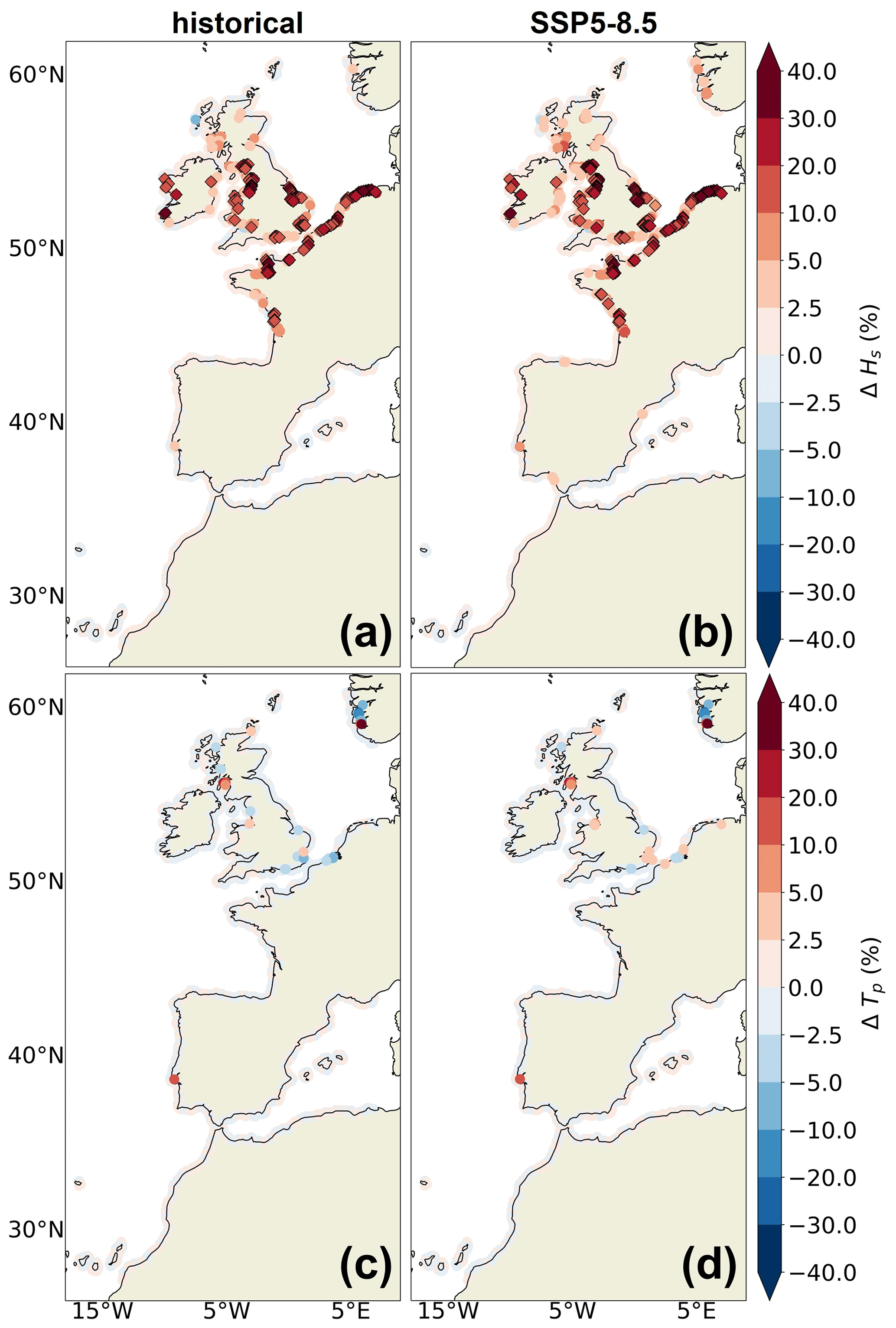
Figure 8 Extreme conditions. Impact of the inclusion of hourly sea level variations in the wave model on the 1-in-100-year return level of (a, b) significant wave height (ΔH_s, in %) and (c, d) peak period (, ΔT_P, in %). (a, c) The relative differences of the 1-in-100-year return level between IBI-CCS-WAV_ssh and IBI-CCS-WAV for the 1986–2005 period. (b, d) The relative differences of the 1-in-100-year return level between IBI-CCS-WAV_ssh and IBI-CCS-WAV for the 2081–2100 period under the SSP5–8.5 scenario. The large diamonds represent the locations where the differences between both simulations are significant (i.e., where the confidence intervals associated with the 100-year return level calculation are disjointed). Note that the color bars of Figs. 7 and 9 are not linear and are identical to facilitate the comparisons between the two figures.

4.2 Example of the impact on extreme events at two specific locations

The largest impact of including sea level variations in the wave model is found during extreme events, as shown in Fig. 8. We now focus on two specific French regions where an impact has been identified in Fig. 8. In the Bay of Mont-Saint-Michel, strong hourly sea level variations occur due to the large tidal range in the region (10 m, Fig. 1b). For the French Atlantic coast, the tidal range is large (4 m, Fig. 1b) but smaller than in the Bay of Mont-Saint-Michel.

Time series of significant wave height and peak period during an extreme-significant-wave-height event are shown in Fig. 9. Note that, as the global climate model forcing is not in phase with observation in terms of internal climate variability, the event selected cannot be compared directly to observations. Nevertheless, we have validated in Sect. 3.1 that the amplitude of simulated extreme events was realistic. The significant wave height time series from IBI-CCS-WAV_ssh oscillate hourly, in phase with the tide, illustrating the consideration of hourly sea levels in the regional wave model (Fig. 9a, b). In the case of the Bay of Mont-Saint-Michel, the largest significant wave height reached on the day of 25 October 1993 at high tide is 1 m higher (+30 %) in IBI-CCS-WAV_ssh than in IBI-CCS-WAV due to the large tidal range (Fig. 9a). As the Bay of Mont Saint-Michel has one of the highest tidal ranges in the IBI domain, the observed impact of sea level variations on waves corresponds to the upper limit with the parameters of our model. For the French Atlantic coast, in this specific case, the extreme event of significant wave height occurs at low tide during a medium neap tide, so the impact of hourly sea level variations on the extreme significant wave height is null. In both cases, it can be pointed out that the increase in wave height occurs at high tide. These results are in agreement with Lewis et al. (2019) and Calvino et al. (2022), who both showed a significant increase in wave height at high tide at a finer scale. In Calvino et al. (2022), this impact seems to be explained mainly by the effect of bottom friction, which is less important at high tide, as the water column is higher. In the case of Arns et al. (2017), waves are higher when sea level increases (e.g., at high tide) because they break closer to the shore. In our case, additional analyses would be needed to understand which process included in the model (Sect. 2.1) is the most responsible for the non-linear effect of sea level with significant wave height. In both IBI-CCS-WAV and IBI-CCS-WAV_ssh, diurnal variations of the peak period appear due to tidal current that shortens or lengthens the dominant wave period (Ardhuin et al., 2012), but the impact of sea level variations is almost null (Fig. 9c, d).

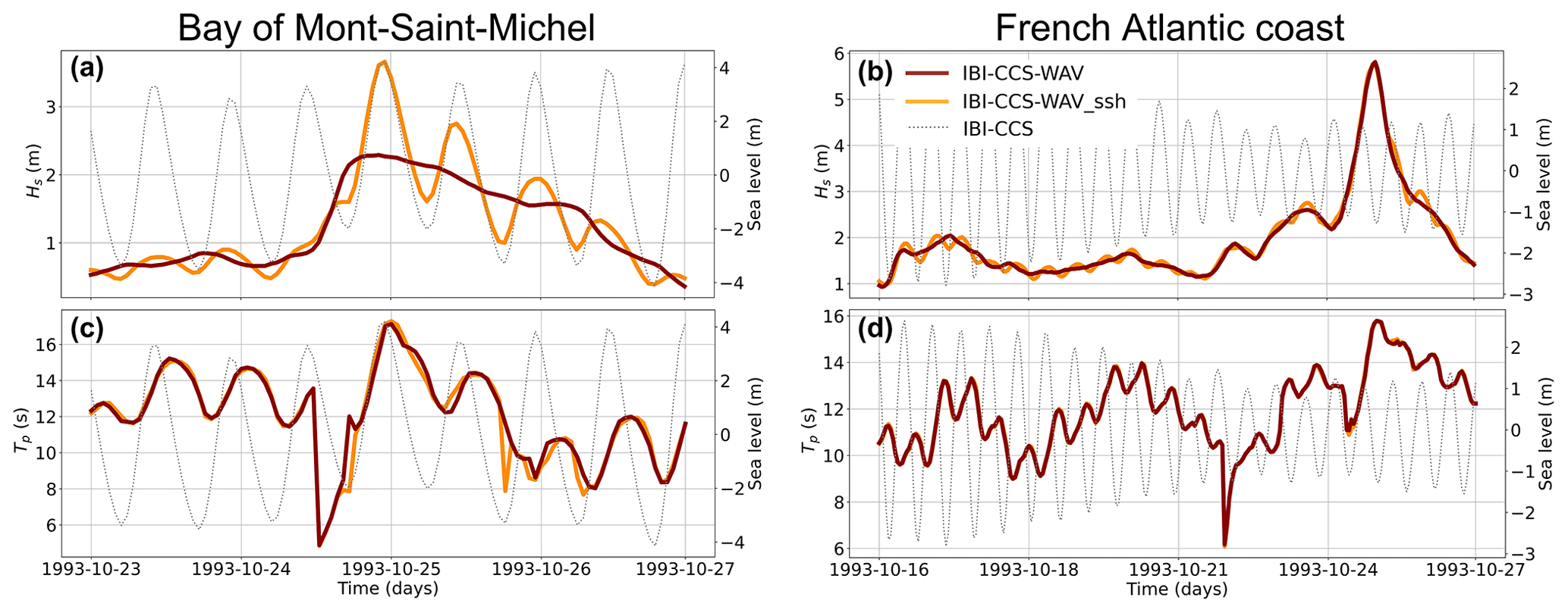
Figure 9 Time series of incoming wave conditions for the Bay of Mont-Saint-Michel (a, c) and for the French Atlantic coast (b, d) during an extreme-significant-wave-height event of October 1993. The two locations are marked on Fig. 1b. The curves represent IBI-CCS-WAV (dark-red curve) and IBI-CCS-WAV_ssh (dark-yellow curve) for (a, b) the significant wave height (H_s, in m) and (c, d) the peak period (T_P, in s). Sea level variations are shown in thin dotted gray lines on the right y axis for each panel.

To better assess the impact of sea level variations on the extreme significant wave heights, return period curves are displayed in Fig. 10 for the two locations. The higher the return periods, the larger the impact of sea level changes on waves. For instance, in the Bay of Mont-Saint-Michel, the 1-in-100-year return level of significant wave height is +60 % larger when considering sea level variations in the wave model (Fig. 10a). At the end of the century, the differences between the two simulations are even larger and can reach +70 %, mainly due to the mean sea level rise of about +80 cm under the SSP5–8.5 scenario. The curves also indicate that considering the interaction of sea level on waves modifies the shape of the return period curve, which may have important implications for the future amplifications of extreme events.

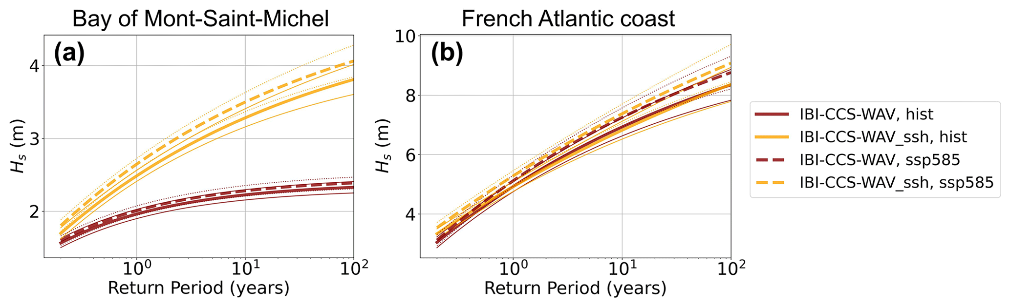
Figure 10 Return period curves of significant wave height (H_s, in m) for IBI-CCS-WAV (dark-red curves) and IBI-CCS-WAV_ssh (dark-yellow curves) for (a) the Bay of Mont-Saint-Michel and (b) the French Atlantic coast (Fig. 1b). The solid lines represent the 1985–2006 period, and the dashed lines represent the 2081–2100 period under the SSP5–8.5 scenario. The thin solid and dashed lines are the confidence intervals (corresponding to 1 sigma confidence) associated with the extreme-value analysis (EVA). The differences between IBI-CCS-WAV and IBI-CCS-WAV_ssh are considered to be significant when the confidence intervals associated with the return level calculation are disjointed.

5 Discussion

5.1 Model limitations

The use of a single-forcing climate model does not allow us to quantify the uncertainties of the projected changes. Here, the focus of the study is not on providing a likely range of wave projected changes over the IBI domain, but rather, the focus is process-oriented. In our study, the estimation of the impact of including hourly sea level variations in the wave model is limited by several resolution aspects. The first limitation is the horizontal resolution of the wave model. The model resolution of $\mathrm{1}/\mathrm{10}$^∘ (∼ 10 km) is conditioned by the computational cost due to the length of the simulations needed to address the question of extremes on climate scales. It does not allow a very fine representation of the coastline and of the bathymetry in the coastal zones. Moreover, the regional ocean model (Table 1 and Appendix A) used for the surface currents and sea level forcing does not allow for dry areas. Therefore, a minimal bathymetry is set to 6 m to run the ocean model with tides (Chaigneau et al., 2022). We chose to apply the same minimal bathymetry of 6 m in the regional wave model to maintain consistency between both regional ocean and wave models. In fact, because it would have been unrealistic to have a bathymetry of 1 m within a 10 km grid point, the minimum bathymetry (6 m) also allows us to maintain a realistic balance between the 10 km horizontal resolution and the water depth. This results in fewer areas of shallow and intermediate water in the wave model and thus less of an effect of sea level variations on the waves. The implementation of wetting and drying (O'Dea et al., 2020), allowing for dry areas in NEMO version 4.2, should improve this limitation on the ocean model and therefore on the wave model. Another limitation is the resolution of the atmospheric forcing from the global climate model (Table 1). Given that winds are the major drivers of extreme-wave events in our study, even with a relatively high-resolution climate model forcing, the resolution of 50 km for the atmospheric drivers implies that generated waves are more representative of a large-scale forcing than of coastal processes.

For all these reasons, the estimates provided in this study only partially represent the processes responsible for the non-linear interaction of sea level with waves, and the results found in this study are not representative of any purely local situation at the coast but rather provide regional information. A second step of dynamical downscaling at higher resolution would be necessary to overcome such resolution limitations.

5.2 Impact of waves on sea level

The aim of the study was to better understand the non-linear interactions between waves and sea level. In the modeling framework of the paper, only the effect of sea level on waves is accounted for. However, both are coupled in reality, with waves impacting on sea level. For instance, Bonaduce et al. (2020) have studied the contribution of wave processes to sea level variability over the European Seas with ocean–wave coupled simulations at an eddy-resolving spatial resolution of 3.5 km. They highlighted the occurrence of mesoscale features of the ocean circulation and a modulation of the surge at the shelf break due to the effect of the wave forcing on sea level. More importantly, they also reported a large contribution of wave-induced processes to sea level extremes, which are up to 20 % higher on the European continental shelf due to these wave processes. By taking these processes into account in the ocean model, as the sea level would be higher, the impact on the wave model would be larger, meaning an increase in waves–sea-level feedbacks.

5.3 Implications of the results for coastal flooding

The results obtained in this study have shown a large impact of sea level variations on extreme significant wave heights. Wind waves and swell contribute to extreme sea levels at the coast via wave setup and run-up (Dodet et al., 2019), combined with tides, storm surges, and mean sea level changes. Marine-flooding hazards cannot be quantified based on wave contributions alone, but these contributions can locally partially enhance sea level changes at the coast (Melet et al., 2020a). Our results show that extreme significant wave heights are strongly influenced by the effect of sea level on waves in coastal areas subject to large sea level variations or on wide continental shelves. Depending on the region (wave regimes, sign of the extreme-wave projected changes, local ocean processes involved, and amplitude of projected changes in local sea level), the impact of the sea level changes on waves could be important to consider for present and future flooding hazards (e.g., for threshold exceedance calculations). For instance, future wave conditions and therefore coastal flooding could be affected in areas where large changes in tides are projected, such as in the China Sea and the Gulf of Saint Lawrence (Pickering et al., 2017; Haigh et al., 2020). Future extreme waves could also be significantly impacted in areas subject to large relative mean sea level rise, such as along the eastern coasts of the United States, the Gulf of Mexico, and the Caribbean Sea, where a rise of +1.4 m is expected by the end of the century under the SSP5–8.5 scenario (Fox-Kemper et al., 2021).

6 Conclusions

Several studies have shown that water depth changes can induce changes in the wave field at a fine spatial scale (Hoeke et al., 2015; Arns et al., 2017; Lewis et al., 2019; Idier et al., 2019; Calvino et al., 2022). The aim of this paper was to characterize, at a larger scale, the sensitivity of historical and projected sea states to the sea level changes (tides, storm surges, and mean sea level changes) notably during extreme events. To address this question, a regional wave model has been adapted to include sea level variations over the northeastern Atlantic for the 1970–2100 period. This is one of the first studies assessing the impact of sea level changes on wave conditions at such a regional large scale.

First, the regional wave model is presented and validated over the 1993–2014 period. Comparisons to observations and a wave reanalysis show overall good performance of the model. Secondly, as we used a single-forcing climate model, projected regional changes in mean and extreme-wave conditions are compared to previous studies. They are shown to be representative of other published projections over the northeastern Atlantic region, with a general decrease in mean and extreme significant wave height and peak period under the SSP5–8.5 scenario.

The impact of including hourly sea level variations in the wave model is assessed over the historical period and for 21st century projections for the mean state and extremes of wind wave characteristics. The impact on the mean state is found to be weak in general over the historical period and at the end of the 21st century. Over the northeastern Atlantic, mean sea level rise and, to a lesser extent, changes in tidal amplitudes and storm surges reach approximately +80 cm in 2100 compared to the 1986–2005 period for the SSP5–8.5 scenario. This increase leads to mean significant wave heights up to +3 cm (or +6 %) higher along the French Atlantic coasts and in the southern North Sea by the end of the 21st century. The impact of sea level variations is substantially more important for extreme significant wave heights over the wide continental shelf, where shallow-water dynamics prevail, and particularly in large-tidal-range areas. For example, in the Bay of Mont-Saint-Michel, where the tidal range is 10 m on average, extreme significant wave heights are found to be larger by 1 m (or +30 %) during a historical extreme wave. Accounting for the combination of tides, storm surges, and sea level rise in the wave model also leads to higher values of 1-in-100-year significant wave heights, up to +40 % at the end of the 21st century located in the Bay of Biscay, the North Sea, around United Kingdom, and Ireland. Moreover, as the regional wave model does not have a very fine representation of the bathymetry and of the coastline and does not include the feedback of waves on sea level, the estimates provided in this study only partially represent the processes responsible for the sea-level–wave non-linear interactions. Overall, the inclusion of water level variations in the wave model had almost no impact on the peak period.

In conclusion, our results advocate for the inclusion of sea-level–wave non-linear interactions in modeling studies of wave extremes at this resolution or higher, in particular when extreme significant wave heights are of interest. These non-linear interactions should be accounted for when threshold exceedances are calculated, for example in order to prevent coastal flooding or to build coastal protection structures in a climate change context.

Appendix A: External forcings used to produce the regional wave simulations

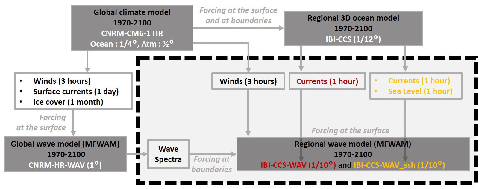
Figure A1 Sketch of the downscaling strategy explaining the links between the different simulations used in this study.

A1 Wave forcing from CNRM-HR-WAV global wave simulations

The regional wave simulations IBI-CCS-WAV and IBI-CCS-WAV_ssh described in Sect. 2.2 and 2.3 are forced at lateral boundaries by 3-hourly wave spectra information from CNRM-HR-WAV global wave simulations (Fig. A1, Table 1). CNRM-HR-WAV simulations are produced over the 1970–2100 period using the MFWAM wave model (Sect. 2.1) at a 1^∘ resolution. These simulations are forced by 3-hourly surface winds ($\mathrm{1}/\mathrm{2}$^∘), monthly sea ice cover ($\mathrm{1}/\mathrm{4}$^∘), and daily ocean surface currents ($\mathrm{1}/\mathrm{4}$^∘) taken from the CMIP6 CNRM-CM6-1-HR global climate simulations (Voldoire et al., 2019; Saint-Martin et al., 2021). The historical simulation of CNRM-CM6-1-HR is used over the 1970–2014 period. Then, over the 2015–2100 period, the SSP5–8.5 climate change scenario simulations are used (O'Neill et al., 2016).

CNRM-HR-WAV simulations use 2 min gridded global topography data from ETOPO2/NOAA (NOAA National Geophysical Data Center, 2006). The model grid has a constant spacing in longitude but is compressed in latitude to maintain a constant resolution (Bidlot, 2012). A wave growth calibration was performed to adjust the mean significant wave height of CNRM-HR-WAV to the Copernicus Marine Service WAVERYS wave reanalysis (Law-Chune et al., 2021) over the IBI domain. The wave spectrum is discretized in 24 directions and 30 frequencies, starting from 0.035 up to 0.58 Hz. Classical integrated wave parameters such as significant wave height (H_S) or peak period (T_p) are output at every 3 h from CNRM-HR-WAV.

A2 Atmospheric forcing from CNRM-CM6-1-HR global climate model

Regional wave projections are driven by the same 3-hourly surface winds as CNRM-HR-WAV (Sect. A1.1), produced by the CNRM-CM6-1-HR global climate model (Voldoire et al., 2019; Saint-Martin et al., 2021), which is part of the CMIP6 database. The use of a global climate model with a higher spatial resolution compared to the typical coarse resolutions of CMIP5 and 6 models was interesting for the atmosphere ($\mathrm{1}/\mathrm{2}$^∘) and notably for the intensity of the winds.

By driving our simulations with only one global climate model simulation, the aim of the study was not to characterize the uncertainties of wave projected changes over the IBI domain but rather to discuss the impact of the sea level changes on the downscaled projections. However, before using the winds to force the global and regional wave models, we verified that CNRM-CM6-1-HR was consistent with other CMIP6 global climate models, particularly in terms of extreme winds and their projections. A comparison of extreme winds (99th percentile) between CNRM-CM6-1-HR, some other CMIP6 global climate models, the atmospheric reanalysis ERA5 (Hersbach et al., 2020), and wind observations from wave buoys (Wehde et al., 2021) is performed at different locations in the IBI region (Fig. A2a). The three different locations considered (shown in Fig. 1) are chosen along storm trajectories in the northeastern Atlantic and North Sea (Lozano et al., 2004). Figure A2a shows that CNRM-CM6-1-HR is representative of an ensemble of 21 CMIP6 models over the historical period. In general, CNRM-CM6-1-HR also agrees with ERA5, which is the reference here. However, wave buoy observations seem to be significantly different from both the global climate models and ERA5, except in the North Sea. Figure A2b shows the projected changes for the extreme wind speed at the three locations. Projected changes in extreme wind speed are quite small in all models and rather uncertain (large interquartile range). Projected changes are of the same sign for 7, 9, and 10 models out of 12 for the three boxes, respectively. In the English Channel and North Sea, CNRM-CM6-1-HR shows an increase in extreme wind speed, which is representative of the other CMIP6 models. In the North Atlantic, CNRM-CM6-1-HR exhibits a large decrease in extreme wind speed, which is in the high range (in absolute value) of CMIP6 models but still of the same sign as most models.

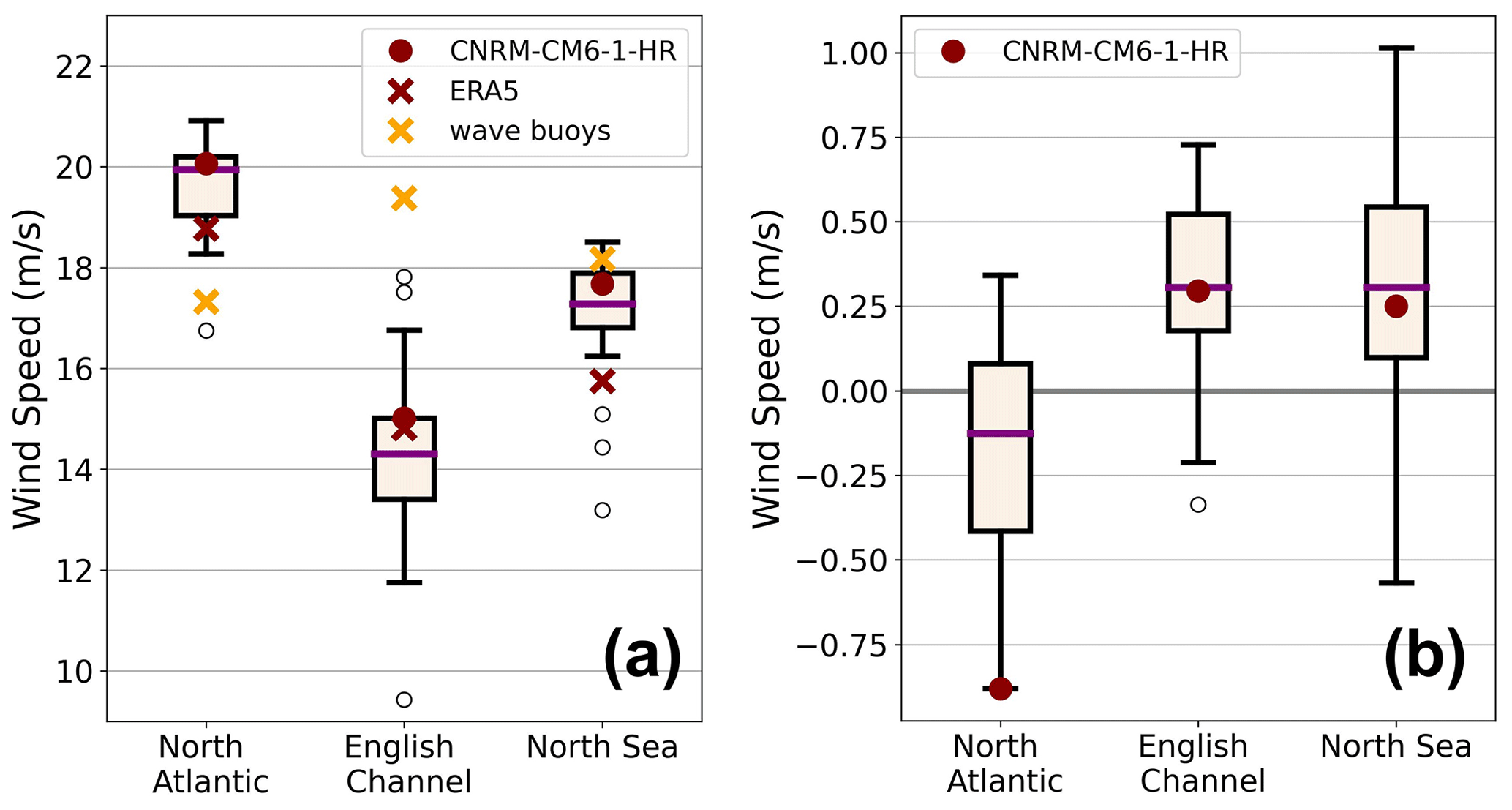
Figure A2 (a) Extreme winds (99th percentile) for CNRM-CM6-1-HR (dark-red dot), 21 different CMIP6 global climate models (black box), the atmospheric reanalysis ERA5 (dark-red cross), and wind observations from wave buoys (yellow cross) at the three locations in the IBI region marked on Fig. 1a for the 1993–2014 period. The 2011–2022 period was chosen for the wave buoy in the North Sea, as it was the only period available. (b) Projected changes in extreme wind speed for CNRM-CM6-1-HR and 12 different CMIP6 climate models at the three locations marked on Fig. 1a under the SSP5–8.5 scenario (2081–2100 vs. 1986–2005). The selected CMIP6 climate models are those with 3-hourly atmospheric outputs. In (a) and (b), the purple line represents the median, the black box represents the interquartile range, and the whiskers represent the last model under or above 1.5 times the interquartile range. The black circles represent the outlier models, i.e., models outside 1.5 times the interquartile range. Units are in meters per second.

A3 Ocean forcing from IBI-CCS regional ocean model

IBI-CCS-WAV regional wave projections are also forced by hourly surface current (and hourly sea level variations in the dedicated simulation IBI-CCS-WAV_ssh) of IBI-CCS, a 3D regional ocean model at a $\mathrm{1}/\mathrm{12}$^∘ horizontal resolution, itself forced by the CNRM-CM6-1-HR global climate model. IBI-CCS was implemented in Chaigneau et al. (2022) to refine sea level projections of CNRM-CM6-1-HR over the northeastern Atlantic region through a dynamical downscaling. For a more complete representation of processes driving coastal sea level changes, tides and atmospheric surface pressure forcing are explicitly resolved in IBI-CCS in addition to the mean sea level (including ocean general circulation and dynamic sea level).

Appendix B: Technical details on the implementation of sea level in the wave model

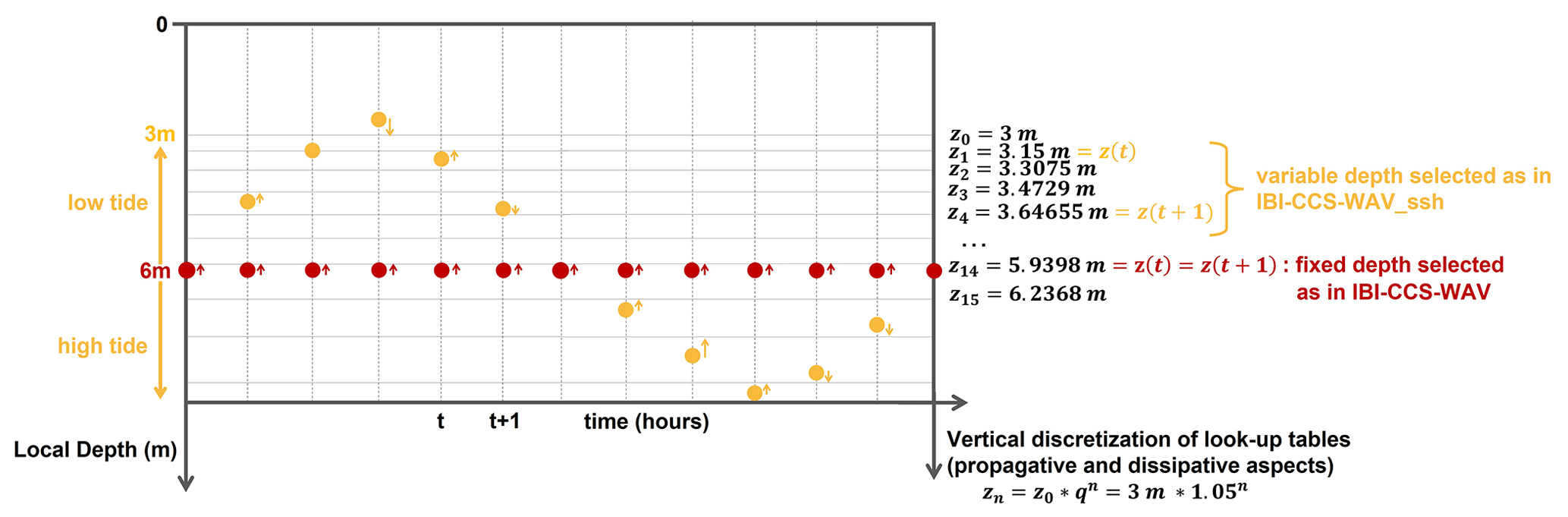
Figure B1 Schematic of the inclusion of sea level variations in the wave model for a given coastal point as a function of time. The dots represent the local depths. In red, the local depth is fixed (IBI-CCS-WAV), and in this example, the local depth is the minimum allowed, corresponding to z₆ in this example. In yellow is an example of the time evolution of the local depth corresponding to the hourly sea level variations (IBI-CCS-WAV_ssh) at the same model grid point, here dominated by a tidal signal. The thin horizontal gray lines (z₀, z₁, ..., z_n) represent the vertical discretization of the depths used in the look-up tables to obtain parameters needed for wave propagation and source terms.

The wave model operates with a look-up table system as follows: in a pre-processing step, wave propagation parameters such as group velocities and wave numbers, as well as other parameters that affect the source terms described in Sect. 2.1, are tabulated once and for all according to a list of depths (z₀, z₁, ..., z_n in Fig. B1) and frequencies. The depths that are indexed in the look-up tables are discretized following a geometric series with a first level at 3 m depth (minimum local depth allowed in the simulation with the inclusion of sea level variations) and a vertical resolution of about 15 cm in the first levels (Fig. B1) and more than 100 m in the deep ocean. They are represented by thin horizontal gray lines in Fig. B1. During the simulation, the required parameters are retrieved for each grid point from these look-up tables by selecting the closest discretized depths (thin horizontal gray lines) to the local depths (red dots in Fig. B1) estimated from the bathymetry. In intermediate to shallow waters, the inclusion of sea level affects the local depth and, consequently, the discretized depth selected in the look-up tables, which then affects the parameters required for wave propagation and source terms (Sect. 2.1).