the Creative Commons Attribution 4.0 License.
the Creative Commons Attribution 4.0 License.
 | 13 Jul 2023
Mode-1 N2 internal tides observed by satellite altimetry
Satellite altimetry provides a unique technique for observing the sea surface height (SSH) signature of internal tides from space. Previous studies have constructed empirical internal tide models for the four largest constituents M2, S2, K1, and O1 by satellite altimetry. Yet no empirical models have been constructed for minor tidal constituents. In this study, we observe mode-1 N2 internal tides (the fifth largest constituent) using about 100 satellite years of SSH data from 1993 to 2019. We employ a recently developed mapping procedure that includes two rounds of plane wave analysis and a two-dimensional bandpass filter in between. The results show that mode-1 N2 internal tides have millimeter-scale SSH amplitudes. Model errors are estimated from background internal tides that are mapped using the same altimetry data but with a tidal period of 12.6074 h (N2 minus 3 min). The global mean error variance is about 25 % that of N2, suggesting that the mode-1 N2 internal tides can overcome model errors in some regions. We find that the N2 and M2 internal tides have similar spatial patterns and that the N2 amplitudes are about 20 % of the M2 amplitudes. Both features are determined by the N2 and M2 barotropic tides. The mode-1 N2 internal tides are observed to propagate hundreds to thousands of kilometers in the open ocean. The globally integrated N2 and M2 internal tide energies are 1.8 and 30.9 PJ, respectively. Their ratio of 5.8 % is larger than the theoretical value of 4 % because the N2 internal tides contain relatively larger model errors. Our mode-1 N2 internal tide model is evaluated using independent satellite altimetry data in 2020 and 2021. The results suggest that the model can make internal tide correction in regions where the model variance is greater than twice the error variance. This work demonstrates that minor internal tidal constituents can be observed using multiyear multi-satellite altimetry data and dedicated mapping techniques.
- Article
(15176 KB) - Full-text XML
- BibTeX
- EndNote


The Moon's elliptical orbit around the Earth has an eccentricity of ≈ 0.055, with its perigean and apogean distances being about 3.63 × 10⁵ and 4.06 × 10⁵ km, respectively. The Moon completes one revolution every 27.5546 d (1 anomalistic month). The tidal constituents L2 and N2 are induced by the Moon's elliptical orbit (Doodson, 1921). They are named the smaller and larger lunar elliptical semidiurnal constituents. The L2 and N2 periods are 12.1916 and 12.6583 h, respectively (Doodson, 1921; Pawlowicz et al., 2002). M2 (12.4206 h) is based on the mean distance between the Earth and the Moon (3.84 × 10⁵ km). The L2 and N2 superposition gives the 27.5546 d perturbation because the Moon–Earth distance changes along the elliptic orbit. On a global average, the amplitudes of M2, N2, and L2 have a respective ratio of . N2 is the fifth largest tidal constituent; therefore, its impact on the ocean environment is significant. For example, in waters around New Zealand, the N2 barotropic tide has larger amplitudes than S2 (Byun and Hart, 2020, Fig. 4 therein). The superposition of N2, M2, L2, and S2 can cause perigean spring tides (king tides) and apogean neap tides, which significantly affect harbors, coastal regions, and estuaries (Wood, 1978). Including N2 internal tides can simulate the temporal variation in internal tide energetics with the Moon's elliptical motion. Theoretically, N2 may modulate M2 internal tides by ± 20 % in amplitude and by ± 40 % in energy (i.e., (1 ± 0.2)2). On average, N2 will enhance the M2-induced ocean mixing by 4 % (i.e., 0.22).
Internal tides are widespread in the ocean and affect numerous ocean processes such as diapycnal mixing, tracer transport, and acoustic transmission (Wunsch, 1975; Dushaw et al., 1995; Whalen et al., 2020). Internal tides may provide about half of the power for diapycnal mixing in the ocean interior (Munk and Wunsch, 1998; Egbert and Ray, 2000; MacKinnon et al., 2017; Kelly et al., 2021). The magnitude and geography of diapycnal mixing may modulate the large-scale ocean circulation and global climate change; therefore, it is important to study their generation, propagation, and dissipation in the global ocean (Jayne and St Laurent, 2001; Melet et al., 2016; Pollmann et al., 2019; Vic et al., 2019; de Lavergne et al., 2020; Arbic, 2022). Internal tides are annoying noise in the study of mesoscale and sub-mesoscale dynamics. In particular, it will be necessary to make internal tide correction to the Surface Water and Ocean Topography (SWOT) data, so that one can better study the sub-mesoscale dynamic processes (Fu and Ubelmann, 2014; Qiu et al., 2018; Wang et al., 2018; Morrow et al., 2019). Empirical internal tide models can be constructed using past satellite altimetry sea surface height (SSH) measurements. However, previous satellite observations focus mainly on the four largest tidal constituents: M2, S2, K1, and O1 (Dushaw, 2015; Ray and Zaron, 2016; Zhao et al., 2016; Zaron, 2019; Ubelmann et al., 2022). Dushaw (2015) attempts to map N2 internal tides using the TOPEX/Poseidon data from 1992 to 2008 but fails to obtain an empirical model because the resulting N2 internal tides are too noisy (see his Figs. 38 and 52). That work is mainly limited by the short data set available then. In this study, we will construct a reliable empirical N2 internal tide model using a larger data set and a recently developed mapping method.
The challenge of observing N2 internal tides by satellite altimetry lies in their small SSH displacements (Dushaw, 2015). Given that M2 internal tides have SSH amplitudes of 1–2 cm, N2 internal tides have only sub-centimeter SSH amplitudes. In this paper, the observation of N2 internal tides is made possible by two improvements. First, a larger SSH data set is available, thanks to almost 3 decades of multiple satellite observations since 1993. The merged data set from 1993 to 2019 is about 100 satellite years long; therefore, non-tidal errors can be significantly suppressed. Second, a recently developed mapping procedure is employed. This mapping technique extracts N2 internal tides utilizing their known frequency and theoretical wavelengths. Non-tidal errors can be significantly suppressed by both temporal and spatial filters. The resulting N2 internal tides reveal their basic features in the global ocean, although they are still noisy (compared to the much larger M2 internal tides). It is challenging (though possible) to extract L2 internal tides in some regions, which are estimated to have 1 mm SSH signals at most (5 % of M2).
The rest of this paper is arranged as follows. Section 2 describes the data and methods used in this paper. Section 3 presents and discusses the new N2 internal tides, mainly by comparing them with the well-studied M2 internal tides. Section 4 is a summary.
2.1 Data
The satellite altimetry SSH data used in this paper are collected by multiple altimetry missions from 1993 to 2021. In the order of launch time, they are TOPEX/Poseidon, ERS-1, ERS-2, Geosat Follow-On, Jason-1, Envisat, Jason-2, CryoSat-2, SARAL/AltiKa, Haiyang-2A, Jason-3, Sentinel-3A, Sentinel-3B, Haiyang-2B, and Jason-CS/Sentinel-6 (Fig. 1). The combined data set from 1993 to 2019 is about 100 satellite years long. We use the satellite along-track SSH data downloaded from the Copernicus Marine Service (https://doi.org/10.48670/moi-00146). The SSH measurements have been processed by standard corrections for atmospheric effects, surface wave bias, and geophysical effects (Pujol et al., 2016; Taburet et al., 2019). The ocean barotropic tide, polar tide, solid Earth tide, and loading tide are corrected using theoretical or empirical models (Pujol et al., 2016). Mesoscale correction (Ray and Byrne, 2010; Zhao, 2022a) is made using the gridded SSH fields downloaded from the Copernicus Marine Service (https://doi.org/10.48670/moi-00148). The satellite along-track SSH data in 2020 and 2021 are used to evaluate the new N2 internal tide model as independent data (Sect. 2.6). Extracted from the 27-year-long data, our N2 internal tide model contains only the 27-year coherent component. Their temporal variation (or incoherent component) is not addressed in this paper.
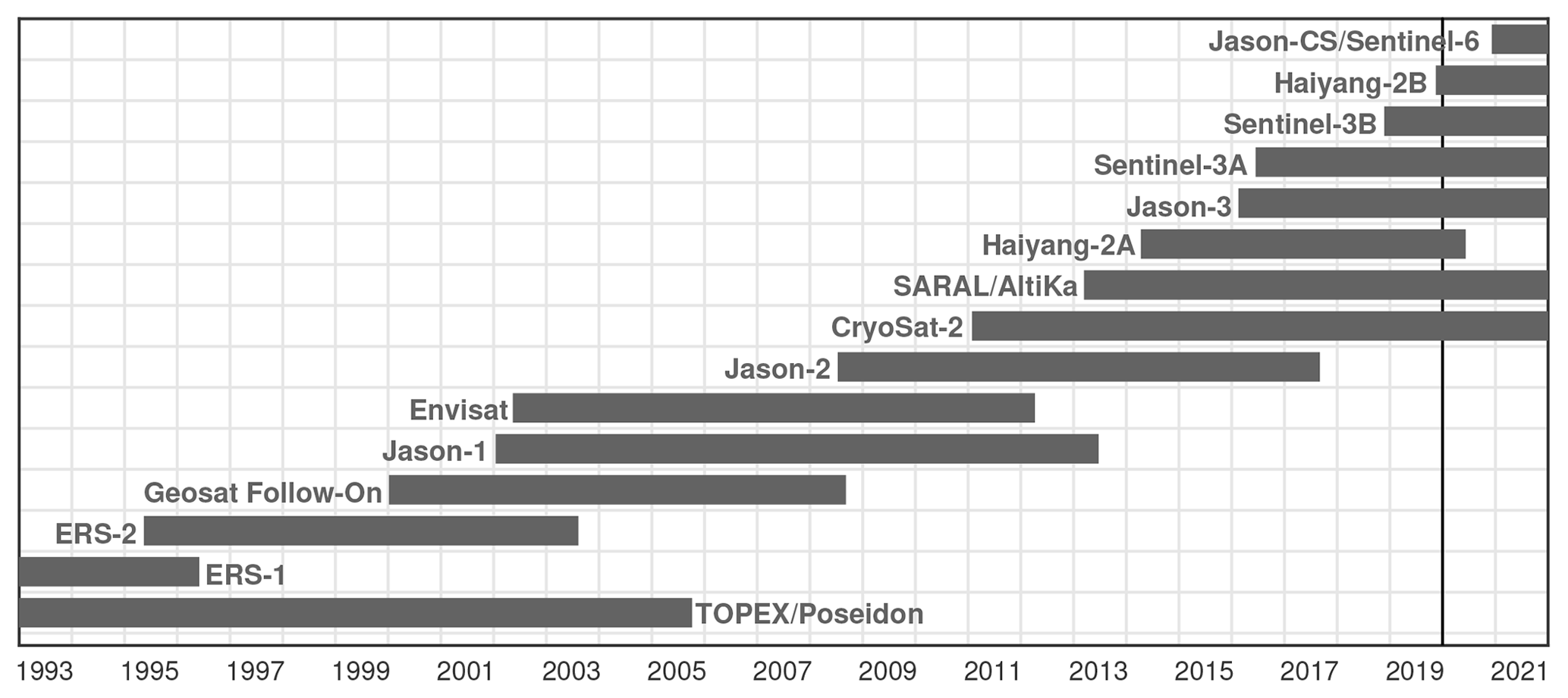
Figure 1Satellite altimetry data used in this study. The merged multiyear multi-satellite data from 1993 to 2019 are about 100 satellite years long. The altimetry data in 2020 and 2021 are taken as independent data for model evaluation.
The observation of internal tides by satellite altimetry may be affected by an issue called tidal aliasing because the satellite repeat cycles are much longer than the semidiurnal and diurnal tidal periods. Here we examine possible tidal aliasing issues with N2 and M2 internal tides. In one 160 km by 160 km fitting window (Sect. 2.2), there are typically about 7.84 × 10⁴ SSH data from multiyear multi-satellite measurements. Using their observation times, we can calculate their phase lags with respect to the N2 tidal cycle (12.6583 h). Figure 2a gives the histogram of their phase lags over one N2 tidal cycle. For comparison, Fig. 2b shows the histogram with respect to the M2 tidal cycle (12.4206 h). The results show that the SSH data overall evenly distribute over one N2 or M2 tidal cycle, without extreme biases. In particular, their distribution on M2 is smooth, suggesting that there is no tidal aliasing issues for M2. Their distribution over N2 is a little bumpy, suggesting that the resulting N2 internal tides may have larger errors. The uneven distribution stems from the orbital configurations of the satellite missions. Fortunately, as shown in this study, the new mode-1 N2 internal tides can overcome background noise in some regions.
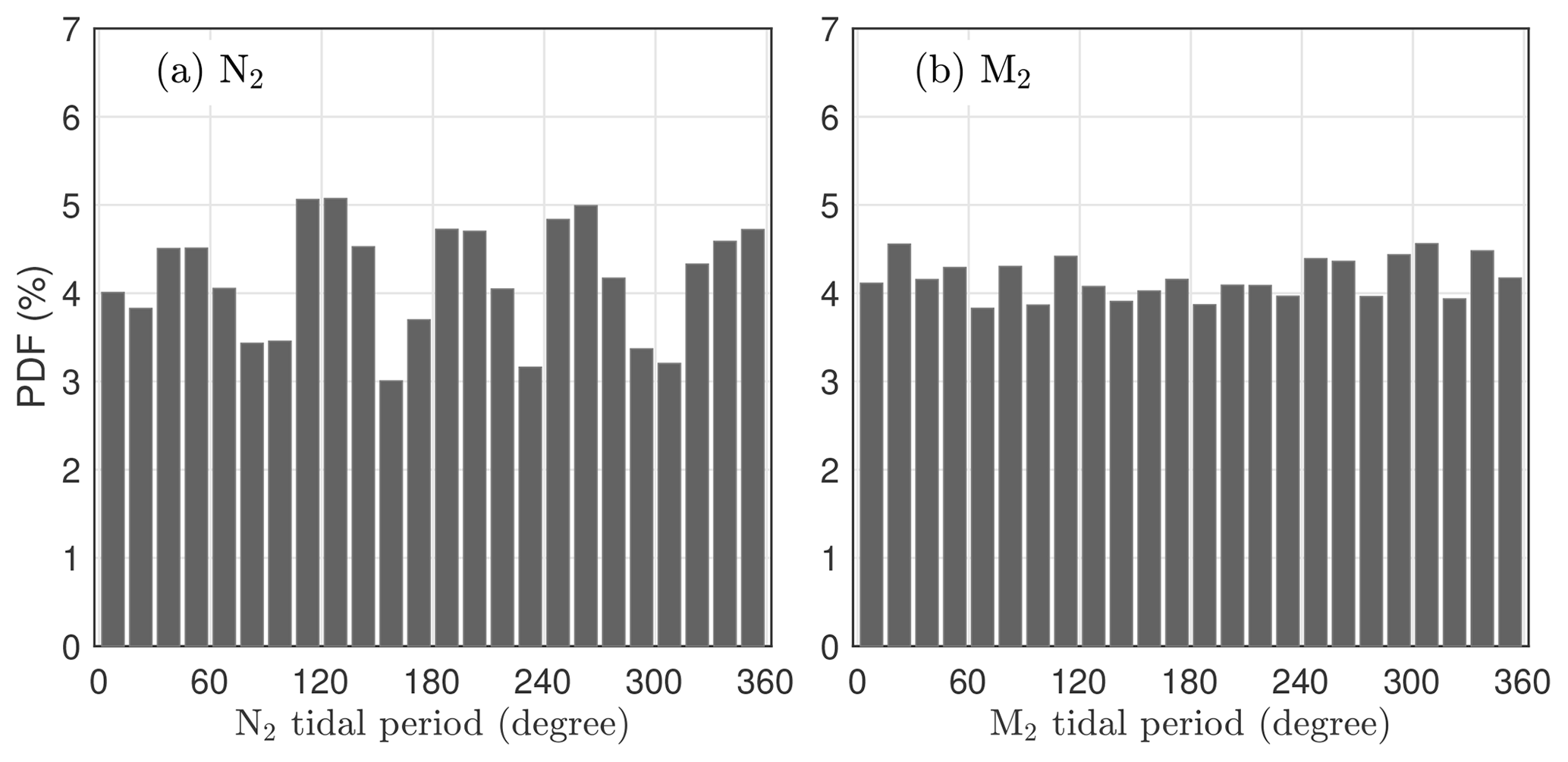
Figure 2Histograms of the phase lags of the satellite SSH data over one N2 (a) and M2 (b) tidal period. This example is for one 160 km by 160 km window centered at 15∘ N, 160∘ W. There are about 7.84×10⁴ SSH measurements in this window. From their observation times, the phase lags with respect to N2 and M2 are calculated.
2.2 Plane wave analysis
The core technique of our mapping procedure is plane wave analysis. By this method, internal tides are determined by fitting horizontal plane waves in one given fitting window (160 km by 160 km in this study), in contrast to harmonic analysis at one single site. This method has been described in detail in our previous studies (Zhao and Alford, 2009; Zhao, 2014; Zhao et al., 2016). For each tidal constituent, there may be multiple internal tides of arbitrary propagation directions at each site, due to their multiple source regions and long-range propagation. Plane wave analysis can resolve these internal tides by propagation direction. We will fit five mode-1 N2 internal tidal waves at each site. Our five-wave representor follows
where x and y are the east and north Cartesian coordinates, t is time, and ω and k are the frequency and horizontal wavenumber of the target internal tides, respectively. Three parameters need to be determined for each internal tidal wave: amplitude A, phase ϕ, and direction θ. To determine one wave, the amplitude and phase of a single plane wave are determined by the least-squares fit in each compass direction (with 1∘ increment). When the resulting amplitudes are plotted as a function of direction in polar coordinates, an internal tidal wave appears to be a lobe. The direction of the first wave is thus determined from the biggest lobe. Thus, the amplitude A, phase ϕ, and propagation direction θ of one internal tidal wave are determined. Afterward, its signal is predicted and subtracted from the original data, which removes the wave itself and its side lobes. This procedure can be repeated to extract an arbitrary number of waves one by one. The resulting internal tidal waves are sorted with descending amplitudes.
The frequency (ω) and horizontal wavenumber (k) of the target internal tides are needed in plane wave analysis. The M2 and N2 tidal periods (equivalent to frequencies) are from the Moon's orbital motion around the Earth (Doodson, 1921; Pawlowicz et al., 2002). They are 12.4206 and 12.6583 h, respectively. The local phase speed (equivalent to wavenumber) of the target internal tides is theoretically determined from the World Ocean Atlas 2018 (WOA18) (Boyer et al., 2018). The WOA18 provides climatological hydrographic profiles on a spatial grid of 0.25∘ latitude by 0.25∘ longitude. Ocean depth is based on the 1 arcmin topography database constructed using in situ and satellite measurements (Smith and Sandwell, 1997). For a given ocean depth and stratification profile, the vertical structures and eigenvalue speeds of internal tides are obtained by solving the Sturm–Liouville equation (Gill, 1982; Chelton et al., 1998; Kelly, 2016):
subject to free-surface and rigid-bottom boundary conditions, where N(z) is the buoyancy frequency profile and c is the eigenvalue speed. The phase speed cp can be calculated from the eigenvalue speed following
where ω and f are the tidal and inertial frequencies, respectively. Note that the phase speed is a function of longitude and latitude (Zhao et al., 2016).
2.3 Mapping procedure
Our three-step mapping procedure consists of two rounds of plane wave analysis and a spatial two-dimensional (2D) bandpass filter in between (Zhao, 2020, 2021, 2022a, b). In this paper, the mapping process is illustrated by showing intermediate results in Fig. 3. An interested reader is referred to the above papers for more details.
In step 1, mode-1 N2 internal tides are mapped by plane wave analysis as described above. The N2 internal tides are mapped from along-track SSH data onto a spatially regular grid. In this paper, our fitting window is chosen to be 160 km by 160 km, consistent with wavelengths of mode-1 N2 internal tides. The resulting N2 internal tides are at a 0.2∘ longitude by 0.2∘ latitude grid. At each grid point, five mode-1 N2 internal tidal waves of arbitrary propagation directions are determined. The vector sum of these five waves gives the internal tide solution. Figure 3a shows the mode-1 N2 internal tide field obtained in this step. It gives obvious internal tide signals (e.g., around the Hawaiian Ridge) but the non-tidal noise is high. In step 2, the spatially regular N2 internal tide field is cleaned by a 2D bandpass filter in overlapping 850 km by 850 km windows. The N2 internal tide field is first converted to the 2D wavenumber spectrum by Fourier transform. The spectrum is truncated to [0.8, 1.25] times the local wavenumber. The truncated spectrum is converted back to the internal tide field by inverse Fourier transform. Figure 3b shows the cleaned N2 internal tide field. Now the N2 internal tide signals are much cleaner. However, Fig. 3b cannot resolve multiple internal tidal waves yet. In step 3, plane wave analysis is called again to decompose the filtered internal tide field into five internal waves of arbitrary propagation directions. The second-round plane wave analysis is the same as the first-round plane wave analysis, except that the input is the filtered internal tide field in step 2. In the end, the resulting five waves are saved with their respective amplitudes, phases, and directions. Figure 3c shows the five-wave superimposed internal tide field. It is very similar to Fig. 3b because this step only decompose the internal tide field. The five-wave decomposition allows us to separate internal tides of different propagation directions. They will be used to extract long-range internal tidal beams in the ocean (Sect. 3).
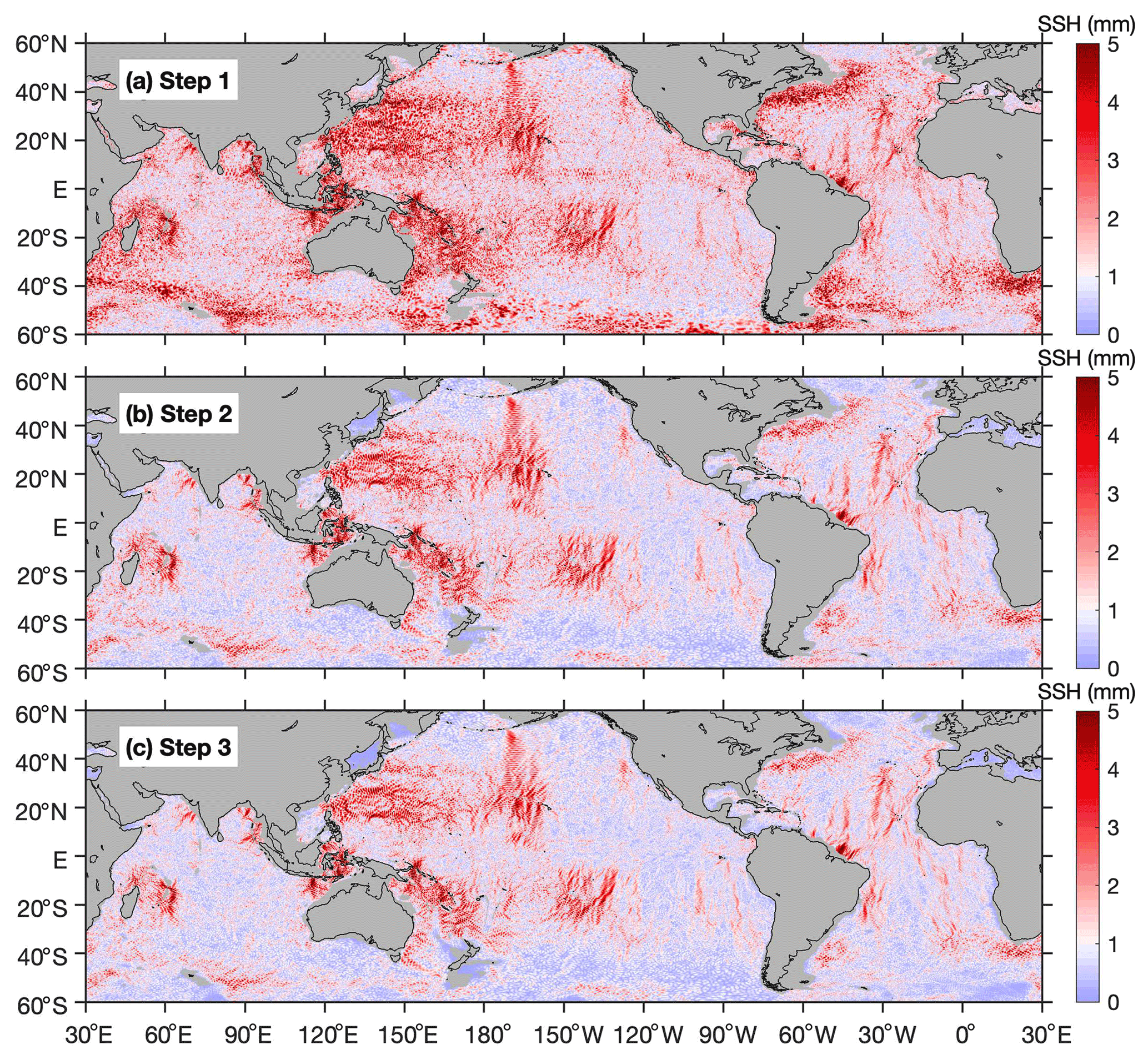
Figure 3The three-step mapping procedure. (a) Mode-1 N2 internal tides are obtained by the first-round plane wave analysis. (b) Mode-1 N2 internal tides are cleaned by 2D bandpass filtering. (c) Mode-1 N2 internal tides are decomposed by the second-round plane wave analysis. Shown here is the five-wave superposed amplitude.
2.4 N2 and M2 internal tides
We map both the mode-1 N2 and M2 internal tides following the same three-step procedure. They are constructed from the same satellite altimetry data but using their respective wave parameters (frequency and wavenumber). Figure 4 shows the resulting N2 and M2 internal tide fields. Internal tides in shallow waters (< 1000 m) are discarded. The new M2 internal tides are almost identical to those obtained in previous studies using slightly different satellite data (Zhao, 2022b). Here we find that the N2 and M2 internal tides have similar spatial patterns and that the N2 amplitudes are about 20 % of the M2 amplitudes. The largest N2 amplitudes are about 5 mm, compared to 20–30 mm for M2 internal tides. To account for this factor, their color map ranges are different by a factor of 5. Figure 4 gives SWOT ground tracks in its 1 d fast-repeating phase (green lines). It shows that strong mode-1 N2 internal tides occur under some SWOT swaths, for example, those off the California coast, in the New Caledonia region, in the western North Pacific, and on the Amazon continental shelf. In these regions, the N2 internal tides cannot be neglected in the study of sub-mesoscale dynamics. Conversely, the upcoming SWOT data also offer a great opportunity to explore N2 internal tides.
We have examined the possible cross talk between the N2 and M2 internal tides in our mapping procedure. We map N2 internal tides using two different data sets. The first is the original satellite altimetry SSH data set (Sect. 2.1). The second is the M2-corrected data set. In other words, the M2 internal tides are predicted using our empirical model and subtracted from the original data. We find that the resulting N2 internal tides from the two data sets are almost the same. The variance of their differences is < 1 % that of the N2 internal tides. Likewise, we map M2 internal tides using both the original and N2-corrected data sets and find that the impact of N2 on M2 is negligible. Our analysis reveals that the N2 and M2 internal tides do not cross talk in our mapping method. This is because the 27-year-long satellite data from 1993 to 2019 are sufficient long to unambiguously separate the N2 and M2 tidal constituents (about 14 min apart).
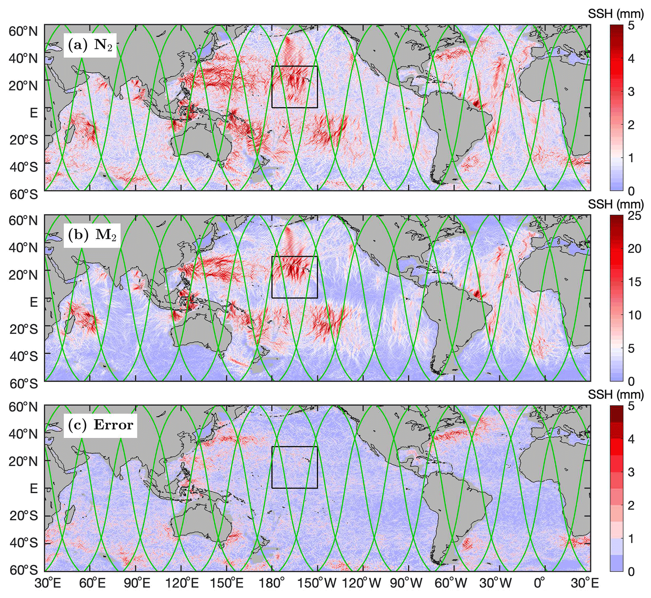
Figure 4Internal tides and model errors. Shown are their SSH amplitudes. (a) N2. (b) M2. N2 and M2 have similar spatial patterns. The N2 amplitudes are about 20 % of the M2 amplitudes. (c) Errors. The model errors are obtained by mapping internal tides with a tidal period of 12.6074 h (Fig. 5) using the same satellite altimetry data and following the same mapping procedure. Green lines denote SWOT ground tracks in the fast-repeating phase. The mean SSH amplitudes in the black box are given in Fig. 5.
2.5 Model errors
Model errors in our N2 and M2 internal tide models are estimated using background internal tides. In contrast to N2 and M2 internal tides, which are mapped using tidal periods of 12.6583 and 12.4206 h, respectively, background internal tides are mapped using the same satellite altimetry data but for tidal periods between N2 and M2. Specifically, we map 13 sets of background internal tides using 13 different tidal periods that are linearly interpolated between N2 and M2 (Fig. 5). The other mapping parameter, wavenumber (equivalently phase speed), can be obtained using Eq. (3). The same strategy has previously been employed to estimate barotropic tide errors. For example, Ray and Susanto (2016) study the fortnightly tidal cycles (MSf and Mf) of tidal mixing using satellite sea surface temperature data. Zaron et al. (2023) study the fortnightly variability in Chl a using satellite sea surface color data. In both studies, tidal errors are estimated using signals at fake or false tidal frequencies near the real tidal constituents.
We thus obtain 13 background internal tides in the central Pacific (Fig. 4c, box). Their regional mean SSH amplitudes in this region are 0.8 ± 0.1 mm, compared to 1.66 and 7.75 mm for N2 and M2 (Fig. 5). Note that the SSH amplitudes of the 13 background internal tides are almost the same, showing no significant tidal cusps around the N2 or M2 internal tides. In addition, we have calculated the correlation coefficients among these 15 sets of internal tides (including N2 and M2). All correlation coefficients are < 0.05, suggesting that these background internal tides are independent of each other and of the N2 and M2 internal tides. In other words, background internal tides are signals we obtain where there are no tidal constituents. We suggest that the model errors in N2 and M2 can be represented by background internal tides. In this study, we pick one tidal period (12.6074 h) for a global run to obtain background internal tides (model errors), considering that a global run is time-consuming. Figure 4c gives the resulting background internal tides (model errors). It reveals that model errors are large in regions of strong mesoscale motions because model errors are mainly leaked mesoscale signals. Figure 4 shows that the N2 internal tides are noisier than M2 because the small-amplitude N2 internal tides are easily affected by model errors. On a global average, the error variance is about 25 % of the N2 variance, and only 1 % of the M2 variance.
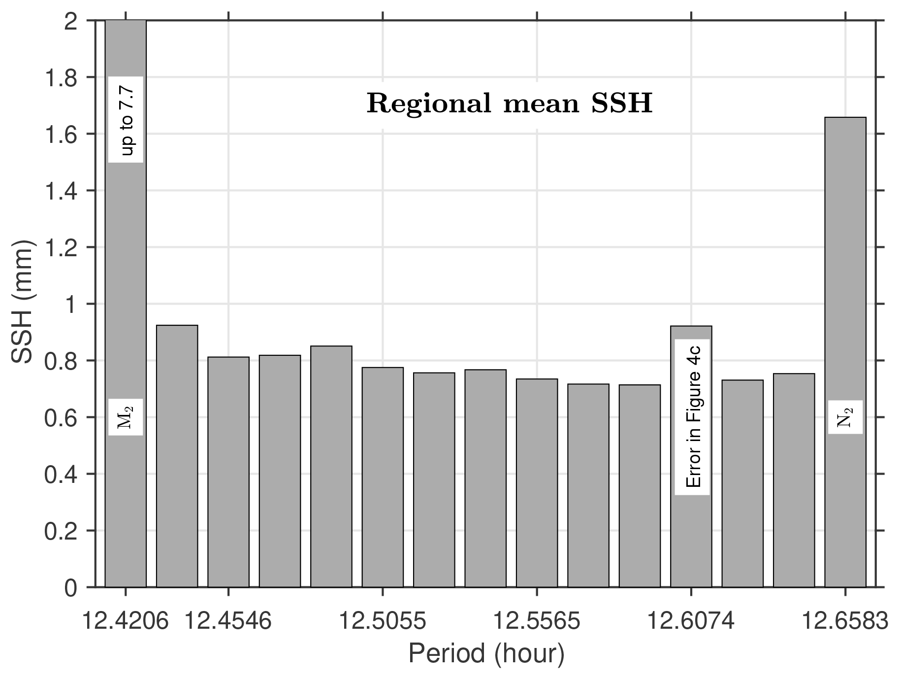
Figure 5Histogram of regional mean SSH amplitudes. In the central Pacific Ocean (0–30∘ N, 180–150∘ W), 15 sets of internal tides are determined using the same satellite data and following the same procedure. They are mapped using their respective periods and wavenumbers. Tidal periods of the 13 sets of background internal tides are linearly interpolated between N2 and M2.
2.6 Model evaluation
Our N2 and M2 internal tide models are evaluated using independent satellite SSH data collected in 2020 and 2021. For each SSH measurement of known time and location, the internal tide signal is predicted using the model under evaluation and subtracted from the SSH measurement. Variance reduction is the variance difference before and after the internal tide correction. The variance reductions for all SSH measurements are binned into 2∘ by 2∘ boxes. The global map of N2 variance reduction is shown in Fig. 6a. The M2 internal tide model is evaluated in the same way and shown in Fig. 6b. Note that the color map ranges for N2 and M2 differ by a factor of 25, that is, the square of the factor of their amplitudes.
In the evaluation, the true N2 internal tides (variance ) in the model will remove the N2 internal tides in the independent data, leading to positive variance reduction, while the model errors (variance ) will increase the variance of the independent data, leading to negative variance reduction. Together, we obtain positive variance reduction where , and negative variance reduction where . Figure 6a shows positive variance reduction in the global ocean, suggesting that the true N2 internal tides are greater than model errors. In particular, in regions of strong N2 internal tides such as the Hawaiian Ridge and the Amazon continental shelf, patches of positive variance reduction are observed because the strong N2 internal tides can overcome model errors, while negative variance reduction usually occurs in regions of weak N2 internal tides such as the eastern equatorial Pacific and the Southern Ocean. The regions of strong mesoscale motions are dominated by negative variance reduction, where weak N2 internal tides are overwhelmed by large model errors (Fig. 4c). For comparison, Fig. 6b shows that the M2 internal tide model causes positive variance reduction throughout the global ocean, except for regions of strong mesoscale motions or strong temporal variation (Zhao, 2021). This is because the strong M2 internal tides are almost always greater than the model errors . In summary, our N2 internal tide model can reduce variance in some regions, although the N2 SSH amplitudes are just a few millimeters.
We further examine the relation between the N2 variance reduction shown in Fig. 6a and the variance difference between the N2 model and the model error. Figure 6c and d give the N2 model variance and the error variance that are computed from Fig. 4a and c, respectively. Note that the N2 model variance σ2 contains both true N2 internal tides and errors . Under the condition that the N2 variance is greater , we should have . We thus calculate the variance difference and show the global map in Fig. 6e. To test this relation, we calculate the variance difference for m ranging from 0.5 to 3.5 with a step of 0.1. For each resulting variance difference map (e.g., Fig. 6e), we calculate its correlation coefficient with the N2 variance reduction (Fig. 6a). We get the best spatial correlation when the factor m is 2, consistent with our theoretical analysis. Note that all the above analyses are based on the 2∘ by 2∘ binned values. Figure 6f shows the mask region where the N2 model variance is greater than twice the error variance, indicating regions where the N2 model can be used to make internal tide correction. The mask covers regions of strong N2 and M2 internal tides such as the Hawaiian Ridge, the area off the California coast, the Amazon continental shelf, the western North Pacific, and New Caledonia.
We next examine the performance of the N2 and M2 internal tide models in making internal tide correction for SWOT. In Fig. 6, the green lines denote the SWOT ground tracks in its daily fast-repeating phase. We interpolate the N2 and M2 variance reductions onto the SWOT ground tracks (neglecting its swath) and calculate the along-track mean variance reductions. For N2, the mean variance reductions in and outside the mask region are 0.73 and −0.25 mm2, respectively. The negative variance reduction suggests that the N2 model does not work well outside the mask region. Fortunately, the N2 model can make internal tide correction in the mask region where the N2 internal tides can overcome model errors. The variance reductions caused by the N2 model seem small, but keep in mind that (1) internal tides and sub-mesoscale motions both have millimeter-scale SSH amplitudes and (2) internal tides are much stronger in their source regions. For M2, the along-track mean variance reductions in and outside the mask region are 25.6 and 2.5 mm2, respectively. They suggest that the M2 model performs well both in and outside the mask region because the M2 internal tides dominate errors throughout the global ocean.
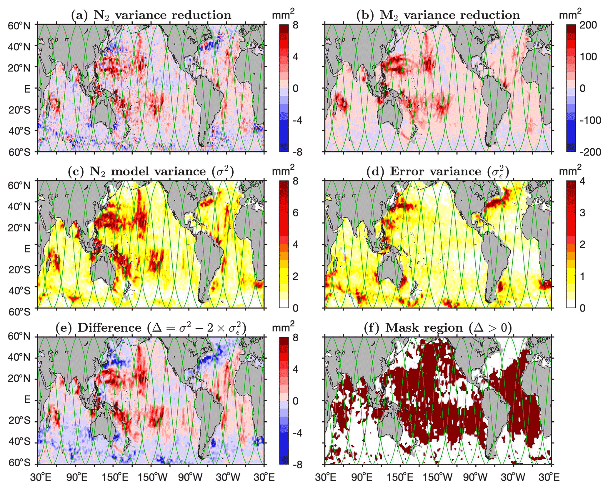
Figure 6Model evaluation. Internal tide models are evaluated using independent altimetry data in 2020 and 2021. Shown are variances or variance reductions binned in 2∘ by 2∘ boxes. (a) N2. (b) M2. (c) Variance of the N2 model. (d) Variance of the model error. (e) Difference between the N2 model variance and twice the error variance. The factor of 2 is chosen to obtain the best spatial correlation between (a) and (e). (f) Mask region where the model variance is greater than twice the error variance, which implies the true N2 variance is greater than the error variance. The mask indicates regions where the N2 model can be used to make internal tide correction. Green lines denote SWOT ground tracks in the fast-repeating phase.
3.1 Global distribution
Our mode-1 N2 model reveals that N2 internal tides are widespread in the global ocean (Fig. 4a). In the Indian Ocean, they are observed in the Arabian Sea, the Bay of Bengal, and the Madagascar–Mascarene region. In the Pacific Ocean, N2 internal tides occur in regions such as the French Polynesian Ridge, the Hawaiian Ridge, the Indonesian seas, the western South Pacific, and the western North Pacific. In the Atlantic Ocean, N2 internal tides appear in regions including the Azores region, the Amazon shelf, the Bay of Biscay, and the Vitória–Trindade Ridge. Our M2 model reveals that mode-1 M2 internal tides are observed in the same regions (Fig. 4b). The N2 and M2 internal tides have similar spatial patterns, but the N2 amplitudes are about 20 % of the M2 amplitudes. To further quantify their relation, we give in Fig. 7a the scatterplot of the N2 and M2 SSH amplitudes. It shows that the N2 and M2 amplitudes largely follow the diagonal line with a ratio of 5. Their correlation coefficient is 0.69 (R in MATLAB function corrcoef).
We extract the N2 and M2 barotropic tides from TPXO.8 (Egbert and Erofeeva, 2002) and show them in Fig. 8. We find that the N2 and M2 barotropic tides have similar spatial patterns and that the N2 amplitudes are about 20 % of the M2 amplitudes. We examine the relation between the N2 and M2 barotropic tides as well. Figure 7b shows the scatterplot of the N2 and M2 barotropic amplitudes. It shows that N2 and M2 have a very tight relation, with a correlation coefficient of 0.96. Egbert and Ray (2003) show that the M2 and N2 barotropic-to-baroclinic energy conversion maps have similar spatial patterns and that their amplitudes differ by a factor of 25 (see their Fig. 1). The N2 and M2 relation (spatial pattern and amplitude ratio) is the same for both barotropic and baroclinic tides. Because N2 and M2 have close tidal periods (12.6583 and 12.4206 h), their generations over the same topographic features should be the same (distinguishing their slight differences may improve our understanding of internal tide dynamics in the future). In addition, it is reasonable that the N2 and M2 internal tides have a relatively weak relation (Fig. 7a) because the long-range propagation of internal tides is affected by an inhomogeneous ocean environment.
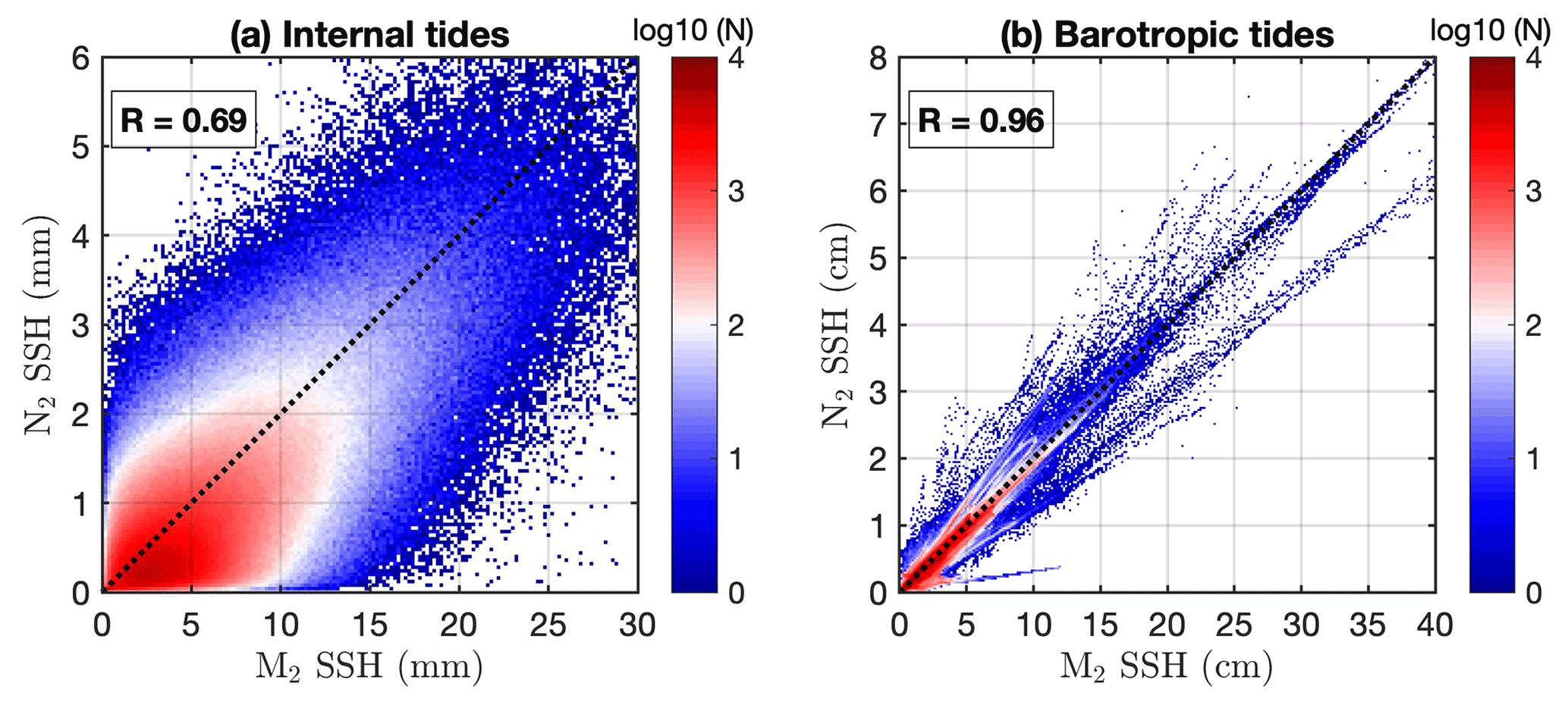
Figure 7Scatterplots of N2 and M2 amplitudes. (a) Internal tides. (b) Barotropic tides. Shown is the data density on a logarithmic scale. Their correlation coefficients are calculated. For both the barotropic and internal tides, the N2 amplitudes are about 20 % of the M2 amplitudes.
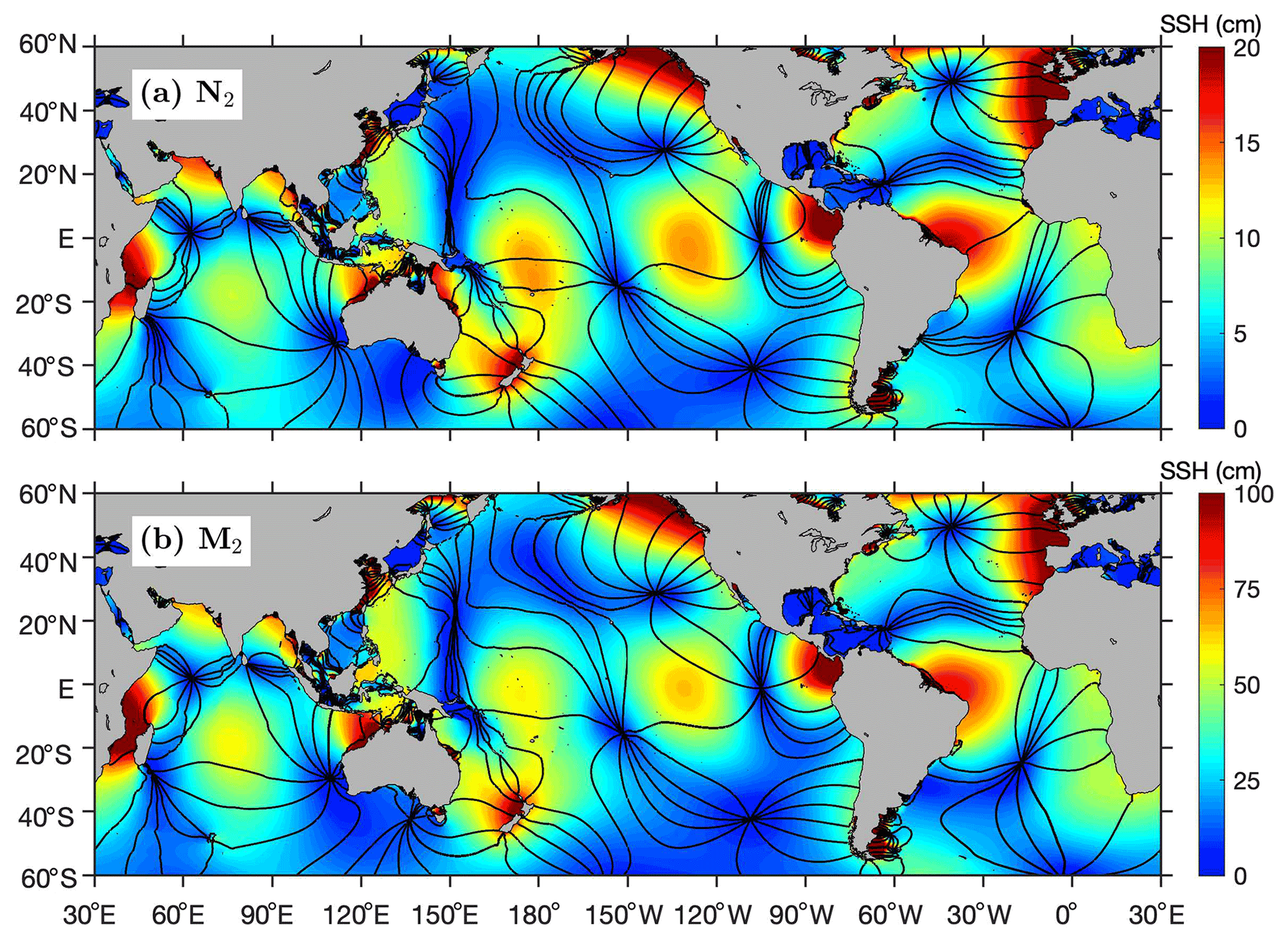
Figure 8N2 and M2 barotropic tides from TPXO.8. Colors show amplitudes. Black lines show co-phase charts at 30∘ intervals. N2 and M2 have similar spatial patterns, and the N2 amplitudes are about 20 % of the M2 amplitudes.
3.2 Long-range beams
In this section, we study the long-range mode-1 N2 internal tidal beams. We have fitted five mode-1 N2 internal tidal waves at each grid point by plane wave analysis. Taking advantage of the five-wave fits, we can decompose the N2 internal tide field into the northward (0–180∘ counterclockwise from due east) and southward (180–360∘) components by propagation direction. Each component contains internal tidal waves with propagation directions falling in the given range (Fig. 9). The decomposed components clearly show well-defined long-range N2 internal tidal beams, which are characterized by larger amplitudes and cross-beam co-phase lines (not shown here for clarity; see Figs. 10 and 11). There are numerous long-range N2 internal tidal beams, which radiate from the strong generation sites mentioned above. For example, northward N2 beams are observed to originate from the French Polynesian Ridge, the Macquarie Ridge, and the Amazon shelf. Southward N2 beams are observed to originate from the Andaman Islands, the Lombok Strait, the Hawaiian Ridge, the French Polynesian Ridge, the Mendocino Ridge, and the Azores, among others. Note that the M2 long-range internal tidal beams have been well studied in previous studies (Zhao et al., 2016, Fig. 5 therein). To avoid repetition, the M2 internal tidal beams are not shown here. Together, we observe that the N2 and M2 internal tides have similar long-range beams. In this study, we examine two long-range internal tidal beams as examples.
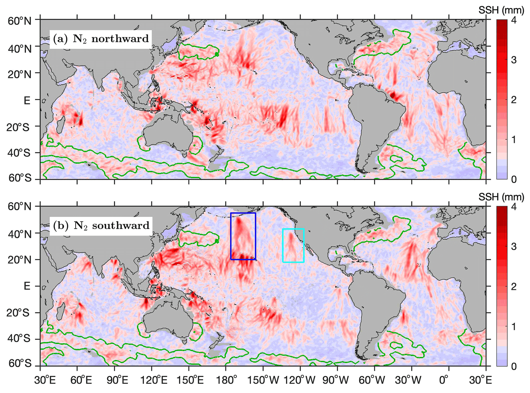
Figure 9Decomposed N2 internal tide fields. (a) Northward component (directional range: 0–180∘ counterclockwise from due east). (b) Southward component (directional range: 180–360∘). Internal tides in shallow waters (< 1000 m) are discarded. Green contours indicate regions of strong mesoscale motions, where the N2 internal tides are overwhelmed by errors (see Fig. 6e).
First, we examine the southward internal tides from the Amukta Pass, Alaska. The M2 long-range beam from Amukta Pass has been studied recently (Zhao, 2022b). Figure 10a shows the southward N2 internal tides in the central North Pacific (Fig. 9b, blue box). For comparison, the southward M2 internal tides are shown in Fig. 10b. Both tidal constituents can travel from the Aleutian island chain to the Hawaiian Ridge over 3000 km away. Their propagation directions are about −78∘ from due east. The black lines in Fig. 10 show the 0 and 180∘ co-phase charts. Figure 10c shows their phase difference, which increases with propagation because N2 internal tides travel faster than M2 internal tides according to Eq. (3). In the propagation, their phase difference increases with propagation. Along the dashed line from source (52.6∘ N, 189∘ E) to far field (26∘ N, 195∘ E), their phase difference increases from 65 to 305∘. The overall phase change is 240∘. It takes about 18 tidal cycles for the N2 and M2 internal tides to travel along the path.
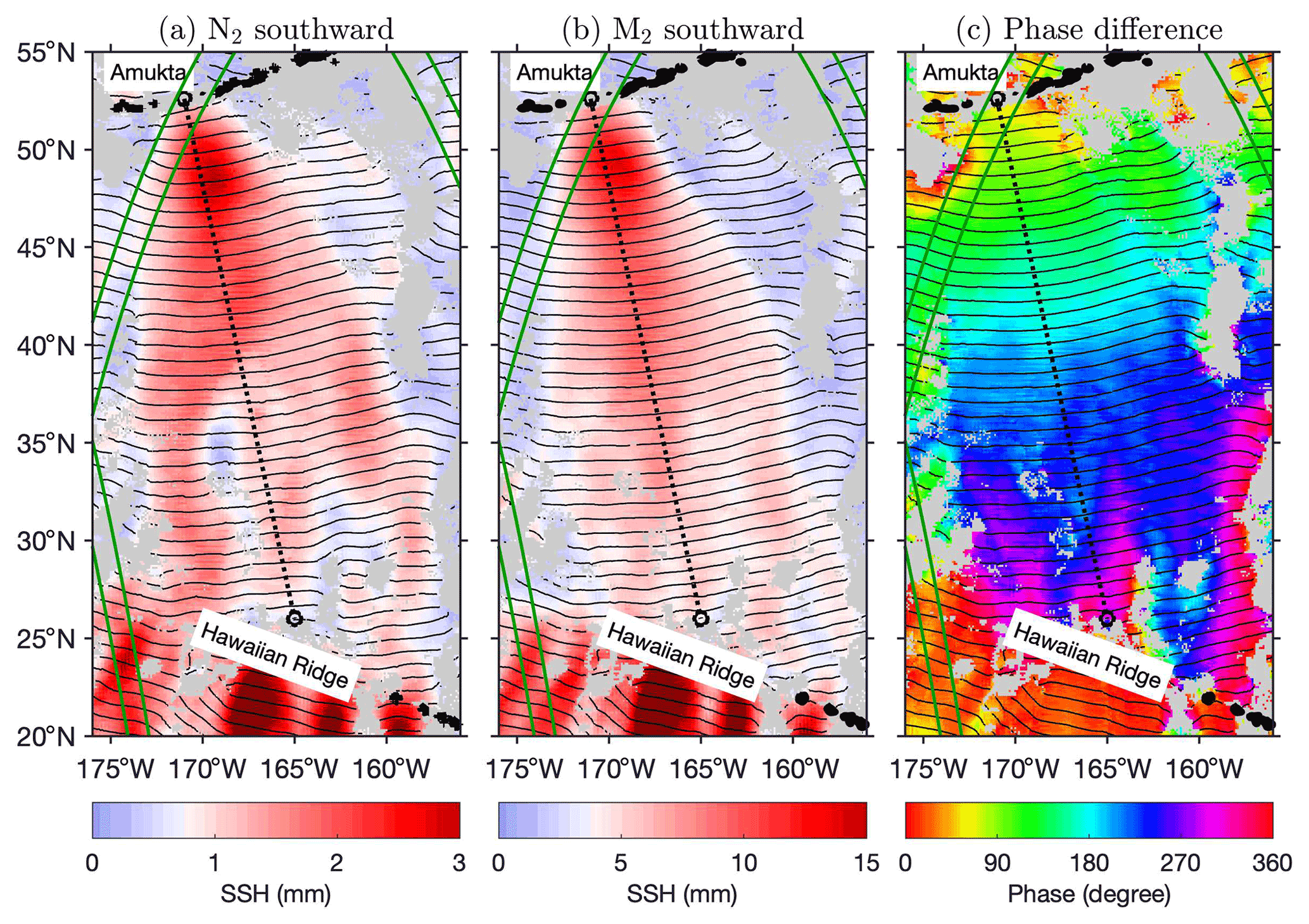
Figure 10Southward (180–360∘) internal tides from Amukta Pass, Alaska. (a) N2 internal tides. (b) M2 internal tides. Black contours show the 0 and 180∘ co-phase lines. Intervals between two neighboring co-phase lines are half wavelengths. (c) Phase difference between N2 and M2. Black contours show the M2 co-phase lines as in (b). Weak internal tides are discarded (M2 < 1 mm; N2 < 0.2 mm). Both N2 and M2 internal tides can propagate over 3000 km from the Aleutian Ridge to the Hawaiian Ridge. Along the 3000 km long path (dashed lines), their phase difference increases from 65 to 305∘. Green lines denote the 120 km wide SWOT swaths in the fast-repeating phase.
Figure 11 shows southward internals tides in the region off the California coast (Fig. 9b, cyan box). This region is chosen for a detailed investigation because it contains one site for the SWOT calibration/validation field campaign. The green lines in this figure indicate the SWOT swaths in its fast-repeating phase (Wang et al., 2022). The crossover region of the ascending and descending swaths is the SWOT calibration/validation site. This region is dominated by the southward internal tides from the Mendocino Ridge. Note that this region is also affected by internal tides in other propagation directions (Zhao et al., 2019). Additionally, there are southwestward internal tides from the Monterey Bay. The two internal tidal beams intersect around the SWOT campaign site. As explained earlier, our N2 model can make internal tide correction for SWOT. Figure 11 shows that N2 and M2 internal tides are very similar, although the N2 fluxes are much weaker. Both N2 and M2 beams can be tracked from 40 to 20∘ N for > 2000 km. They both bifurcate around 32∘ N near Fieberling seamounts (32.5∘ N, 232.3∘ E) for unknown reasons. The dashed line delineates the beam from 40.3 to 22∘ N along 128∘ W. This line is about 2000 km long. Along this line, the N2 and M2 phase difference increases from 40 to 160∘ over about 14 M2 or N2 tidal cycles.
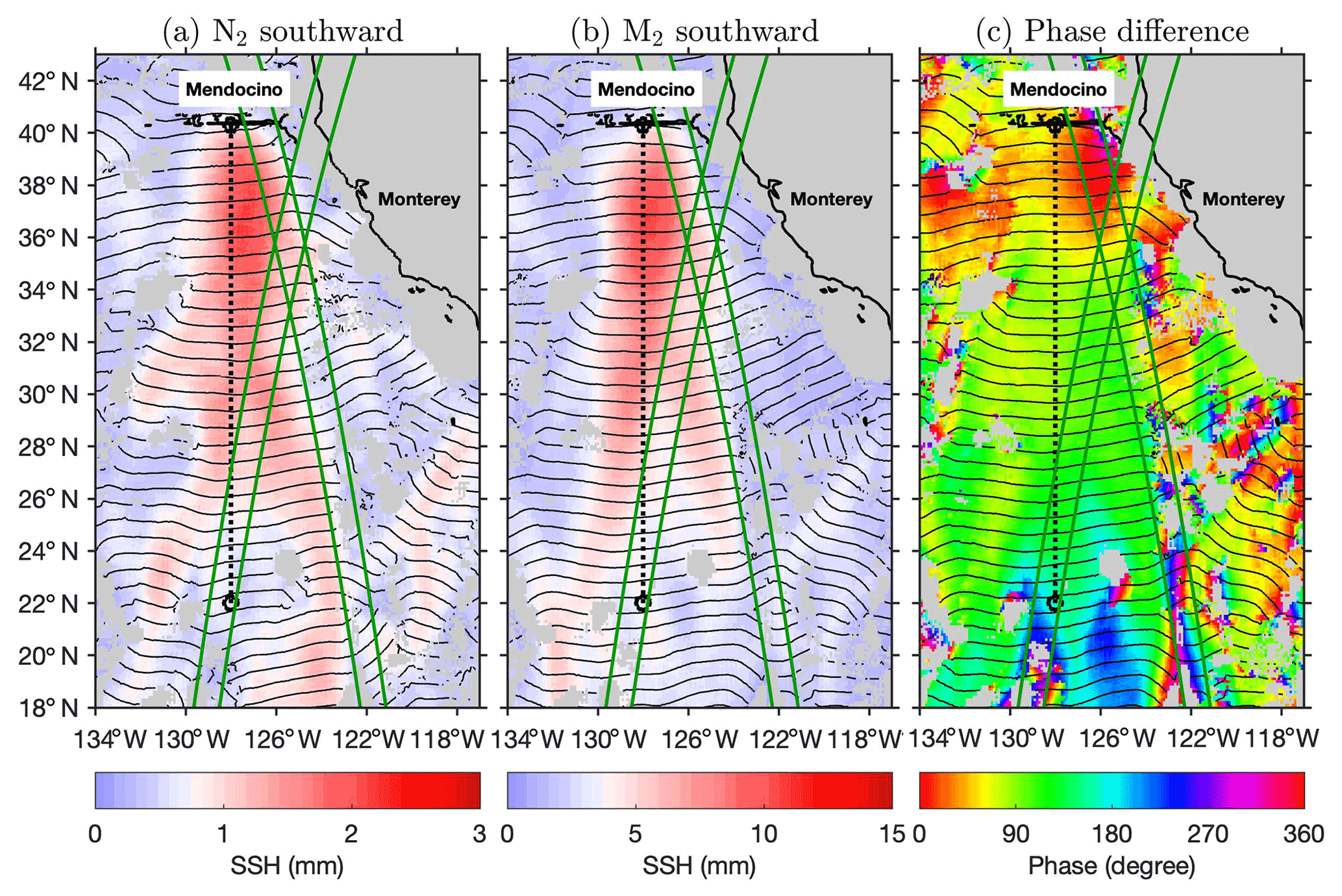
Figure 11Southward (180–360∘) internal tides off the US west coast. (a) N2 internal tides. (b) M2 internal tides. Colors show SSH amplitudes. Black contours indicate the 0 and 180∘ co-phase lines. Southward internal tides are mainly from the Mendocino Ridge. Weak internal tides are discarded (M2 < 1; N2 < 0.2 mm). Internal tides in shallow waters (< 1000 m) are discarded. (c) Phase difference between N2 and M2. Green lines denote two 120 km wide SWOT swaths in the fast-repeating phase.
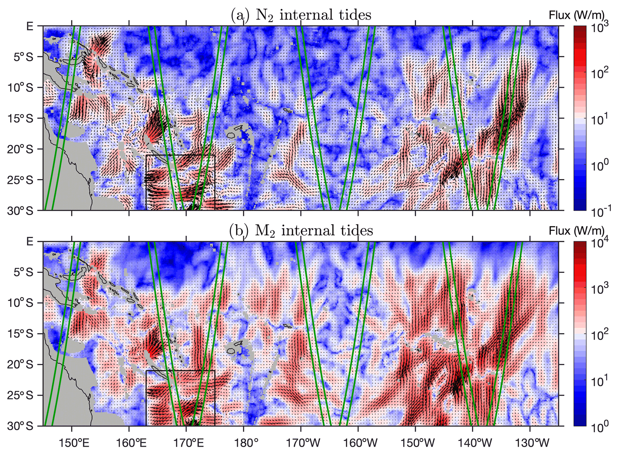
Figure 12Internal tide energy fluxes in the western South Pacific. (a) N2 internal tides. (b) M2 internal tides. Colors show flux magnitudes and black arrows show flux vectors. Internal tides in shallow waters (< 1000 m) are discarded (gray shading). Green lines indicate SWOT swaths in the fast-repeating phase.
3.3 Energy and energy flux
We calculate the depth-integrated energy flux of mode-1 N2 internal tide from their SSH amplitudes and a transfer function (Fn). The transfer function is calculated using the WOA18 climatological hydrography and the Sturm–Liouville equation (Zhao and Alford, 2009; Zhao et al., 2016). The same calculation method has also been derived by Geoffroy and Nycander (2022). In this study, we follow our method (previously for mode-1 M2 internal tides) to obtain the transfer function for mode-1 N2 internal tides. It is a function of ocean depth, tidal frequency, mode number, latitude, and stratification. The transfer functions for N2 and M2 are very close because their tidal periods are close. At each grid point, we thus obtain five energy fluxes for the five internal tidal waves following , where A is the SSH amplitude. The vector sum of the five energy fluxes gives the final energy flux at this site. In this study, we compare the N2 and M2 internal tide energy fluxes in two regions. An interested reader can examine other ocean regions. We show that their energy fluxes have similar spatial patterns. The results show that the mode-1 N2 internal tides can be observed by satellite altimetry, although they are much weaker than the M2 internal tides. Following the same procedure, we have computed the depth-integrated internal tide energies from SSH amplitudes. The globally integrated area-weighted energies for the N2 and M2 internal tides are 1.8 and 30.9 PJ, respectively. The N2-to-M2 ratio is about 5.8 %, larger than the theoretical value of 4 % because N2 contains larger error variance. As explained earlier, the error variance is about 25 % of the N2 variance but only 1 % of the M2 variance.
Figure 12 shows the N2 and M2 energy fluxes in the western South Pacific. In this study, it is trimmed to 30∘ S–0∘, 145∘ E–125∘ W. Colors show flux magnitudes, and black arrows show flux vectors. This region is chosen because (1) it features various topographic obstacles such as mid-ocean ridges and island chains and (2) the New Caledonia region is one site for SWOT calibration/validation field experiments (Bendinger et al., 2023). There are numerous N2 and M2 internal tidal beams in this region. They are dominantly generated over topographic features. For example, N2 and M2 internal tidal beams radiate from many straits surrounding the Coral Sea (Tchilibou et al., 2020). The internal tidal beams can be in any horizontal propagation direction. From the French Polynesian Ridge, internal tides mainly propagate southward and northward. From the Kermadec Arc and New Caledonia, the outgoing internal tidal beams usually travel eastward or westward. The energy fluxes of N2 and M2 internal tides have similar spatial patterns. Figure 12 shows seven SWOT swaths in this region (green lines). Among them, the two swaths in the New Caledonia region (black box) overlap with strong N2 internal tides whose contribution cannot be neglected. In addition, the two swaths cross the French Polynesian Ridge, where one should pay an attention to N2 and M2 internal tides in the study of mesoscale and sub-mesoscale processes.
Figure 13 shows the N2 and M2 energy fluxes in the North Atlantic Ocean (2∘S–53∘ N, 58–3∘ W). Figure 13 is in the same format as Fig. 12. Internal tides in this region have attracted much attention in recent years (Vic et al., 2018; Köhler et al., 2019; Löb et al., 2020). In particular, internal tides on the Amazon continental shelf have been intensively studied recently, partly because of the co-existence of internal tides and internal solitary waves (Egbert and Erofeeva, 2021; Tchilibou et al., 2022; Assene et al., 2023). Our satellite observation reveals that strong N2 and M2 internal tides occur around notable topographic features including the Mid-Atlantic Ridge, the Amazon continental shelf, the Azores region, the Bay of Biscay, the Canary Islands, and the Cabo Verde islands. The longest internal tidal beams for both N2 and M2 are the southward internal tidal beams from the Azores (Zhao, 2016; Köhler et al., 2019). The two beams can be tracked over 2000 km. In this region, there are four SWOT swaths in its fast-repeating phase, which overlap remarkable N2 and M2 internal tidal beams.
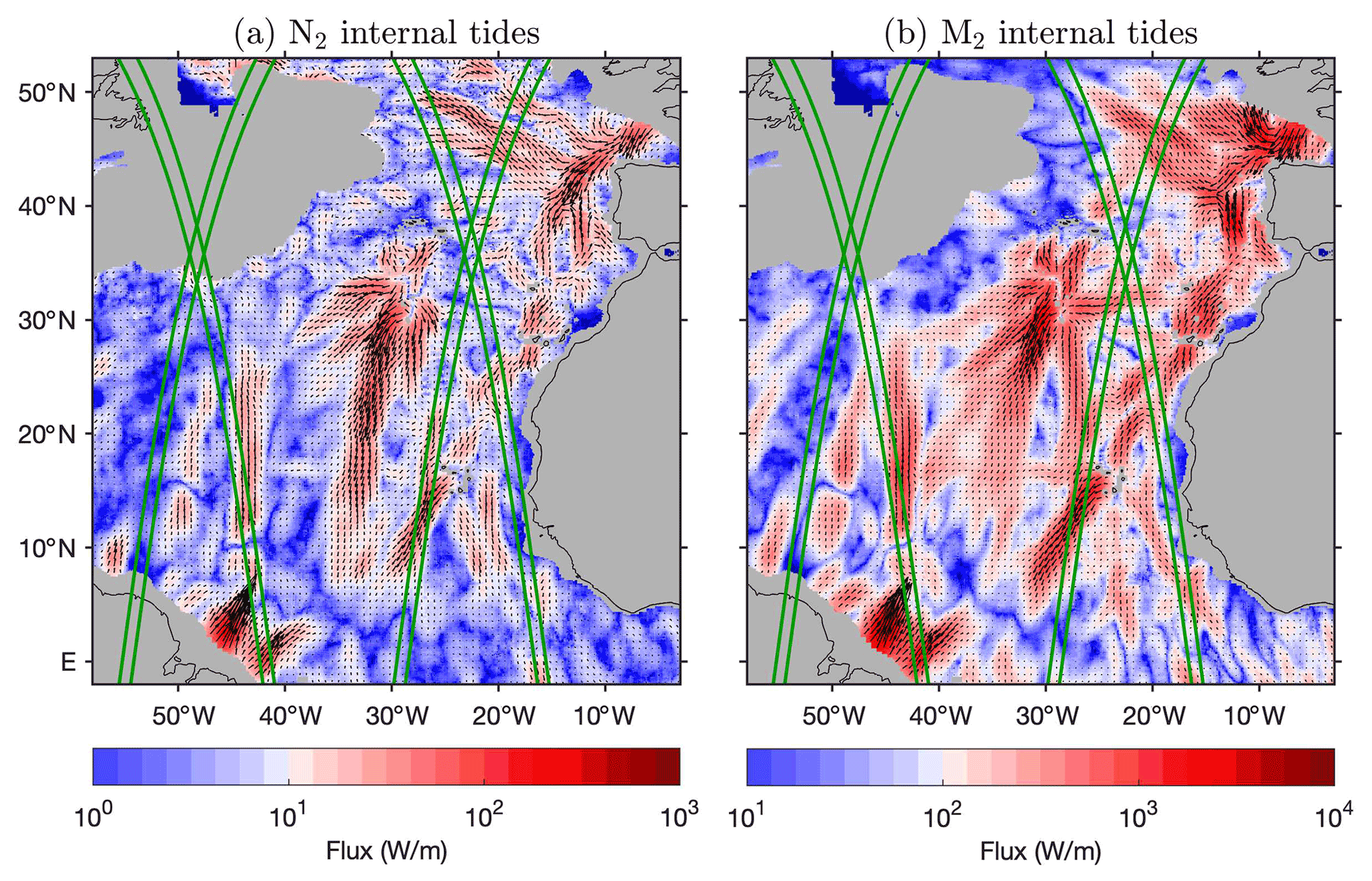
Figure 13As in Fig. 12 but for internal tide energy flux in the North Atlantic Ocean.
In this study, we constructed empirical models for mode-1 N2 and M2 internal tides from satellite altimetry. Among them, N2 is the larger lunar elliptical semidiurnal constituent and the fifth largest oceanic tidal constituent. It is induced by the Moon's elliptical orbit. Its amplitudes are about 20 % of the M2 amplitudes. The mode-1 N2 internal tides have sub-centimeter-scale SSH amplitudes. We can extract weak N2 internal tides because we use a larger altimetry data set and a newly developed mapping procedure. First, we use the multiyear multi-satellite altimetry data from 1993 to 2019. The combined data are about 100 satellite years long, which can significantly suppress non-tidal errors. Second, we extract mode-1 N2 internal tides by a three-step mapping procedure, which cleans internal tides using known frequency and wavenumbers of the target internal tide. In consequence, satellite altimetry can observe mode-1 N2 internal tides with millimeter-scale SSH amplitudes. Our N2 internal tide model is still noisy. Future improvements can be made with more and more satellite altimetry data becoming available.
We estimated errors in the N2 and M2 internal tide models using background internal tides. Specifically, background internal tides are mapped using the same altimetry data but for tidal periods between N2 and M2. In this study, we construct a global map of model errors using a tidal period of 12.6074 (N2 minus 3 min). The model errors are usually < 1 mm in the global ocean, with the global mean error being about 0.7 mm. Large errors usually occur in regions of strong mesoscale motions, since the model errors mainly come from the leaked mesoscale signals. On a global average, the error variance is about 25 % of the N2 model variance but only 1 % of the M2 model variance.
Our satellite observations revealed some basic features of the global N2 internal tides. We found that the N2 and M2 internal tides have similar spatial patterns and that the N2 amplitudes are about 20 % of the M2 amplitudes. Both features are determined by their barotropic counterparts. We found that both N2 and M2 internal tides can propagate hundreds to thousands of kilometers in the open ocean but at different phase speeds. We examined regional N2 internal tides and revealed rich information on their generation and propagation. We suggest that including N2 internal tides can better simulate the temporal variation in internal tide energetics with the lunar elliptical orbit.
Our N2 and M2 internal tide models have been evaluated using independent altimetry data in 2020 and 2021. The M2 model can cause variance reduction throughout the global ocean because the M2 internal tides dominate the model errors. In contrast, the N2 model can cause variance reduction in regions of strong N2 internal tides where they can overcome errors. We found that the N2 model performs well in regions where the N2 model variance is greater than twice the error variance, which means that the true N2 variance is greater than the error variance. We showed that the N2 and M2 models work well in the mask region along the SWOT fast-repeating tracks, which suggests that they can make internal tide correction for SWOT.
Last but not least, we demonstrated that our mapping technique can construct a reliable mode-1 N2 internal tide model using 100 satellite years of altimetry data. We have applied our mapping technique to the first baroclinic mode of other minor tidal constituents and higher baroclinic mode of other major tidal constituents and obtained clear internal tide signals. We have tried mapping mode-2 N2 internal tides around the Hawaiian Ridge (18–28∘ N, 185–205∘ E). However, the resulting model is noisy, as expected. In this region, the mean amplitude of mode-1 N2 internal tides is about 2.5 mm. The mean mode-2 N2 amplitude is estimated to be 1 mm, using a ratio of 2.5 from mode-1 and mode-2 M2 internal tides. The ∼ 1 mm mode-2 N2 internal tides cannot overcome the ∼ 0.7 mm noise. It is expected that the low-noise SWOT data along 120 km wide swaths will improve the observation of minor tidal constituents and higher baroclinic modes.
The satellite altimetry along-track data are from the Copernicus Marine Service (https://doi.org/10.48670/moi-00146, Satellite observations, 2020a). The satellite altimetry gridded data are from the Copernicus Marine Service (https://doi.org/10.48670/moi-00148, Satellite observations, 2020b). The SWOT orbit data are from the AVISO website (https://www.aviso.altimetry.fr/en/missions/current-missions/swot, last access: 18 September 2015). The World Ocean Atlas 2018 is produced and made available by NOAA National Oceanographic Data Center (https://www.nodc.noaa.gov/OC5/woa18/, last access: 1 May 2020). The mode-1 N2 internal tide model developed in this study is freely available (https://doi.org/10.6084/m9.figshare.23243633.v1, Zhao, 2023).
The author has declared that there are no competing interests.
Publisher’s note: Copernicus Publications remains neutral with regard to jurisdictional claims in published maps and institutional affiliations.
The author thanks Katsuro Katsumata, Clément Vic, and two anonymous referees for their constructive suggestions that have greatly improved this paper.
This research has been supported by the National Aeronautics and Space Administration (grant nos. NNX17AH57G and 80NSSC18K0771).
This paper was edited by Katsuro Katsumata and reviewed by Clément Vic and two anonymous referees.
Arbic, B. K.: Incorporating tides and internal gravity waves within global ocean general circulation models: A review, Prog. Oceanogr., 206, 102824, https://doi.org/10.1016/j.pocean.2022.102824, 2022. a
Assene, F., Koch-Larrouy, A., Dadou, I., Tchilibou, M., Morvan, G., Chanut, J., Vantrepotte, V., Allain, D., and Tran, T.-K.: Internal tides off the Amazon shelf Part I : importance for the structuring of ocean temperature during two contrasted seasons, EGUsphere [preprint], https://doi.org/10.5194/egusphere-2023-418, 2023. a
Bendinger, A., Cravatte, S., Gourdeau, L., Brodeau, L., Albert, A., Tchilibou, M., Lyard, F., and Vic, C.: Regional modeling of internal tide dynamics around New Caledonia: energetics and sea surface height signature, EGUsphere [preprint], https://doi.org/10.5194/egusphere-2023-361, 2023. a
Boyer, T. P., García, H. E., Locarnini, R. A., Zweng, M. M., Mishonov, A. V., Reagan, J. R., Weathers, K. A., Baranova, O. K., Paver, C. R., Seidov, D., and Smolyar, I. V.: World Ocean Atlas 2018, Tech. Rep., NOAA National Centers for Environmental Information, https://www.ncei.noaa.gov/archive/accession/NCEI-WOA18 (last access: 1 May 2020), 2018. a
Byun, D.-S. and Hart, D. E.: A monthly tidal envelope classification for semidiurnal regimes in terms of the relative proportions of the S2, N2, and M2 constituents, Ocean Sci., 16, 965–977, https://doi.org/10.5194/os-16-965-2020, 2020. a
Chelton, D. B., deSzoeke, R. A., Schlax, M. G., El Naggar, K., and Siwertz, N.: Geographical variability of the first baroclinic Rossby radius of deformation, J. Phys. Oceanogr., 28, 433–460, https://doi.org/10.1175/1520-0485(1998)028<0433:GVOTFB>2.0.CO;2, 1998. a
de Lavergne, C., Vic, C., Madec, G., Roquet, F., Waterhouse, A. F., Whalen, C. B., Cuypers, Y., Bouruet-Aubertot, P., Ferron, B., and Hibiya, T.: A parameterization of local and remote tidal mixing, J. Adv. Model. Earth Sy., 12, e2020MS002065, https://doi.org/10.1029/2020MS002065, 2020. a
Doodson, A. T.: The harmonic development of the tide-generating potential, Proc. Roy. Soc. A, 100, 305–329, https://doi.org/10.1098/rspa.1921.0088, 1921. a, b, c
Dushaw, B. D.: An empirical model for mode-1 internal tides derived from satellite altimetry: Computing accurate tidal predictions at arbitrary points over the world oceans, Tech. Rep., Applied Physics Laboratory, University of Washington, 2015. a, b, c
Dushaw, B. D., Howe, B. M., Cornuelle, B. D., Worcester, P. F., and Luther, D. S.: Barotropic and Baroclinic Tides in the Central North Pacific Ocean Determined from Long-Range Reciprocal Acoustic Transmissions, J. Phys. Oceanogr., 25, 631–647, 1995. a
Egbert, G. D. and Erofeeva, S. Y.: Efficient inverse modeling of barotropic ocean tides, J. Atmos. Ocean. Technol., 19, 183–204, 2002. a
Egbert, G. D. and Erofeeva, S. Y.: An approach to empirical mapping of incoherent internal tides with altimetry data, Geophys. Res. Lett., 48, e2021GL095863, https://doi.org/10.1029/2021GL095863, 2021. a
Egbert, G. D. and Ray, R. D.: Significant dissipation of tidal energy in the deep ocean inferred from satellite altimeter data, Nature, 405, 775–778, https://doi.org/10.1038/35015531, 2000. a
Egbert, G. D. and Ray, R. D.: Semi-diurnal and diurnal tidal dissipation from TOPEX/Poseidon altimetry, Geophys. Res. Lett., 30, 1907, https://doi.org/10.1029/2003GL017676, 2003. a
Fu, L.-L. and Ubelmann, C.: On the transition from profile altimeter to swath altimeter for observing global ocean surface topography, J. Atmos. Ocean. Technol., 31, 560–568, https://doi.org/10.1175/JTECH-D-13-00109.1, 2014. a
Geoffroy, G. and Nycander, J.: Global mapping of the nonstationary semidiurnal internal tide using Argo data, J. Geophys. Res.-Ocean., 127, e2021JC018283, https://doi.org/10.1029/2021JC018283, 2022. a
Gill, A. E.: Atmosphere-Ocean Dynamics, Academic Press, ISBN 9780122835223, 662 pp., 1982. a
Jayne, S. R. and St Laurent, L. C.: Parameterizing tidal dissipation over rough topography, Geophys. Res. Lett., 28, 811–814, https://doi.org/10.1029/2000GL012044, 2001. a
Kelly, S. M.: The vertical mode decomposition of surface and internal tides in the presence of a free surface and arbitrary topography, J. Phys. Oceanogr., 46, 3777–3788, https://doi.org/10.1175/JPO-D-16-0131.1, 2016. a
Kelly, S. M., Waterhouse, A. F., and Savage, A. C.: Global dynamics of the stationary M2 mode-1 internal tide, Geophys. Res. Lett., 48, e2020GL091692, https://doi.org/10.1029/2020GL091692, 2021. a
Köhler, J., Walter, M., Mertens, C., Stiehler, J., Li, Z., Zhao, Z., von Storch, J.-S., and Rhein, M.: Energy flux observations in an internal tide beam in the eastern North Atlantic, J. Geophys. Res.-Ocean., 124, 5747–5764, https://doi.org/10.1029/2019JC015156, 2019. a, b
Löb, J., Köhler, J., Mertens, C., Walter, M., Li, Z., von Storch, J.-S., Zhao, Z., and Rhein, M.: Observations of the low-mode internal tide and its interaction with mesoscale flow south of the Azores, J. Geophys. Res.-Ocean., 125, e2019JC015879, https://doi.org/10.1029/2019JC015879, 2020. a
MacKinnon, J. A., Zhao, Z., Whalen, C. B., Waterhouse, A. F., Trossman, D. S., Sun, O. M., Laurent, L. C. S., Simmons, H. L., Polzin, K., Pinkel, R., Pickering, A., Norton, N. J., Nash, J. D., Musgrave, R., Merchant, L. M., Melet, A. V., Mater, B., Legg, S., Large, W. G., Kunze, E., Klymak, J. M., Jochum, M., Jayne, S. R., Hallberg, R. W., Griffies, S. M., Diggs, S., Danabasoglu, G., Chassignet, E. P., Buijsman, M. C., Bryan, F. O., Briegleb, B. P., Barna, A., Arbic, B. K., Ansong, J. K., and Alford, M. H.: Climate process team on internal wave-driven ocean mixing, Bull. Am. Meteorol. Soc., 98, 2429–2454, https://doi.org/10.1175/BAMS-D-16-0030.1, 2017. a
Melet, A., Legg, S., and Hallberg, R.: Climatic impacts of parameterized local and remote tidal mixing, J. Clim., 29, 3473–3500, https://doi.org/10.1175/JCLI-D-15-0153.1, 2016. a
Morrow, R., Fu, L.-L., Ardhuin, F., Benkiran, M., Chapron, B., Cosme, E., d'Ovidio, F., Farrar, J. T., Gille, S. T., Lapeyre, G., Le Traon, P.-Y., Pascual, A., Ponte, A., Qiu, B., Rascle, N., Ubelmann, C., Wang, J., and Zaron, E. D.: Global observations of fine-scale ocean surface topography with the surface water and ocean topography (SWOT) mission, Front. Mar. Sci., 6, https://doi.org/10.3389/fmars.2019.00232, 2019. a
Munk, W. H. and Wunsch, C.: Abyssal recipes II: Energetics of tidal and wind mixing, Deep-Sea Res. Pt. I, 45, 1977–2010, https://doi.org/10.1016/S0967-0637(98)00070-3, 1998. a
Pawlowicz, R., Beardsley, B., and Lentz, S.: Classical tidal harmonic analysis including error estimates in MATLAB using T_TIDE, Comput. Geosci., 28, 929–937, https://doi.org/10.1016/S0098-3004(02)00013-4, 2002. a, b
Pollmann, F., Nycander, J., Eden, C., and Olbers, D.: Resolving the horizontal direction of internal tide generation, J. Fluid Mech., 864, 381–407, https://doi.org/10.1017/jfm.2019.9, 2019. a
Pujol, M.-I., Faugère, Y., Taburet, G., Dupuy, S., Pelloquin, C., Ablain, M., and Picot, N.: DUACS DT2014: the new multi-mission altimeter data set reprocessed over 20 years, Ocean Sci., 12, 1067–1090, https://doi.org/10.5194/os-12-1067-2016, 2016. a, b
Qiu, B., Chen, S., Klein, P., Wang, J., Torres, H., Fu, L.-L., and Menemenlis, D.: Seasonality in transition scale from balanced to unbalanced motions in the world ocean, J. Phys. Oceanogr., 48, 591–605, https://doi.org/10.1175/JPO-D-17-0169.1, 2018. a
Ray, R. D. and Byrne, D. A.: Bottom pressure tides along a line in the southeast Atlantic Ocean and comparisons with satellite altimetry, Ocean Dynam., 60, 1167–1176, https://doi.org/10.1007/s10236-010-0316-0, 2010. a
Ray, R. D. and Susanto, R. D.: Tidal mixing signatures in the Indonesian Seas from high-resolution sea surface temperature data, Geophys. Res. Lett., 43, 8115–8123, https://doi.org/10.1002/2016GL069485, 2016. a
Ray, R. D. and Zaron, E.: M2 internal tides and their observed wavenumber spectra from satellite altimetry, J. Phys. Oceanogr., 46, 3–22, https://doi.org/10.1175/JPO-D-15-0065.1, 2016. a
Satellite observations: Global Ocean Along Track L 3 Sea Surface Heights Reprocessed 1993 Ongoing Tailored For Data Assimilation, Coperncius Marine Service [data set], https://doi.org/10.48670/moi-00146, 2020a. a
Satellite observations: Global Ocean Gridded L 4 Sea Surface Heights And Derived Variables Reprocessed 1993 Ongoing, Coperncius Marine Service [data set], https://doi.org/10.48670/moi-00148, 2020b. a
Smith, W. H. F. and Sandwell, D. T.: Global sea floor topography from satellite altimetry and ship depth soundings, Science, 277, 1956–1962, https://doi.org/10.1126/science.277.5334.1956, 1997. a
Taburet, G., Sanchez-Roman, A., Ballarotta, M., Pujol, M.-I., Legeais, J.-F., Fournier, F., Faugere, Y., and Dibarboure, G.: DUACS DT2018: 25 years of reprocessed sea level altimetry products, Ocean Sci., 15, 1207–1224, https://doi.org/10.5194/os-15-1207-2019, 2019. a
Tchilibou, M., Gourdeau, L., Lyard, F., Morrow, R., Koch Larrouy, A., Allain, D., and Djath, B.: Internal tides in the Solomon Sea in contrasted ENSO conditions, Ocean Sci., 16, 615–635, https://doi.org/10.5194/os-16-615-2020, 2020. a
Tchilibou, M., Koch-Larrouy, A., Barbot, S., Lyard, F., Morel, Y., Jouanno, J., and Morrow, R.: Internal tides off the Amazon shelf during two contrasted seasons: interactions with background circulation and SSH imprints, Ocean Sci., 18, 1591–1618, https://doi.org/10.5194/os-18-1591-2022, 2022. a
Ubelmann, C., Carrere, L., Durand, C., Dibarboure, G., Faugère, Y., Ballarotta, M., Briol, F., and Lyard, F.: Simultaneous estimation of ocean mesoscale and coherent internal tide sea surface height signatures from the global altimetry record, Ocean Sci., 18, 469–481, https://doi.org/10.5194/os-18-469-2022, 2022. a
Vic, C., Naveira Garabato, A. C., Green, J. A. M., Spingys, C., Forryan, A., Zhao, Z., and Sharples, J.: The lifecycle of semidiurnal internal tides over the northern Mid-Atlantic Ridge, J. Phys. Oceanogr., 48, 61–80, https://doi.org/10.1175/JPO-D-17-0121.1, 2018. a
Vic, C., Naveira Garabato, A. C., Green, J. A. M., Waterhouse, A. F., Zhao, Z., Melet, A., de Lavergne, C., Buijsman, M. C., and Stephenson, G. R.: Deep-ocean mixing driven by small-scale internal tides, Nat. Commun., 10, 2099, https://doi.org/10.1038/s41467-019-10149-5, 2019. a
Wang, J., Fu, L.-L., Qiu, B., Menemenlis, D., Farrar, J. T., Chao, Y., Thompson, A. F., and Flexas, M. M.: An observing system simulation experiment for the calibration and validation of the surface water ocean topography sea surface height measurement using in situ platforms, J. Atmos. Ocean. Technol., 35, 281–297, https://doi.org/10.1175/JTECH-D-17-0076.1, 2018. a
Wang, J., Fu, L.-L., Haines, B., Lankhorst, M., Lucas, A. J., Farrar, J. T., Send, U., Meinig, C., Schofield, O., Ray, R., Archer, M., Aragon, D., Bigorre, S., Chao, Y., Kerfoot, J., Pinkel, R., Sandwell, D., and Stalin, S.: On the development of SWOT in situ calibration/validation for short-wavelength ocean topography, J. Atmos. Ocean. Technol., 39, 595–617, https://doi.org/10.1175/JTECH-D-21-0039.1, 2022. a
Whalen, C. B., de Lavergne, C., Naveira Garabato, A. C., Klymak, J. M., MacKinnon, J. A., and Sheen, K. L.: Internal wave-driven mixing: governing processes and consequences for climate, Nat. Rev. Earth Environ., 1, 606–621, https://doi.org/10.1038/s43017-020-0097-z, 2020. a
Wood, F. J.: The strategic role of perigean spring tides: In nautical history and North American coastal flooding, 1635–1976, Department of Commerce, National Oceanic and Atmospheric Administration, National Ocean Survey, https://repository.library.noaa.gov/view/noaa/16922/noaa_16922_DS1.pdf (last access: 5 July 2023), 1978. a
Wunsch, C.: Internal tides in the ocean, Rev. Geophys. Space Phys., 13, 167–182, 1975. a
Zaron, E. D.: Baroclinic tidal sea level from exact-repeating mission altimetry, J. Phys. Oceanogr., 49, 193–210, https://doi.org/10.1175/JPO-D-18-0127.1, 2019. a
Zaron, E. D., Capuano, T. A., and Koch-Larrouy, A.: Fortnightly variability of Chl a in the Indonesian Seas, Ocean Sci., 19, 43–55, https://doi.org/10.5194/os-19-43-2023, 2023. a
Zhao, Z.: Internal tide radiation from the Luzon Strait, J. Geophys. Res.-Ocean., 119, 5434–5448, https://doi.org/10.1024/2014JC010014, 2014. a
Zhao, Z.: Internal tide oceanic tomography, Geophys. Res. Lett., 43, 9157–9164, https://doi.org/10.1002/2016GL070567, 2016. a
Zhao, Z.: Southward internal tides in the northeastern South China Sea, J. Geophys. Res.-Ocean., 125, e2020JC01654, https://doi.org/10.1029/2020JC016554, 2020. a
Zhao, Z.: Seasonal mode-1 M2 internal tides from satellite altimetry, J. Phys. Oceanogr., 51, 3015–3035, https://doi.org/10.1175/JPO-D-21-0001.1, 2021. a, b
Zhao, Z.: Satellite estimates of mode-1 M2 internal tides uisng nonrepeat altimetry missions, J. Phys. Oceanogr., 52, 3065–3076, https://doi.org/10.1175/JPO-D-21-0287.1, 2022a. a, b
Zhao, Z.: Development of the yearly mode-1 M2 internal tide model in 2019, J. Atmos. Ocean. Technol., 39, 463–478, https://doi.org/10.1175/JTECH-D-21-0116.1, 2022b. a, b, c
Zhao, Z.: The global mode-1 N2 internal tide model, Figshare [data set], https://doi.org/10.6084/m9.figshare.23243633.v1, 2023. a
Zhao, Z. and Alford, M. H.: New altimetric estimates of mode-1 M2 internal tides in the central North Pacific Ocean, J. Phys. Oceanogr., 39, 1669–1684, https://doi.org/10.1175/2009JPO3922.1, 2009. a, b
Zhao, Z., Alford, M. H., Girton, J. B., Rainville, L., and Simmons, H. L.: Global observations of open-ocean mode-1 M2 internal tides, J. Phys. Oceanogr., 46, 1657–1684, https://doi.org/10.1175/JPO-D-15-0105.1, 2016. a, b, c, d, e
Zhao, Z., Wang, J., Menemenlis, D., Fu, L.-L., Chen, S., and Qiu, B.: Decomposition of the multimodal multidirectional M2 internal tide field, J. Atmos. Ocean. Technol., 36, 1157–1173, https://doi.org/10.1175/JTECH-D-19-0022.1, 2019. a