A framework to evaluate and elucidate the driving mechanisms of coastal sea surface pCO₂ seasonality using an ocean general circulation model (MOM6-COBALT)

The temporal variability of the sea surface partial pressure of CO₂ (pCO₂) and the underlying processes driving this variability are poorly understood in the coastal ocean. In this study, we tailor an existing method that quantifies the effects of thermal changes, biological activity, ocean circulation and freshwater fluxes to examine seasonal pCO₂ changes in highly variable coastal environments. We first use the Modular Ocean Model version 6 (MOM6) and biogeochemical module Carbon Ocean Biogeochemistry And Lower Trophics version 2 (COBALTv2) at a half-degree resolution to simulate coastal CO₂ dynamics and evaluate them against pCO₂ from the Surface Ocean CO₂ Atlas database (SOCAT) and from the continuous coastal pCO₂ product generated from SOCAT by a two-step neuronal network interpolation method (coastal Self-Organizing Map Feed-Forward neural Network SOM-FFN, Laruelle et al., 2017). The MOM6-COBALT model reproduces the observed spatiotemporal variability not only in pCO₂ but also in sea surface temperature, salinity and nutrients in most coastal environments, except in a few specific regions such as marginal seas. Based on this evaluation, we identify coastal regions of “high” and “medium” agreement between model and coastal SOM-FFN where the drivers of coastal pCO₂ seasonal changes can be examined with reasonable confidence. Second, we apply our decomposition method in three contrasted coastal regions: an eastern (US East Coast) and a western (the Californian Current) boundary current and a polar coastal region (the Norwegian Basin). Results show that differences in pCO₂ seasonality in the three regions are controlled by the balance between ocean circulation and biological and thermal changes. Circulation controls the pCO₂ seasonality in the Californian Current; biological activity controls pCO₂ in the Norwegian Basin; and the interplay between biological processes and thermal and circulation changes is key on the US East Coast. The refined approach presented here allows the attribution of pCO₂ changes with small residual biases in the coastal ocean, allowing for future work on the mechanisms controlling coastal air–sea CO₂ exchanges and how they are likely to be affected by future changes in sea surface temperature, hydrodynamics and biological dynamics.

1 Introduction

The ocean plays an important role in offsetting human-induced carbon dioxide (CO₂) emissions associated with cement production and fossil fuel combustion (Friedlingstein et al., 2019). Globally, the ocean is a net sink that absorbs roughly one-quarter of the anthropogenic CO₂ emitted into the atmosphere ($-\mathrm{2.5}\pm \mathrm{0.6}$ petagram of carbon per year (Pg C yr⁻¹) for the 2009–2018 decade, Friedlingstein et al., 2019). The spatiotemporal variability of this oceanic CO₂ uptake is relatively well constrained in the open ocean thanks to several methods including sea surface CO₂ data-derived interpolations (e.g., Landschützer et al., 2014; Rödenbeck et al., 2014, 2015; Takahashi et al., 2002), models and atmospheric inversions (e.g., Gruber et al., 2009, 2019; Keeling and Manning, 2014; Manning and Keeling, 2006), but it is less constrained and understood in the coastal ocean. Nonetheless, in recent decades, significant progress has been made with regard to the quantification and analysis of the spatial distribution of the coastal air–sea CO₂ exchange (FCO₂) globally and regionally (e.g., Borges et al., 2005; Cai, 2011; Chen et al., 2013; Laruelle et al., 2010, 2014; Roobaert et al., 2019). The FCO₂ seasonal cycle was also recently analyzed in coastal regions worldwide by Roobaert et al. (2019). This study identified that at the annual timescale the global coastal ocean acts as an atmospheric CO₂ sink ($-\mathrm{0.2}\pm \mathrm{0.02}$ Pg C yr⁻¹), with a more intense CO₂ uptake occurring in boreal summer because of the disproportionate contribution of high-latitude coastal regions in the Northern Hemisphere, which cover 25 % of the total coastal area and are characterized by an intense CO₂ sink in summer. A more in-depth analysis also revealed that the majority of the coastal seasonal FCO₂ variations stems from the air–sea gradient in partial pressure of CO₂ (pCO₂), although changes in wind speed and sea ice cover can be significant regionally.

Several processes influence the seasonal variations of surface ocean pCO₂ and thus the seasonality in FCO₂. These processes include changes in sea surface temperature (SST) tied to air–sea heat fluxes and ocean circulation, changes in sea surface salinity (SSS) associated with evaporation, freshwater fluxes (from land, ice melt, precipitation and evaporation) and ocean circulation, as well as variations in sea surface alkalinity (ALK) and dissolved inorganic carbon (DIC) tied to biological activity, freshwater fluxes and ocean circulation (Sarmiento and Gruber, 2006). In the open ocean, the respective influence of these processes on the pCO₂ variability has been interpreted using changes in SST, SSS, ALK and DIC observed in situ (e.g., Landschützer et al., 2018; Takahashi et al., 1993) or based on global and regional ocean biogeochemical models relying on a mechanistic, quantitative description of the physical, chemical and biological processes controlling the ocean carbon cycle (e.g., Doney et al., 2009). These investigations reveal that changes in SST (i.e., the thermal effect) are the main driver of the seasonal pCO₂ in tropical oceanic regions, while non-thermal components (change associated with DIC, ALK and SSS) dominate at midlatitudes and high latitudes (poleward of 40^∘ N and 40^∘ S, e.g., Landschützer et al., 2018; Takahashi et al., 2002).

In the coastal ocean, the processes controlling the pCO₂ seasonal dynamics were mostly investigated regionally (e.g., Arruda et al., 2015; Frankignoulle and Borges, 2001; Laruelle et al., 2014; Nakaoka et al., 2006; Shadwick et al., 2010, 2011; Signorini et al., 2013; Turi et al., 2014; Yasunaka et al., 2016), and only a few observation-based studies attempted to analyze the coastal pCO₂ seasonal variability into processes at the global scale (Cao et al., 2020; Chen and Hu, 2019; Laruelle et al., 2017). Regional studies using either observations or model results have covered, e.g., the shelves of the entire Atlantic Basin (Laruelle et al., 2014), the US West Coast (California Current, Turi et al., 2014), US East Coast (e.g., Shadwick et al., 2010, 2011; Signorini et al., 2013), the southern and southeastern Brazilian shelves, the Uruguayan and Patagonia shelves, and shelves in the SW Atlantic Ocean (Arruda et al., 2015). In the California Current, the strong upwelling of carbon-rich waters was identified as the main control of the pCO₂ seasonality (Turi et al., 2014). On the Patagonia shelf, the thermal effect and biological pumps were found to be the main drivers of the seasonal pCO₂ variability, with only a small contribution from the ocean circulation (Arruda et al., 2015), while along the US East Coast seasonal thermal changes play the major role (Shadwick et al., 2010, 2011; Laruelle et al., 2015; Signorini et al., 2013). These studies are, however, confined to specific regions and a global picture of the mechanisms driving the coastal pCO₂ dynamics is still missing. In addition, the attribution analysis of specific physical and biological processes is incomplete. Indeed, the attribution relies on a linear decomposition linking variations in sea surface ocean pCO₂ to seasonal changes in DIC, ALK, SST and SSS (e.g., Signorini et al., 2013, Doney et al., 2009; Lovenduski et al., 2007; Takahashi et al., 1993; Turi et al., 2014) or on a series of sequential simulations isolating biological and physical terms and thus ignores how covariations between the different terms dampen or reinforce each other (e.g., Arruda et al., 2015; Turi et al., 2014).

In this study, we develop a new framework to elucidate the seasonal pCO₂ dynamics of the global coastal ocean. This framework relies on the global Modular Ocean Model version 6 (MOM6, Adcroft et al., 2019) from the NOAA Geophysical Fluid Dynamics Laboratory coupled to the biogeochemical module Carbon Ocean Biogeochemistry And Lower Trophics version 2 (COBALTv2, Stock et al., 2014, 2020). MOM6-COBALT model outputs provide the relevant variables and processes that are required to perform an explicit decomposition of the inorganic carbon dynamics (Liao et al., 2020) in the entire coastal domain. These outputs are then analyzed using a novel approach to attribute seasonal variations in surface ocean pCO₂ to changes in biological activity, ocean circulation, SST, air–sea CO₂ fluxes and freshwater fluxes (Liao et al., 2020) and which is here enhanced for the coastal ocean. The decomposition method constitutes a significant improvement upon previous studies. First, it accounts for co-variations in biological and physical processes and how their evolution jointly modulates the pCO₂ signal. Second, it improves on the traditional linear approaches developed for the open ocean (Sarmiento and Gruber, 2006; Takahashi et al., 1993) and used since then (e.g. Lovenduski et al., 2007) because, as shown later in this study, the linear decomposition introduces significant biases in coastal waters due to the larger range in DIC, ALK, pH and salinity values encountered in the variable coastal environment (Egleston et al., 2010).

In light of these knowledge gaps, the objective of this paper are twofold.

• First, we evaluate the performance of the MOM6-COBALT model in its ability to reproduce the observed spatiotemporal fields of SSS, SST, sea surface nutrients and pCO₂ in the global coastal domain. In particular, we identify the coastal regions where the model best reproduces the observed ocean pCO₂ variability and can thus be considered most suitable for a detailed analysis of the drivers of the pCO₂ seasonal changes.

• Second, to illustrate the capabilities of our upgraded decomposition framework, we examine the drivers of the pCO₂ seasonality in three contrasted coastal regions: the US East Coast, the US West Coast and the Norwegian Basin.

2 Methodology

2.1 Ocean biogeochemical model description

In this study, we used the ocean model MOM6 and the Sea Ice Simulator version 2 (fourth generation of ocean ice models, OM4) detailed in Adcroft et al. (2019). The version of OM4 adopted here is OM4p5 which has a nominal horizontal resolution of 0.5^∘ (i.e., with a finer latitudinal resolution of 0.26^∘ in the tropical region). In the vertical, it includes 75 hybrid coordinates with a z^* coordinate near the surface (geopotential coordinate allowing free surface undulations) and a modified potential density coordinate below. The vertical spacing increases from 2 m in the upper 20 m (i.e., first 10 layers) to larger isopycnal layers below. Layers in z^* broadly deepen towards high latitudes (see Adcroft et al., 2019, for details on the grid). This ocean ice model is coupled to the biogeochemical module COBALT version 2 (COBALTv2), which includes 33 state variables to resolve global-scale cycles of carbon, nitrogen, phosphate, silicate, iron, calcium carbonate, oxygen and lithogenic materials (Stock et al., 2020). Details about the planktonic food web dynamics in COBALT, and global assessments of large-scale carbon fluxes through the food web, such as net primary production, can be found in Stock et al. (2014, 2020). The ocean model is forced by the 55 km horizontal resolution Japanese atmospheric reanalysis (JRA55-do) version 1.3 at a 3 h frequency between 1959 and 2018 (Tsujino et al., 2018), and the atmospheric CO₂ concentration data (xCO₂) from the Earth System Research Laboratory (Conway et al., 1994; Masarie, 2012). The xCO₂ is converted to pCO₂ using atmospheric and water vapor pressures by the model. SST, SSS, sea surface nutrients (nitrate, phosphate, silicate) and oxygen were initialized from the World Ocean Atlas version 2013 (Garcia et al., 2013a, b; Locarnini et al., 2013; Zweng et al., 2013). Initial DIC and ALK conditions are taken from GLODAPv2 (Olsen et al., 2016). The initial DIC is corrected for the accumulation of anthropogenic carbon to match the level expected in the first year of the simulation (1959) using the data-based estimate of ocean anthropogenic carbon content of Khatiwala et al. (2013). At the end of an 81-year spin-up repeating the year 1959, the model reached a near-equilibrium between atmospheric pCO₂ and surface ocean pCO₂, with a drift in global air–sea CO₂ flux < 0.004 Pg C yr⁻¹ over the last 10 years of the spin-up. Further details on the configuration, spin-up and simulation can be found in Liao et al. (2020).

2.2 Observational products and model evaluation

We first evaluate the ability of MOM6-COBALT to reproduce the observed spatial distribution of environmental variables in the coastal domain, namely the SST, SSS and sea surface nutrients (nitrate, phosphate and silicate). The observational SST and SSS fields are from the daily NOAA OI SST V2 (Reynolds et al., 2007) and the daily Hadley center EN4 SSS (Good et al., 2013), respectively. The observed nutrient fields in the sea surface are extracted from the World Ocean Atlas version 2018 (Garcia et al., 2019). We also compare the simulated coastal pCO₂ directly to un-interpolated observations extracted from the Surface Ocean CO₂ Atlas database (SOCAT) using monthly observations from SOCAT version 6 gridded at the spatial resolution of 0.25^∘ (SOCATv6, Bakker et al., 2016). For the evaluation period used in this study (1998–2015), this database contains 9.8 million pCO₂ observations within the coastal domain. All data from SOCATv6 are converted from fugacity of CO₂ in water to pCO₂ using the formulation of Takahashi et al. (2012). We finally compare the pCO₂ simulated by the MOM6-COBALT model to the 0.25^∘ continuous monthly pCO₂ fields generated from the SOCAT observations by the two-step neuronal network (Self-Organizing Map Feed-Forward neural Network, SOM-FFN) in coastal regions (Laruelle et al., 2017). The SOM-FFN data product of Laruelle et al. (2017) is thus not “raw” and implies a significant amount of statistical modeling. It is also derived from an earlier version of SOCAT (SOCATv4, Laruelle et al., 2017) than the one used in this study. In what follows, the pCO₂ products generated by the model, the statistical interpolation of observations, and the un-interpolated observations will be referred to as MOM6-COBALT, coastal SOM-FFN and SOCATv6, respectively. All observational and simulated fields are converted from their original spatiotemporal resolution to monthly 0.25^∘ gridded climatologies for the 1998–2015 period to match the one used by the coastal SOM-FFN. Cells that are covered by more than 95 % sea ice are removed from the comparison since we assume no transfer of our master variable (pCO₂) through sea ice. In our analysis, we apply the broad definition of the coastal zone by Laruelle et al. (2017), using a global mask that excludes estuaries and inland water bodies, while its outer limit is set 300 km away from the shoreline. This definition leads to a total surface area of 77 million km², which is split into 45 coastal regions using the MARgins and CATchment Segmentation (MARCATS, Laruelle et al., 2013). These 45 regions are grouped into seven broad classes with similar hydrological and climatic settings (Liu et al., 2010): (1) an Eastern Boundary Current and (2) Western Boundary Current (EBC and WBC, respectively), (3) tropical margins, (4) subpolar and (5) polar margins, (6) marginal seas, and (7) Indian margins.

The model evaluation of all gridded environmental variables including pCO₂ is performed for the annual mean and the seasonal cycle both globally and within each of the 45 MARCATS regions. For the seasonal analysis a climatological monthly anomaly is calculated, for each variable, as the difference between the variable x for a given month and its climatological annual mean. The evaluation of the seasonal amplitude is then performed using the bias between observed and simulated root mean square (rms) of their monthly anomalies. A positive bias represents a larger simulated seasonal amplitude than derived from the observations. The temporal shift between the observed and simulated seasonal cycles is also assessed from the Pearson correlation coefficient (no units) of the regression between monthly times series simulated by MOM6-COBALT and those extracted from the observations. These comparisons not only serve to assess the overall model performance in reproducing observations but also help to identify potential discrepancies between observed and simulated environmental fields (e.g., SST, SSS) that are used by the two-step neuronal network coastal SOM-FFN to generate the continuous pCO₂ climatology. We use two metrics to evaluate SOCATv6 spatial and temporal coverage. First, we evaluate the spatial coverage at the MARCATS region scale by computing the percent surface area sampled by SOCATv6 data for each MARCATS region. A 50 % spatial coverage means that SOCATv6 data are available in 50 % of the 0.25^∘ × 0.25^∘ cells included in this specific MARCATS region (this metric is used in Fig. 1a). Second, we evaluate the ability of SOCATv6 to capture the seasonality at the grid cell scale by computing the number of months where there is at least one SOCATv6 pCO₂ measurement for each 0.25^∘ × 0.25^∘  grid cell. An 8-month temporal coverage means that 8 out of the 12 months are sampled at least once in this grid cell (this metric is used in Fig. 6a).

Figure 1 (a) SOCATv6 spatial coverage (color) and agreement between model and coastal SOM-FFN product (symbols) in coastal MARCATS (Margins and CATchment Segmentation) regions. The blue intensity indicates the fraction of the MARCATS region's surface area covered by SOCATv6 observations (from light to dark blue). Dots indicate where the model fulfills three evaluation criteria (“high” agreement regions) of the spatiotemporal pCO₂ distribution (i.e., annual mean mismatch <20 µatm between MOM6-COBALT and coastal SOM-FFN, Pearson correlation coefficient > 0.5, and seasonal amplitude mismatch <20 µatm). Dashes indicate where the model only fulfills two criteria (seasonal amplitude and phase, “medium” agreement). Other regions (“low” agreement with no symbol) do not fulfill the two criteria associated with seasonality. Details of the model to coastal SOM-FFN agreement are given in Table 1. (b) Discretization of the coastal seas into 45 MARCATS regions (Laruelle et al., 2013) grouped into the following seven classes: Eastern Boundary Current (EBC, MARCATS 2, 4, 19, 22, 24 and 33) and Western Boundary Current (WBC, MARCATS 6, 10, 25, 35 and 39), polar (MARCATS 13, 14, 15, 16, 43, 44, and 45) and subpolar margins (MARCATS 1, 5, 11, 17, 34, 36 and 42), tropical margins (MARCATS 3, 7, 8, 23, 26, 37 and 38), Indian margins (MARCATS 27, 30, 31 and 32), and marginal seas (MARCATS 9, 12, 18, 20, 21, 28, 29, 40 and 41).

Table 1 Model vs. coastal SOM-FFN agreement level. For each MARCATS region, the agreement (“high”, “medium” and “low”) is attributed by the pCO₂ spatiotemporal analysis. Regions where the model fulfills criteria on the annual mean and seasonality are labeled as high-agreement regions (i.e., annual mean mismatch <20 µatm between MOM6-COBALT and coastal SOM-FFN, Pearson correlation coefficient >0.5, and seasonal amplitude mismatch <20 µatm, dots in Fig. 1a). High^*-agreement regions can present a bias >20 µatm on the comparison with SOCATv6 (see Table S1 in the Supplement). Medium-agreement regions represent MARCATS regions where the model only fulfills seasonal criteria (seasonal amplitude and phase, dashed in Fig. 1a). Other regions (low agreement) do not fulfill the two criteria associated with the seasonality (no symbol in Fig. 1a). Regions with high agreement are considered the most robust for an in-depth analysis of the processes driving the coastal pCO₂ dynamics and are highlighted in bold.

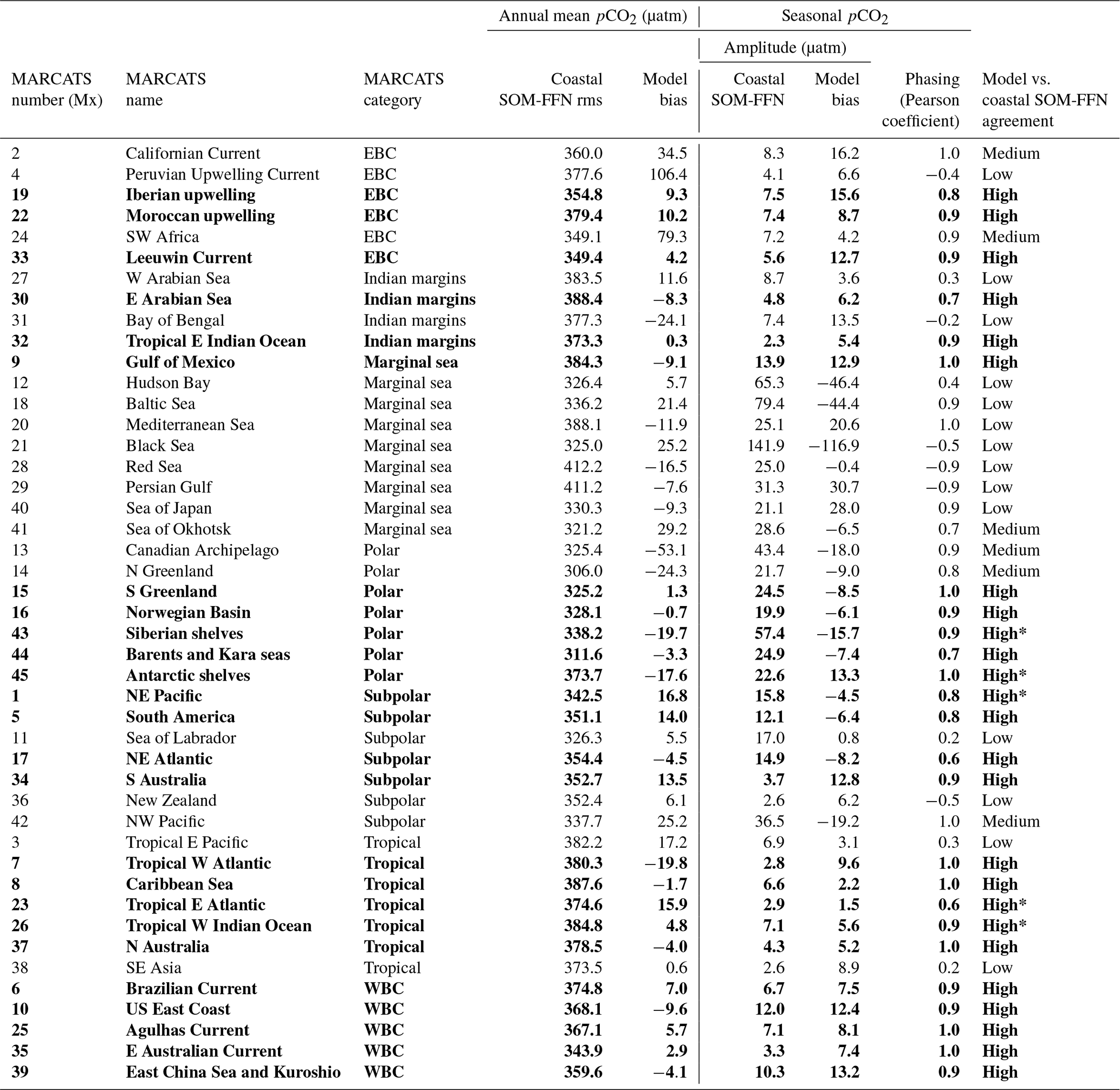
Finally, from this global and regional spatiotemporal evaluation, we label the agreement between the model and coastal SOM-FFN (“high”, “medium” and “low”) for each MARCATS region and identify regions for which our results are the most robust for further in-depth analysis of the processes driving the coastal pCO₂ dynamics. The labels of agreement are based on three criteria. First, we assess whether the simulated annual mean pCO₂ is within 20 µatm of the one extracted from the coastal SOM-FFN. This threshold of 20 µatm roughly corresponds to the globally averaged pCO₂ gradient between the atmosphere and the coastal sea surface (Laruelle et al., 2018). The second and third criteria evaluate the magnitude and phasing of the simulated pCO₂ seasonal cycle against the coastal SOM-FFN using an absolute bias in the seasonal magnitude <20 µatm and a Pearson coefficient > 0.5 as a threshold. The agreement is considered “high” when the three criteria are fulfilled, “medium” when criteria 2 and 3 are satisfied, and “low” when only one (or no) criterion is met for the seasonality.

2.3 Processes controlling seasonal pCO₂ variability: a method tailored for coastal regions

The pCO₂ in surface sea water can be computed from DIC and ALK following Eq. (1) (Sarmiento and Gruber, 2006; Wolf-Gladrow et al., 2007):

$$\begin{array}{}\text{(1)}& {p\mathrm{CO}}_{\mathrm{2}}={\displaystyle \frac{K_{\mathrm{2}}^{\prime }}{K_{\mathrm{0}}^{\prime }{K}_{\mathrm{1}}^{\prime }}}{\displaystyle \frac{(\mathrm{2}\mathrm{DIC}-\mathrm{ALK}{)}^{\mathrm{2}}}{\mathrm{ALK}-\mathrm{DIC}}},\end{array}$$

where $K_{\mathrm{0}}^{\prime }$ is the aqueous-phase solubility constant of CO₂ in water and $K_{\mathrm{1}}^{\prime }$ and $K_{\mathrm{2}}^{\prime }$ represent the apparent equilibrium dissociation constants of the carbonate system. Several physical and biogeochemical processes can thus affect pCO₂ via changes in DIC, ALK and/or via the $\frac{K_{\mathrm{2}}^{\prime }}{K_{\mathrm{0}}^{\prime }{K}_{\mathrm{1}}^{\prime }}$ term, which depends on SST and SSS. To quantify the processes controlling the pCO₂ variability at the seasonal timescale of interest to this study, we adopt the method of Liao et al. (2020). The method starts from the traditional approach that links variations in sea surface ocean pCO₂ to changes in DIC, ALK, SST and SSS using the following linear decomposition (Doney et al., 2009; Lovenduski et al., 2007; Takahashi et al., 1993; Turi et al., 2014):

$$\begin{array}{}\text{(2)}& \begin{array}{rl}\mathrm{\Delta }p{\mathrm{CO}}_{\mathrm{2}}& \approx {\displaystyle \frac{\partial p{\mathrm{CO}}_{\mathrm{2}}}{\partial \mathrm{DIC}}}\mathrm{\Delta }\mathrm{DIC}+{\displaystyle \frac{\partial p{\mathrm{CO}}_{\mathrm{2}}}{\partial \mathrm{ALK}}}\mathrm{\Delta }\mathrm{ALK}\\ & +{\displaystyle \frac{\partial p{\mathrm{CO}}_{\mathrm{2}}}{\partial \mathrm{SST}}}\mathrm{\Delta }\mathrm{SST}+{\displaystyle \frac{\partial p{\mathrm{CO}}_{\mathrm{2}}}{\partial \mathrm{SSS}}}\mathrm{\Delta }\mathrm{SSS},\end{array}\end{array}$$

where Δx terms represent the seasonal anomaly of x (i.e., the departure from the annual mean) and $\frac{\partial p{\mathrm{CO}}_{\mathrm{2}}}{\partial \mathrm{DIC}}$, $\frac{\partial p{\mathrm{CO}}_{\mathrm{2}}}{\partial \mathrm{ALK}}$, $\frac{\partial p{\mathrm{CO}}_{\mathrm{2}}}{\partial \mathrm{SST}}$ and $\frac{\partial p{\mathrm{CO}}_{\mathrm{2}}}{\partial \mathrm{SSS}}$ are coefficients that describe the sensitivity of pCO₂ to changes in DIC, ALK, SST and SSS, respectively. The coefficients for DIC, SST and SSS are always positive as pCO₂ increases with increases in DIC, SST or SSS, while the coefficient for ALK is always negative as pCO₂ systematically decreases with increasing ALK. These coefficients are generally estimated using the approach of Sarmiento and Gruber (2006) (see Eqs. S1–S4 in the Supplement), which has been widely used in the open ocean (Liao et al., 2020; Sarmiento and Gruber, 2006; Takahashi et al., 1993). In this study, we refine the estimation of the coefficients so they can be used for the wide range of DIC $/$ ALK ratios that can be encountered in the coastal waters. This includes conditions when the DIC $/$ ALK ratio is close to 1, such as in regions with significant freshwater discharge like those found near estuarine mouths or on polar shelves subject to sea ice melting when pH is around 7.5 (Egleston et al., 2010). In these cases, the traditional approximation method using mean DIC, ALK, SSS and SST fields breaks down (see Eqs. S1–S2 and Fig. S1 in the Supplement). To circumvent this important limitation, we computed the coefficients of the pCO₂ dependency using a regression approach based on the CO2SYS program (Lewis and Wallace, 1998). At each point in space, pCO₂ was computed using the 1998–2015 average of DIC, ALK, SSS and SST with CO2SYS (method 14 in the CO2SYS MATLAB program, Millero, 2010). The $\frac{\partial p{\mathrm{CO}}_{\mathrm{2}}}{\partial \mathrm{DIC}}$ coefficient was then computed as the slope of the linear regression between pCO₂ and DIC obtained by allowing DIC to vary around the local mean DIC value while keeping other tracers (ALK, SST, SSS) constant. The DIC range used to compute the slope was set to the ± 2 SD of the 1998–2015 monthly values at that location with an upper bound at ± 60 µmol kg⁻¹ (see the Supplement for further details). The same approach was repeated to compute the coefficients for the pCO₂ dependence on ALK, SST and SSS, respectively. Our methodology leads to coefficients that are constant in time but are space dependent. In Fig. S1, we compare the coastal pCO₂ reconstructed from the traditional decomposition (using the space-varying coefficients reported by Sarmiento and Gruber, 2006) with those computed here using the CO2SYS regression. For the global coastal ocean, we find a large bias (global mean root-mean-square error (RMSE) of fitting pCO₂ anomaly in Eq. (2) = 14.6 µatm), which is especially pronounced at high latitudes. In contrast, the decomposition method based on our methodology drastically reduce the biases (global mean RMSE = 2.8 µatm) in coastal regions and allows a more robust reconstruction of the pCO₂ variability.

We further evaluated how using coefficients that vary in both time and space could reduce the residual biases between our pCO₂ decomposition (using space-dependent coefficients that are constant in time) and the pCO₂ simulated in the model that are found in regions with large freshwater discharge, such as the mouth of the Amazon River or Arctic coastal waters. We compare the pCO₂ seasonality simulated by the model to the pCO₂ reconstructed by the following three methods: space-varying coefficients from Sarmiento and Gruber (2006), regression-based space-varying coefficients, and regression-based space- and time-varying coefficients, all of which used a point in the Amazon River plume (1^∘ N, 310.25^∘ E, Fig. S1d and e). At this location, the use of the regression-based coefficients greatly improves the recovery of the simulated pCO₂ compared to using the traditional coefficients of Sarmiento and Gruber (2006), reducing the RMSE from 83 to 24 µatm, corresponding to a bias reduction of 71 %. The use of both space- and time-dependent regression-based coefficients further reduces this bias, bringing down the RMSE from 24 to 18 µatm corresponding to an additional 7 % reduction of the initial bias (83 µatm). Based on these results, we chose to use space dependent only coefficients, which is a simpler approach to implement here and in future studies.

Here we assume that the coefficients are constant in time, and the temporal change in pCO₂ (∂_tpCO₂ in µatm per month) can therefore be expressed as a simple function of the temporal changes in DIC (∂_tDIC), ALK (∂_tALK), SST (∂_tSST) and SSS (∂_tSSS):

$$\begin{array}{}\text{(3)}& \begin{array}{rl}{\partial }_{\mathrm{t}}p{\mathrm{CO}}_{\mathrm{2}}& \approx {\displaystyle \frac{\partial p{\mathrm{CO}}_{\mathrm{2}}}{\partial \mathrm{DIC}}}{\partial }_{\mathrm{t}}\mathrm{DIC}+{\displaystyle \frac{\partial p{\mathrm{CO}}_{\mathrm{2}}}{\partial \mathrm{ALK}}}{\partial }_{\mathrm{t}}\mathrm{ALK}\\ & +{\displaystyle \frac{\partial p{\mathrm{CO}}_{\mathrm{2}}}{\partial \mathrm{SST}}}{\partial }_{\mathrm{t}}\mathrm{SST}+{\displaystyle \frac{\partial p{\mathrm{CO}}_{\mathrm{2}}}{\partial \mathrm{SSS}}}{\partial }_{\mathrm{t}}\mathrm{SSS}.\end{array}\end{array}$$

Temporal changes in DIC, ALK, SST and SSS (∂_tDIC, ∂_tALK, ∂_tSST and ∂_tSSS) are controlled by surface heat flux, ocean transport, freshwater fluxes, biological processes and the air–sea CO₂ flux. Using the model results, we further expand the decomposition to quantify the contribution of these physical and biological processes (see Liao et al, 2020, for details about the derivation):

$$\begin{array}{}\text{(4)}& \begin{array}{rl}& \underset{p{\mathrm{CO}}_{\mathrm{2}}\text{change}}{\underbrace{{\partial }_{\mathrm{t}}p{\mathrm{CO}}_{\mathrm{2}}}}\approx \\ & \underset{\text{circ}}{\underbrace{\left({\displaystyle \frac{\partial p{\mathrm{CO}}_{\mathrm{2}}}{\partial \mathrm{DIC}}}{\partial }_{\mathrm{t}}{\mathrm{DIC}}_{\mathrm{h}}+{\displaystyle \frac{\partial p{\mathrm{CO}}_{\mathrm{2}}}{\partial \mathrm{ALK}}}{\partial }_{\mathrm{t}}{\mathrm{ALK}}_{\mathrm{h}}+{\displaystyle \frac{\partial p{\mathrm{CO}}_{\mathrm{2}}}{{\partial }_{\mathrm{SSS}}}}{\partial }_{\mathrm{t}}{\mathrm{SSS}}_{\mathrm{h}}+{\displaystyle \frac{\partial p{\mathrm{CO}}_{\mathrm{2}}}{\partial \mathrm{DIC}}}{\partial }_{\mathrm{t}}{\mathrm{DIC}}_{\mathrm{v}}+{\displaystyle \frac{\partial p{\mathrm{CO}}_{\mathrm{2}}}{\partial \mathrm{ALK}}}{\partial }_{\mathrm{t}}{\mathrm{ALK}}_{\mathrm{v}}+{\displaystyle \frac{\partial p{\mathrm{CO}}_{\mathrm{2}}}{\partial \mathrm{SSS}}}{\partial }_{\mathrm{t}}{\mathrm{SSS}}_{\mathrm{v}}\right)}}\\ & +\underset{\text{fw}}{\underbrace{\left({\displaystyle \frac{\partial p{\mathrm{CO}}_{\mathrm{2}}}{\partial \mathrm{DIC}}}{\partial }_{\mathrm{t}}{\mathrm{DIC}}_{\text{fw}}+{\displaystyle \frac{\partial p{\mathrm{CO}}_{\mathrm{2}}}{\partial \mathrm{ALK}}}{\partial }_{\mathrm{t}}{\mathrm{ALK}}_{\text{fw}}+{\displaystyle \frac{\partial p{\mathrm{CO}}_{\mathrm{2}}}{\partial \mathrm{SSS}}}{\partial }_{\mathrm{t}}{\mathrm{SSS}}_{\text{fw}}\right)}}\\ & +\underset{\text{bio}}{\underbrace{\left({\displaystyle \frac{\partial p{\mathrm{CO}}_{\mathrm{2}}}{\partial \mathrm{DIC}}}{\partial }_{\mathrm{t}}{\mathrm{DIC}}_{\text{bio}}+{\displaystyle \frac{\partial p{\mathrm{CO}}_{\mathrm{2}}}{\partial \mathrm{ALK}}}{\partial }_{\mathrm{t}}{\mathrm{ALK}}_{\text{bio}}\right)}}\\ & +\underset{\text{thermal}}{\underbrace{\left({\displaystyle \frac{\partial p{\mathrm{CO}}_{\mathrm{2}}}{\partial \text{SST}}}\left({\partial }_{\mathrm{t}}{\mathrm{SST}}_{\mathrm{h}}+{\partial }_{\mathrm{t}}{\mathrm{SST}}_{\mathrm{v}}+{\partial }_{\mathrm{t}}{\mathrm{SST}}_q\right)\right)}}\\ & +\underset{{\mathrm{CO}}_{\mathrm{2}}\text{flux}}{\underbrace{\left({\displaystyle \frac{\partial p{\mathrm{CO}}_{\mathrm{2}}}{\partial \mathrm{DIC}}}{\partial }_{\mathrm{t}}{\mathrm{DIC}}_{{\mathrm{CO}}_{\mathrm{2}}}\text{flux}\right)}},\end{array}\end{array}$$

where the temporal changes in pCO₂ (time tendency called pCO₂ change) are on the left-hand side (LHS) of the equation and the five terms that control this change in pCO₂ are on the right-hand side (RHS) of the equation. Subscripted h and v denote the contribution from horizontal (advection and diffusivity in the meridional and zonal directions) and vertical (vertical advection and diffusivity) transports on SST, SSS, DIC, and ALK; “bio” denotes the DIC and ALK changes induced by biological processes (photosynthesis, respiration, calcium carbonate dissolution and precipitation, denitrification, and nitrification); q denotes the effect of surface heat flux on SST; “fw” denotes the effect of freshwater fluxes (i.e., precipitation, evaporation, river runoff, and sea ice formation and melting) on SSS, DIC, and ALK; and the term CO₂ flux denotes the DIC change induced by air–sea CO₂ exchange.

Here we examine changes in pCO₂ attributed to three oceanic processes that modify the concentration in dissolved species (i.e., DIC, ALK and SSS), namely their transport by oceanic circulation (“circ”, which includes horizontal and vertical transport), the effect of dilution and concentration due to freshwater fluxes (fw), and the effect of biological activity (bio), and these processes isolate the thermal influence tied to SST changes induced by both oceanic transport and air–sea exchange of heat. Finally, the air–sea CO₂ exchange (CO₂ flux) pushes the surface pCO₂ concentration towards its equilibrium with the atmosphere and systematically acts to offset the pCO₂ changes associated with the sum of the internal oceanic processes (circ, bio, fw and thermal). In this study, we apply Eq. (4) using averages between the sea surface and the mixed-layer depth (MLD), defined here as the depth where the water density is 0.01 kg m⁻³ denser than the water at the surface (minimum MLD is 5 m). Positive contributions on the RHS would yield an increase in pCO₂ (positive pCO₂ response on the LHS). Positive values of the CO₂ flux correspond to an ocean CO₂ uptake. This method to decompose the pCO₂ seasonality into controlling processes in the coastal domain is illustrated in three coastal regions: the US East Coast, the US West Coast and the Norwegian Basin.

3 Results and discussion

3.1 Annual mean state and seasonal cycle model evaluation and identification of coastal regions

Figure 1a identifies the coastal regions where the performance of MOM6-COBALT is satisfactory for both the annual mean and the seasonal cycle of pCO₂. The analysis, performed at the MARCATS scale (see Fig. 1b for nomenclature), distinguishes regions of low, medium and high agreement between the model and coastal SOM-FFN, the latter being areas for which our confidence in the identification of the dominant biophysical drivers of the coastal pCO₂ dynamics is highest. This figure will be analyzed in detail in Sect. 3.1.3, but before we do so we first perform a data–model evaluation according to the following procedure. We first evaluate the model by comparing simulated fields of SSS, SST and sea surface nutrients to global and regional observations (Sect. 3.1.1, Figs. 2 and 3). Second, the ability of the model to capture the coastal pCO₂ annual mean and seasonality is assessed against the SOCATv6 data and the continuous monthly observation-based pCO₂ product (coastal SOM-FFN, Laruelle et al., 2017; see Sect. 3.1.2 and Figs. 3–6).

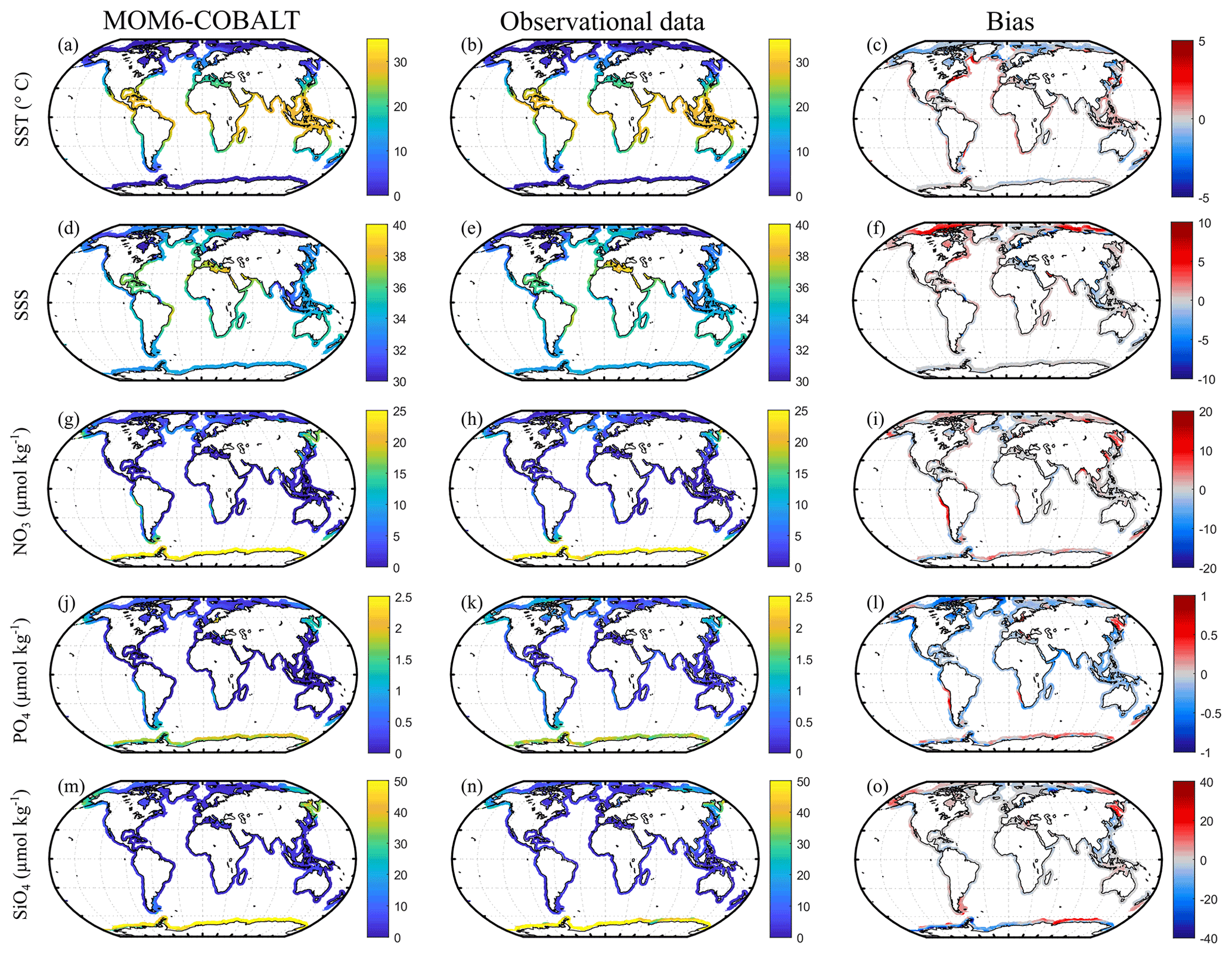
Figure 2 Observed (center) and modeled (left) spatial distributions of the annual mean state of SST (^∘C), SSS (no unit), nitrate (NO₃, µmol kg⁻¹), phosphate (PO₄, µmol kg⁻¹) and silicate (SiO₄, µmol kg⁻¹) and model annual mean bias (right). Observational SST and SSS fields are from the NOAA OI SST V2 (Reynolds et al., 2007) and the EN4 SSS (Good et al., 2013). Observational nutrients are from the World Ocean Atlas version 2018 (Garcia et al., 2019). The bias is the difference between MOM6-COBALT and observed values (red indicates regions where the simulated variables by MOM6-COBALT exceed observed values).

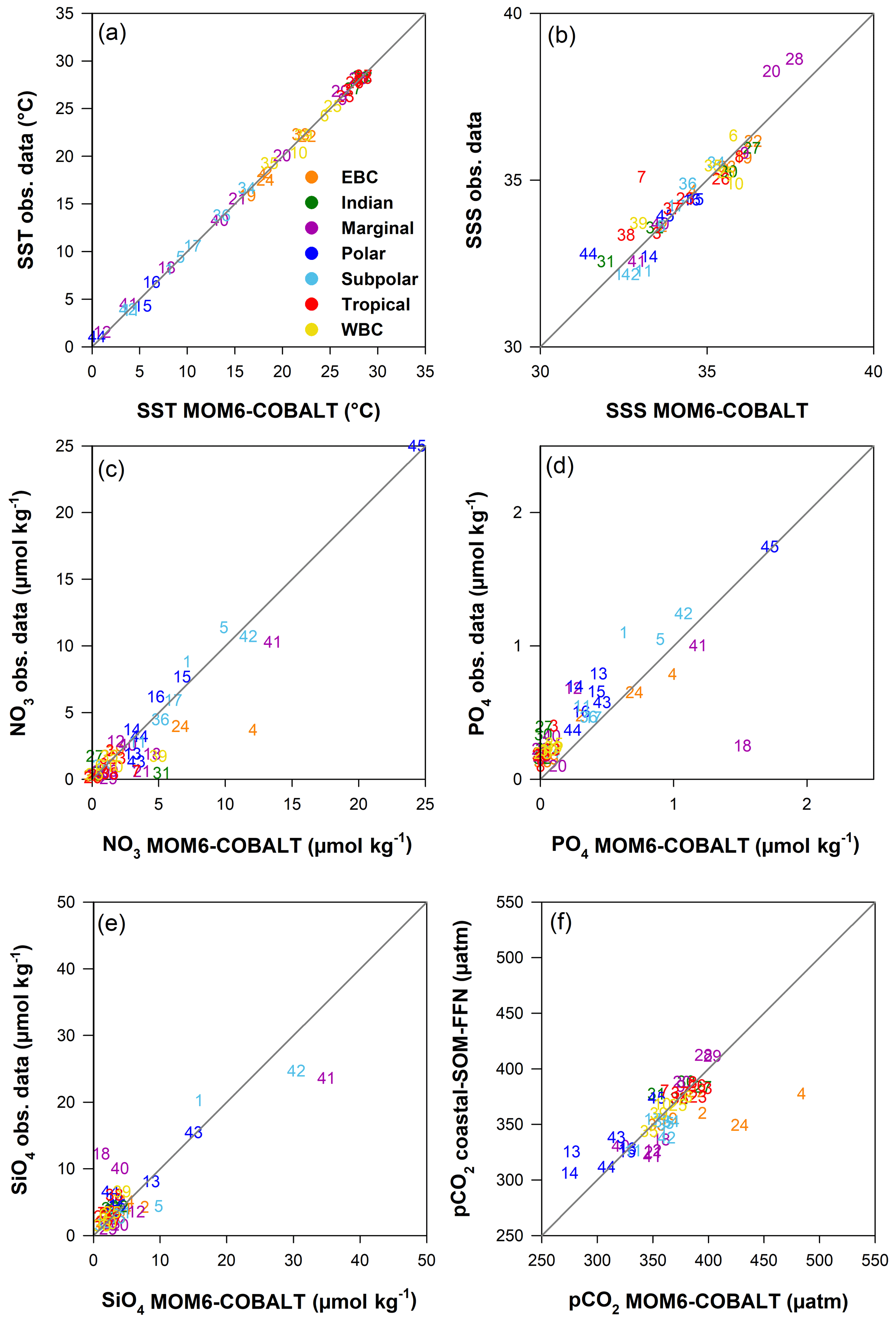
Figure 3 Comparison between observed and simulated annual mean fields in the 45 MARCATS regions: (a) SST (^∘C), (b) SSS (no unit), (c) NO₃ (µmol kg⁻¹), (d) PO₄ (µmol kg⁻¹), (e) SiO₄ (µmol kg⁻¹) and (f) pCO₂ (µatm). Observational datasets are as follows: SST and SSS are from the NOAA OI SST V2 (Reynolds et al., 2007) and the EN4 SSS (Good et al., 2013), nutrients are from the World Ocean Atlas 2018 (Garcia et al., 2019), and pCO₂ is from the coastal SOM-FFN product (Laruelle et al., 2017). Colors correspond to the seven major MARCATS classes (see Fig. 1b). In panels (d) and (e), the Black Sea (M21) is not represented and has xy coordinates of (0.2; 3.5 µmol kg⁻¹) in panel (d) and (10.3; 83.1 µmol kg⁻¹) in panel (e). The Antarctic shelf (M45) is also not represented in panel (e) (55.0;49.1 µmol kg⁻¹).

3.1.1 Model evaluation for coastal waters environmental variables

MOM6-COBALT captures the main spatial patterns of key environmental parameters (SST, SSS and sea surface nutrients) fairly well in the coastal domain (Fig. 2). The global SST field simulated by the model reproduces the strong large-scale tropical to polar SST gradients, with a global median bias of −0.2 ^∘C (Fig. 2a–c), and biases at the scale of MARCATS regions ranging from 0 ^∘C in the NE Atlantic (M17) to 1.3 ^∘C on the US East Coast (M10, Fig. 3a and Table S1). With a global median bias value of 0.2, the model also correctly reproduces the observed SSS patterns that are mainly regulated by evaporation and freshwater inputs from precipitation, riverine runoff and ice melt, with lower SSS values in polar regions and along the coasts of Southeast Asia and higher SSS values along the coasts of evaporation basins such as in the Arabian Sea or the Mediterranean Sea (Fig. 2d–f). The SSS analysis at the MARCATS scale reveals absolute SSS biases that are generally less than or close to 1, except for five MARCATS regions where absolute biases exceed 2. These MARCATS regions are mainly located in marginal seas (the Baltic Sea, M18; the Black Sea, M21; and the Persian Gulf, M29) but also include one polar region (the Canadian Archipelago, M13) and one tropical region (Tropical West Atlantic, M7; see Fig. 3b and Table S1). Similar to SSS, largest the model–data discrepancies for nutrients are mostly found in marginal seas (Fig. 3c–e and Table S1). For instance, the largest PO₄ and SiO₄ biases are encountered in the Black Sea (M21, absolute biases of 3 and 75 µmol kg⁻¹, respectively). The Peruvian Upwelling Current (M4), the Bay of Bengal (M31) and the NE Pacific (M1) also present large biases in NO₃ and PO₄ (e.g., NO₃ bias of 8 µmol kg⁻¹ for M4). However, the global median nutrients biases are much smaller, reaching 0.3, −0.2 and −0.4 µmol kg⁻¹ for nitrate (NO₃, Fig. 2i), phosphate (PO₄, Fig. 2l) and silicate (SiO₄, Fig. 2o), respectively.

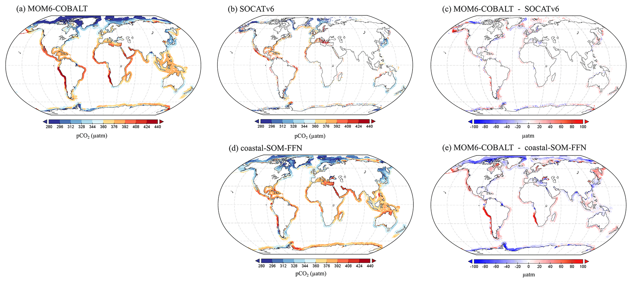
Figure 4 Spatial distributions of the annual mean pCO₂ (µatm) generated by (a) MOM6-COBALT and (b) extracted from the SOCATv6 database, (c) model bias given as the difference between panels (a) and (b) (in µatm; red and blue colors correspond to regions in which the pCO₂ simulated by MOM6-COBALT is higher and lower than SOCATv6, respectively). (d) Spatial distribution of the annual mean pCO₂ from the coastal SOM-FFN product (Laruelle et al., 2017). (e) Model bias given as the difference between panels (a) and (d).

The model–data seasonal evaluation reveals that MOM6-COBALT reproduces the global SST and SSS amplitudes remarkably well (median absolute bias of 0.1 ^∘C and 0.0, respectively; see Table S2 in the Supplement). Some exceptions can nevertheless be diagnosed, such as in the marginal Black Sea (M21), where the bias in SST seasonal amplitude reaches −1.3 ^∘C, and in three MARCATS regions (Bay of Bengal, M31; tropical West Atlantic, M7; and Siberian shelves, M43) where the SSS seasonal biases are larger than 0.4. The model–data comparison also reveals that the phasing of the SST and SSS seasonal cycles are in very good agreement (Pearson correlation close to 1) for all 45 MARCATS regions, with the exception of four for which significant deviations in SSS are found, i.e., two marginal seas (Hudson Bay, M12, and the Red Sea, M28) and along the Californian Current (M2) and Brazilian Current (M6). The nutrients analysis shows absolute global median biases in seasonal amplitude of 0.1, 0.0 and 0.7 µmol kg⁻¹ for NO₃, PO₄ and SiO₄, respectively. Seven MARCATS regions present absolute biases larger than 1.5 µmol kg⁻¹ that are mainly located in marginal seas (Baltic Sea, M18; Sea of Japan M40; and Sea of Okhotsk, M41) but also in polar (Siberian, M43, and Antarctic, M45, shelves) and subpolar (NE Pacific, M1) regions and in the Bay of Bengal (M31). The model–data comparison sometimes shows significant phase shifts in their seasonal signal (Pearson coefficient < 0.5), such as for MARCATS regions located in Indian and tropical margins, marginal seas, and EBCs.

3.1.2 Model evaluation for coastal pCO₂

The spatial distribution of the annual mean pCO₂ simulated by MOM6-COBALT is in good agreement with the observational pCO₂ values extracted from the SOCATv6 database with generally low pCO₂ values (blue colors) in temperate and high latitudes and high pCO₂ values (yellow and red colors) in tropical and sub-tropical regions (Fig. 4a–c). The model–data pCO₂ evaluation at the regional scale shows that 33 of the 45 MARCATS present absolute biases lower than 20 µatm (Table S1). The regions where the bias exceeds this threshold include two EBCs (the Californian Current, M2, and the Peruvian Upwelling Current, M4), two marginal seas (Sea of Japan, M40, and Sea of Okhotsk, M41), and one polar region (Antarctic shelves, M45), a subpolar region (NW Pacific, M42) and the tropical East Atlantic (M23) shelf. Note that in some MARCATS regions, in particular in marginal seas and Indian seas, there are no SOCATv6 observations to perform the comparison (e.g., the Bay of Bengal, M31; see Fig. 4b and Table S1). Hence, we also evaluate the performance of MOM6-COBALT against the continuous coastal SOM-FFN pCO₂ product, which uses a neural network interpolation method to fill data gaps and resolve the spatiotemporal coastal pCO₂ variability globally.

Our results show that MOM6-COBALT reproduces the main spatial features of the annual mean pCO₂ field captured by the coastal SOM-FFN product, as revealed by the relatively low globally averaged bias of 2.5 µatm (Fig. 4a and d). In both the model and the SOM-FFN product, low coastal pCO₂ values are consistently found in temperate and high-latitude regions in both hemispheres, while high pCO₂ values are largely limited to (sub-)tropical regions. The largest discrepancies (Fig. 4e) are found at high latitudes (poleward of 60^∘ N and 60^∘ S, negative bias), along the Peruvian and Namibian upwelling systems (high positive bias) and more locally close to the mouth of some large rivers (e.g., the plume of the Amazon or the Rio de la Plata, high negative bias). We note, however, that these regions are poorly sampled in the SOCATv6 dataset (Fig. 4b) and are thus likely weakly constrained in the coastal SOM-FFN product (Fig. 4d).

At the regional scale, differences in annual mean pCO₂ between MOM6-COBALT and coastal SOM-FFN are lower than 20 µatm in 35 MARCATS (Table S1, Fig. 3f), which partly is a reflection of the low annual mean biases observed in the environmental driver variables in these regions (see Sect. 3.1.1). In EBC, WBC and subpolar coastal regions, the model tends to overestimate the regional mean pCO₂ compared to coastal SOM-FFN (positive bias), except along the US East Coast (M10), in the East China Sea and Kuroshio (M39), and in the NE Atlantic (M17, Table S1). In polar regions, the model generally underestimates the mean pCO₂ compared to coastal SOM-FFN, except around S Greenland (M15). In Indian, marginal, and tropical coastal regions, no general trend can be identified regarding the sign of the bias, which can be positive or negative.

Quantitatively, the 10 MARCATS regions with absolute biases > 20 µatm are mainly located in regions for which very limited or no observational data have been compiled in the SOCATv6 database (Table S1) and/or for which large discrepancies can already be identified at the level of the master environmental variables (Sect. 3.1.1). These regions mainly belong to EBCs (three out of the six EBC MARCATS regions) and marginal seas (three out of the nine marginal seas MARCATS regions), with the remaining four being either polar (the Canadian Archipelago, M13, and the N Greenland, M14), subpolar (NW Pacific, M42) or Indian margins (the Bay of Bengal, M31). The largest biases are found in the Peruvian Upwelling Current (M4), SW Africa (M24), the Californian Upwelling Current (M2) and the Canadian Archipelago (M13), with biases of 106, 79, 35 and −53 µatm, respectively.

Our analysis reveals that the seasonal amplitudes simulated by MOM6-COBALT are systematically larger than the ones estimated by the coastal SOM-FFN product (Fig. 5a–b, red colors in Fig. 5c and positive biases in Table S2) for all coastal regions belonging to EBC, WBC, and Indian and tropical margins. For the majority of the polar and subpolar margins and for some marginal seas, the model simulates lower seasonal pCO₂ amplitudes (blue colors in Fig. 5c and negative biases in Table S2). Quantitatively, absolute biases between the modeled and coastal SOM-FFN amplitudes do not exceed 20 µatm, except for in marginal seas where larger discrepancies are calculated (six of the nine marginal MARCATS regions, Table S2). The monthly mean pCO₂ seasonal cycle simulated by MOM6-COBALT is also well in phase (Pearson correlation coefficients > 0.5) with the one extracted from coastal SOM-FFN in 34 out of the 45 MARCATS regions (Fig. 5d and Table S2). The agreement is especially good in the best-monitored MARCATS regions (MARCATS where > 50 % of the area is covered by SOCATv6 observations, Table S1). For instance, in regions with good data coverage, such as along the US East Coast (M10), the Norwegian Basin (M16), the Californian Current (M2), the Leeuwin Current (M33) or the Brazilian Current (M6), the Pearson correlation coefficient is higher than 0.9 (Table S2). In contrast, the seasonal pCO₂ cycle simulated by MOM6-COBALT substantially diverges from that of the coastal SOM-FFN in four poorly monitored marginal seas and in a few of regions of EBCs, Indian margins, subpolar margins, and tropical margins (Pearson correlation coefficient < 0.5, Table S2 and Fig. 5d).

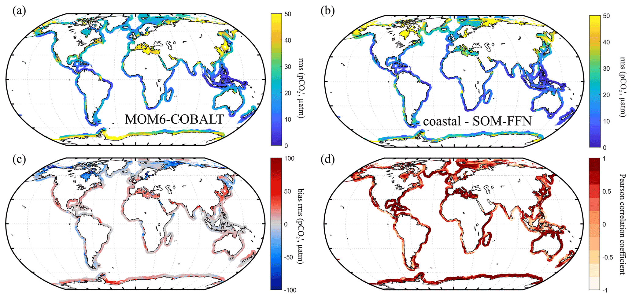
Figure 5 Seasonal variability in ocean pCO₂ (µatm). Seasonal amplitude (a) simulated by MOM6-COBALT model and (b) in the coastal SOM-FFN product, and (c) bias between the model and coastal SOM-FFN seasonal amplitude (red indicates that simulated amplitude exceeds coastal SOM-FFN). The seasonal amplitude is expressed as the root mean square of the monthly climatology pCO₂ anomalies (${\mathrm{rms}}_{p{\mathrm{CO}}_{\mathrm{2}}^{\prime }}$, µatm). (d) Pearson correlation coefficient of the regression between the seasonal pCO₂ cycles calculated by MOM6-COBALT and coastal SOM-FFN. A value of 1 indicates that both signals are perfectly in phase with one another, while a value of −1 represents a complete phase shift.

The model pCO₂ seasonal evaluation against SOCATv6 is only performed in 11 MARCATS regions, namely the Californian Current (M2), tropical E Pacific (M3), the Gulf of Mexico (M9), the US East Coast (M10), S Greenland (M15), Norwegian Basin (M16), NE Atlantic (M17), Iberian upwelling (M19), Moroccan upwelling (M22), China Sea and Kuroshio (M39), and New Zealand (M36). The modeled seasonal cycle is in good agreement with the one derived from SOCATv6 (Fig. 6b–l, Table S2) with absolute biases < 20 µatm for all of the 11 selected MARCATS and Pearson correlation coefficients close to 0.5 or higher except for the Iberian Upwelling (M19, Pearson value of 0.2) and on the New Zealand shelf (M36, value of 0.3). We did not perform the SOCATv6 model seasonal evaluation for the other MARCATS regions because the vast majority of grid cells only include data for less than 4 climatological months (Fig. 6a). However, we also evaluated the simulated pCO₂ seasonality against SOCATv6 in regions where this evaluation is not possible to be performed at the MARCATS scale. To do so, we selected four sites of smaller spatial extent than MARCATS for which we calculated climatological seasonal pCO₂ signals from the SOCATv6 dataset and compared them with the model pCO₂. These sites are located off the Antarctic Peninsula, on the Queensland Plateau in NE Australia, in coastal waters of Papua New Guinea and off Terra Nova in Antarctica (see black boxes in Fig. 6a). In those regions, the absolute biases of the seasonal amplitude between MOM6-COBALT and SOCATv6 (Fig. 6m–p) are less than 20 µatm, and the phase in the seasonal cycles presents a good agreement with a Pearson correlation coefficient value of 0.8, except for the Papua New Guinea data (value of 0.5). Note that the model SOCATv6 seasonal evaluation for Terra Nova presents a good agreement, but the MARCATS scale (Sea of Labrador, M11) evaluation to which this region belongs to reveals a low agreement, showing that a poor agreement between coastal SOM-FFN and the model does not equate to poor model skill when these regions are undersampled by SOCATv6.

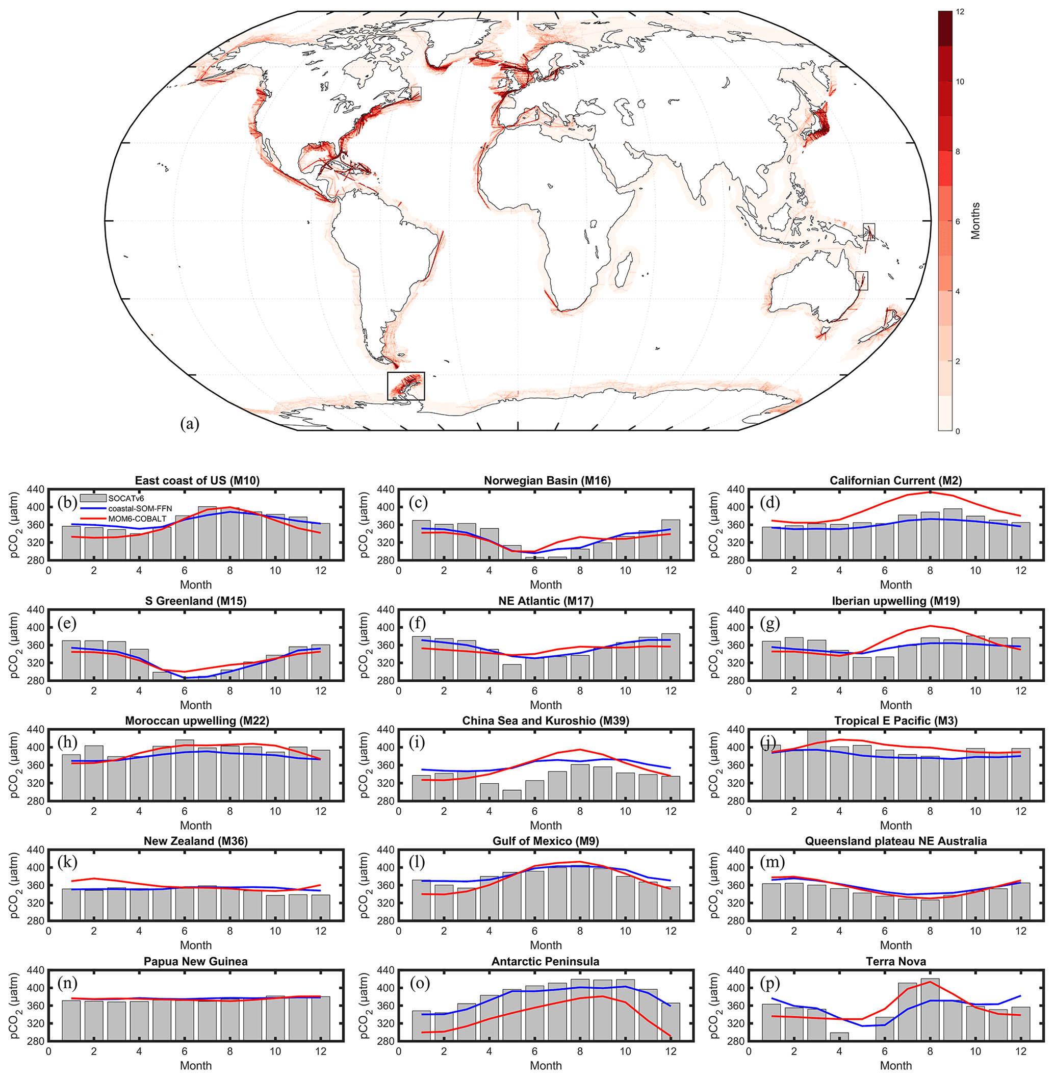
Figure 6 (a) SOCATv6 temporal coverage evaluated as the number of months (1 to 12) where at least one pCO₂ measurement is available (see details in Sect. 2). Seasonal pCO₂ cycle (µatm) derived from SOCATv6 (bar in gray) and coastal SOM-FFN (in blue) and simulated by MOM6-COBALT (in red) for several MARCATS regions (b–l) and four coastal sites of smaller spatial extent than a MARCATS region (m–p). The location of the four coastal sites is represented by black boxes in panel (a). Month 1 corresponds to January. For consistency in the y axis between panels, the value of 276 µatm is not represented in panel (p) for month 5 for the SOCATv6 data.

3.1.3 Identifying coastal regions of high model to coastal SOM-FFN agreement

Overall, the pCO₂ spatiotemporal analysis model–data evaluation shows that out of 45 MARCATS regions, 29 have an absolute bias for their annual mean < 20 µatm when MOM6-COBALT-coastal SOM-FFN, MOM6-COBALT-SOCATv6 and coastal SOM-FFN-SOCATv6 are compared (Table S1). Together, these 29 MARCATS regions represent 65 % of the global coastal ocean surface area. For the 11 MARCATS regions that are best covered by observations (MARCATS regions where > 50 % of the surface area is covered by SOCATv6 observations, Table S1), absolute biases for the annual mean are always < 20 µatm for the three product intercomparison, except in the Californian Current (M2), in the Baltic Sea (M18) and along the NE Pacific (M1). The seasonal MOM6-COBALT against coastal SOM-FFN evaluation also reveals that 39 of the 45 MARCATS regions have pCO₂ seasonal amplitude biases < 20 µatm and that 34 MARCATS regions have a Pearson correlation coefficient > 0.5 (Table S2).

Based on this evaluation, we attribute for each MARCATS region a level of confidence in the model to coastal SOM-FFN agreement (“high”, “medium” and “low”; see Table 1 and Fig. 1a). Out of the 45 MARCATS regions, 25 are labeled with high agreement, meaning that they fulfill the following criteria regarding the annual mean and the seasonality (Table 1 and dotted MARCATS regions in Fig. 1a): a bias < 20 µatm in the annual mean pCO₂ between MOM6-COBALT and coastal SOM-FFN, a bias < 20 µatm in the magnitude of the seasonal pCO₂ cycle, and a seasonal phase characterized by a Pearson correlation coefficient > 0.5. Note that the some MARCATS regions, i.e., the Siberian shelf (M43), the Antarctic shelf (M45), the NE Pacific (M1), the tropical E Atlantic (M23) and the tropical W Indian Ocean(M26), also present an annual mean pCO₂ bias < 20 µatm in the MOM6-COBALT-SOCATv6 and coastal SOM-FFN-SOCATv6 comparisons (Table S1). In addition, seven high-agreement MARCATS regions also show a data density > 50 % (this comes to 13 MARCATS regions if we lower the data coverage to > 30 %, Fig. 1a). These 7 MARCATS regions are located in contrasted coastal environments, i.e., three EBCs (Iberian upwelling, M19; Moroccan upwelling, M22; and the Leeuwin Current, M33), one WBC (US East Coast, M10), one Polar region (Norwegian Basin, M16), one subpolar region (NE Atlantic, M17) and one marginal sea (Gulf of Mexico, M9). These seven high-agreement MARCATS regions could also result from the very good correspondence between the data–model annual mean and seasonal patterns in environmental fields (Table S1 and Table S2, except M22, M33 and M9 for the nutrient phasing) and are therefore excellent potential candidates for an analysis of the processes controlling the coastal pCO₂ dynamics. A total of six additional MARCATS regions fulfill the criteria related to the seasonal pCO₂ evaluation, but they fail to fulfill the annual mean pCO₂ bias threshold of 20 µatm. These medium-agreement regions (Table 1 and dashed regions in Fig. 1a) include two EBCs (Californian Current, M2, and SW Africa, M24), one marginal sea (Sea of Okhotsk, M41), two polar regions (Canadian Archipelago, M13, and N Greenland, M14) and one subpolar region (NW Pacific, M42) shelves. The majority of marginal seas are systematically associated with large biases relating to either pCO₂ or the main environmental variables. These regions fulfill only one criterion (or none of them) regarding the pCO₂ seasonality, and they are hence labeled as low-agreement regions (Table 1, Fig. 1a). Other low-agreement regions include one EBC (Peruvian Upwelling Current, M4), one Indian region (Bay of Bengal, M31), two tropical regions (tropical E Pacific, M3, and SE Asia, M38), two subpolar regions (Sea of Labrador, M11, and New Zealand, M36) and one WBC region (Brazilian Current, M6).

3.1.4 Methodological limitations

While our results show a relatively good agreement between MOM6-COBALT and coastal SOM-FFN regarding the spatial and temporal pCO₂ distribution over the global coastal ocean, the comparison remains challenging for several reasons.

First, while the climatology of Laruelle et al. (2017, coastal SOM-FFN) is currently the best available product for a model–data comparison, it has its own limitations. For instance, in some regions, particularly for coastal upwellings such as the Moroccan (M22) and Peruvian (M4) upwellings, the pCO₂ fields generated by the coastal SOM-FFN do not reproduce the high and variable pCO₂ values measured in situ well (see, e.g., Friederich et al., 2008; McGregor et al., 2007). Such poor performance of the coastal SOM-FFN algorithm in these types of systems has already been identified by Laruelle et al. (2017). Indeed, upwelling regions are still relatively poorly monitored and expand partly beyond the coastal domain used by Laruelle et al. (2017), leading to locally skewed calibration of the SOM-FFN. Deficiencies in the observation-based product can thus partly explain the large model–data bias (106 µatm, the largest of all MARCATS regions) calculated in the Peruvian upwelling region. Moreover, although the Surface Ocean CO₂ Atlas database (SOCAT) has expanded significantly over the past few years, some regions are still poorly monitored. In the coastal regions where no observational data exist (e.g., in the Black Sea, the Sea of Okhotsk, the Bay of Bengal, Fig. 4b) in the SOCAT database used here (SOCATv6, Bakker et al., 2016), it is difficult to evaluate the performance of the SOM-FFN and thus of an Oceanic General Circulation Model (OGCM) in reproducing the pCO₂ field. In addition, for certain regions subjected to complex dynamic biogeochemical settings (e.g., upwelling, seasonal cover of sea ice, influenced by rivers, marginal seas), the pCO₂ field reconstructed by the SOM-FFN suffers from poor performance, which can partly be explained by the lack of observational data. This lack of observations could partly explain why MOM6-COBALT-coastal SOM-FFN pCO₂ biases exceed 20 µatm in these regions. The seasonal model evaluation against SOCATv6 is limited at the MARCATS scale and mainly performed against coastal SOM-FFN due to the very few coastal regions that contain a continuous climatological seasonal pCO₂ cycle (Fig. 6a) in the SOCATv6 database. This study highlights the regions (Fig. 1a, e.g., Indian ocean margins, the Peruvian upwelling, marginal seas) where new observational data are most urgently needed, specifically those collected during periods of the year that are currently not covered, to improve our understanding of the CO₂ exchange between coastal regions and the atmosphere at the regional and global scales. In addition, only one global continuous pCO₂ climatology derived by the SOM-FFN method currently exists for the coastal ocean. It would therefore be beneficial for the community to develop other observation-based climatologies relying on other interpolation techniques, as is currently the case for the open ocean.

Second, the model–data comparison should also be analyzed in the light of the current limitations in the model itself. OGCMs have been designed for global ocean applications, and the coarse spatial resolution of these models, on the order of 0.5^∘ in the present study, cannot accurately resolve mesoscale and sub-mesoscale processes and tidal mixing in shelf regions even with a model configuration including parameterizations for these processes. The coastal currents are also not always well resolved because of the coarse resolution of the shelf bathymetry. These small-scale hydrodynamic features are known to affect the spatiotemporal variability of pCO₂ and the air–sea CO₂ exchange (Bourgeois et al., 2016; Kelley et al., 1971; Lachkar et al., 2007; Laruelle et al., 2010). Therefore, although MOM6-COBALT runs at 0.5^∘, discrepancies between coastal SOM-FFN and MOM6-COBALT in narrow EBCs such as the Peruvian Upwelling Current (M4) and along SW Africa (M33) could also be explained by the limited spatial resolution of the model. Moreover, OGCMs such as MOM6-COBALT have a relatively simple representation of biogeochemistry that does not fully capture some of the important processes of the carbon dynamics in coastal waters, such as sea ice temporal dynamics (Adcroft et al., 2019), neritic calcification (O'Mara and Dunne, 2019), or terrestrial and marine organic matter decomposition and burial (Lacroix et al., 2021a, b). Moreover, the largest biases observed in marginal seas can partly be explained by large fluvial inputs and oceanic water flows through fine-scale topography (e.g., straits) that are poorly represented in global OGCMs.

Finally, the annual mean and seasonal pCO₂ biases between the coastal SOM-FFN and MOM6-COBALT can also be traced back to divergences in the environmental fields simulated by the model compared to observations (Tables S1 and S2). For instance, in most marginal seas, the model poorly resolves the annual mean and seasonal cycle of SSS and nutrients compared to the observations. These discrepancies impact the simulated pCO₂ via the controls of the SSS on the CO₂ solubility and of nutrients on the biological pump and CO₂ uptake. In the tropical W Atlantic (M7), which is under the influence of the Amazon River, the model simulates lower annual mean SSS (and therefore lower pCO₂) than the observations. In the tropical E Pacific (M3) and in Southeast Asia (M38), the poor agreement between simulated and observed seasonal pCO₂ cycle could be explained by significant biases in the nutrient seasonal cycles (low Pearson correlation coefficient). Interestingly, some regions reveal significant biases in the major environmental fields but not in the pCO₂ (e.g., the tropical W Atlantic, M7), while in other regions the reverse is observed (e.g., the Mediterranean Sea, M20; W Arabian Sea, M27; and in New Zealand, M36). In addition, for some regions biases in environmental fields do not affect the pCO₂ as expected. For instance, along the US East Coast (M10), MOM6-COBALT simulates larger SST compared to observations, while the simulated pCO₂ is lower compared to coastal SOM-FFN on an annual mean. This clearly shows that biases in environmental fields are not sufficient to fully explain the biases in pCO₂ diagnosed between MOM6-COBALT and coastal SOM-FFN.

3.2 Processes governing the seasonal pCO₂ variability

Our second objective is to examine the drivers of the pCO₂ seasonality in three well-sampled and contrasted coastal regions where the model to coastal SOM-FFN agreement is satisfactory: the US East Coast (M10), the Norwegian Basin (M16) and the Californian Current (M2). The US East Coast is a sink of atmospheric CO₂ that has been extensively studied over the past decade (e.g., Fennel et al., 2019; Laruelle et al., 2015; Shadwick et al., 2010, 2011; Signorini et al., 2013). The pCO₂ spatiotemporal dynamics in this MARCATS region are particularly well captured by MOM6-COBALT (high agreement, Fig. 1a), despite an annual mean SST bias of 1.3 ^∘C in the data–model comparison in this region (Table S1). Because the SST amplitude and seasonal phasing are in agreement between the model and data (Table S2), the bias in the mean SST does not impact the seasonal pCO₂ cycle (Pearson correlation coefficient > 0.5 and bias < 20 µatm in the seasonal pCO₂ amplitude, Table 1). We also selected the Californian Current because it is a source of CO₂ to the atmosphere and because, similar to the US East Coast, it ranks among one of the best-monitored coastal regions in the world (e.g., Evans et al., 2011; Fennel et al., 2019; Hales et al., 2012; Turi et al., 2014). In this region, the model is classified as medium agreement (Table 1 and Fig. 1a). Indeed, the simulated seasonal cycle of pCO₂ is in relatively good agreement with coastal SOM-FFN (Figs. 5–6, and Table 1) despite biases in the annual mean pCO₂ compared to observations (Fig. 3f) and a phase shift in the seasonality of SSS and nutrients (Pearson correlation coefficient < 0.5). However, the Californian Current is also one of the few coastal regions where an analysis of the processes controlling the pCO₂ seasonality has already been performed using a regional biogeochemical model and sequential simulation removing processes one after the other (Turi et al., 2014), which can hence be compared to our analysis. Finally, the choice of the Norwegian Basin is motivated by the good performance (high agreement) of the model and the intense atmospheric CO₂ sink that occurs in this contrasted region.

3.2.1 Seasonality along the US East Coast

The seasonal evolution of pCO₂ averaged over the US East Coast (M10) is represented in Fig. 7a. Ocean pCO₂ is at a minimum in winter (February–March ∼ 331 µatm), increases through spring and peaks in summer (August, ∼ 400 µatm) before decreasing again in autumn. Figure 7b reveals the complex interplay of the four ocean internal processes (thermal and biological processes, ocean circulation, and freshwater flux) on the seasonal pCO₂ variability that can either act in synergy or oppose each other.

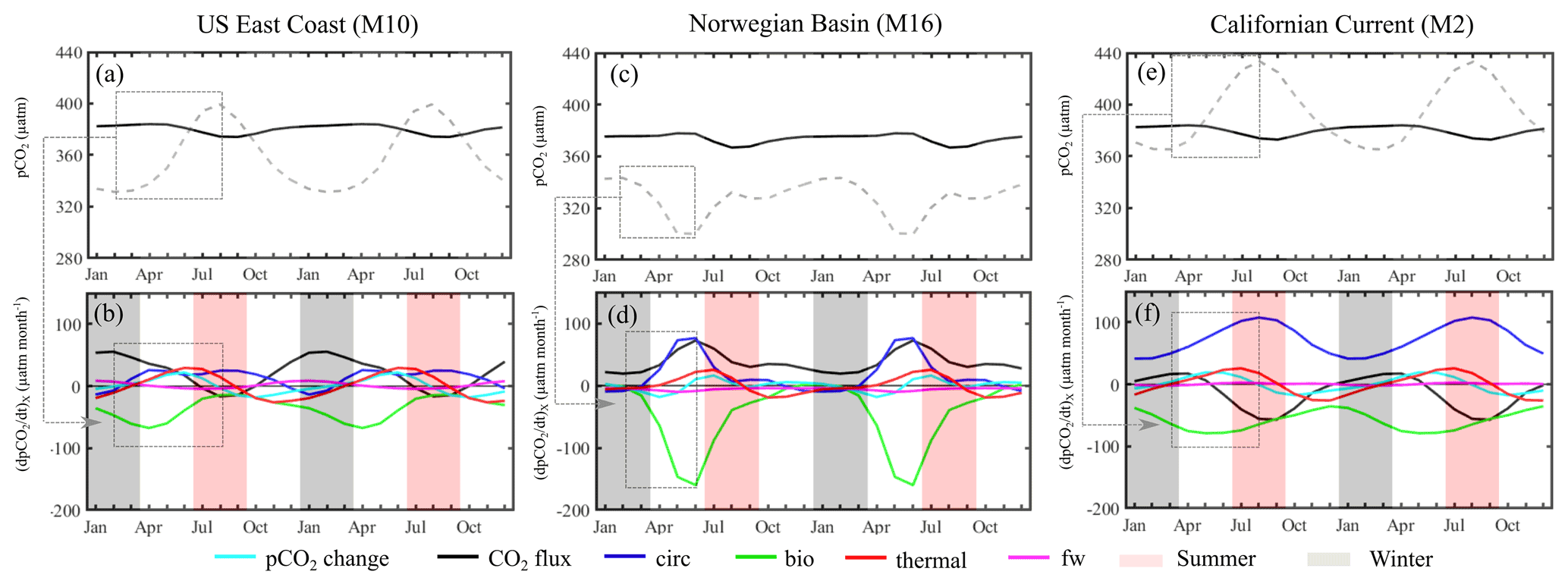
Figure 7 Processes controlling the ocean pCO₂ seasonal cycle. Mean seasonal sea surface pCO₂ (dashed line) and atmospheric pCO₂ (black line; in µatm) simulated by MOM6-COBALT and detrended over (a) the US East Coast (M10), (c) the Norwegian sea (M16) and (e) the Californian current (M2). Spatially averaged contributions (in µatm month⁻¹) from biological activity (bio, green), temperature changes (thermal, red), transport of chemical species (circ, blue), freshwater flux (fw, pink) and the CO₂ air–sea flux (CO₂ flux, black) controlling the pCO₂ temporal change (pCO₂ change, cyan) for the three regions (b, d, f). A positive value corresponds to an increase in sea surface pCO₂. Winter corresponds to the months of January, February and March, and summer corresponds to the months of July, August and September.

The thermal effect (thermal, red line in Fig. 7b) increases pCO₂ from early spring to summer by decreasing the solubility of CO₂. In contrast, the solubility of CO₂ increases in autumn and winter, inducing a decline in pCO₂. The largest changes in pCO₂ associated with the change in SST occur during spring (29 µatm per month in June) and autumn (−26 µatm per month in November). This thermal effect was already identified by Signorini et al. (2013) in their observational study and further confirmed by Cai et al. (2020). These authors highlighted that lowest pCO₂ was generally reported in winter or at the beginning of spring and highest pCO₂ in summer or autumn, despite significant temporal and spatial heterogeneity between the different sub-regions of the US East Coast (Scotian shelf, the Gulf of Maine, the Georges Bank and Nantucket shoals, the Middle Atlantic Bight, and the South Atlantic Bight). The effect of biological processes above the mixed-layer depth (bio, green line) reduces pCO₂ throughout the year, revealing that primary production exceeds organic matter degradation in the surface layer all year long. The largest pCO₂ decrease associated with biological processes is observed in early spring (values of −68 µatm per month in April), which is well documented (e.g., Shadwick et al., 2010, 2011; Signorini et al., 2013). The transport of chemical species by ocean circulation (circ, blue line) increases pCO₂ and tends to oppose biological processes year-round except at the end of autumn and beginning of winter. This pCO₂ increase induced by the circulation term is at its maximum in April (26 µatm per month). Throughout the year, the contribution of freshwater fluxes (fw, pink line) remains minor compared to the other terms (maximum absolute value of 9 µatm per month in January). For each month and season, the air–sea CO₂ exchange term (CO₂ flux, black line) counteracts change in pCO₂ associated with ocean internal processes taking place in surface seawater (sum of bio, circ, thermal and fw). The CO₂ flux term increases pCO₂ at the sea surface (acting as an atmospheric CO₂ sink) throughout the year, except during summer (between July and September) where it decreases sea surface pCO₂ and releases CO₂ towards the atmosphere (acting as an atmospheric CO₂ source). This year-round simulated atmospheric CO₂ uptake (except for the summer season) is also in agreement with previous literature (Fennel et al., 2019; Laruelle et al., 2015; Signorini et al., 2013). The study of Laruelle et al. (2015) has nevertheless shown that in spring the southern part of the US East Coast is quasi-neutral and that in autumn some regions, such as the Gulf of Maine or the Georges Bank, act as a CO₂ source. The temporal change of pCO₂ (pCO₂ change, cyan line) is the result of the non-perfect balance between the internal processes and the air–sea CO₂ flux.

We evaluate the rate of change tied to each process during the marked peak-to-peak pCO₂ increase observed between winter and summer (from 331 µatm in February to 400 µatm in August, Fig. 7a). A positive rate of change (in µatm per month) indicates that the process contributes to an increase in pCO₂ between winter and summer (February–August). This process-based analysis reveals that the winter-to-summer pCO₂ increase on the US East Coast (M10) mainly results from thermal (rate of change $=+\mathrm{5}$ µatm per month) and ocean circulation (rate of change $=+$4 µatm per month) influences combined with a large reduction of the biological CO₂ uptake (rate change of +7 µatm per month, Fig. 7b). The importance of the thermal and circulation effects and the presence of a strong biological drawdown are in line with results from past studies (e.g., Laruelle et al., 2015; Shadwick et al., 2010, 2011; Signorini et al., 2013; and Cai et al., 2020). Our results identify the reduction of biological carbon uptake as a key control of pCO₂ seasonality and thus agree with the studies of Shadwick et al. (2010, 2011) but slightly diverge compared to those of Signorini et al. (2013) or Laruelle et al. (2015), which found that the thermal effect was the dominant driver. This difference is largely explained by the different levels of details in the decomposition method. While most model studies, including ours, use seasonal change in SST, SSS, DIC and ALK, observational approaches cannot isolate the compounding changes tied to biological activity from those of ocean transport.

3.2.2 Seasonality in the Norwegian basin and in the Californian Current

The pCO₂ seasonal cycle in the Norwegian Basin (M16) and the Californian Current (M2) simulated by MOM6-COBALT are represented in Fig. 7c and e, respectively. The Norwegian Basin shows a near-constant pCO₂ value (∼330 µatm) throughout the year, except in spring when it drops by 30 µatm (minimum pCO₂ value of 300 µatm in June). The phasing of the seasonal pCO₂ cycle in the Californian Current is similar to that along the US East Coast, with a minimum pCO₂ value of 366 µatm in March followed by an increase that reaches a maximum pCO₂ value of 433 µatm in August and then decreases again at the beginning of autumn.

The decomposition of the seasonal cycle into different processes for both the Norwegian Basin and the Californian Current (Fig. 7d and f) reveal patterns that are qualitatively similar to those already diagnosed for the US East Coast (Fig. 7b). For both shelf regions, the biological and circulation effects remain negative and positive, respectively, throughout the year, while the thermal effect increases pCO₂ in spring and summer but decreases pCO₂ in autumn and winter. The freshwater term is also minor compared to the other terms. Quantitatively, however, the amplitude of the different terms points to different first-order control in the pCO₂ seasonality for each region. The amplitudes are calculated here using the marked peak-to-peak change in pCO₂, which occurs between February and June in the Norwegian basin and between March and August in the Californian Current.

In the Norwegian basin, the strong winter to summer pCO₂ decreases (43 µatm, Fig. 7c) are mainly associated with the large and rapid CO₂ uptake associated with the spring phytoplankton bloom (biological rate of change $=-\mathrm{45}$ µatm per month on average between February and June, with a maximum pCO₂ uptake of −175 µatm per month in June, Fig. 7d). This biological drawdown is only partly compensated for by the supply of high pCO₂ water masses from the ocean circulation (rate of change $=+$24 µatm per month). These dynamics are consistent with the fact that the Norwegian Basin is one of the most productive regions of the world and is characterized by a well-documented, intense spring bloom (e.g., Findlay et al., 2008). In addition, the effect of thermal changes only plays a comparatively minor role here (rate of change $=+$7 µatm per month).

In contrast to the US East Coast and the Norwegian Basin, the analysis performed in the Californian Current reveals that circulation is the main driver of the winter-to-summer pCO₂ increases (68 µatm, Fig. 7e). The upwelling of high-pCO₂ waters increases year-round surface pCO₂. However, its influence is weaker in winter than in summer, thereby explaining the pCO₂ increase observed between February and August (rate of change $=+$12 µatm per month, Fig. 7f). This large contribution from circulation is consistent with the simulations of Turi et al. (2014), who identified the ocean transport associated with upwelling in the Californian Current as the dominant process, and the higher intensity of the summer upwelling and its impact on pCO₂ were also reported in prior work (e.g., Evans et al., 2015; Fiechter et al., 2014; Turi et al., 2014). In this region, biological processes also oppose the effect of ocean circulation, with upwelled deep water bringing nutrients to the surface and stimulating phytoplankton productivity (e.g., Evans et al., 2015; Fiechter et al., 2014; Turi et al., 2014). However, it plays a minor role in the pCO₂ increase (rate of change ∼ 0 µatm per month) and the thermal effect (rate of change $=+\mathrm{4}$ µatm per month).

4 Conclusions

In this study, an OGCM (MOM6-COBALT) that is primarily designed for the open ocean was used to examine sea surface pCO₂ seasonality in the coastal domain. We first evaluated the ability of the model to reproduce the spatial and temporal dynamics of key environmental variables, such as SST, SSS and sea surface nutrients, against in situ observations. The spatiotemporal variability of coastal pCO₂ was also evaluated using direct coastal pCO₂ observations from the SOCAT database (SOCATv6, Bakker et al., 2016) and a global observational continuous monthly pCO₂ climatology available at high spatial resolution (coastal SOM-FFN, Laruelle et al., 2017).

Our model–data comparison showed a relatively good agreement on the environmental variables spatiotemporal distribution except for some coastal regions mainly located in marginal seas. Our results also revealed a relatively good agreement, both in time and space, between pCO₂ from MOM6-COBALT, coastal SOM-FFN and SOCATv6, and most of the discrepancies between the three products are found in regions with poor data coverage, such as in the Bay of Bengal, the Sea of Okhotsk or Hudson Bay (Fig. 1a). This study highlights the regions (Fig. 1a, e.g., Indian Ocean margins, Peruvian upwelling, marginal seas) where new observational data are most urgently needed, specifically data collected during different periods of the year that are currently missing to improve our understanding of the CO₂ exchange between coastal regions and the atmosphere at the regional and global scales. From the model–data evaluation, we identified regions where the MOM6-COBALT model shows the highest agreement in reproducing the spatial and seasonal pCO₂ variability, and where the different processes governing the pCO₂ dynamics can be examined with reasonable confidence (high- and medium-agreement regions in Table 1 and Fig. 1a).

We also adapted a novel method to quantify the contributions of the different physical and biological processes governing the sea surface pCO₂ seasonality in the coastal domain. This method goes one step further than past coastal studies (e.g., Signorini et al., 2013; Turi et al., 2014) where the processes attribution was only based on the seasonal changes in DIC, ALK, SST and SSS and/or combined with a series of sequential simulations isolating one term after the other. In particular, our simulations are non-sequential and allow us to account for the co-variations between the different variables impacted by each process and how their simultaneous evolution modulates pCO₂ dynamics in quantitative terms. Our approach, which is illustrated in three coastal regions (the US East Coast, the California Current and the Norwegian Basin), allows to decipher the complex interplay between ocean transport of chemical species (DIC, ALK and SSS), biological drawdown, freshwater fluxes (dilution and concentration effects) and thermal changes (air–sea fluxes and transport of temperature) on the pCO₂ dynamics. Depending on the season and region, these terms can reinforce or oppose each other and act to strengthen or dampen the amplitude of pCO₂ seasonal variations that control the air–sea CO₂ exchange. Along the US East Coast and in the Californian Current, pCO₂ increases from winter to summer. In the former region, this increase is controlled by a subtle balance between biological drawdown, thermal changes and ocean circulation, while in the Californian Current the circulation due to the upwelling (supplying pCO₂-rich waters to the surface) drives the increase in pCO₂. In contrast, in the Norwegian Basin biological drawdown dominates the marked spring pCO₂ decrease observed in the region. These differences in the quantitative controls of pCO₂ dynamics from one region to another support our proposed analysis at the broad scale of the 45 MARCATS regions that together compose the global coastal ocean.

A handful of observation-based studies have analyzed the seasonal variability of pCO₂ in the global coastal ocean (Cao et al., 2020; Chen and Hu, 2019; Laruelle et al., 2017). The mechanistic understanding of seasonal pCO₂ variations was and remains limited by the amount of available observations. The modeling approach tailored for the coastal ocean presented in this paper complements observational studies and helps to improve our quantitative understanding of the underlying physical and biological drivers of coastal pCO₂ dynamics. The comparison of the model performance to a state-of-the-art coastal pCO₂ database and continuous pCO₂ data product also lends confidence to our model results for a large fraction of the global coastal domain. The coastal ocean is under tremendous anthropogenic pressure (e.g., climate, land-use change, agriculture, pollution, urbanization; see, e.g., Mackenzie et al., 2005; Regnier et al., 2013; Seitzinger et al., 2005). Understanding the interplay between physical, biological and thermal processes and how they control coastal pCO₂ worldwide will be key to assessing how their future changes impact air–sea CO₂ exchange in coastal environments.