the Creative Commons Attribution 4.0 License.
the Creative Commons Attribution 4.0 License.
 | 05 May 2022
Contribution of a constellation of two wide-swath altimetry missions to global ocean analysis and forecasting
Mounir Benkiran
Pierre-Yves Le Traon
Gérald Dibarboure
Swath altimetry is likely to revolutionize our ability to monitor and forecast ocean dynamics. To meet the requirements of the EU Copernicus Marine Service, a constellation of two wide-swath altimeters is envisioned for the long-term (post-2030) evolution of the Copernicus Sentinel 3 topography mission. A series of observing system simulation experiments (OSSEs) is carried out to quantify the expected performances. The OSSEs use a state-of-the-art high-resolution (∘) global ocean data assimilation system similar to the one used operationally by the Copernicus Marine Service. Flying a constellation of two wide-swath altimeters will provide a major improvement of our capabilities to monitor and forecast the oceans. Compared to the present situation with three nadir altimeters flying simultaneously, the sea surface height (SSH) analysis and 7 d forecast error are globally reduced by about 50 % in the OSSEs. With two wide-swath altimeters, the quality of SSH 7 d forecasts is equivalent to the quality of SSH analysis errors from three nadir altimeters. Our understanding of ocean currents is also greatly improved (30 % improvements at the surface and 50 % at 300 m depth). The resolution capabilities will be drastically improved and will be closer to 100 km wavelength compared to about 250 km today. Flying a constellation of two wide-swath altimeters thus looks to be a very promising solution for the long-term evolution of the Sentinel 3 constellation and the Copernicus Marine Service.
- Article
(39803 KB) - Full-text XML
- BibTeX
- EndNote


The Copernicus Marine Service is one of the six pillar services of the European Union Copernicus programme (Le Traon et al., 2019). It provides regular and systematic reference information on the physical and biogeochemical ocean and sea-ice state for the global ocean and the European regional seas. After 7 years of operation, the Copernicus Marine Service is recognized internationally as one of the most advanced service capabilities in ocean monitoring and forecasting and has involved more than 30 000 expert services and users worldwide (Le Traon et al., 2021).
The Copernicus Marine Service is highly dependent on the timely availability of comprehensive satellite and in situ observations (Le Traon et al., 2019). Satellite altimetry plays a prominent role thanks to global, real time, all-weather sea level measurements, which provide a strong constraint for inferring 4D ocean circulation through data assimilation (see a review in Le Traon et al., 2017). Copernicus Marine Service modelling and data assimilation systems depend substantially on the status of the altimeter constellation (e.g. Hamon et al., 2019). Four altimeters at least are required. The main limitation of classical altimetry is the 1D nature of altimeter measurements, which provide sea level measurements only at the sub-satellite point (i.e. nadir point), thus creating large unobserved gaps in the cross-track direction (Chelton et al., 2001). These authors also point out that the distance between altimetry satellite tracks and the revisit time decrease with the inverse of the number of satellites, so there is a strong diminishing return associated with classical altimetry. As a result, only wavelengths longer than 200 km are well represented.
Wide-swath altimetry that will be demonstrated with the Surface Water Ocean Topography (SWOT) mission (Morrow et al., 2019) addresses these limitations. Through a series of observing system simulation experiments (OSSEs), Benkiran et al. (2021) and Tchonang et al. (2021) demonstrated that SWOT data could be readily assimilated in a global high-resolution (∘) analysis and forecasting system with a positive impact everywhere and very good performances. The main limitation of SWOT is, however, related to its long-term repeat period. In the longer run, flying a constellation of two wide-swath altimeters would thus be highly beneficial to further improve performance, in particular for smaller spaces and shorter timescales.
The impact of a constellation of two wide-swath altimetry missions has been analysed as part of two studies carried out by Mercator Ocean International (MOi) for the European Space Agency (ESA). This was done in close collaboration with the French Space Agency (CNES), which led a 2.5-year (2018–2020) phase A study called WiSA (Wide-Swath Altimetry). WiSA aimed to define an innovative concept of an altimetry system to provide new measurements for both oceanography and hydrology on an operational basis (CNES, 2020). The targeted programmatic framework is the Sentinel-3 topography mission (post-2030), the follow-up to Sentinel-3, which will address the expected evolution of the Copernicus Space Component. The first ESA study carried out by Bonaduce et al. (2018) in the north-east Atlantic regional model showed that a constellation of three nadir and two wide-swath altimeters could reduce ocean analysis errors by up to 50 % compared to three nadir altimeters operating alone. The second ESA study (this paper) extends this work to the global ocean using the wide-swath altimeter system characteristics analysed as part of the WiSA phase A. The study also uses the latest version of the Copernicus Marine Service global ∘ modelling and data assimilation system and the OSSE design used for SWOT OSSEs presented in Benkiran et al. (2021) and Tchonang et al. (2021).
Results for this global study are presented and discussed in this paper, which is organized as follows. The WiSA concept is presented in Sect. 2. Section 3 details the OSSE methodology. Results are discussed in Sect. 4, and Sect. 5 provides the main conclusions and recommendations of the study.
The WiSA concept was developed in a Phase A study carried out by CNES and the industry as a tentative follow-up to the SWOT mission. The goal of the WiSA concept was to leverage the main improvement of SWOT's swath altimeter (i.e. 2D images of sea surface topography and near-nadir radar backscatter, lower noise floor than nadir altimeters for the same ground pixel surface) with significant changes to better address the needs of operational oceanography and hydrology, while making the satellite simpler, smaller and more affordable than the SWOT precursor mission.
Arguably the main weakness of SWOT is temporal sampling: with a single satellite and a 120 km swath, it is simply impossible to resolve the timescales of the small-scale features that will be observed by SWOT. At least two (three) wide-swath altimeters are needed to ensure that 68 % (80 %) of 50 km features in the global ocean can be observed with a mean revisit time of 5 d or less. Moreover, Lamy and Albouys (2014) explain how the SWOT orbit was a trade-off between multiple constraints for this research mission: technical constraints from the instrument, optimization for the aliasing of tides, sampling optimized for a single satellite. In contrast, the so-called WiSA Phase A orbit was selected by CNES using the methodology of Dibarboure et al. (2018) to maximize the sampling for one- to three-swath altimeter satellites (or swath–nadir hybrid constellations). This Sun-synchronous orbit has an altitude of approximately 750 km ( revolutions per day), and the altimeter swath covers latitudes up to 82∘. With an exact repeat of 17 d (i.e. good enough for tidal aliasing despite being Sun-synchronous), the orbit also has so-called sub-cycles of 2 and 5 d, both of which maximize the distribution of observations in space and time for wind or wave applications and small to medium mesoscale applications. Moreover, the optimal space–time sampling for two satellites is achieved when the first and second swath altimeters are on the same orbit plane, separated by a 180∘ angle on the orbit circle. This property, discussed by CNES (2020), is important for technical and practical considerations (e.g. ground station visibility, compatibility with other sensors with a wider swath).
The second difference between SWOT and WiSA is their respective noise levels. SWOT tries to achieve an unprecedented spectral noise floor of 2 cm2 cycles per kilometre (i.e. of the order of 1.36 cm RMS (root mean squared) for 2 km × 2 km pixels) in order to resolve wavelengths as small as 15 km (i.e. a feature diameter of 8.5 km). Because the goal of WiSA is to resolve wavelengths of only 50 km, CNES and Thales Alenias Space selected a simpler technical design (i.e. cheaper and more robust) for the interferometer baseline. The resulting noise is of the order of 2.7 cm RMS for 2 km × 2 km products. Note that because the high-frequency noise is random, it can be averaged out in pixels of varying size. In other words, it is possible to select different resolution-versus-precision trade-offs from the same spectral noise floor (e.g. sub-centimetric precision for a 5 km product or 5 cm precision for a 1 km product). More importantly, while larger than SWOT, the noise floor of the WiSA concept is more than sufficient to ensure that all scales up to 50 km are well observed, even in relatively high wave conditions (wave height modulates the noise floor of all altimeters according to a linear relationship). Using the methodology of Vergara et al. (2019) and spectral slopes and wave climatologies obtained from Jason altimeters, CNES (2020) reports that WiSA has a mean observability (i.e. wavelength where the signal to noise ratio is 1) of 37 km or better, over more than 80 % of the global ocean.
The other components of the WiSA error budget (e.g. wet troposphere, roll) combine the requirement of SWOT (Esteban-Fernandez, 2013) for the small scales and the accuracy of nadir altimeters for the large scales. In essence, the WiSA concept ensures that the end-to-end error budget is less than 10 % of the SLA along-track power spectral density up to 1000 km, with a RMS less than 2.5 cm, including large-scale errors (e.g. precise orbit determination biases, ionosphere residual). In practice, the SWOT simulator (Gaultier, 2016) is a good approximation of the error budget for OSSE studies. The simulator also captures the complex 2D nature of correlated error sources of WiSA which are similar to SWOT.
3.1 Ocean model
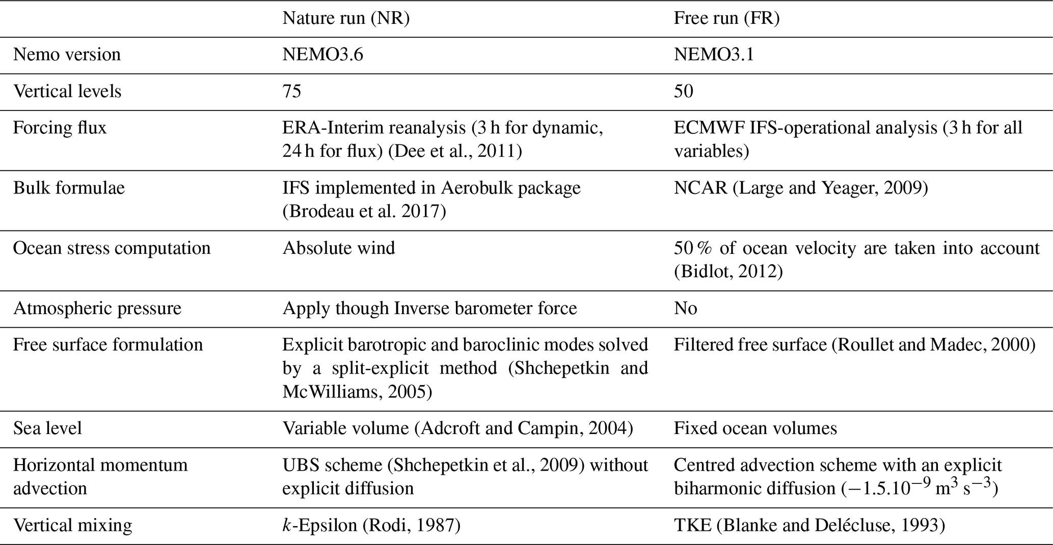
The MOi global ocean forecasting system (see Lellouche et al., 2018, 2013), which delivers forecast products for the Copernicus Marine Service, is used in this study. As described in the literature (Errico et al., 2013), OSSEs use two different models or model configurations. In our study, we use the same NEMO ∘ resolution model (Nucleus for European Modelling of the Ocean, Madec and The Nemo Team, 2008) but with different configurations and forcings. The first uses a free NEMO3.6 simulation (Nature Run hereafter referred to as NR) to represent the real ocean and simulate all the synthetic observations for the study. The second model is used to assimilate synthetic observations from the NR. This model uses the NEMO3.1 model with a different and less energetic configuration. Table 1 lists all these differences. A detailed description and validation of the NR is presented in Benkiran et al. (2021).
Table 1Differences in model parameterization between the nature run (NR) and assimilated model (AR) (Benkiran et al., 2021).
3.2 Simulation of observations and noise
All simulated observations were extracted from the NR simulation and these observations were collected over a period of 15 months (from 1 October 2014 to 31 December 2015), which includes the period covered by the OSSEs. Sea surface height (SSH) data were simulated along three nadirs and two wide-swath altimeters (S1 and S2).
The three nadir altimeters correspond to Jason-3 (or Sentinel-6 already is in the same orbit) (J3) and the nadirs of each of the two wide-swath altimeters S1 and S2. The along-track nadir altimeter data were extracted from NR at the 1 Hz frequency corresponding to a spatial resolution of 6–7 km from hourly mean fields of the NR. A random noise of 3 cm was added to along-track data to take into account altimeter measurement noise (i.e. close to the 1 Hz error budget of the nadir altimeter of the SWOT satellite). For the two swath altimeters, the WiSA Phase A orbit (S1) selected by CNES (Dibarboure et al., 2018) was used together with a second (S2) on the same orbit plane, separated by a 180∘ angle on the orbit circle. All SSH data were simulated from the NR using the Jet Propulsion Laboratory's (JPL) SWOT Simulator (Gaultier et al., 2016). The simulator constructs a regular grid based on the baseline orbit parameters of the satellite. The simulator models the most significant errors that are expected to affect the data, i.e. the KaRIn (Ka-band Radar Interferometer) noise, roll errors, phase errors, baseline dilation errors, wet troposphere and timing errors. In this study, we only used the estimated WiSA KaRIn noise derived for a significant wave height (SWH) of 2 m. Figure 1 shows the standard deviation of the KaRIn random error considering across-swath resolutions of 1 km (solid line) and 6 km (dashed line) as a function of the cross-track distance in kilometres.
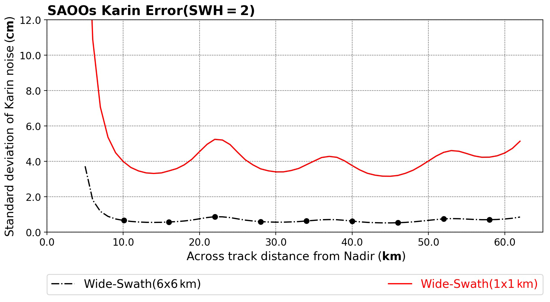
Figure 1The curves displayed show the wide-swath instrumental error with SWH = 2 m (wave height), considering across-swath horizontal resolution of 1 km (solid red line) and 6 km (dashed black line).
Figure 2a shows the SSH from the NR at a given central date of our 7 d assimilation cycle (analysis window) over the Kuroshio region. Data coverage along the tracks of the three nadir altimeters over the 7 d analysis window is shown in Fig. 2b while Fig. 2c shows the coverage of the combination of two wide-swath altimeters. It can be observed that with two wide-swath altimeters the ocean is almost covered by the measurements over a 7 d time period.
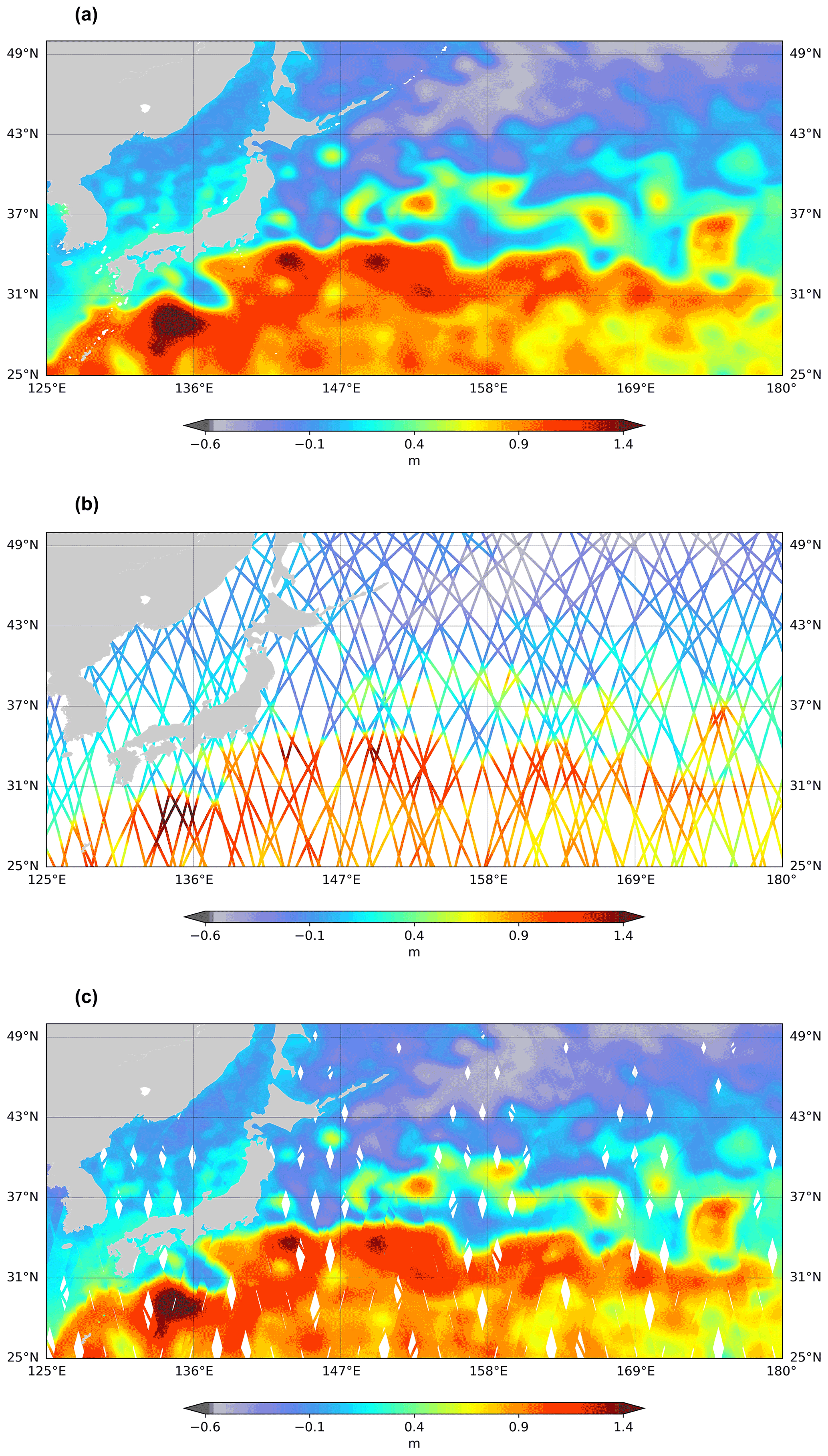
Figure 2(a) SSH from the truth run (NR) on 4 January 2015; (b) simulated along-track data from Jason3, nadirs of S1 and S2 for 7 d assimilation cycle; and (c) simulated S1+S2 data (1–8 January 2015).
To make OSSEs close to the MOi global analysis and forecasting system, other assimilated data were simulated: satellite sea surface temperature, in situ temperature and salinity data (Argo), and the ice concentration data (see details in Benkiran et al., 2021).
3.3 Data assimilation
An updated version of the data assimilation scheme developed at MOi, called SAM2 (Système d'Assimilation Mercator V2) and described by Lellouche et al. (2018), was used. SAM is a reduced-order local Kalman filter for which the analysis subspace is constructed using a band-passed times series of model states from free simulation. Several improvements and adaptations of this system were made for this study. In particular, a four-dimensional (4D) version of the assimilation scheme is used, in which the analysis uses a 4D subspace and produces daily models correction of SSH, temperature, salinity and velocity field. All these updates and their impacts on the system performance are described in Benkiran et al. (2021).
3.4 Experimental set-up
Starting from the satellite altimetry simulated data obtained from the NR run, three global OSSEs were carried out using a different NEMO configuration but the same spatial resolution of ∘ (∼7 km). OSSE0 is the Free Run (FR) of the ocean model used to assess the performance of the other experiments. OSSE1 corresponds to nadir (3N) altimetry data assimilation. Finally, OSSE2 (3N + 2S) assimilated all observation types (combining two swaths and three nadirs). OSSE1 and 2 also assimilate sea surface temperature (SST), ice concentration (IC), and temperature and salinity (T/S) profile data.
Our simulations start from a free model state on 1 October 2014. A 3-month simulation (until the end of December 2014) was carried out with assimilation of SSH along the nadirs (3N) together with SST, IC and T/S data. This allows us to avoid the spin-up period in our experiments. All the experiments shown here start from the same state on 1 January 2015.
Results of the impact of assimilation of the SSH from the three nadir altimeters and from the two wide-swath altimeters combined with the three nadir altimeters are detailed in this section. These results are obtained by comparing each experiment with our real ocean (NR) data over a period of 10 months (1 March to 30 December 2015). Results are presented below: impact on SSH analyses and forecasts; impact on the different time and space scales; spectral and coherence analyses in a series of selected rectangular areas (boxes); and impact on velocity, temperature and salinity.
4.1 Impact on sea-level analyses and forecasts
The SSH variance in the NR computed over one year (2015) is shown in Fig. 3. The SSH variance shows high variability in the more energetic regions such as the Gulf Stream (GS), Kuroshio (KS), Antarctic Circumpolar Current (ACC), Brazil–Malvinas confluence (BM) and Agulhas (AG). The SSH variance in the NR compares very favourably with real altimeter observations (as detailed in Benkiran et al., 2021).

Figure 3SSH variance (in cm2) in the NR over the period from February to December 2015. The boxes denote the rectangular sub-regions for which wavenumber spectra and coherence analyses were performed.
The temporal evolution of SSH error variance over the global ocean for each experiment is compared in Fig. 4. This variance decreases over a few weeks (6 weeks) to reach a stable state for the analyses (continuous lines) and the forecasts (dotted lines). The assimilation of the swath altimeter data reduces analysis errors from 15.6 cm2 (black line) to 10.1 cm2 (red line), a reduction of 54 %. The gain is of about 46 % for the forecasts (dotted lines). These are major improvements. In particular, with two swath altimeters, 7 d SSH forecasts are as good as SSH analyses derived from three nadir altimeters.
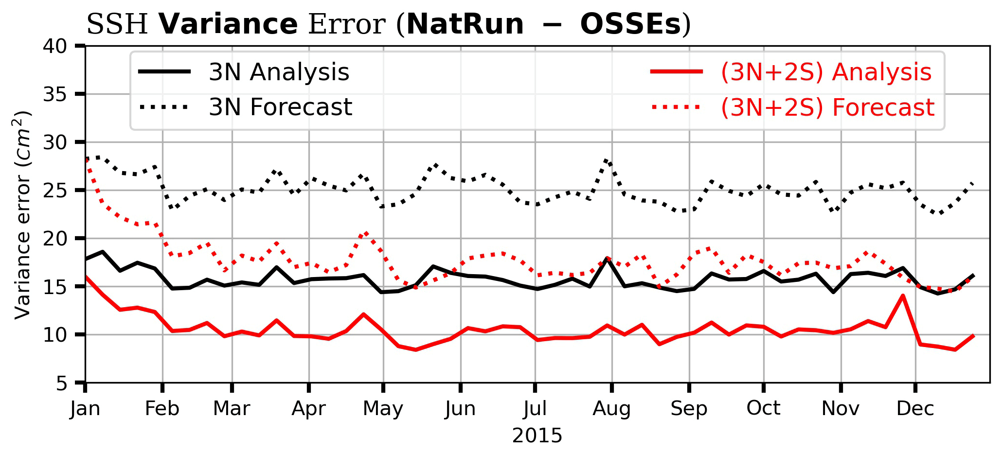
Figure 4The temporal evolution of the SSH error variance in global ocean analysis and forecast over 2015. Results obtained by comparing the SSH ocean analysis (solid lines) and forecast (dash lines) with the SSH from the NR. Experiments with assimilation of three nadirs (3N) (black lines) and with assimilation of three nadirs and 2 swath altimeters (3N + 2S) (red lines).
To analyse the results further, the relative variance VAR∗ (in terms of percentage), which represents the error variance (VarError) relative to the FR error variance. The expression of this relative variance is as follows:
Here we use the error variance (difference between NatRun and OSSEs) as follows:
is the temporal variance of SSH error obtained by comparing the NR with a given OSSE at a given location x and y over a period of t 363 d with i=1; 2 refers to the ith OSSE and T refers to the maximum time.
VarError represents the variance error for each experiment (OSSEi). This variance of the error is calculated by comparing each OSSE with the NR.
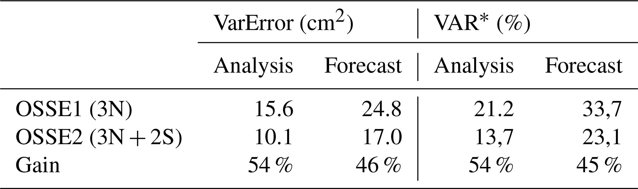
Global maps of SSH analysis error variance (VarError) for these experiments are presented in Fig. 5. The Free Run (FR) has a fairly large variance (Fig. 5a) especially over western boundary currents: Antarctic Circumpolar Current (ACC), Indian Ocean (IND), Brazil–Malvinas confluence (BM) and Agulhas current (AG). The assimilation of SSH data from the three nadir altimeters (3N) in addition to the SST data and salinity and temperature profiles significantly reduced this error (Fig. 5b) over the global ocean. The assimilation of SSH from the swath altimeter in addition (Fig. 5c) greatly reduced this error over the global ocean. A fairly significant improvement can be observed in specific areas (boxes in Fig. 5b) such as the Gulf Stream, the Antarctic Circumpolar Current and the Kuroshio Current. Figure 6, which represents the difference in error between the 3N assimilation and the 3N + 2S assimilation, shows the contribution of the assimilation of the combination of the wide-swath altimeters and the nadir altimeters compared to the nadir altimeters. This improvement (error reduction) is visible on almost 80 % of the ocean points. The results of the impact of the wide-swath altimeter data on SSH in the global ocean are summarized in Table 2. Adding the swath altimeters improves the analyses and forecasts by about 50 % (54 % for analysis, 45 % for forecast). With the assimilation of wide-swath altimeters, the error relative to the FR error variance (VAR∗ – columns 3 and 4 in Table 2) is only 13.7 % and 23.1 % for analyses and forecasts respectively.
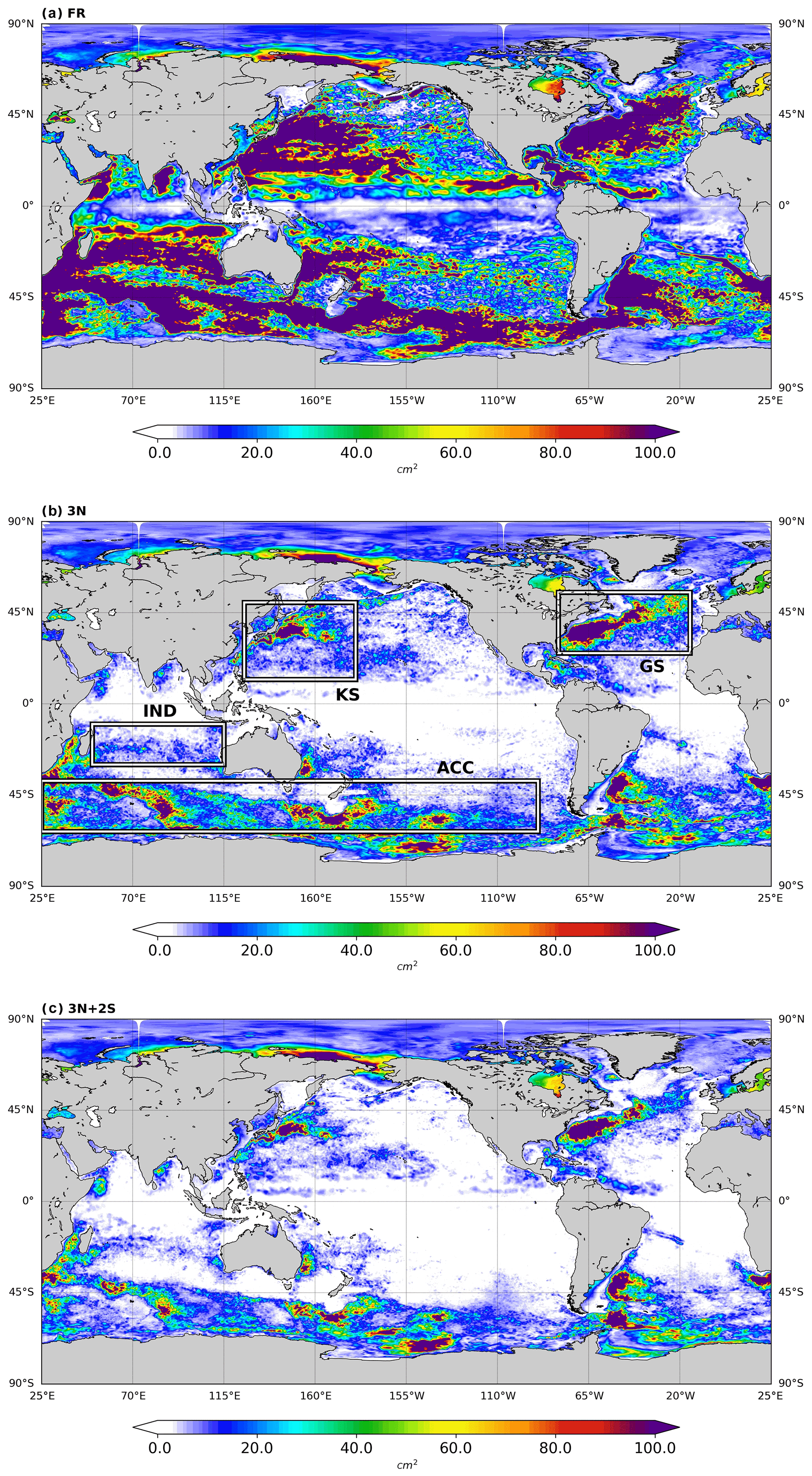
Figure 5Global maps of SSH analysis error (NR – model analysis) variance (in cm2, 2015). (a) Free run (FR); (b) with three nadirs (3N); (c) assimilation of three nadir and two wide-swath instruments (3N + 2S). In panel (b), GS: Gulf Stream, ACC: the Antarctic Circumpolar Current, KS: Kuroshio Current and IND: South Indian Ocean.
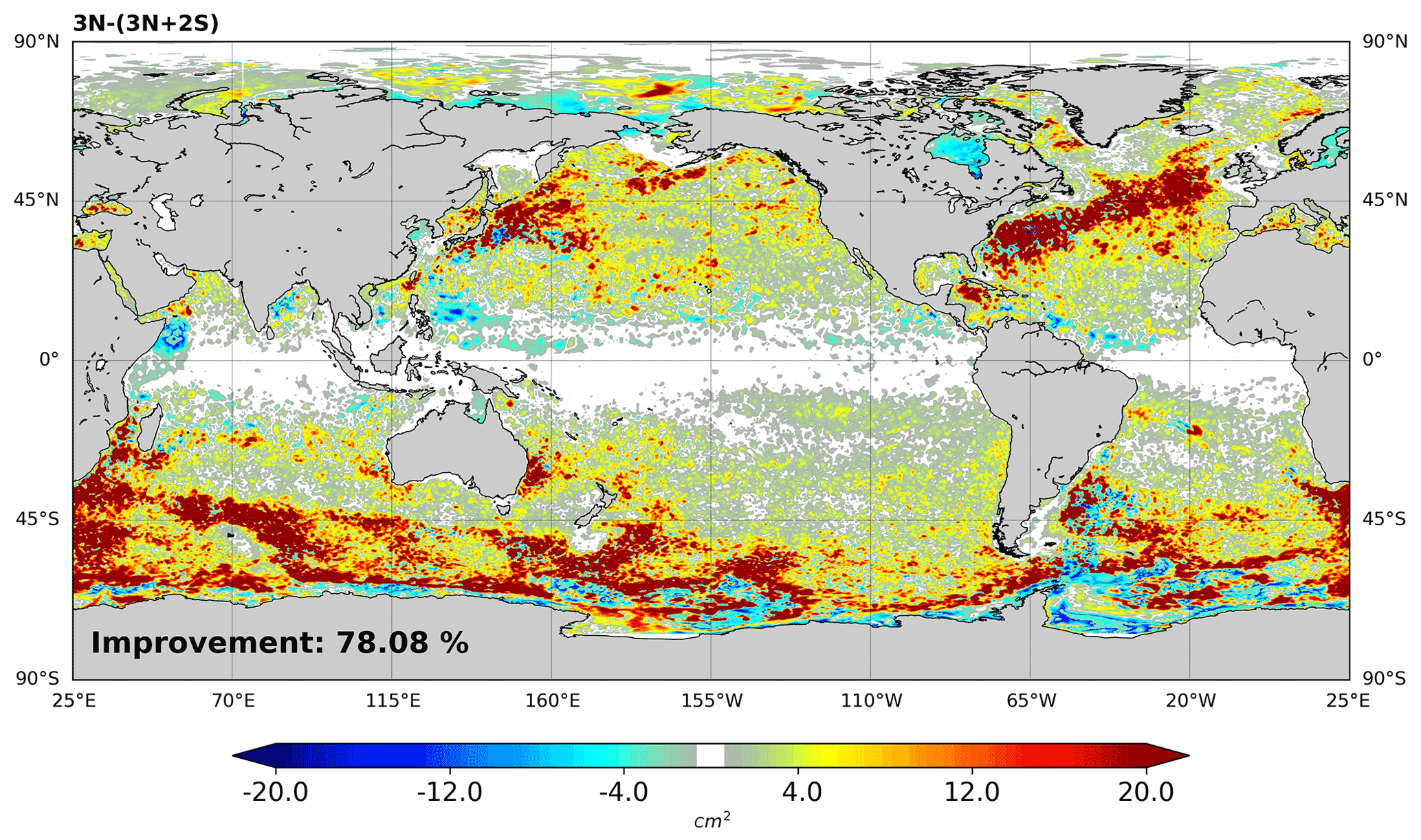
Figure 6Difference between analysis error variance of assimilation with three nadirs (3N) and assimilation of three nadirs and two wide-swath altimeters (3N + 2S).
Table 2SSH ocean analysis and forecast error statistics during the year 2015. Columns 1 and 2 represent the analysis and forecast variance of error computed from the difference between the OSSE and the NR (VarError, cm2). Columns 3 and 4 show the OSSEs error variance relative the FR error variance (Var*, %).
To better quantify the impact of swath data in the global system, errors are characterized for specific time and space scales. Figure 7 compares the error variance of the different OSSEs for wavelengths smaller than 200 km. The assimilation of nadir altimeters (Fig. 7b) already considerably reduces these errors compared to the FR. The addition of the swath altimeter assimilation (Fig. 7c) brought a major improvement for the regions where large errors remained (small scales) with the assimilation of nadir data. This improvement is prominent in the Gulf Stream, Kuroshio and ACC.
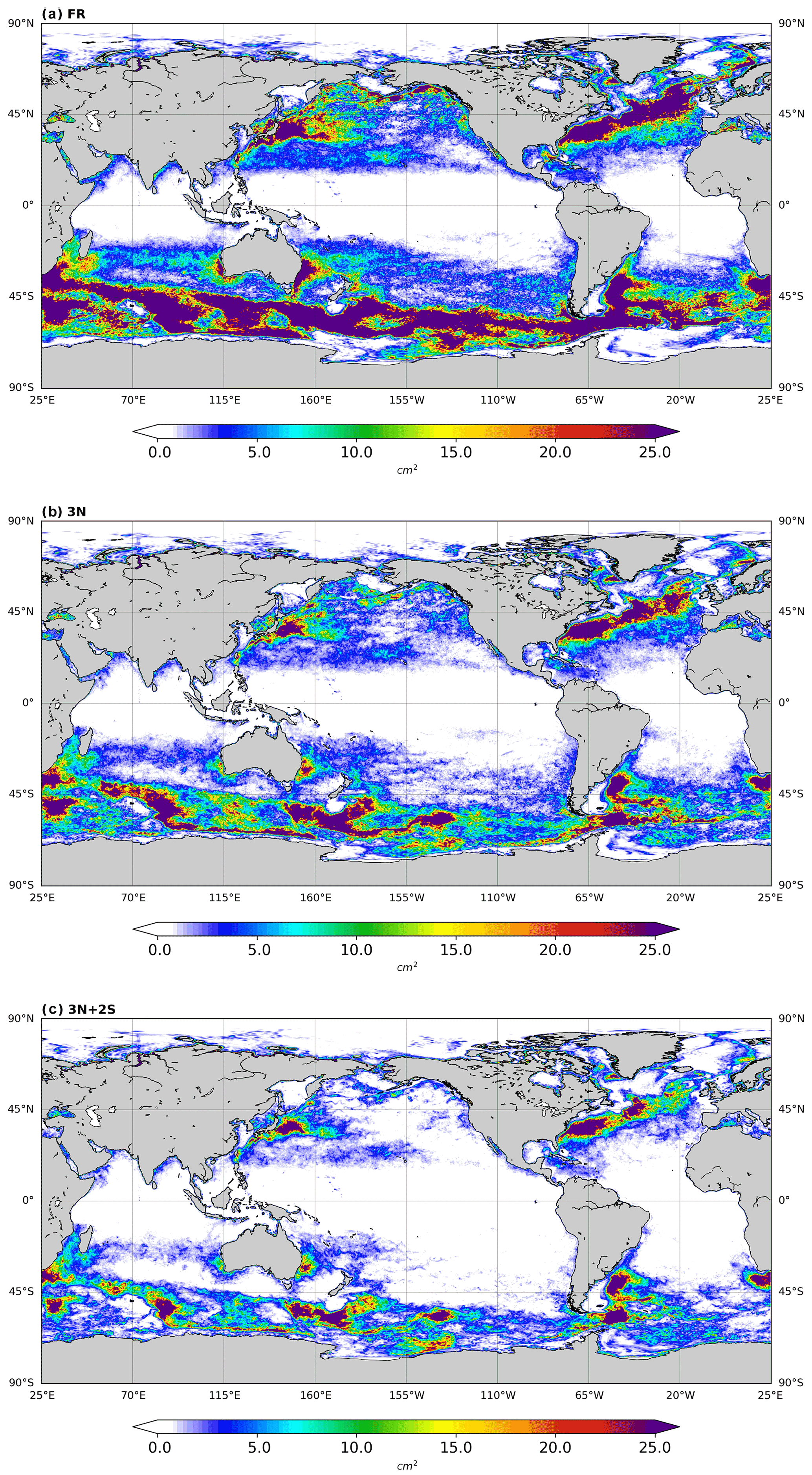
Figure 7Global maps of SSH analysis error (NR – model analysis; wavelengths <200 km) variance (in cm2, 2015). (a) Free run (FR); (b) with three nadirs (3N); (c) with three nadir and two wide-swath instruments (3N + 2S).
Figure 8 similarly compares these errors for periods of less than 20 d. The aim is to analyse the impact of wide-swath altimeter data on fast signals. Much of the error is corrected by assimilating the swath data in addition to the nadir data (Fig. 8c) compared to the nadir data alone (Fig. 8b). This improvement is visible throughout the global ocean. This shows that there is better control of the high-frequency signals when assimilating swath altimeter data as opposed to nadir data.
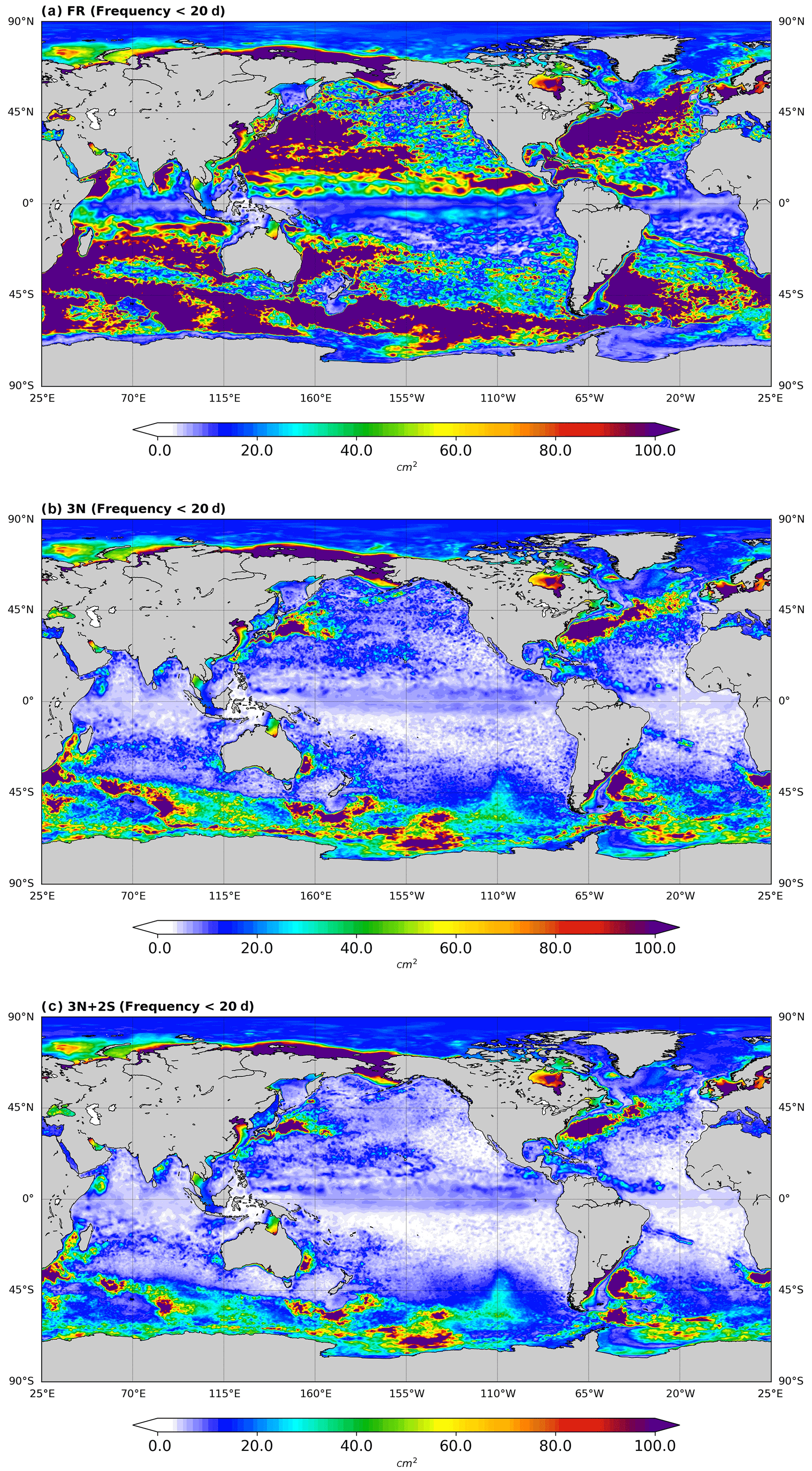
Figure 8Global maps of SSH analysis error (NR – model analysis; timescales <20 d) variance (in cm2, 2015). (a) Free run (FR); (b) with three nadirs (3N); (c) with three nadir and two wide-swath instruments (3N + 2S).
Figure 9 summarizes the main results of these analyses. The three panels of Fig. 9 represent the mean error variance as a function of latitude for the total error, the error for wavelengths <200 km and the error for periods <20 d. The swath altimeter data assimilation reduces the error at each latitude (red curves on the panels). This improvement is more pronounced at middle and high latitudes than at low latitudes. The impact on the western boundary currents and ACC currents is more evident at the mesoscale (<200 km) than at frequencies below 20 d.
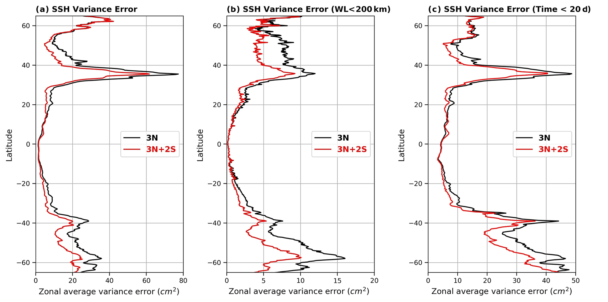
Figure 9The zonal SSH averaged error variance: (a) for full scales, (b) for scales less than 200 km and (c) for timescales less than 20 d; assimilation of 3N (black lines) and assimilation of 3N + 2S (red lines). Units are cm2.
4.2 Spectral analysis and coherence
Wavenumber power spectral density (PSD) and spatial and temporal coherence for each OSSE are discussed in this section. Spectra and coherence on boxes covering 10∘ in latitude by 20∘ in longitude at different latitudes (boxes in Fig. 3) are computed. Spectra were also computed on the same box (North Atlantic Drift: 19–10∘ W; 46–55∘ N, Box D, Fig. 3) as that presented by Bonaduce et al. (2018), using a regional model (IBI: Iberian–Biscay–Irish region) to make comparisons.
Figure 10 shows the power spectra of the SSH error in a variance-preserving form (Thomson and Emery, 2014) in the different boxes. The assimilation of nadir altimeter data (black curves) reduces the error at different scales compared to the FR (orange curves) except in region A (low-latitude, Fig. 10a) where the assimilation of nadir data introduces noise in the 50–200 km wavelength band. This is mainly due to the weak signal in these regions and the limited space–time sampling of the nadir altimeter constellation at these wavelengths. The assimilation has difficulty extrapolating the small-scale structures between the tracks (see discussion in Sect. 3.4.1 of Lellouche et al., 2018). The contribution of the swath altimeter data contributes to a clear reduction in the wavelength error spectra between 50 and 100 km depending on the latitude.
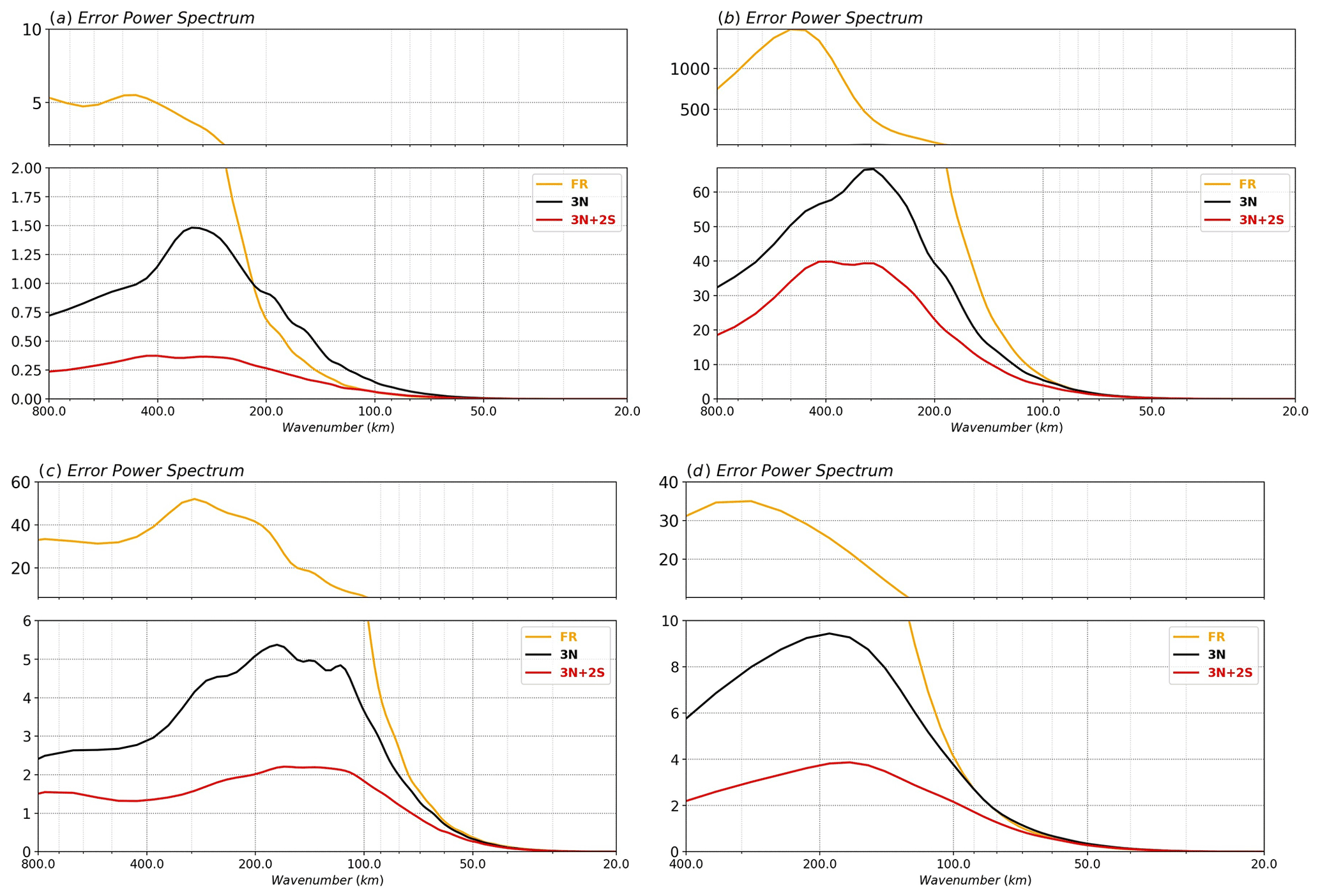
Figure 10Power spectra SSH error with respect to the NR; the spectra are shown in a variance preserving form (cm2), (a) low-latitude region (red box in Fig. 3), (b) Agulhas current (orange box in Fig. 3), (c) North Atlantic (high-latitude, green box in Fig. 3) and (d) North Atlantic Drift current (black box in Fig. 3).
The reduction of the error at the different wavelengths (ERspec) is defined as the percentage of the error with respect to FR (OSSE0). In all these areas (boxes) the assimilation of nadir altimeters (black curves) reduces the ERspec error by more than 65 % between 200 and 600 km. A major contribution is observed with swath altimeter data, as error reduction exceeds 90 % between 200 and 600 km over these regions (red curves, ERspec>90 %).
Spectral coherence analysis (temporal and spatial) is also performed to highlight the impact of assimilating swath data at different scales with respect to the NR. Coherence is defined as the correlation between two signals as a function of wavelengths (Ubelmann et al., 2015; Ponte and Klein, 2013; Klein et al., 2004). This coherence between the NR and different OSSEs is defined as follows:
where Crs and S represent the cross-spectral density and spectral density, respectively, and j refers to the experiment. The impact of the swath data is clear over all these regions (different latitudes) from 50 km of wavelength (red curves on the Fig. 11). The wavelengths and periods with a coherence of 0.5 (dotted line on the figures), which are usually taken as an estimation of the effective resolution (e.g. Ubelmann et al., 2015; Tchonang et al., 2021), show that wide-swath altimeter data (red lines) will provide much-improved insight into mesoscale ocean dynamics as compared with nadir altimeter data (black lines). In box D (Fig. 11d), which represents the North Atlantic Drift (the same box as that presented in Bonaduce et al., 2018), the wide-swath altimeter gain in the effective resolution is in the region of 60 % (105 km instead of 165 km for nadir altimeters). At low latitudes (box A, Fig. 11a), there is an improvement of around 80 % thanks to wide-swath altimeter data. This improvement is also observed at high latitudes (Fig. 11b and c), but it is less pronounced.

Figure 11Wavenumber spectral coherence with respect to the NR, (a) low-latitude region (red box in Fig. 3), (b) Agulhas current (orange box in Fig. 3), (c) North Atlantic (high-latitude, green box in Fig. 3) and (d) North Atlantic Drift current (black box in Fig. 3).
Figure 12 shows the time coherence for the four selected regions. The calculation of this coherence was based on filtered SSH fields of scales greater than 500 km to avoid the impact of large-scale and high-frequency signals on the results. At different latitudes (regions shown), wide-swath altimeter data improved the temporal coherence with the NR compared to the nadir data. The effective time resolution in regions A and B (Fig. 12a and b) is 20 d for wide-swath altimeters instead of 40 d for nadir altimeters (half the time). At middle and high latitudes (Fig. 12c: Gulf Stream and Fig. 12d: North Atlantic Drift), there is a strong improvement, with a time resolution of 25 d for wide-swath altimeters, whereas with the nadir altimeter data the consistency reaches 50 % around 50 d.
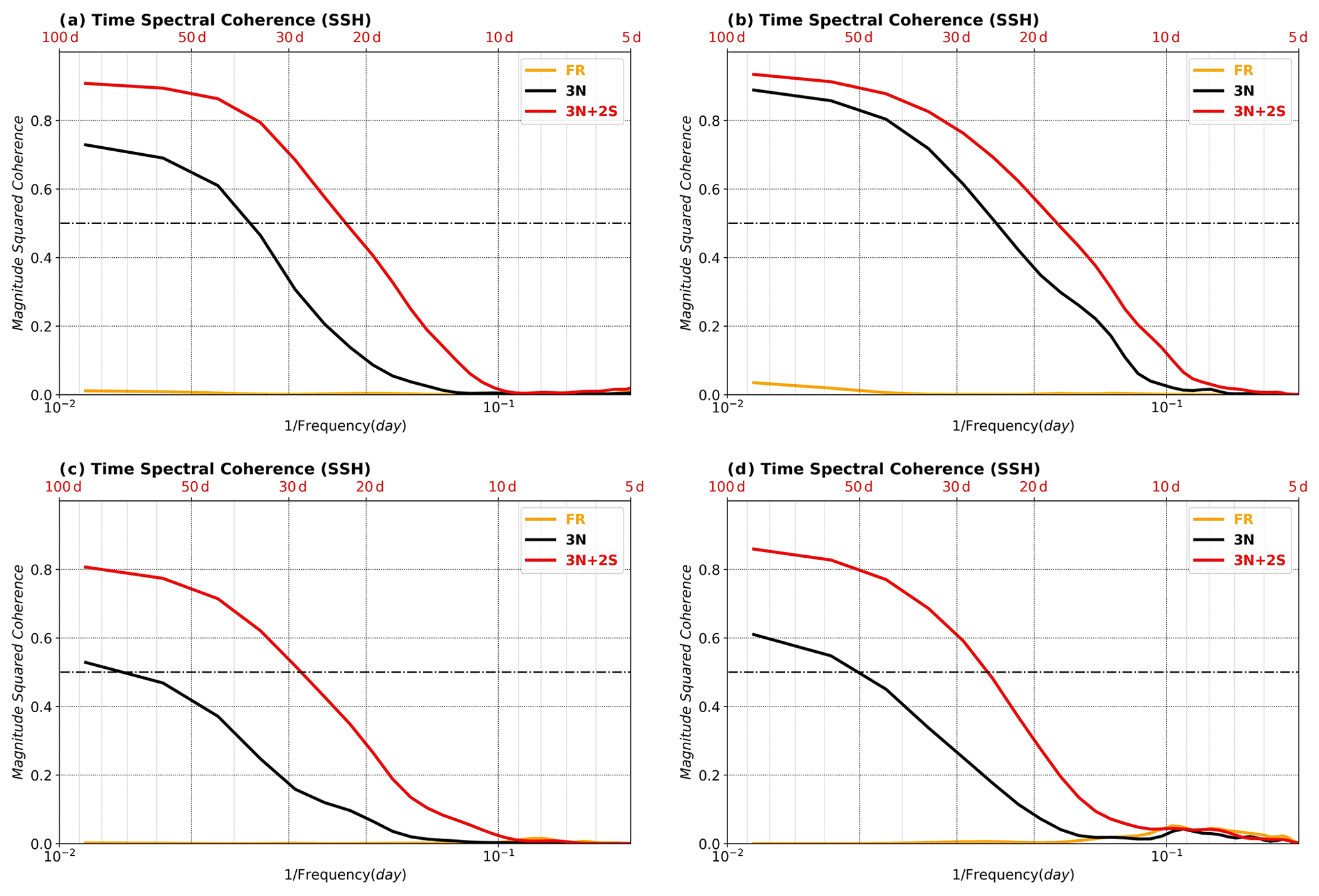
Figure 12Time spectral coherence with respect to the NR (wavelengths <500 km), (a) low-latitude region (red box), (b) Agulhas current (orange box), (c) North Atlantic (high-latitude, green box) and (d) North Atlantic Drift current (black box).
4.3 Impact on temperature, salinity and zonal velocities
Figure 13 shows the variance of the temperature and salinity error (NR-OSSEs) as a function of depth for the global ocean. The temperature error profile shows a maximum at about 100 m depth, which represents the thermocline. This error is significantly reduced by assimilating the nadir altimeter data (black profile) compared to the free model (FR, orange profile). The assimilation of the wide-swath altimeter data does not degrade this score and we even have a slight improvement between 100 and 750 m depth. For salinity (Fig. 13b), the improvement is less clear, but no degradation is observed at any depth.
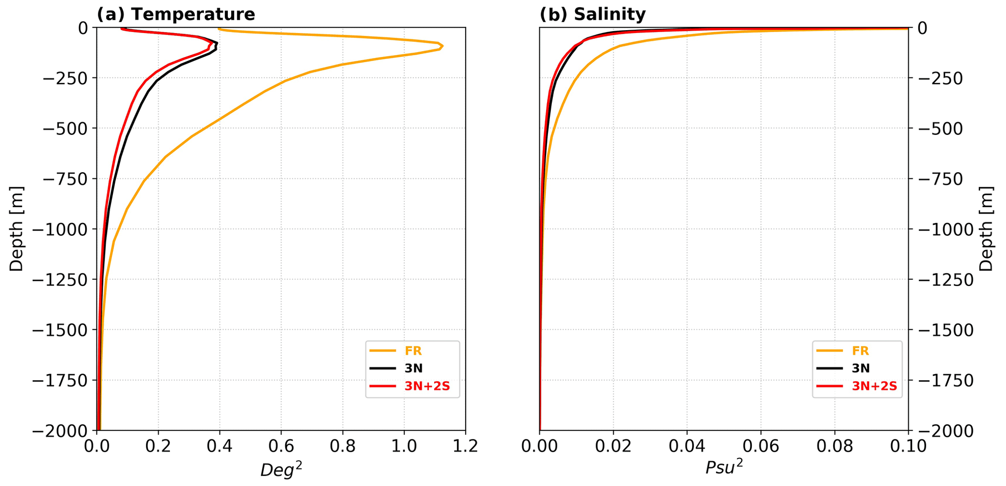
Figure 13Global averaged error variance: (a) temperature (in Deg2) and (b) salinity (Psu2) over the period of March to December 2015. The results were obtained by comparing the zonal and meridional velocities of OSSEs with the NR; FR (orange lines), 3N (black lines) and 3N + 2S (red lines).
Figure 14 similarly shows the average error variance of both the zonal (U) and meridional (V) velocity as a function of depth for the global ocean for each of the experiments. The assimilation of nadir altimeter data (black profiles) brings a significant reduction of this error with respect to the FR (orange profiles) between the surface and 1000 m depth on both U and V. There is a clear reduction over the whole depth with the wide-swath altimeter data assimilation (red profiles) on both velocity components. Similarly, Fig. 15 compares the evolution of the velocity error variance as a function of time over the year 2015 at the surface and at 300 m depth. On the surface (top panels), there is a constant improvement (red curves) on both components (U and V). On the other hand, at 300 m depth, there is a reduction that sets in after 1 month and remains constant over the year. Table 3 summarizes the statistics on the horizonal velocities from Fig. 15. Overall, there is an error reduction of more than 30 % for the surface currents and more than 50 % for the currents at 300 m with wide-swath altimeter data. Wide-swath altimeter (2D) data allow a much better constraint of the ocean dynamics compared to the assimilation of nadir data.

Figure 14Global averaged error variance (in cm2 s−2): (a) zonal velocity and (b) meridional velocity over the period of March to December 2015. The results were obtained by comparing the zonal and meridional velocities of OSSEs with the NR; FR (orange lines), OSSE1 (3N; black lines) and OSSE2 (3N + 2S; red lines).
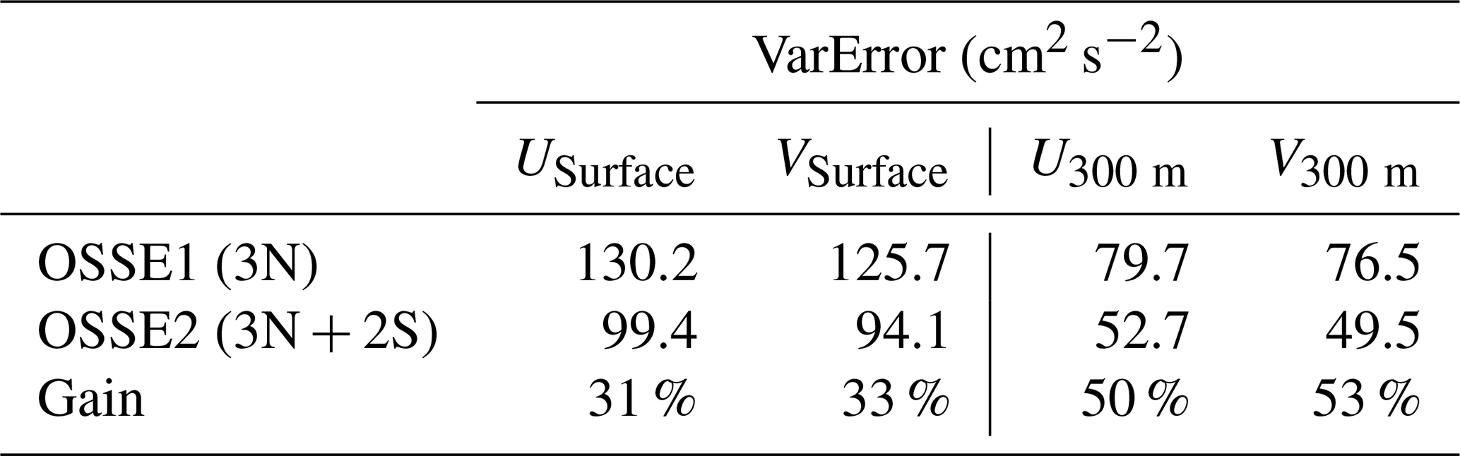
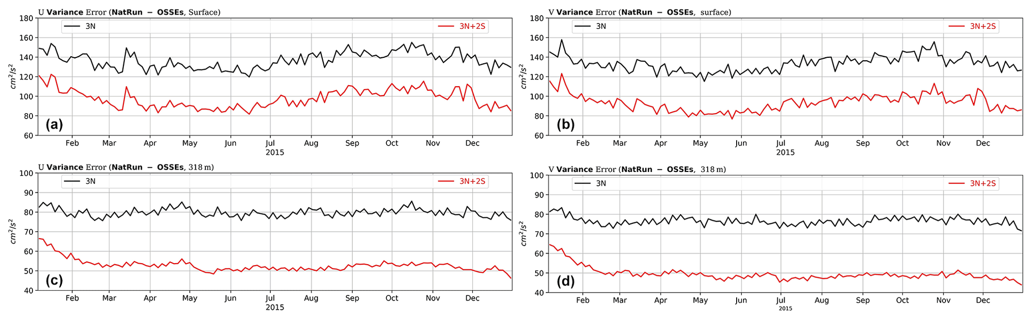
Figure 15Temporal evolution of zonal and meridional velocity error variance (cm2 s−2) for 7 d ocean analysis over the period from 1 January to 20 December 2015. The results were obtained by comparing both components of the velocity (U,V) to that of the NR. Black curves with assimilation of nadir altimeters (3N) and red curves with assimilation of nadirs and wide-swath instruments (3N + 2S). (a) and (b) Surface velocities and (c) and (d) velocities at 300 m depth. The statistics are summarized in Table 3.
The SWOT mission to be launched at the end of 2022 will demonstrate the potential of swath altimetry, which is likely to revolutionize our ability to monitor and forecast ocean dynamics from mesoscale to submesocale. SWOT will considerably improve on the capabilities of the present constellation of nadir altimeters (Benkiran et al., 2021; Tchonang et al., 2021), but its time sampling (21 d) will be a limitation. A constellation of two wide-swath altimeters will provide, however, much better space–time sampling and should allow us to observe 68 % of the ocean every 50 km and 5 d (CNES, 2020). Such a configuration is envisioned by ESA for the long-term evolution (post-2030) of the Copernicus Sentinel 3 topography mission to meet the requirements expressed by the Copernicus Marine Service and its applications (CMEMS, 2017). To quantify the expected performances, a series of OSSEs have been carried out in this study using a state-of-the-art high-resolution (∘) global ocean data assimilation system.
Results suggest the high potential of such a configuration and should provide a major improvement of our capabilities to monitor and forecast the oceans. Compared to the present situation with three nadir altimeters flying simultaneously (Sentinel 6 and the two Sentinel 3 instruments), the SSH analysis and 7 d forecast error will be globally reduced by almost 50 %. Improvements are much larger in middle- and high-latitude regions and smaller in tropical and equatorial regions in the OSSEs. Surface and deep velocity fields will also be greatly improved. Surface current forecast errors should be equivalent to today's surface current analysis errors or alternatively will be improved (error variance reduction) by 30 % at the surface and 50 % for 300 m depths.
The resolution capabilities will be drastically improved and will be closer to 100 km wavelength as opposed to today where they are above 250 km (on average). On average, on the four boxes presented (representative of different latitudes), there is a 60 % improvement of the resolved structures with the two wide-swath altimeters in the OSSEs. In terms of timescales resolved, improvements will be larger than expected for time periods around 20 d (50 % of coherence, improvements of 60 %).
Flying a constellation of two wide-swath altimeters thus looks to be a very promising solution for the long-term evolution of the Sentinel 3 constellation and the Copernicus Marine Service.
Follow-up studies should consider the full error spectrum taking into account, in particular, correlated long wavelength errors inherent to altimeter wide-swath techniques (e.g. roll errors). This will first require better specification of these errors given the instrument and platform designs and the assessment of the impact of techniques that will be used to reduce them. As demonstrated by a series of studies carried out for the preparation of the SWOT mission (e.g. Dibarboure and Ubelmann, 2014), techniques such as swath–swath and swath–nadir cross-over minimization will allow a large part of these errors to be reduced. We thus plan to carry out more advanced OSSEs that take into account the full error spectrum of wide-swath altimeters, the reduction of these errors through cross-calibration techniques, and the assimilation of corrected data and their residual (correlated) errors in advanced data assimilation schemes.
The assimilation code used for this study is the operational code of Mercator Ocean International which is not yet distributed, the code of the NEMO model is available on https://doi.org/10.5281/zenodo.6334656 (Gurvan et al., 2022).
Data are available upon request to the authors.
MB set up the scientific protocol of OSSEs, performed the simulation and made the analyses of the results. PYLT and GD wrote the introduction and contributed to the scientific and analysis of the results.
The contact author has declared that neither they nor their co-authors have any competing interests.
Publisher’s note: Copernicus Publications remains neutral with regard to jurisdictional claims in published maps and institutional affiliations.
The study was funded by ESA and was also carried out as part of a partnership agreement between Mercator Ocean International and CNES. All participants in the WiSA study are thanked for their high-quality work.
This research has been supported by the CNES (grant no. 2017-0003803).
This paper was edited by Andrew Moore and reviewed by two anonymous referees.
Adcroft, A. and Campin, J. M.: Rescaled height coordinates for accurate representation of free-surface flows in ocean circulation models, Ocean Modell., 7, 269–284, ISSN 1463-5003, https://doi.org/10.1016/j.ocemod.2003.09.003, 2004.
Benkiran, M., Ruggiero, G., Greiner, E., Le Traon, P. Y., Rémy, E., Lellouche, J. M., Bourdallé-Badie, R., Drillet, Y., and Tchonang, B.: Assessing the impact of the assimilation of SWOT observations in a global high-resolution analysis and forecasting system. Part 1: method, Frontiers in Marine Science, 8, 691955, https://doi.org/10.3389/fmars.2021.691955, 2021.
Bidlot, J.-R.: Impact of ocean surface currents on the ECMWF forecasting system for atmosphere circulation and ocean waves, in: GlobCurrent Preliminary User Consultation Meeting, Brest, 7–9 March 2012, https://cersat.ifremer.fr/content/download/144880/file/1505_Bidlot.pdf, last access: 20 September 2012.
Blanke, B. and Delecluse, P.: Variability of the tropical Atlantic-Ocean simulated by a general-circulation model with 2 different mixed-layer physics, J. Phys. Oceanogr., 23, 1363–1388, https://doi.org/10.1175/1520-0485(1993)023<1363:VOTTAO>2.0.CO;2, 1993.
Bonaduce, A., Benkiran, M., Remy, E., Le Traon, P. Y., and Garric, G.: Contribution of future wide-swath altimetry missions to ocean analysis and forecasting, Ocean Sci., 14, 1405–1421, https://doi.org/10.5194/os-14-1405-2018, 2018.
Brodeau, L., Barnier, B., Gulev, S. K., and Woods, C.: Climatologically significant effects of some approximations in the bulk parameterizations of turbulent air–sea fluxes, J. Phys. Oceanogr., 47, 5–28, https://doi.org/10.1175/JPO-D-16-0169.1, 2017.
Chelton, D. B., Ries, J. C., Haines, B. J, Fu, L. L, and Callahan, P. S.: Satellite Altimetry, in: Satellite Altimetry and Earth Sciences: A Handbook of Techniques and Applications, edited by: Fu, L. L. and Cazenave, A., Academic: San Diego, CA, USA, 2001, 69, 1–131, https://doi.org/10.1016/S0074-6142(01)80146-7, 2001.
CMEMS: CMEMS requirements for the evolution of the Copernicus Satellite Component https://marine.copernicus.eu/sites/default/files/media/pdf/2020-10/CMEMS-requirements-satellites.pdf, last access: 21 February 2017.
CNES: Phase A WiSA: a Wide Swath Altimetry mission for high resolution oceanography and hydrology, Final report, DSO/SI/IP-2019.19671, 2020.
Dee, D. P., Uppala, S. M., Simmons, A. J., Berrisford, P., Poli, P., Kobayashi, S., Andrae, U., Balmaseda, M. A., Balsamo, G., Bauer, P., Bechtold, P., Beljaars, A. C. M., van de Berg, L., Bidlot, J., Bormann, N., Delsol, C., Dragani, R., Fuentes, M., Geer, A. J., Haimberger, L., Healy, S. B., Hersbach, H., Hólm, E. V., Isaksen, L., Kållberg, P., Köhler, M., Matricardi, M., McNally, A. P., Monge-Sanz, B. M., Morcrette, J.-J., Park, B.-K., Peubey, C., de Rosnay, P., Tavolato, C., Thépaut, J.-N., and Vitart, F.: The ERA-Interim reanalysis: configuration and performance of the data assimilation system, Q. J. R. Meteorol. Soc., 137, 553–597, https://doi.org/10.1002/qj.828, 2011.
Dibarboure, G. and Ubelmann, C.: Investigating the Performance of Four Empirical Cross-Calibration Methods for the Proposed SWOT Mission, Remote Sensing, 6, 4831–4869, 2014.
Dibarboure, G., Lamy, A., Pujol, M. I., and Jettou, G.: The drifting phase of SARAL: Securing stable ocean mesoscale sampling with an unmaintained decaying altitude, Remote Sensing, 10, 1051, https://doi.org/10.3390/rs10071051, 2018.
Errico, R. M., Yang, R., Privé, N. C., Tai, K.-S., Todling, R., Sienkiewicz, M. E., and Guo, J.: Development and validation of observing-system simulation experiments at NASA's Global Modeling and Assimilation Office, Q. J. Roy. Meteorol. Soc., 139, 1162–1178, https://doi.org/10.1002/qj.2027, 2013.
Esteban-Fernandez, D.: SWOT project: Mission performance and error budget, JPL Doc, JPL D-79084, 83 pp., https://doi.org/10.1109/IGARSS.2018.8517385, 2013.
Gaultier, L., Ubelmann, C., and Fu, L. L.: The Challenge of Using Future SWOT Data for Oceanic Field Reconstruction, J. Atmos. Ocean. Tech., 33, 119–126, https://doi.org/10.1175/JTECH-D-15-0160.1, 2016.
Gurvan, M., Bourdallé-Badie, R., Chanut, J., Clementi, E., Coward, A., Ethé, C., Iovino, D., Lea, D., Lévy, C., Lovato, T., Martin, N., Masson, S., Mocavero, S., Rousset, C., Storkey, D., Müller, S., Nurser, G., Bell, M., Samson, G., and Moulin, A.: NEMO ocean engine, In Notes du Pôle de modélisation de l'Institut Pierre-Simon Laplace (IPSL) (v4.2.0, Number 27), Zenodo [code], https://doi.org/10.5281/zenodo.6334656, 2022.
Hamon M., Greiner E., Le Traon P. Y., and Remy E.: Impact of multiple altimeter data and mean dynamic topography in a global analysis and forecasting system, J. Atmos. Ocean. Tech., 36, 1255–1266, https://doi.org/10.1175/JTECH-D-18-0236.1, 2019.
Klein, P., Lapeyre, G., and Large, W. G.: Wind ringing of the ocean in presence of mesoscale eddies, Geophys. Res. Lett., 31, l15306, https://doi.org/10.1029/2004GL020274, 2004.
Lamy, A. and Albouys, V.: Mission design for the SWOT mission, in: Proceedings of the 2014 International Symposium on Space Flight Dynamics (ISSFD) meeting, Laurel, Maryland, USA, 5–9 May 2014, https://issfd.org/ISSFD_2014/ISSFD24_Paper_S17-1_LAMY.pdf (last access: 09 May 2014), 2014.
Large, W. G. and Yeager, S. G.: The global climatology of an interannually varying air–sea flux data set, Clim. Dynam., 33, 341–364, https://doi.org/10.1007/s00382-008-0441-3, 2009.
Lellouche, J.-M., Le Galloudec, O., Drévillon, M., Régnier, C., Greiner, E., Garric, G., Ferry, N., Desportes, C., Testut, C.-E., Bricaud, C., Bourdallé-Badie, R., Tranchant, B., Benkiran, M., Drillet, Y., Daudin, A., and De Nicola, C.: Evaluation of global monitoring and forecasting systems at Mercator Océan, Ocean Sci., 9, 57–81, https://doi.org/10.5194/os-9-57-2013, 2013.
Lellouche, J.-M., Greiner, E., Le Galloudec, O., Garric, G., Regnier, C., Drevillon, M., Benkiran, M., Testut, C.-E., Bourdalle-Badie, R., Gasparin, F., Hernandez, O., Levier, B., Drillet, Y., Remy, E., and Le Traon, P.-Y.: Recent updates to the Copernicus Marine Service global ocean monitoring and forecasting real-time ∘ high-resolution system, Ocean Sci., 14, 1093–1126, https://doi.org/10.5194/os-14-1093-2018, 2018.
Le Traon, P. Y., Dibarboure, G., Jacobs, G., Martin, M., Remy, E., and Schiller, A.: Use of satellite altimetry for operational oceanography, in: Satellite Altimetry Over Oceans and Land Surfaces, 1st edn., edited by: Stammer, D., and Cazenave, A., CRC Press, Taylor, 28 p., ISBN: 9781315151779, 2017.
Le Traon, P.-Y., Reppucci, A., Alvarez Fanjul, E., et al.: The Copernicus Marine Service perspective, Frontiers in Marine Science, 6, 22 p., https://doi.org/10.3389/fmars.2019.00234, 2019.
Le Traon, P. Y., Abadie, V., Ali, A., et al.: The Copernicus Marine Service from 2015 to 2021: six years of achievements, Special Issue Mercator Ocean Journal, 57, 220 p., https://doi.org/10.48670/moi-cafr-n813, 2021.
Madec, G. and The NEMO Team: NEMO ocean engine, Note du Pôle de mod elisation, Institut Pierre-Simon Laplace (IPSL), France, 27, ISSN 1288–1619, 2008.
Morrow, R., Fu, L. L., Ardhuin, F., Benkiran, M., Chapron, B., Cosme, E., d’Ovidio, F., Farrar, J. T., Gille, S. T., Lapeyre, G., Le Traon, P.-Y., Pascual, A., Ponte, A., Qiu, B., Rascle, N., Ubelmann, C., Wang, J., and Zaron, E. D.: Global observations of fine-scale ocean surface topography with the surface water and ocean topography (SWOT) mission, Frontiers in Marine Science, 6, 232, https://doi.org/10.3389/fmars.2019.00232, 2019.
Ponte, A. L. and Klein, P.: Reconstruction of the upper ocean 3D dynamics from high-resolution sea surface height, Ocean Dynam., 63, 777–791, https://doi.org/10.1007/s10236-013-0611-7, 2013.
Rodi, W.: Examples of calculation methods for flow andmixing in stratified fluids, J. Geophys. Res., 92, 5305–5328, https://doi.org/10.1029/JC092iC05p05305, 1987.
Roullet, G. and Madec, G.: Salt conservation, free surface, and varying levels: a new formulation for ocean general circulation models, J. Geophys. Res., 105, 23927–23942, 2000.
Shchepetkin, A. F. and McWilliams, J. C.: The Regional Oceanic Modeling System (ROMS): A split-explicit, free-surface, topography-following-coordinate ocean model, Ocean Modell., 9, 347–404, https://doi.org/10.1016/j.ocemod.2004.08.002, 2005.
Shchepetkin A. F. and McWilliams J. M.: Computational Kernel Algorithms for Fine-Scale, Multiprocess, Longtime Oceanic Simulations, Handbook of Numerical Analysis, Elsevier, 14, 121–183, ISSN: 1570-8659, ISBN: 9780444518934, https://doi.org/10.1016/S1570-8659(08)01202-0, 2009.
Tchonang, C. B., Benkiran, M., Le Traon, P. Y., Van Gennip, S., Lellouche, J. M., and Ruggiero, G.: Assessing the impact of the assimilation of SWOT observations in a global high-resolution analysis and forecasting system. Part 2: Results, Frontiers in Marine Science, https://doi.org/10.3389/fmars.2021.687414, 2021.
Thomson, R. E. and Emery, W. J.: Chapter 5 – Time Series Analysis Methods, in: Data Analysis Methods in Physical Oceanography, 3rd edn., edited by: Thomson, R. E. and Emery, W. J., Elsevier, Boston, 425–591, https://doi.org/10.1016/B978-0-12-387782-6.00005-3, 2014.
Ubelmann, C., Klein, P., and Fu, L.-L.: Dynamic Interpolation of Sea Surface Height and Potential Applications for Future High-Resolution Altimetry Mapping, J. Atmos. Ocean. Tech., 32, 177–184, https://doi.org/10.1175/JTECH-D-14-00152.1, 2015.
Vergara, O., Morrow, R., Pujol, I., Dibarboure, G., and Ubelmann, C.: Revised global wave number spectra from recent altimeter observations, J. Geophys. Res.-Oceans, 124, 3523–3537, 2019.