Sea-level variability and change along the Norwegian coast between 2003 and 2018 from satellite altimetry, tide gauges, and hydrography

Sea-level variations in coastal areas can differ significantly from those in the nearby open ocean. Monitoring coastal sea-level variations is therefore crucial to understand how climate variability can affect the densely populated coastal regions of the globe. In this paper, we study the sea-level variability along the coast of Norway by means of in situ records, satellite altimetry data, and a network of eight hydrographic stations over a period spanning 16 years (from 2003 to 2018). At first, we evaluate the performance of the ALES-reprocessed coastal altimetry dataset (1 Hz posting rate) by comparing it with the sea-level anomaly from tide gauges over a range of timescales, which include the long-term trend, the annual cycle, and the detrended and deseasoned sea-level anomaly. We find that coastal altimetry and conventional altimetry products perform similarly along the Norwegian coast. However, the agreement with tide gauges in terms of trends is on average 6 % better when we use the ALES coastal altimetry data. We later assess the steric contribution to the sea level along the Norwegian coast. While longer time series are necessary to evaluate the steric contribution to the sea-level trends, we find that the sea-level annual cycle is more affected by variations in temperature than in salinity and that both temperature and salinity give a comparable contribution to the detrended and deseasoned sea-level variability along the entire Norwegian coast. A conclusion from our study is that coastal regions poorly covered by tide gauges can benefit from our satellite-based approach to study and monitor sea-level change and variability.

1 Introduction

Global mean sea level (GMSL) has been rising during the XX century and the beginning of the XXI century at a rate of approximately 1.5 mm yr⁻¹ (Frederikse et al., 2020). Its rise is projected to continue, and even accelerate, in the future (Hermans et al., 2021), thus posing significant stress on coastal communities (Nicholls, 2011). At a local scale, though, sea-level variations can largely depart from the global average (Stammer et al., 2013). Therefore, accurate estimation and attribution of sea-level rise at regional scale are among the major challenges of climate research (Frederikse et al., 2018), with large societal benefit and impact due to the large human population living in coastal areas (e.g. Lichter et al., 2011). The Norwegian coast is no exception. While it appears less vulnerable to sea-level variations because of its steep topography and rocks resistant to erosion, it has a large number of coastal cities, most of which have undergone significant urban development in recent times (Simpson et al., 2015).

Since August 1992, when NASA and CNES launched the TOPEX/Poseidon mission, satellite altimetry has enormously expanded our knowledge of the ocean and the climate system (e.g. Cazenave et al., 2018). With the help of satellite altimetry, oceanographers and climate scientists could observe sea-level variations over almost the entire ocean (e.g. Nerem et al., 2010; Madsen et al., 2019) and understand their causes (e.g. Richter et al., 2020), detect ocean currents (e.g. Zhang et al., 2007) and monitor their variability (e.g. Chafik et al., 2015), and observe the evolution of climate events (e.g. Ji et al., 2000) and investigate their origins (e.g. Picaut et al., 2002). Satellite altimetry has made these, and other achievements, possible because it has provided continuous sea-level observations over large parts of the ocean in areas where sea-level measurements were previously only occasional.

While invaluable over the open ocean, satellite altimetry measurements have historically been flagged as unreliable in coastal areas (e.g. Benveniste et al., 2020). Indeed, the accuracy of radar altimetry, which is 2–3 cm over the open ocean (e.g. Volkov and Pujol, 2012), deteriorates in coastal regions because of technical issues (e.g. Xu et al., 2019). Notably, large variations in the backscattering of the area illuminated by the radar altimeters (for example, due to the presence of land or to patches of very calm water in sheltered areas; Gómez-Enri et al., 2010) contaminate the returned echoes of radar altimeters, and the complex topography of continental shelves, together with the irregular shape of most coastlines, makes geophysical corrections in coastal areas less accurate than in the open ocean.

To increase the accuracy of radar altimetry in coastal regions, Passaro et al. (2014) have developed the Adaptive Leading Edge Subwaveform (ALES) retracking algorithm. The ALES retracker addresses the altimeter footprint contamination issue by avoiding echoes from bright targets (e.g. land). Several studies have found a clear improvement of the ALES-reprocessed satellite altimetry observations over conventional altimetry products in different areas of the world (e.g. Passaro et al., 2014, 2015, 2016, 2018, 2021), with the new algorithm providing estimates of the altimetry parameters in coastal areas with levels of accuracy typical of the open ocean for distances to the coast of up to circa 3 km (e.g. Passaro et al., 2014).

In this paper, we investigate how the ALES-reprocessed satellite altimetry dataset resolves sea level along the coast of Norway compared to all the tide-gauge records available over the 16-year period between 2003 and 2018. Indeed, to the best of our knowledge, previous validation studies have not considered the entire Norwegian coast but only parts of it: Passaro et al. (2015) focused on the transition zone between the North Sea and the Baltic Sea, whereas Rose et al. (2019) focused on Honningsvåg in northern Norway. The Norwegian coast also appears particularly interesting for validation purposes because, during the altimetry period, it is well covered by tide gauges and because conventional altimetry products have previously failed to reproduce the sea-level trends in the region (Breili et al., 2017). The present study will thus investigate the performance of ALES in relation to these issues.

We further use the ALES-reprocessed altimetry dataset in combination with a network of hydrographic stations along the coast of Norway to study the steric contribution to the sea-level variability in the region, which is known to be challenging at the regional scale (e.g. Raj et al., 2020; Richter et al., 2012). Richter et al. (2012) have already used tide gauges and hydrographic stations to assess the different contributions to the Norwegian sea-level variability between 1960 and 2010. However, compared to their study, we use the coastal altimetry dataset to reconstruct a monthly mean sea-level time series centred over each hydrographic station. This is an advantage over Richter et al. (2012) since some of the Norwegian tide gauges are located in sheltered areas and might not be representative of the variability captured by the nearest hydrographic station (which can be as far as 100 km apart). Moreover, compared to Richter et al. (2012), we analyse the annual cycle of the sea level in more detail by describing how its properties change along the Norwegian coast. Furthermore, sea-level measurements from satellite altimetry, unlike those from tide gauges, do not need to be corrected for vertical land motion.

This paper is organized as follows. Section 2 describes the data used in the coastal sea-level signal analysis. An analysis of sea-level components retrieved by each observational instrument is provided in Sect. 3. The coastal sea level from tide gauges and satellite altimetry is compared in terms of temporal variability and trends in Sect. 4. Section 5 focuses on the steric contribution to the sea-level estimates from altimetry, tide gauges, and hydrographic data. Section 6 summarizes and concludes.

2 Data

2.1 ALES-reprocessed multi-mission satellite altimetry

To provide more accurate sea-level estimates in coastal regions, the ALES retracker operates in two stages. At first, it fits the leading edge of the waveform to have a rough estimate of the significant wave height (SWH). Then, depending on the SWH, the algorithm selects a portion of the waveform (known as subwaveform) and fits it to estimate the range (the distance between the satellite and the sea surface), the SWH, and the backscatter coefficient.

The dataset is freely available on the Open Altimetry Database website of the Technische Universität München (https://openadb.dgfi.tum.de/en/, last access: 22 July 2020). The European Space Agency (ESA) also provides, through the Sea Level Climate Change Initiative Programme, a coastal satellite altimetry dataset reprocessed with the ALES retracker. However, it only covers the northern latitudes up to 60^∘ N and, therefore, only part of the region of interest in this study (Benveniste et al., 2020).

The dataset includes observations from the following altimetry missions: Envisat (version 3), Jason-1, Jason-1 extended mission, Jason-1 geodetic mission, Jason-2, Jason-2 extended mission, Jason-3, SARAL, and SARAL drifting phase. These are provided at a 1 Hz posting rate (equivalent to an along-track resolution of circa 7 km) and cover the period from June 2002 to April 2020, with the exception of one data gap between November 2010 (end of Envisat) and March 2013 (start of SARAL) to the north of 66^∘ N. Data from different missions have been cross-calibrated so that there are no inter-mission biases.

Prior to distribution, several corrections have been applied to the satellite altimetry data. Among them, the geophysical corrections are of particular interest for the purpose of this study. Indeed, to validate the ALES-reprocessed altimetry against the Norwegian tide gauges, the same physical signal must be removed from both datasets. The geophysical corrections applied to the ALES-reprocessed altimetry data include the tidal and the dynamic atmospheric corrections (COSTA user manual, http://epic.awi.de/43972/1/User_Manual_COSTA_v1_0.pdf, last access: 22 July 2020). The correction for ocean and pole tides has been performed using the EOT11a tidal model. The solid-Earth-related tides have also been subtracted from the orbital altitude but, as it leaves the altimetry data in sync with the tide gauges (which are based on the solid Earth), this correction has no further interest for this study. The dynamic atmospheric correction (DAC), available at https://www.aviso.altimetry.fr/index.php?id=1278 (last access: 12 April 2021), removes both the wind and the pressure contribution to the sea-level variability at timescales shorter than 20 d and only the pressure contribution to the sea-level variability at longer timescales. The high-frequency component of the DAC is computed using the Mog2D-G high-resolution barotropic model (Carrère and Lyard, 2003), and it is removed because it would otherwise alias the altimetry data. The low-frequency component accounts for the static response of the sea level to changes in pressure, a phenomenon also known as the inverse barometer effect (IBE), according to which a 1 hPa increase or decrease in sea-level pressure corresponds to a 1 cm decrease or increase in sea level. To validate the ALES-reprocessed altimetry against the Norwegian tide gauges, the relevant physical signals at the relevant timescales must be removed from the tide-gauge data (Sect. 2.2).

The producers of ALES flag some of the data as unreliable. More precisely, they recommend excluding observations that fall within a distance of 3 km from the coast and whose sea-level anomaly (SLA), SWH, and standard deviation exceed 2.5, 11, and 0.2 m, respectively. We have followed these recommendations with one exception: we have lowered the threshold on the sea-level anomaly from 2.5 to 1.5 m because this choice leads to better agreement between the tide gauges and the ALES altimetry dataset between Måløy and Rørvik along the west coast of Norway (Fig. 1).

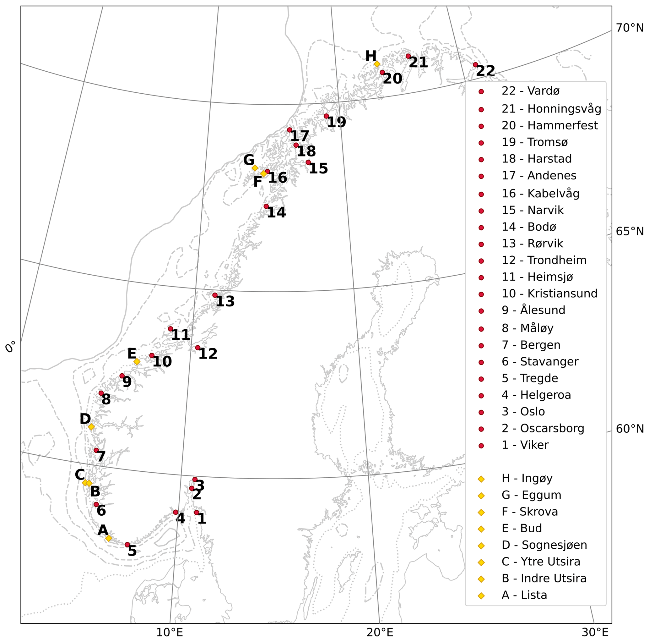
Figure 1 Location of the tide gauges and of the hydrographic stations considered in this study (red circles and yellow diamonds, respectively). The solid, dashed, dash-dotted, and dotted light gray lines indicate the 500, 300, 150, and 50 m isobaths, respectively.

2.2 Tide gauges

The Norwegian Mapping Authority (Kartverket) provides information on observed water levels at 24 permanent tide-gauge stations along the coast of Norway. Data are updated, referenced to a common datum, quality-checked, and freely distributed through a dedicated web API (http://api.sehavniva.no, last access: 28 April 2021).

Even though most tide gauges provide a few decades of sea-level measurements, in this study we only consider the period between January 2003 and December 2018 because it overlaps with the time window spanned by the ALES altimetry dataset. Moreover, we only select 22 of the 24 permanent tide gauges available: we exclude Mausund, since it has no measurements available before November 2010, and Ny-Ålesund because it is outside our region of interest.

Over the period considered, the only tide gauges with missing values are Heimsjø and Hammerfest with a 1-month gap and Oslo with a 2-month gap. We expect the Norwegian set of tide gauges to map the coastal sea level with a spatial resolution of circa 130 km as it corresponds to the mean distance between adjacent tide gauges. This estimate should be treated only as a first-order approximation of the spatial resolution since the distance between adjacent tide gauges varies along the Norwegian coast and ranges from ∼30 km in southern Norway to ∼300 km in western Norway (more precisely, between Rørvik and Bodø).

A number of geophysical corrections have been applied to the tide-gauge data for them to be consistent with the sea-level anomaly from altimetry. These include the effects of the glacial isostatic adjustment (GIA), the low-frequency tides, and the DAC.

The GIA results from the adjustment of the Earth to the melting of the Fennoscandian ice sheet since the Last Glacial Maximum, circa 20 000 years ago. The Earth's relaxation substantially affects the sea-level change relative to the Norwegian coast, with values ranging from approximately 1 up to 5 mm yr⁻¹ (e.g. Breili et al., 2017). Along the Norwegian coast, the GIA affects the sea-level reading from the tide gauges because it induces vertical land movement (VLM) and, to a lesser extent, the sea level itself because it modifies the Earth's gravity field. The first effect has been corrected using both GNSS observations and levelling, whereas the second has not been corrected since the satellite altimetry data are also influenced by geoid changes (Simpson et al., 2017).

The low-frequency constituents of ocean tide, derived from the EOT11a tidal model, are removed from the tide-gauge data as they are from the ALES-reprocessed altimetry dataset. Hammerfest, Honningsvåg, and Vardø, the three northernmost tide gauges (Fig. 1), are located outside the EOT11a model domain. Therefore, at these three locations, we remove the low-frequency constituents of ocean tide for Tromsø. The constituents in question are the solar semiannual, solar annual, and the nodal tide. For Norway the solar annual astronomical tide is negligible, while the two latter constituents have amplitudes on the order of 1 cm. The nodal tide has a period of approximately 18.61 years and results from the precession of the lunar nodes around the ecliptic (Woodworth, 2012). As our time series are shorter than the nodal cycle, this constituent is not negligible with regards to our trend analysis. None of the solid-Earth-related tides need to be removed from landlocked tide-gauge measurements to produce sea-level records comparable to altimetric sea surface height. Moreover, the ocean pole tide, not provided by the EOT11a, has not been removed from the tide-gauge data. However, it is negligible in our region.

Since we have provided a description of the DAC in the previous section, here we only briefly describe how we have applied it to the tide-gauge data. At first, we have monthly-averaged the 6-hourly DAC dataset (available at the AVISO+ website, https://www.aviso.altimetry.fr/en/data/products/auxiliary-products/dynamic-atmospheric-correction.html, last access: 12 April 2021). Then, for each tide gauge, we have computed the difference between the monthly mean sea level and DAC at the nearest grid point of the DAC product.

2.3 Coastal hydrographic stations

Over the time window covered by this study, the Institute of Marine Research (IMR) in Bergen, Norway, has maintained eight permanent hydrographic stations over the Norwegian continental shelf at a short distance from the coast (Fig. 1). Data are updated and available at http://www.imr.no/forskning/forskningsdata/stasjoner/index.html (last access: 11 November 2020).

Along the Norwegian coast, the number of hydrographic stations is approximately one-third the number of tide gauges. Therefore, compared to the tide gauges, the hydrographic stations provide a coarser spatial resolution of the physical properties of the ocean. We find that the distance between adjacent hydrographic stations is approximately 250 km on average. This distance is minimum between the twin stations Indre Utsira–Ytre Utsira and Eggum–Skrova, where it does not exceed 30 km, whereas it is maximum in western Norway between Bud and Skrova, where it is approximately 670 km.

We select the temperature and salinity profiles taken between January 2003 and December 2018 for them to overlap with the period covered by the ALES-reprocessed altimetry dataset. The data are irregularly sampled and are mostly collected once every 1 or 2 weeks. To allow a comparison with the satellite altimetry dataset, we have monthly-averaged the temperature and salinity profiles at each hydrographic station. We should note that the monthly averaged time series of temperature and salinity contain missing values (Fig. 2). Bud has the largest number of missing values with 76 gaps out of 192. It is followed by Indre Utsira and Ytre Utsira with 44 and 41 gaps, respectively. The remaining hydrographic stations have fewer than 16 gaps each.

Figure 2 Data available at each hydrographic station between 1 January 2003 and 31 December 2018.

The hydrographic data were used to obtain estimates of the thermosteric and the halosteric sea-level components over the spatial domain considered in this study.

3 Methods

3.1 Harmonic analysis of sea level

Following an approach similar to the one found in previous papers (e.g. Cipollini et al., 2017; Breili et al., 2017), we use the Levenberg–Marquardt algorithm and fit the following function to sea-level records from remote sensing and in situ data:

$$\begin{array}{}\text{(1)}& z\left(t\right)=a+b\cdot t+c\cdot \sin (\mathrm{2}\mathit{\pi }t+d)+e\cdot \sin (\mathrm{4}\mathit{\pi }t+f),\end{array}$$

where a is the offset, b the linear trend, c and d the amplitude and the phase of the annual cycle, and e and f the amplitude and the phase of the semi-annual cycle. Then, we compare the linear trend, the amplitude, and the phase of the annual cycle and the detrended, deseasoned sea-level signals from remote sensing and in situ data. It is important to note that the use of this formula does not account for inter-annual variations of the seasonal cycle.

In this study, we present estimates of the sea-level trend from both satellite altimetry and tide gauges with corresponding 95 % confidence intervals (see below). Moreover, we assess how strongly the linear trends from altimetry depend on the time period considered and show those trends that are significant at a 0.05 significance level (see below). To compute the confidence intervals and the statistical significance, we account for the serial correlation in the time series. Indeed, successive values in the sea-level time series might be significantly correlated and, therefore, not drawn from a random sample. To account for this non-zero correlation, we compute the semi-variogram of the detrended and deseasoned SLA from satellite altimetry and the tide gauges and then determine the effective number of degrees of freedom, N^∗, for each time series (Wackernagel, 2003), as described in Appendix A. To compute the 95 % confidence interval of the linear trends, we then use Eq. (A4) in Appendix A. Together with the semi-variogram, we also estimate the effective number of degrees of freedom using the formula $N^{\ast }=N\cdot (\mathrm{1}-r_{\mathrm{1}})/(\mathrm{1}+r_{\mathrm{1}})$, where N is the length of the time series and r₁ is its lag-1 autocorrelation (Bartlett, 1935). However, in this paper, we opt for the more stringent approach and only present the confidence interval derived using the semi-variograms. Indeed, we find that the semi-variogram approach returns either the same or fewer effective degrees of freedom (not shown) when compared to the other method. This is not the case for the effective number of degrees of freedom of the detrended and deseasoned SLA difference between ALES and the tide gauges. However, we find that the choice of the approach does not alter our conclusions.

3.2 Colocation of satellite altimetry and tide gauges

To compare the sea level from satellite altimetry and tide gauges, we first need to preprocess the altimetry observations since these are not colocated in space or in time with the tide gauges. The colocation consists of two steps. At first, we select the altimetry observations that are located near each tide gauge. Then, we average these observations both in space and in time to create, for each tide-gauge location, a single time series of monthly mean sea-level anomaly from altimetry.

During the process, we verify that the selected altimetry observations represent the sea-level variability at each tide-gauge location. More precisely, since tide gauges represent the sea-level variability along a stretch of the coast, we monthly-average all the altimetry observations within a certain distance d from the coast and a certain radius r from the tide gauge (Fig. 3). We try different combinations of d and r by allowing the first to range between 5 and 20 km, with steps of 2.5 km, and the second between 20 and 200 km, with steps of 15 km. Then, we pick the combination that maximizes the linear correlation coefficient between the detrended and deseasoned SLA measured by satellite altimetry and by the tide gauge (as, for example, in Cipollini et al., 2017). To set the maximum values of d and r at 20 and 200 km, respectively, we have first performed a sensitivity test and noted that larger values of d and r return slightly higher linear correlation coefficients (especially in northern Norway) but do not alter the main results of this study. At the same time, a maximum distance of 20 km from the coast and of 200 km from the tide gauge ensures that all the selected altimetry points are located over the continental shelf and that we can better capture the spatial-scale variability of the seasonal cycle of the sea level and of the sea-level trend.

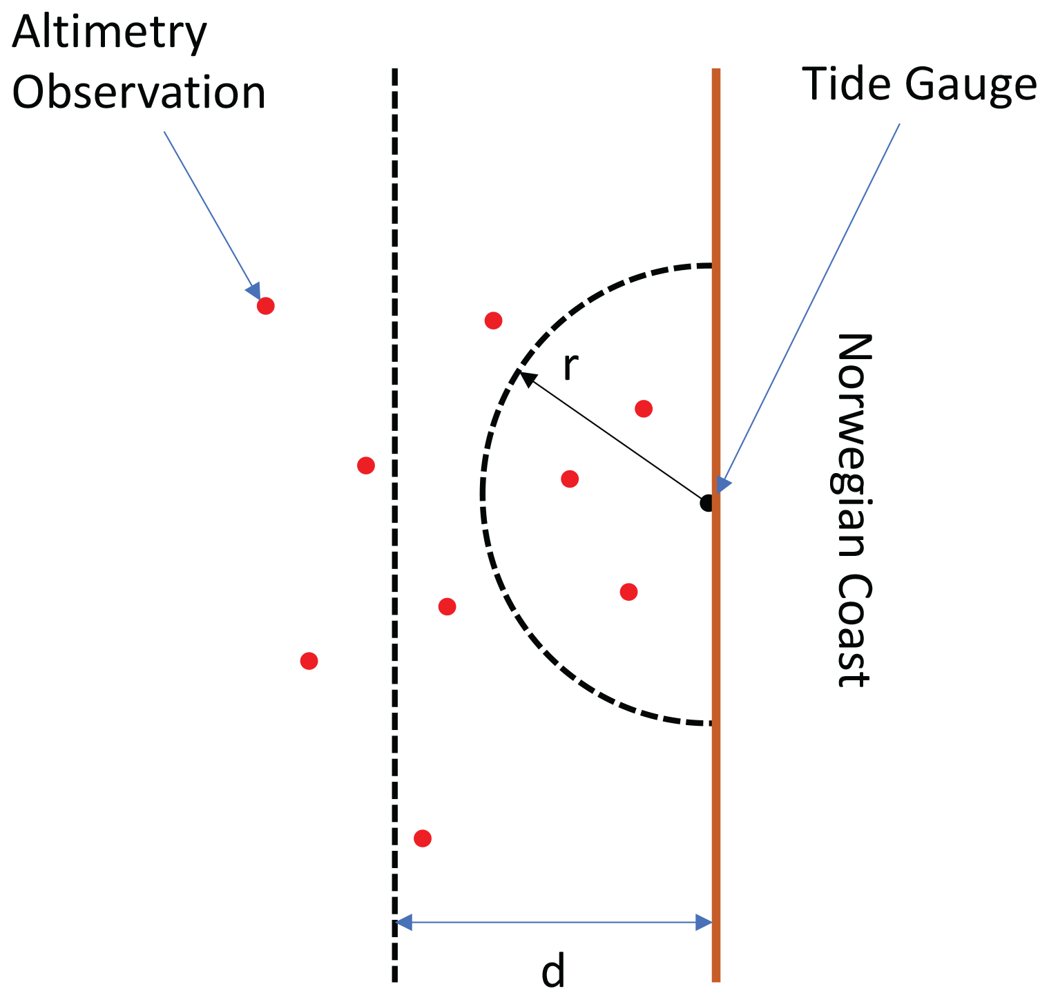
Figure 3 Sketch to illustrate the procedure used to build a monthly averaged SLA time series from the ALES-reprocessed satellite altimetry dataset at each tide-gauge location. The parameter r is the distance from the tide gauge, whereas d is the distance from the coast.

We use the process described above to build a time series of monthly mean sea-level anomaly from altimetry at each tide-gauge location. The resulting sea-level time series have no missing values between Viker and Bodø. Instead, to the north of Bodø, they have 29 missing values which result from the lack of altimetry observations between November 2010 and March 2013.

3.3 Colocation of satellite altimetry and hydrographic stations

We preprocess the altimetry observations to examine the steric contribution to the sea-level variability at each hydrographic station since the two datasets are not colocated in space or in time. More precisely, we select all the altimetry observations located within 20 km from the Norwegian coast and within 200 km from each hydrographic station. Then, for each station, we monthly-average the altimetry observations to build a sea-level anomaly time series from altimetry. The results in the previous subsection give confidence that the monthly mean sea level computed over such a large area is representative of the sea-level variability at each hydrographic station.

3.4 Monthly mean thermosteric, halosteric, and steric sea-level components

To compute the thermosteric and halosteric components of the sea-level variability at each hydrographic station, we first monthly-average the temperature and salinity profiles. Then, at each hydrographic station, we compute the monthly mean thermosteric and halosteric components of the sea level as in Richter et al. (2012):

$$\begin{array}{}\text{(2)}& {\displaystyle }{\mathit{\eta }}_{\mathrm{t}}& {\displaystyle }=\int \mathit{\alpha }(T^{\ast },S^{\ast })\cdot \left(T-T_{\mathrm{0}}\right)\mathrm{d}z,\text{(3)}& {\displaystyle }{\mathit{\eta }}_{\mathrm{s}}& {\displaystyle }=-\int \mathit{\beta }(T^{\ast },S^{\ast })\cdot \left(S-S_{\mathrm{0}}\right)\mathrm{d}z,\end{array}$$

where α and β are the coefficients of thermal expansion and haline contraction, both computed at $T^{\ast }=(T+T_{\mathrm{0}})/\mathrm{2}$ and $S^{\ast }=(S+S_{\mathrm{0}})/\mathrm{2}$. For each hydrographic station, T₀ and S₀ are reference values and represent time-mean temperature and salinity averaged over the entire water column (Siegismund et al., 2007).

The steric component of the sea level at each hydrographic station, η_st, is simply the sum of the corresponding thermosteric and halosteric components of the sea level (Gill and Niiler, 1973).

3.5 Steric contribution to the Norwegian sea level

At each hydrographic station, we assess the contribution of temperature and salinity to the linear trend and the seasonal cycle of the SLA, as well as to the detrended and deseasoned SLA.

We do not use the harmonic analysis approach to estimate the linear trend and the seasonal cycle of the SLA and of the thermosteric, halosteric, and steric components of the sea level at each hydrographic station. Instead, we use simple linear regression to estimate the linear trend, and we compute the monthly climatology of each detrended time series to estimate the corresponding seasonal cycle. Indeed, the seasonal cycle of the SLA and of the thermosteric, halosteric, and steric sea level might depart from the linear combination of the annual and semi-annual cycles.

4 Comparison of satellite altimetry and tide-gauge measurements

In this section, we assess the quality of the ALES-reprocessed coastal altimetry dataset against tide-gauge records by comparing the detrended and deseasoned sea-level variability, the sea-level annual cycle, and sea-level trends provided by the remote sensing and in situ data. We also focus on the stability of linear trend estimates obtained from satellite altimetry (Liebmann et al., 2010; Bonaduce et al., 2016).

4.1 Detrended and deseasoned coastal sea level

Before comparing the detrended and deseasoned SLA from altimetry and tide gauges, we briefly describe how the detrended and deseasoned SLA evolves along the Norwegian coast during the period under study. More precisely, we low-pass-filter the detrended and deseasoned SLAs with a 1-year running mean to identify their main features at each tide-gauge location. Figure 4 shows years when the detrended and deseasoned SLA variations are coherent along the whole Norwegian coast and years when the sea-level variability occurs at smaller spatial scales (between 100 and 1000 km). As an example, between mid-2009 and the beginning of 2011, the detrended and deseasoned SLA shows negative values of up to −6 cm along the entire Norwegian coast. On the contrary, between 2003 and mid-2009, we note a dipole pattern, with SLA with opposite sign in the south and in the north of Norway. Indeed, up to the beginning of circa 2006, the Norwegian coast experienced a negative SLA to the south of Hemsjø and a positive SLA to the north of Heimsjø. During the following 3 years, the opposite situation occurred. These results suggest that, although coherent sea-level variability occurs along the Norwegian coast as seen from tide gauges, there are periods when it does not: during these periods, the sea-level variability is likely driven by local changes.

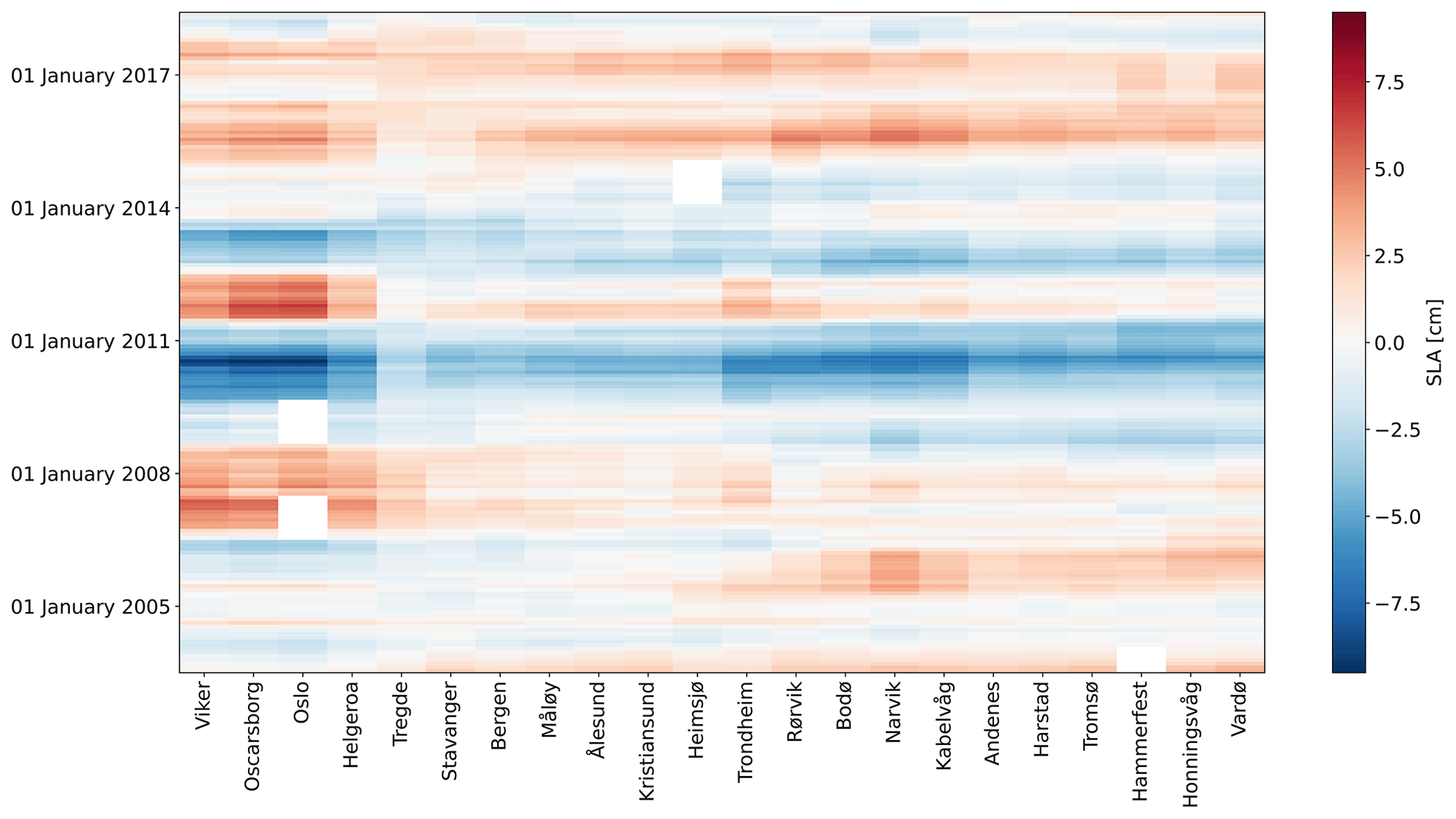
Figure 4 Hovmöller diagram of the detrended and deseasoned monthly mean SLA from tide gauges. The SLA at each tide gauge has been low-pass-filtered with a 1-year running mean. The tide gauges are displayed on the x axis. Time is displayed on the y axis and increases from bottom to top.

Figure 5 shows very good agreement between the detrended and deseasoned monthly mean SLA from ALES and the tide gauges. The two datasets agree best along the west coast of Norway where, if we exclude Trondheim, the linear correlation coefficients exceed 0.90 and the root mean square differences (RMSDs) range between 1.5 and 2.5 cm. As expected, satellite altimetry performs better between Måløy and Rørvik than in southern and northern Norway because of the convergence of altimeter tracks in the region. We suspect that Trondheim is an exception because it is located in the Trondheim fjord, where satellite altimetry might not adequately capture local sea-level variations: the presence of land and patches of calm water affects the quality of the satellite altimetry measurements (Gómez-Enri et al., 2010; Abulaitijiang et al., 2015), and the complex bathymetry and coastline hamper geophysical corrections (Cipollini et al., 2010). Similar peculiarities of the coastline along the Norwegian Trench, in the Skagerrak, and in the Oslofjord are also likely to affect the agreement, causing the linear correlation coefficients to fall between 0.80 and 0.90 and the highest RMSDs to range between 2.5 and 4.5 cm. Instead, in northern Norway, where we find linear correlation coefficients between 0.80 and 0.90 (statistically significant at a 0.05 significance level) and RMSDs between 1.5 and 3 cm, the problem might result from the smaller number of altimetry observations in the region. Indeed, only the tracks of Envisat, SARAL, and SARAL drifting phase cover the Norwegian coast north of 66^∘ N.

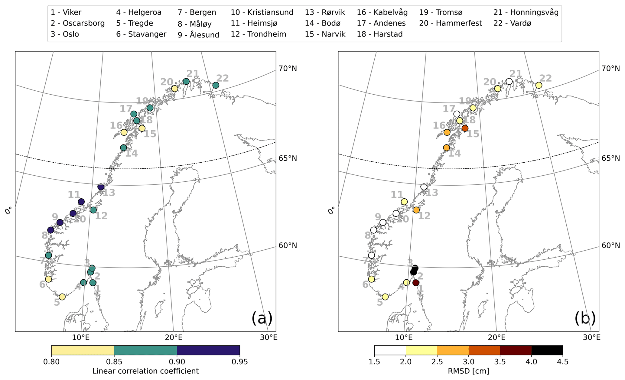
Figure 5 Comparison between coastal sea-level signals from in situ measurements and area-averaged remote sensing data. At each tide-gauge location, the linear correlation coefficient (a) and RMSD (b) between the detrended and deseasoned monthly mean SLA from the ALES altimetry dataset and from the tide gauge. The black dashed line indicates the 66^∘ N parallel.

Figure 6 supports our previous conclusions on the relationship between satellite altimetry and the tide gauges at Trondheim, Oslo, and Oscarborg. In Fig. 6, we show, for each tide gauge, the standard deviation of the linear correlation coefficient and of the RMSDs over all the possible combinations of the distance from the coast and from the tide gauge to measure the geometrical uncertainty of the SLA estimates from satellite altimetry. We find that, at Trondheim, both the linear correlation coefficient and the RMSD depend more on the size of the selection window when compared to other regions of the Norwegian coast. Similarly, at Oslo and Oscarborg, we note an anomalously high standard deviation of the linear correlation coefficient. We expect anomalously high values of the standard deviation of the linear correlation coefficients and RMSDs because these three tide gauges are in sheltered areas (Trondheim is in the Trondheim fjord, whereas Oslo and Oscarborg are in the Oslofjord), which can favour the formation of patches of calm water and negatively affect the quality of the satellite altimetry observations.

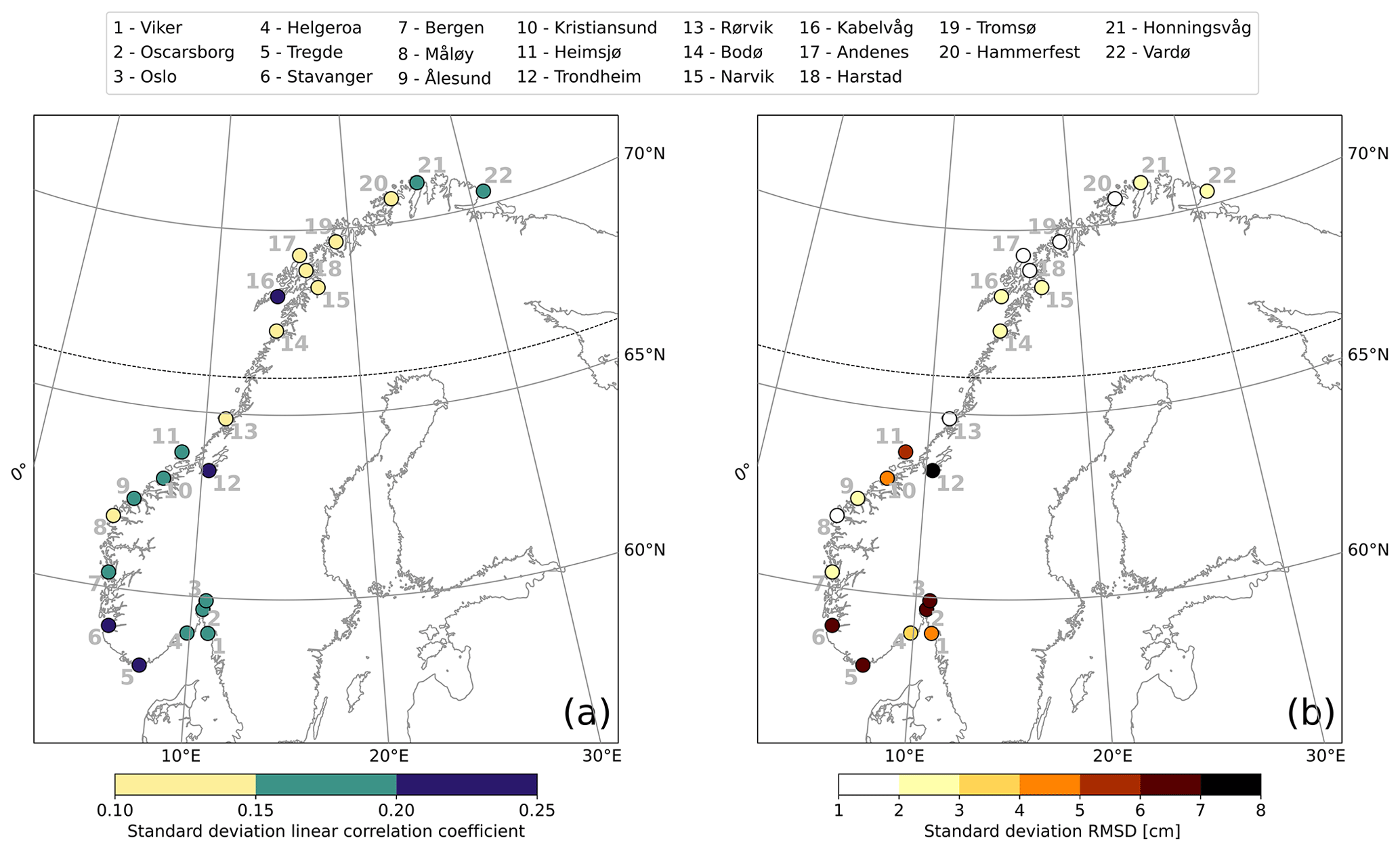
Figure 6 Comparison between coastal sea-level signals from in situ measurements and area-averaged remote sensing data. At each tide-gauge location, the standard deviation of the linear correlation coefficients (a) and of the RMSDs (b) is computed over each possible combination of the distance from the coast and of the distance from the tide gauge. The black dashed line indicates the 66^∘ N parallel.

4.2 Annual cycle of coastal sea level

Figures 7 and 8 show good agreement between the annual cycle estimated using the ALES altimetry dataset and the tide gauges. The difference between the amplitudes of the annual cycle from ALES and the tide gauges ranges between −1.2 and 1.8 cm. However, at most tide-gauge locations (15 out of 22), the differences are much smaller at between −1 and 1 cm, which is less than 10 % of the amplitude of the corresponding annual cycle (Fig. 7a). We note that the differences between the amplitudes are mostly negative along the southern and western coast of Norway and that, to the north of Rørvik, they become smaller and even change sign at some locations (Fig. 7b).

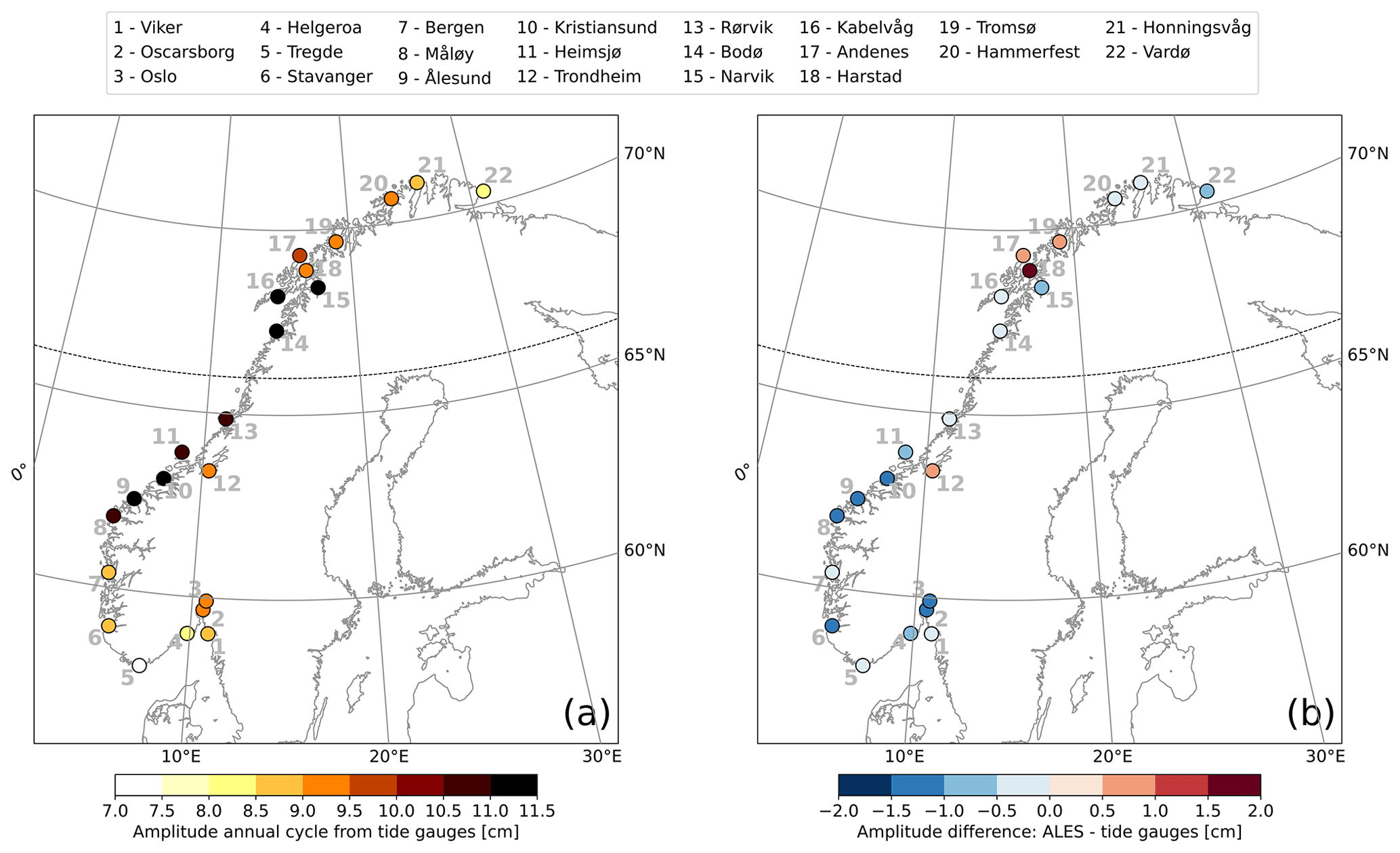
Figure 7 Comparison between the amplitude of coastal sea-level annual cycle from in situ measurements and area-averaged remote sensing data. At each tide-gauge location, the amplitude of the annual cycle from the tide gauges (a) and difference between the amplitude of the annual cycle from the ALES-reprocessed altimetry dataset and the tide gauges (b). The black dashed line indicates the 66^∘ N parallel.

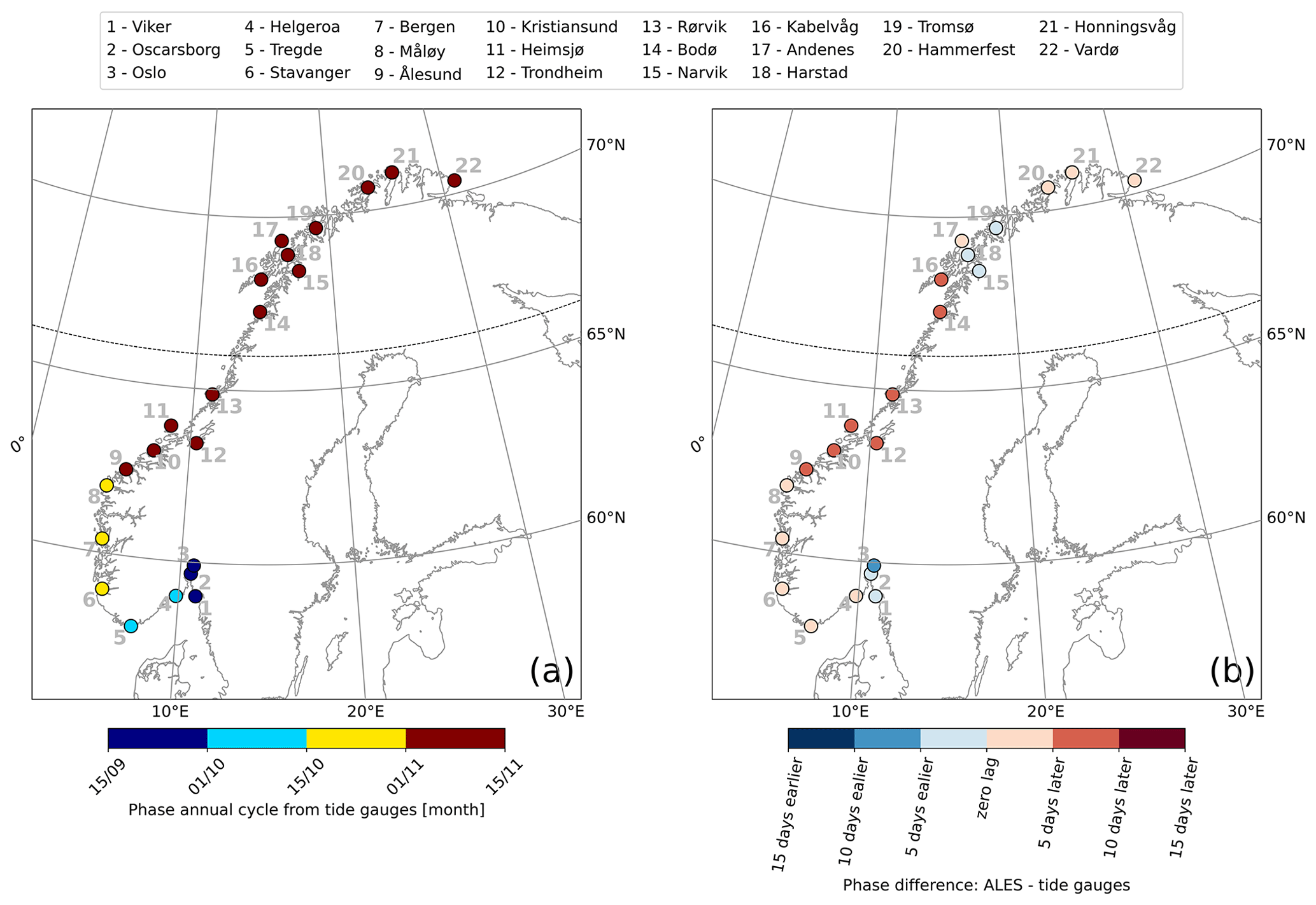
Figure 8 Comparison between the phase of coastal sea-level annual cycle from in situ measurements and area-averaged remote sensing data. At each tide-gauge location, the phase of the annual cycle from the tide gauges (a) and phase difference of the annual cycle from the ALES-reprocessed altimetry dataset and from the tide gauges (b). The black dashed line indicates the 66^∘ N parallel.

The difference between the phases of the annual cycle estimated using the ALES altimetry dataset and the tide gauges ranges between −10 and +10 d (Fig. 8b). Such a great similarity indicates that both radar altimetry and the tide gauges capture the phase lag of approximately 2 months between the annual cycle in the north and in the south of Norway. The annual cycle peaks during the second half of September in the Skagerrak and in the Oslofjord region, in October along the Norwegian Trench and in southwestern Norway, and mainly during the first week of November north of Kristiansund.

4.3 Linear trend of coastal sea level

The differences between sea-level trend estimates obtained from the in situ and remotely sensed signals range between −0.85 and 1.15 mm yr⁻¹ along the Norwegian coast (Fig. 9). Both datasets return a similar spatial dependence of the sea-level trend along the Norwegian coast, with the lowest values found in the Skagerrak and the Oslofjord (between 2 and 3 mm yr⁻¹) and the highest to the north of Heimsjø (around 4 mm yr⁻¹). Moreover, the two datasets return a similar uncertainty of the sea-level trend at each tide-gauge location.

Figure 9 At each tide-gauge location, the linear trend of the SLA from the ALES-reprocessed altimetry dataset (black dots) and from tide gauges (red dots). The error bars show the 95th confidence intervals of the sea-level trend at each tide-gauge location.

Despite their similarities, we still find that the difference between the sea-level trend from altimetry and tide gauges is significantly different from zero at a 0.05 significance level at 3 out of 22 tide gauges. Following Benveniste et al. (2020), we assess the significance in terms of fractional differences (FDs). Fractional differences are defined as $\text{FD}=\left|\mathit{\tau }\right|/(t_{\mathrm{0.05}/\mathrm{2}}\cdot \text{SE}\cdot N/N^{\ast })$, where $\left|\mathit{\tau }\right|$ is the absolute value of the linear trend of the SLA difference between altimetry and each tide gauge, $t_{\mathrm{0.05}/\mathrm{2}}$ is the critical value of the Student's t test distribution for a 95 % confidence level with $N^{\ast }-\mathrm{2}$ degrees of freedom, SE is the standard error, and $N/N^{\ast }$ is the ratio between the total number of observations and the effective number of degrees of freedom. When FD>1, the difference between the two trends is statistically significant at a 0.05 significance level, a condition that occurs at Tregde, Måløy, and Bergen. Interestingly, none of these tide gauges are located north of 66^∘ N despite only some of the altimetry missions considered in this study having an inclination exceeding 66^∘ N (namely, Envisat, SARAL, SARAL drifting phase). Therefore, the fewer altimetry observations to the north of 66^∘ N seem not to deteriorate the agreement between the ALES-reprocessed altimetry and the tide gauges.

Following Liebmann et al. (2010), we use the satellite altimetry data to assess how strongly the sea-level trend depends on the time length of the period considered. Each point in Fig. 10 shows the sea-level trend computed over the number of years on the y axis up to the year specified on the x axis. Between 2003 and circa 2013, we do not find a significant sea-level trend along the Norwegian coast. Indeed, with very few exceptions, the trends are not statistically different from zero at a 0.05 significance level. The exceptions consist of a small number of cases, each characterized by a sea-level trend lower than −4 mm yr⁻¹.

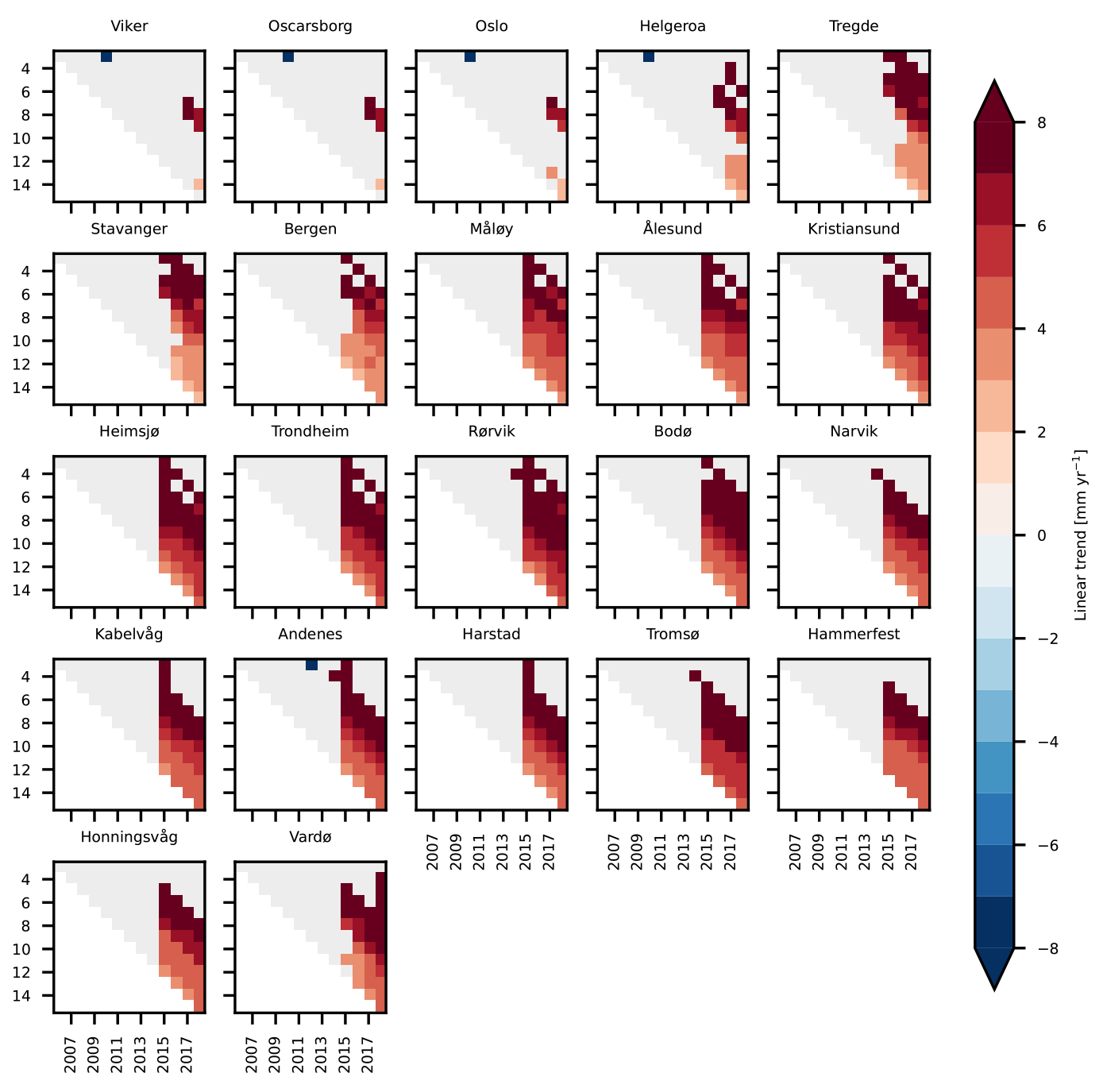
Figure 10 Stability of the sea-level trend along the Norwegian coast. At each tide-gauge location, the linear trend of the SLA from ALES as a function of the period considered. Each panel refers to a tide-gauge location and shows all the possible trends computed up to the year shown on the x axis, considering the number of years displayed on the y axis. For example, the point (x=2014, y=5) in each panel shows the linear trend of the SLA computed over the 5-year period between 1 January 2009 and 31 December 2014. Light gray is used to mask values that are not significantly different from zero at the 0.05 significance level.

On the contrary, with the exception of the three southernmost tide-gauge locations, we note a significant positive sea-level trend along the entire coast of Norway when the period considered for the calculation ends in 2015 or later. The linear trends decrease as the length of the period selected increases. When sea-level rates are computed over periods of a few years only, they even exceed 6 mm yr⁻¹. Instead, over longer periods of time (e.g. more than 10 years), they mainly range between 3 and 5 mm yr⁻¹. A visual inspection of the time series confirms that the sea level has increased since 2014.

5 Steric contribution to the sea-level variability

In this section, we use the Norwegian set of hydrographic stations to assess how temperature and salinity affect the sea-level trend, the seasonal cycle of sea level, and the detrended, deseasoned sea-level variability at different locations along the Norwegian coast.

5.1 Variability of the thermosteric and the halosteric sea-level components

The variability of the thermosteric and halosteric sea-level components along the Norwegian coast mainly occurs over two different spatial and temporal scales (Fig. 11). Notably, the seasonal cycle dominates the thermosteric sea-level variability at each hydrographic station and is responsible for the thermosteric sea level varying approximately uniformly along the coast of Norway. On the contrary, the halosteric component shows a variability at shorter spatial and temporal scales, possibly due to the contributions from local rivers. The main exceptions are, due to their proximity, the two sets of twin hydrographic stations, Indre Utsira–Ytre Utsira and Eggum–Skrova (Fig. 1).

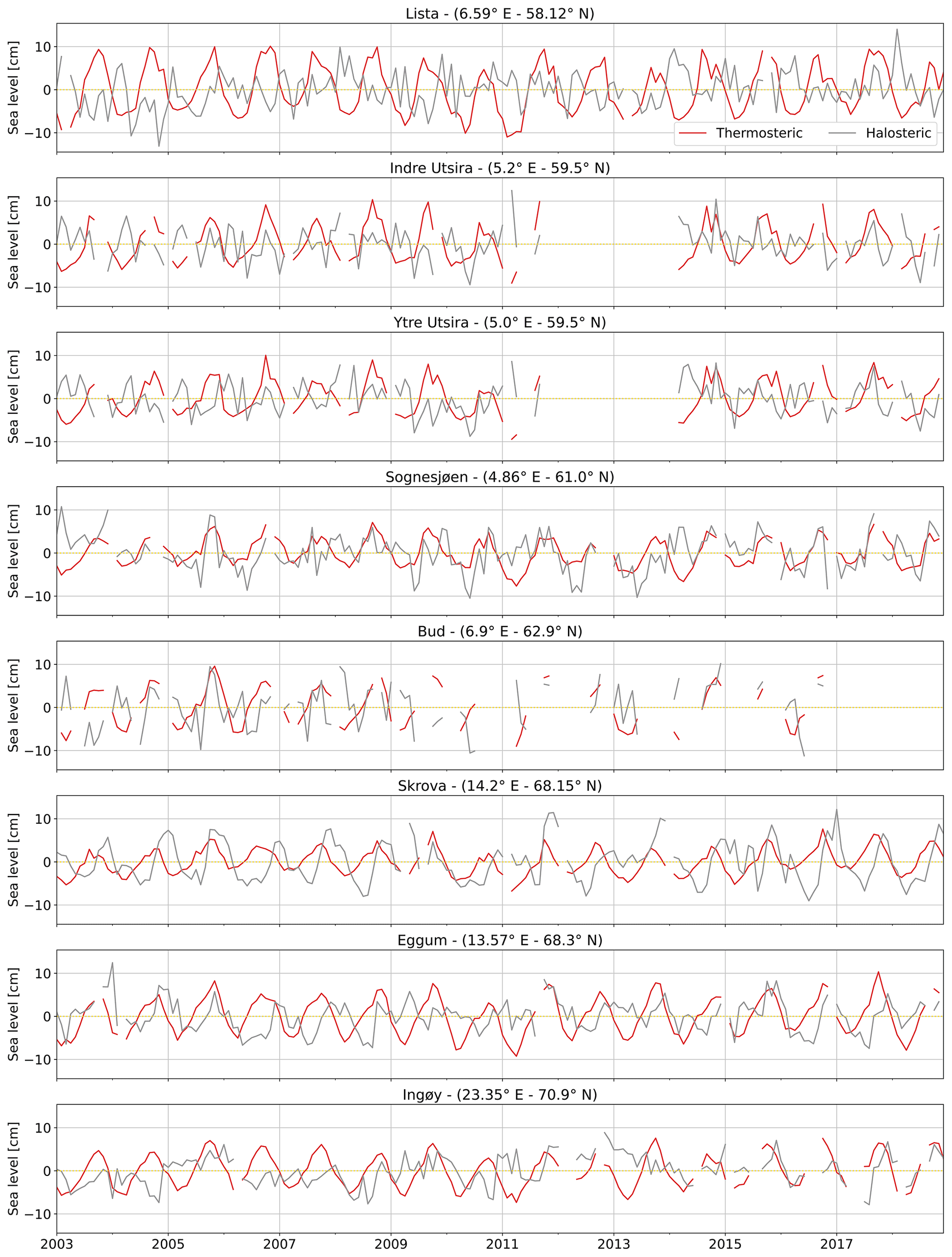
Figure 11 Thermosteric (red) and halosteric (gray) components of the sea-level anomaly at each hydrographic station along the Norwegian coast.

Despite these differences, both the thermosteric and halosteric components of the sea level give a comparable contribution to the sea-level variability along the Norwegian coast (Fig. 11). This ranges approximately between −10 and 10 cm at each hydrographic station.

In the following sections, we investigate the spatial variability of these two components along the Norwegian coast, focusing on the linear trend, the seasonal cycle, and the residuals, as well as on their contribution to the sea-level variability in the region.

5.2 Steric contribution to the sea-level trend

In this section, we perform a fit-for-purpose assessment of the Norwegian hydrographic station network to obtain estimates of the steric sea-level trends from satellite altimetry and in situ data.

Over the period 2003–2018, we find that the linear trends of the thermosteric, halosteric, and steric components of the sea level approximately range between −1.0 and 2.5 mm yr⁻¹. The steric contributions to coastal sea-level trends experience large spatial variability that is even negative at Sognesjøen and reaches a peak of approximately 55 % of the sea-level trend estimated from satellite altimetry at Lista and Ingøy. Moreover, when we compare the thermosteric and halosteric signals at these locations, we note that the latter contributes more than the former to the coastal sea-level trends (up to 50 % of the sea-level trend from altimetry). The width of the confidence intervals of the thermosteric, halosteric, and steric contributions ranges between 4.0 and circa 12.0 mm yr⁻¹, with northern Norway exhibiting larger uncertainties (Fig. 12). This is a result of the high inter-annual variability of the thermosteric and halosteric components in the region (Figs. B1 and B2), which leads to fewer effective degrees of freedom and, therefore, to less accurate estimates of the linear trend.

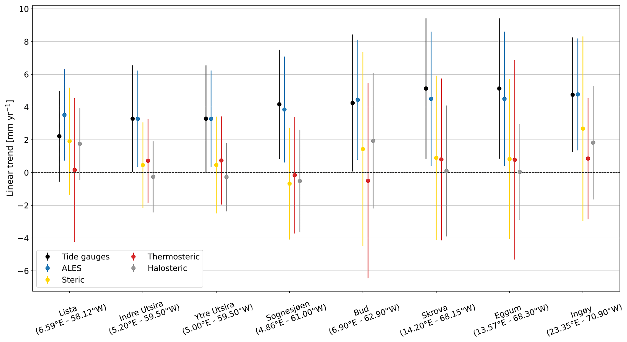
Figure 12 At each hydrographic station, the linear trend of the sea level from tide gauges and from ALES (black and blue dots, respectively), as well as of the steric, thermosteric, and halosteric components of the sea level (yellow, red, and gray dots, respectively). The bars indicate the 95 % confidence intervals.

We also test if using tide gauges, instead of satellite altimetry, could alter our estimates of the relative contribution of these components (thermosteric, halosteric, and steric) to the sea-level trend along the coast of Norway. Such alteration may indeed occur because the sea-level variations measured by the Norwegian tide gauges might not properly represent those occurring in proximity to the hydrographic stations since the two sets of instruments are not colocated in space (Fig. 1).

With the exception of Lista, the choice of the dataset has a minimal influence on the estimates of the thermosteric, halosteric, and steric relative contributions to the sea-level trend along the coast of Norway. We reach this conclusion by visual inspection, but we also provide a more quantitative analysis based on the ratio between the linear trend of the SLA and of the thermosteric, halosteric, and steric components of the sea level. We find that, apart from Lista, the choice of the dataset modifies such a ratio by less than 13 %. At Lista, the change amounts to 59 % and results from the ALES-retracked satellite altimetry dataset returning a sea-level trend approximately 1.6 times larger than that provided by the tide gauge at Tregde (this is the tide gauge we use to compute the thermohaline contribution at Lista). Such a large variation is expected since, as we have already noticed, the sea-level rates obtained considering tide-gauge and satellite data at Tregde show less accurate agreement (Figs. 9 and C5).

5.3 Steric contribution to the seasonal cycle of sea level

In this section, we build on the results by Richter et al. (2012) and assess the thermosteric, halosteric, and steric contributions to the seasonal cycle of the sea level at each hydrographic station along the Norwegian coast.

We find that using the tide-gauge data, instead of satellite altimetry measurements, only minimally affects the estimate of the thermosteric, halosteric, and steric contributions to the seasonal cycle of SLA (Fig. 13), even though the tide gauges are not colocated in space with the hydrographic stations. Indeed, the seasonal cycle returned by satellite altimetry at each hydrographic station strongly resembles that returned by the nearby tide gauge (Fig. 13, fourth column). At the same time, the RMSD between the seasonal cycle of the SLA and steric sea level, scaled by the range (maximum minus minimum) of the seasonal cycle of SLA, minimally depends on the dataset used (Table 1, first and second columns).

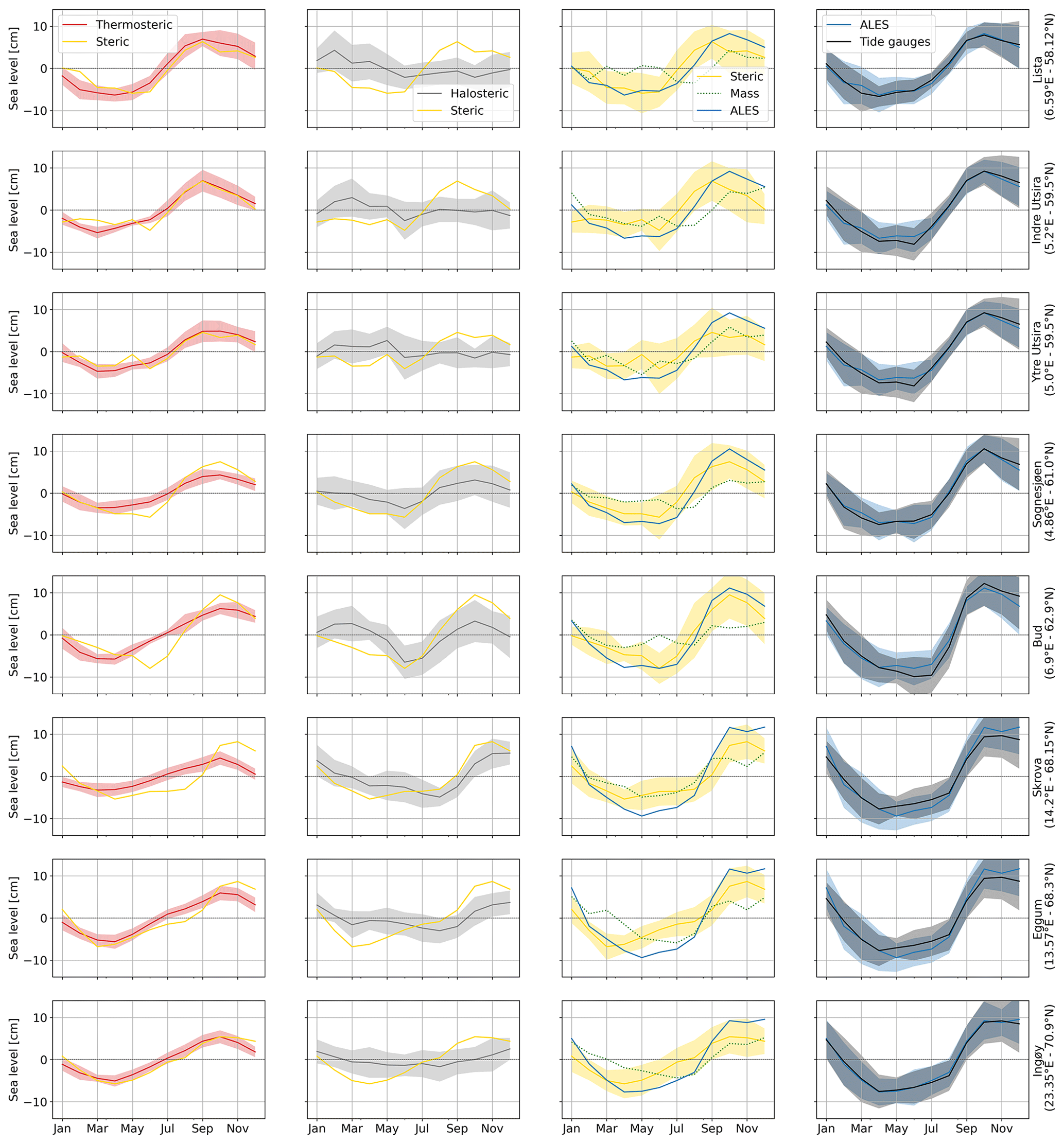
Figure 13 Monthly climatology of the sea-level signals at the hydrographic station positions. The panels show the steric (yellow lines), thermosteric (red lines), halosteric (gray lines), and mass (green lines) components of the sea level. The monthly climatology obtained from altimetry (blue lines) and tide-gauge (black lines) measurements is also shown. The shading enveloping the monthly climatologies shows the region departing from each line by 1 climatological standard deviation.

Table 1 Comparison between the seasonal cycle of SLA from ALES, of SLA from the tide gauges, and of steric sea level at each hydrographic station position. The first and the second columns show, for ALES and the tide gauges, the RMSD between the seasonal cycle of SLA and the steric sea level scaled by the range (maximum minus minimum) of the seasonal cycle of SLA. The third and the fourth columns show the ratio of the ranges and the lag of maximum correlation of the seasonal cycle of SLA from ALES and steric sea level.

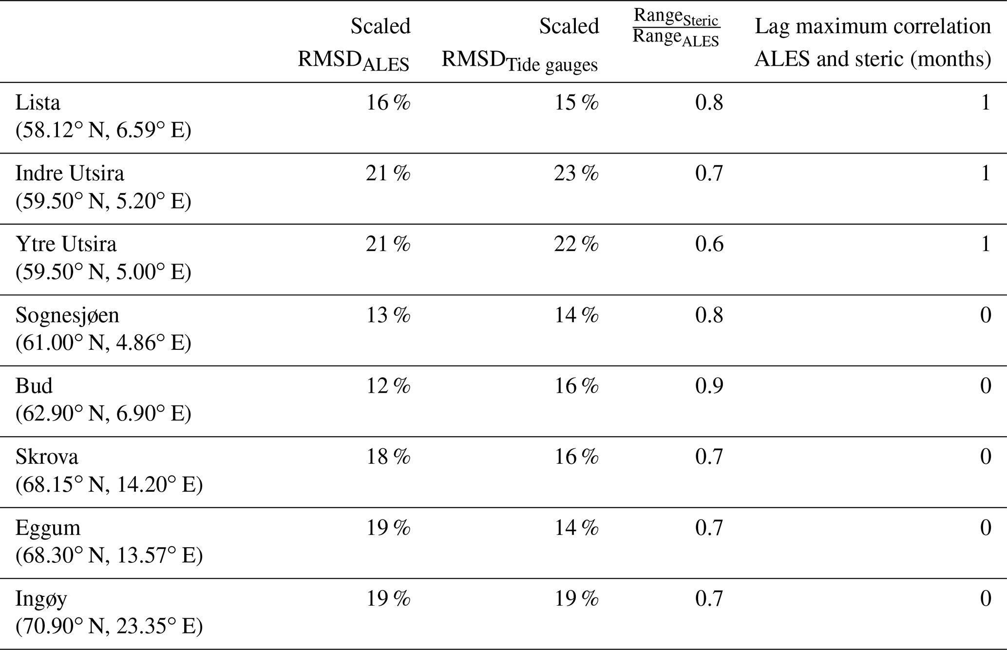
We also note that density changes substantially contribute to the seasonal cycle of SLA along the Norwegian coast, as shown by Fig. 13 and Table 1. The seasonal cycle of SLA and steric sea level are 1 month out of phase along the southern and western coast of Norway up to Yndre Utsira and in phase over the remaining part of the Norwegian coast. Moreover, the ratio between the range of seasonal cycles of steric sea level and of SLA varies between 0.6 at Ytre Utsira and 0.9 at Bud (Table 1, third column).

Along the Norwegian coast, the seasonal cycle of steric sea level is more affected by variations in temperature than in salinity. We note that, with the exception of Bud and Skrova, the seasonal cycle of the steric component mostly resembles that of the thermosteric component in terms of both amplitude and phase. At the same time, we note a clear discrepancy between the seasonal cycle of the halosteric and steric components in both southern Norway, where they are in anti-phase, and at Bud, where the seasonal cycle of the halosteric sea level is dominated by the semi-annual cycle. A more quantitative analysis returns comparable results; the RMSD between the steric and halosteric seasonal cycles exceeds by a factor of 1.4 the RMSD between the steric and thermosteric seasonal cycles along the entire coast of Norway (with the exception of Skrova, where the ratio between the two RMSDs is 0.7).

5.4 Detrended and deseasoned coastal sea level and its components

The detrended and deseasoned thermosteric sea level along the Norwegian coast shows larger spatial variability compared to the detrended and deseasoned halosteric component (Fig. 14). The correlation matrix of the thermosteric sea level (Fig. 14a) shows larger values compared to the one obtained considering the halosteric sea-level signals (Fig. 14b). As an example, while the minimum linear correlation coefficient between two adjacent hydrographic stations in Fig. 14a is 0.52, it is only 0.19 in Fig. 14b. We briefly discuss the small spatial-scale variability of the halosteric sea level along the Norwegian coast in the “Discussion and conclusions” section of the paper.

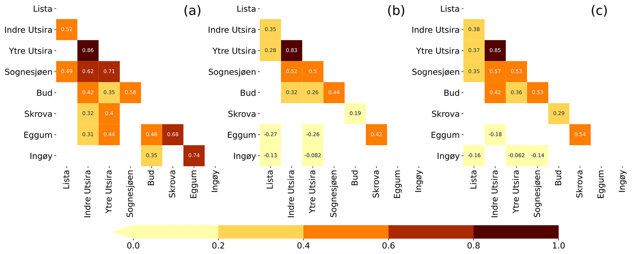
Figure 14 Correlation matrices of the detrended and deseasoned thermosteric (a), halosteric (b), and steric (c) components of the sea level at each hydrographic station. Correlation values that are not significant at a 0.05 significance level have been omitted.

From Fig. 14c, we also note that the values of the correlation matrix of the steric sea level fall between those of the thermosteric and halosteric components. This suggests that the thermosteric and halosteric components of the sea level give a similar contribution to the sea-level variability along the Norwegian coast.

6 Discussion and conclusions

In this paper, we have first assessed the ability of the ALES-reprocessed satellite altimetry dataset to capture the Norwegian sea-level variability over a range of timescales. Then, we have used data from hydrographic stations to quantify the steric contributions to the sea-level variability along the coast of Norway.

Along the Norwegian coast, the sea-level trend from the ALES-reprocessed satellite altimetry dataset is found to be compatible with the estimates from tide gauges. Their difference only ranges between −0.85 and 1.15 mm yr⁻¹ and is significantly different from zero at the 95 % confidence level at 19 out of 22 tide-gauge locations. Because of this good agreement, the choice of the sea-level dataset (either tide gauges or ALES) has a minimal impact on the estimates of the thermosteric, halosteric, and steric relative contributions to the sea-level trend. Despite the large uncertainties, this result is encouraging since it suggests that the ALES dataset can be used to partition the sea-level variability in regions of the coastal ocean not covered by tide gauges. At the same time, it confirms the validity of previous sea-level studies in the region which only used tide-gauge data (e.g. Richter et al., 2012).

Regarding the comparison between the ALES-retracked and the along-track (L3) conventional altimetry datasets, we find that the former shows, on average, a 6 % improvement, despite it being well within the margins of error. This improvement is most evident at Bodø, Kabelvåg, and Tromsø in northern Norway, where the agreement with the tide gauges improves by 19 %, 23 %, and 24 %, respectively. The use of the ALES retracker for more satellite altimetry missions, in order to have more observations and to cover the period before July 2002, might help reduce the uncertainties and return a more statistically significant result.

A comparison with Breili et al. (2017), wherein an along-track (L3), multi-mission conventional altimetry dataset was used to analyse the sea-level trend along the Norwegian coast, returns comparable results. We cannot, however, directly compare the linear trends in this work with those in Breili et al. (2017) since they focus on a different period (1993–2016), and the sea-level trend along the Norwegian coast strongly depends on the length of the time window considered (Fig. 10). However, when assessing how the conventional satellite altimetry datasets compare with tide-gauge records in terms of the linear trend computed over a common time window, ALES again shows an improvement in northern Norway between Bodø and Tromsø, where the difference between the linear trend from ALES and the tide gauges is small (up to 0.5 mm yr⁻¹) compared to circa 1 to 3 mm yr⁻¹ found by Breili et al. (2017) using a conventional altimetry dataset.

The ALES-retracked satellite altimetry dataset is found to underestimate the amplitude of the annual cycle along large portions of the Norwegian coast (Fig. 7). Even though the difference between the two sets of estimates is not significant at a 95 % significance level (the 95 % confidence interval is approximately twice the standard error), we find this result interesting because of its consistency. We do not expect such a consistency to depend on the ALES retracker since we find a comparable result when we use the along-track (L3) conventional altimetry product (Fig. C3). We rather suspect a dependence of the amplitude of the annual cycle on the bathymetry and, therefore, on the distance from the coast, as shown by Passaro et al. (2015) along the Norwegian sector of the Skagerrak.

A comparison with Volkov and Pujol (2012) shows that the ALES-retracked satellite altimetry better captures the sea-level annual cycle along the coast of Norway with respect to the gridded sea-level altimetry products. In that study, the authors considered six tide gauges along the Norwegian coast, namely Kristiansund, Rørvik, Andenes, Hammerfest, Honningsvåg, and Vardø, to assess the quality of satellite altimetry maps at the northern high latitudes. Except for Andenes, we note that the ALES-reprocessed coastal altimetry dataset allows for more accurate estimates of the sea-level annual cycle, reducing the differences with the in situ sea-level records by a factor of 3 to 6 compared to gridded satellite altimetry products.

We also assess the steric contribution to the seasonal cycle of SLA. Our results show that the steric variations and, in particular, the thermosteric variations considerably contribute to the seasonal cycle of the sea level along the entire Norwegian coast. Moreover, we find that the relative contributions of the thermosteric, halosteric, and steric sea level minimally depend on whether we use tide gauges or satellite altimetry. This is indicative of the large-scale spatial pattern associated with the seasonal cycle of SLA.

The detrended and deseasoned sea-level variability along the Norwegian shelf resembles the along-slope wind index proposed by Chafik et al. (2019). We note that the similarities between the two are stronger along the western and northern coast of Norway than in the south. Indeed, from Oslo to Ålesund, SLA signals depart from the along-slope wind index between 2003 and 2008, probably due to local effects, such as the Baltic outflow. We refer to local effects since Chafik et al. (2019) attributed the inter-annual sea-level variability over the northern European continental shelf to the along-slope winds, which might regulate the exchange of water between the open ocean and the shelf through Ekman transport.

Because the detrended and deseasoned SLA pattern is coherent over large distances along the Norwegian coast (see also Chafik et al., 2017), coastal altimetry observations located a few hundred kilometres apart can be representative of the sea-level variations occurring at a particular tide-gauge location. This explains why we can average the SLA from altimetry over an area a few hundred kilometres wide around each tide-gauge location to maximize the linear correlation coefficient between the detrended and deseasoned SLA from satellite altimetry and the tide gauges (Sect. 3.2). Moreover, it also partly explains the good agreement between satellite altimetry and tide gauges since, as we average over a large number of satellite altimetry observations, we increase the temporal sampling provided by altimetry, and therefore we reduce the noise in the resulting SLA (Oelsmann et al., 2021).

The small-scale variability of the detrended and deseasoned sea-level halosteric component (Fig. 14) does not reconcile with the good agreement between tide-gauge sea-level signals and the ALES-reprocessed altimetry dataset. Indeed, to compare the two datasets, we have averaged the satellite altimetry observations over an area a few hundred kilometres wide around each tide gauge. However, Fig. 14 suggests that the estimates of the halosteric component can change significantly over an area of this size. Furthermore, while this component has a magnitude comparable to that of the detrended, deseasoned SLA (not shown), it only explains a small fraction (from 3 % to 11 %) of the difference between the sea-level signals from altimetry and the tide gauges.

Future work is thus warranted to understand whether the small-scale variability of the halosteric component of the sea level along the Norwegian coast results from measurement issues. For example, ocean salinity is measured approximately once a week at Skrova and approximately twice a month at the remaining hydrographic stations: this aliases the sub-weekly salinity variations into the lower-frequency components and, consequently, might significantly alter the monthly mean salinity values. A new study, which takes benefit from ships of opportunity as well as synergies between different observational platforms and ocean models, could help clarify this issue.

To conclude, we have demonstrated the advantage of the ALES retracker over the conventional open-ocean retracker along the coast of Norway. The retracking of earlier altimeter missions would, however, be necessary to provide a more accurate estimate of the sea-level variability along the coast of Norway and could possibly be used to understand whether the sea-level rise in the region is accelerating. Still, this paper gives confidence that the ALES-reprocessed altimetry dataset can be fruitfully used to measure coastal sea-level variations in regions poorly covered by tide gauges.

Appendix A

To estimate the uncertainty associated with the sea-level trends derived from tide gauges and the ALES-retracked satellite altimetry dataset (Fig. 9), we need to account for the effective degrees of freedom in the sea-level anomaly time series. Indeed, successive points in the SLA time series might be correlated and, therefore, not drawn from a random sample.

To determine the effective number of degrees of freedom, we produce semi-variograms of the detrended and deseasoned SLA from the tide gauges and the altimetry dataset. The semi-variogram is defined as

$$\begin{array}{}\text{(A1)}& \mathit{\gamma }\left(t\right)={\displaystyle \frac{\mathrm{1}}{\mathrm{2}}}\cdot \text{var}\left[x\right(t)-x(t+\mathit{\tau }\left)\right],\end{array}$$

where x(t) is the time series under study, var stands for variance, and τ is the time lag.

The number of degrees of freedom is obtained by fitting the semi-variograms with a spherical function of the form

$$\begin{array}{}\text{(A2)}& \left\{\begin{array}{ll}c\left(h\right)=b+C_{\mathrm{0}}\cdot \left(\mathrm{1}-\frac{\mathrm{3}}{\mathrm{2}}\frac{\left|h\right|}{a}+\frac{\mathrm{1}}{\mathrm{2}}\frac{|h{|}^{\mathrm{3}}}{a^{\mathrm{3}}}\right)& \text{if }h\le a\\ c\left(h\right)=b+C_{\mathrm{0}}& \text{if }h>a,\end{array}\right.\end{array}$$

where h is the fitting parameter, and a is the effective range or, in other words, the lag needed for the semi-variogram to reach a constant value. Semi-variograms are preferred to autocorrelations in geostatistics because they better detect the non-stationarity of time series.

We use the fit to determine the lag at which each semi-variogram reaches a plateau, since it indicates the decorrelation timescale of the time series. The effective number of degrees of freedom corresponds to the ratio between the length of the time series and the lag.

We find that the lag only minimally depends on the tide-gauge location and on whether we consider the detrended and deseasoned SLA from the altimetry dataset or the tide gauges (Figs. A1 and A2). The semi-variograms obtained from both altimetry and the tide gauges return a lag of 2 months at each tide-gauge location, with the exception of three stations in southern Norway (Viker, Oscarborg, and Helgeroa), where the SLA from the tide gauges is characterized by a 3-month lag.

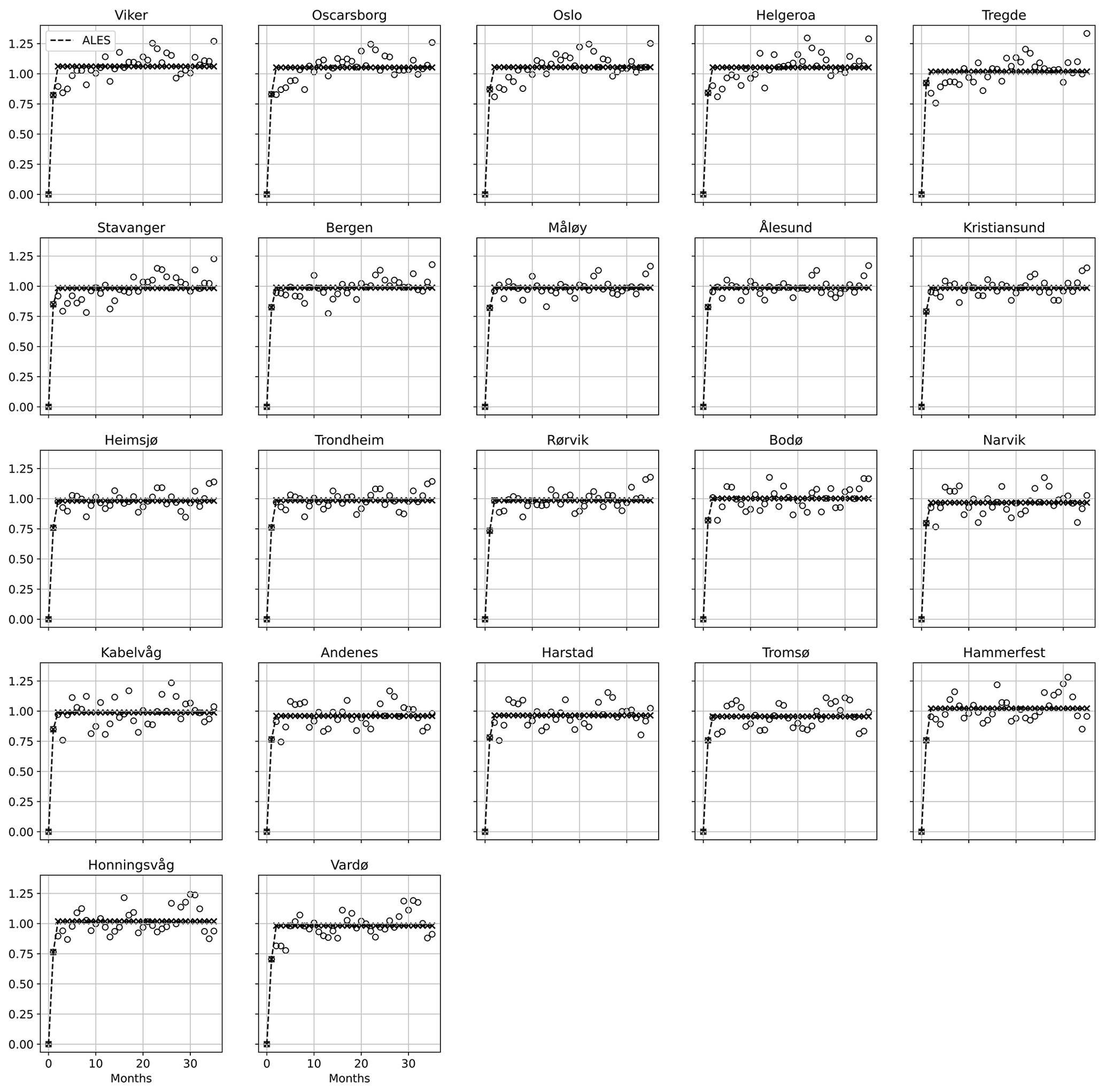
Figure A1 For each tide gauge along the Norwegian coast, semi-variogram of the detrended and deseasoned SLA estimated from the ALES-retracked satellite altimetry (empty circles) and corresponding fit (crosses connected by a dashed line). At each tide-gauge location, we scaled each semi-variogram by the variance of the corresponding detrended and deseasoned SLA for all the plots to have the same limits on the y axis.

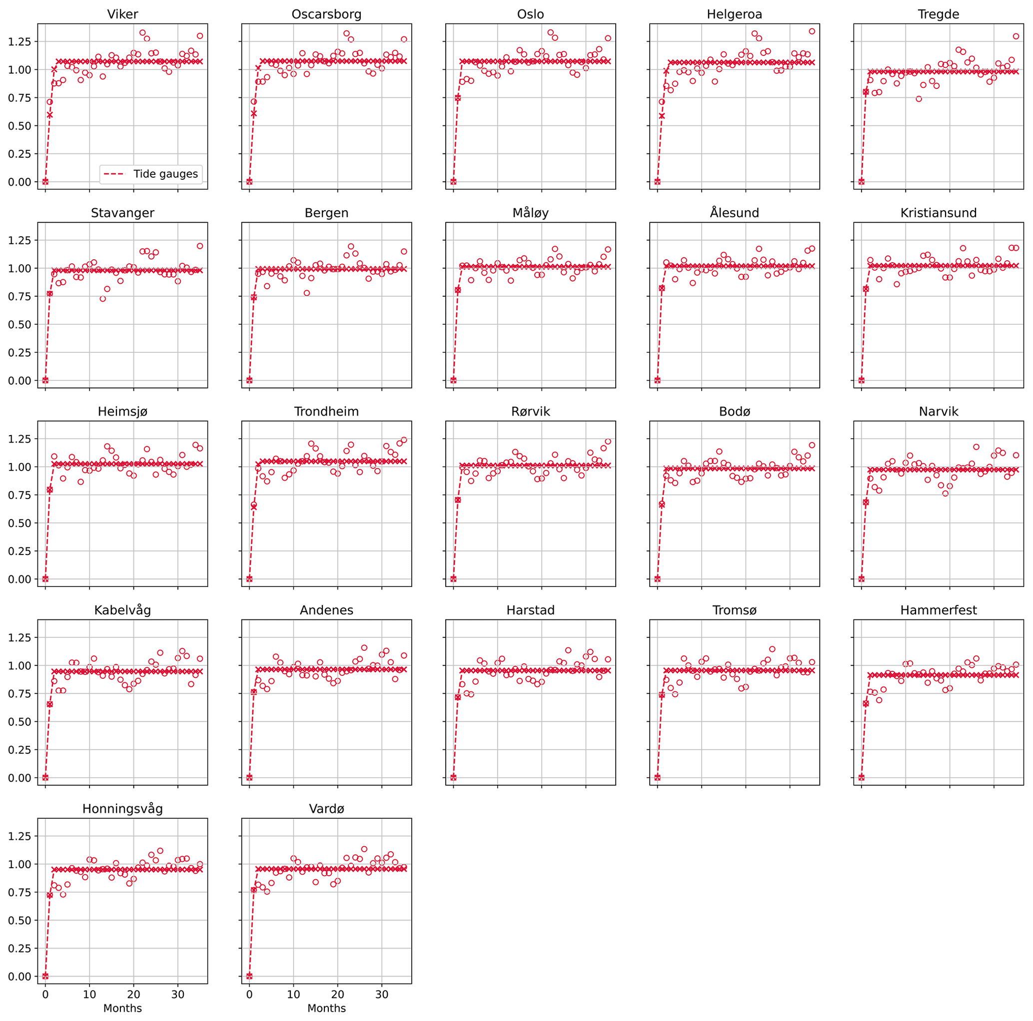
Figure A2 For each tide gauge along the Norwegian coast, semi-variogram of the detrended and deseasoned SLA measured by the tide gauge (empty circles) and corresponding fit (crosses connected by a dashed line). At each tide-gauge location, we scaled each semi-variogram by the variance of the corresponding detrended and deseasoned SLA for all the plots to have the same limits on the y axis.

We use the same approach to compute the uncertainty associated with the linear trend of the difference between the SLA from satellite altimetry and the tide gauges, with only one exception. We noticed that the spheric model does not fit the semi-variogram for Trondheim. Therefore, for Trondheim, we opted for an exponential model:

$$\begin{array}{}\text{(A3)}& \mathit{\gamma }\left(t\right)=b+C_{\mathrm{0}}\left(\mathrm{1}-e^{-\frac{h}{a}}\right),\end{array}$$

where h is the fitting parameter, and a is the range parameter. An exponential function is preferred over the spherical function when the time series shows a strong temporal correlation.

The serial correlation is negligible along the entire Norwegian coast with the exception of Viker, Oscarborg, Oslo, and Narvik, where the semi-variograms return a 2-month lag (Fig. A3). At Trondheim, instead, we find a much larger lag (approximately 10 months).

We use the effective number of degrees of freedom when we compute the confidence intervals of the sea-level rates in Fig. 9. We compute the 95 % confidence interval of the linear trend as follows:

$$\begin{array}{}\text{(A4)}& \text{CI}=t_{\mathrm{0.05}/\mathrm{2},N^{\ast }-\mathrm{6}}\cdot \sqrt{{\displaystyle \frac{N-\mathrm{1}}{N^{\ast }-\mathrm{1}}}}\cdot \text{SE},\end{array}$$

where SE is the standard error of the linear trend computed as if $N^{\ast }=N$ (the total number of observations in the time series), and $t_{\mathrm{0.05}/\mathrm{2},N^{\ast }-\mathrm{6}}$ represents the t values computed using $N^{\ast }-\mathrm{6}$ degrees of freedom at a 0.05 significance level.

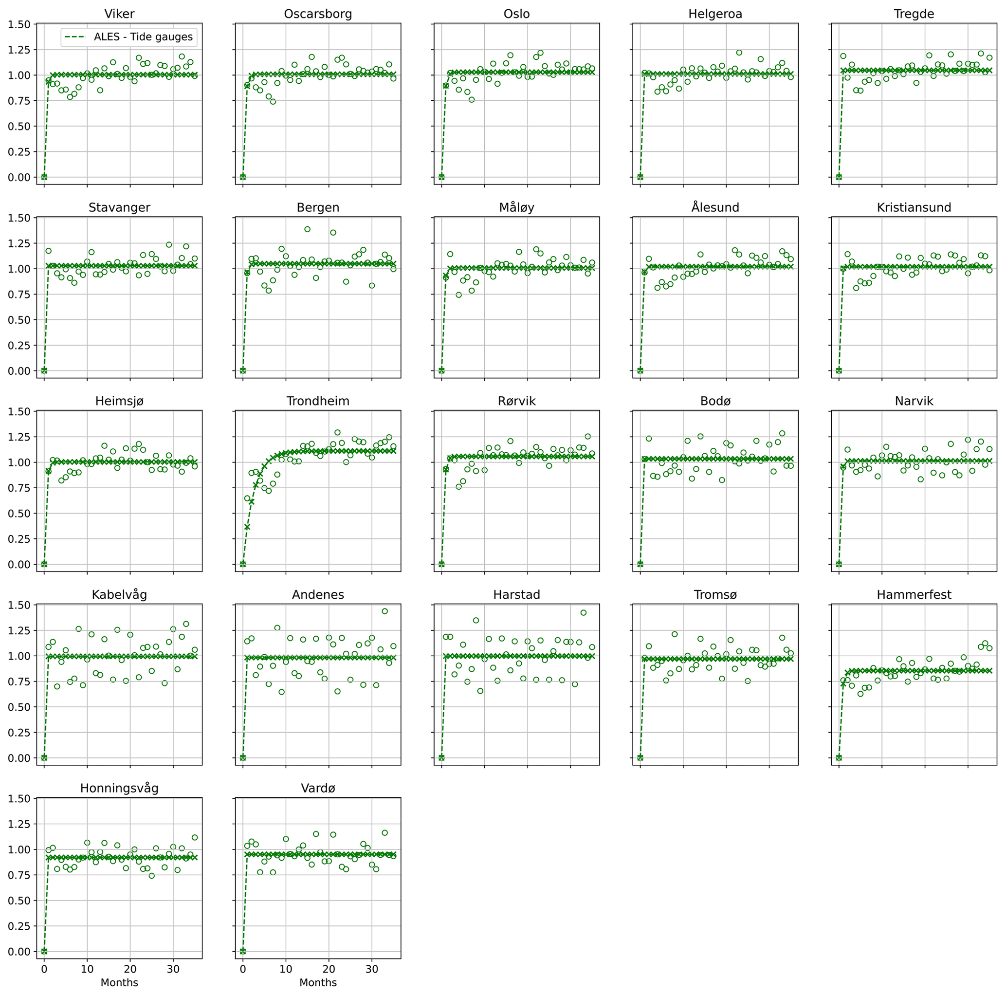
Figure A3 For each tide gauge along the Norwegian coast, semi-variogram of the difference between the detrended, deseasoned SLA estimated from the ALES-retracked satellite altimetry and from the tide gauge (empty circle) along with the corresponding fit (crosses connected by a dashed line). At each tide gauge location, we scaled each semi-variogram by the variance of the corresponding detrended and deseasoned SLA for all the plots to have the same limits on the y axis.

Appendix B

Following the same argument as in Appendix A, to estimate the uncertainty associated with the linear trends of the thermosteric, halosteric, and steric components of the sea level along the Norwegian coast (Fig. 12), we need to account for the effective degrees of freedom in the corresponding time series.

As in Appendix A, to determine the effective number of degrees of freedom, we first produce semi-variograms of the detrended and deseasoned thermosteric, halosteric, and steric components of the sea level at each hydrographic station. Then, we determine the time needed by the semi-variogram's fit to approximately reach a plateau, adopting an exponential function (see Appendix A).

The thermosteric sea level (Fig. B1) shows the strongest serial correlation. The semi-variogram of the thermosteric sea level returns lags ranging from 3 months at Indre Utsira to around 20 months at Skrova. In general, the thermosteric component of the sea level in northern Norway has fewer degrees of freedom than in the south.

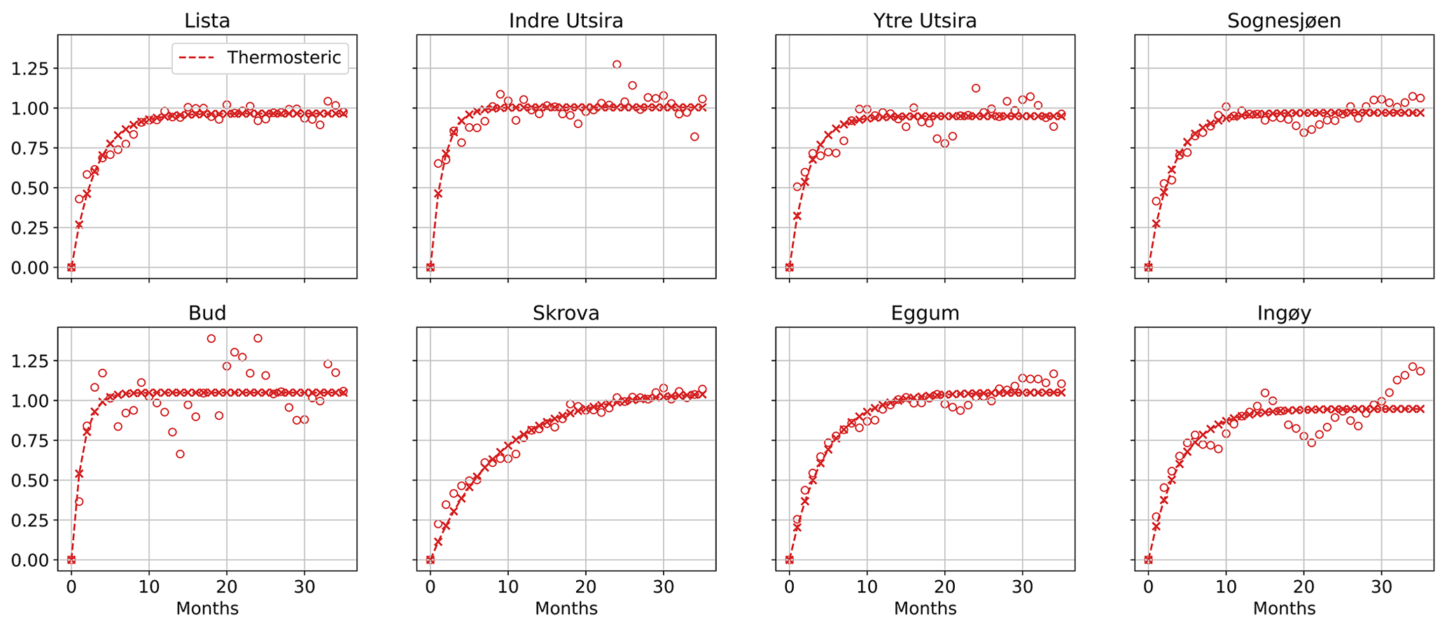
Figure B1 For each hydrographic station along the Norwegian coast, semi-variogram of the detrended and deseasoned thermosteric component of the sea-level variability (empty circles) and corresponding fit (crosses connected by a dashed line). At each hydrographic station location, we scaled each semi-variogram by the variance of the corresponding detrended and deseasoned thermosteric component of the sea level for all the plots to have the same limits on the y axis.

The halosteric (Fig. B2) and the steric (Fig. B3) components show a similar pattern, with the number of effective degrees of freedom being smaller in the north than in the south. However, both components show a weaker serial correlation when compared to the thermosteric component of the sea level. Indeed, the semi-variograms return lags between 3 and 9 months for both components of the sea level.

Similarly to Appendix A, we use Eq. (A4) to compute the 95 % confidence interval of the linear trend of the SLA and of the thermosteric, halosteric, and steric components of the sea level at each hydrographic station. With respect to Eq. (A4), though, here we only consider $N^{\ast }-\mathrm{2}$ degrees of freedom since the linear model that we use to fit the time series has only two parameters (the offset and the angular coefficient of the straight line).

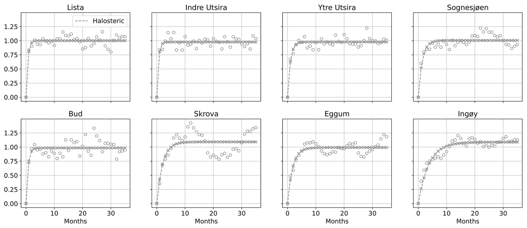
Figure B2 For each hydrographic station along the Norwegian coast, semi-variogram of the detrended and deseasoned halosteric component of the sea-level variability (empty circles) and corresponding fit (crosses connected by a dashed line). At each hydrographic station location, we scaled each semi-variogram by the variance of the corresponding detrended and deseasoned halosteric component of the sea level for all the plots to have the same limits on the y axis.

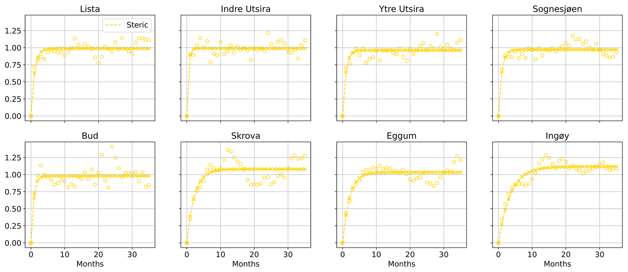
Figure B3 For each hydrographic station along the Norwegian coast, semi-variogram of the detrended and deseasoned steric component of the sea-level variability (empty circles) and corresponding fit (crosses connected by a dashed line). At each hydrographic station location, we scaled each semi-variogram by the variance of the corresponding detrended and deseasoned steric component of the sea level for all the plots to have the same limits on the y axis.

Appendix C

To compare the performance of the ALES-retracked and the conventional satellite altimetry dataset (Figs. C1, C2, C3, C4, and C5), we have downloaded the along-track L3 satellite altimetry missions provided on the Copernicus website: https://resources.marine.copernicus.eu/product-download/SEALEVEL_GLO_PHY_L3_REP_OBSERVATIONS_008_062 (last access: 2 September 2021). We should remember that the discrepancy between the two datasets might result not only from the different retrackers, but also from the different geophysical corrections applied to the data.

We select the same satellite altimetry missions that have been reprocessed with the ALES retracker, and we make sure that both satellite altimetry datasets cover the same period.

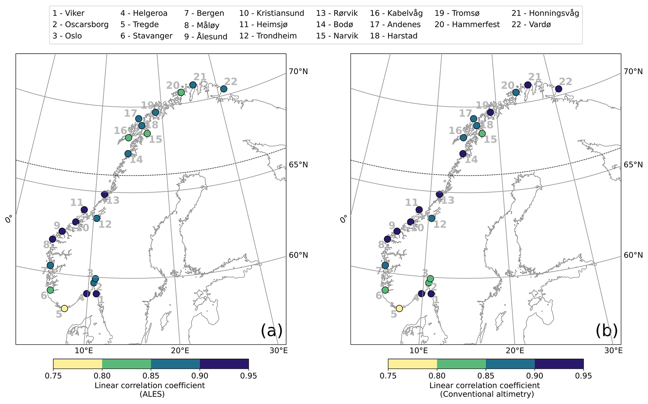
Figure C1 At each tide gauge location, linear correlation coefficient between the detrended, deseasoned monthly mean SLA estimated from the ALES-reprocessed satellite altimetry dataset and from the tide gauge (a), as well as from the conventional altimetry dataset and from the tide gauge (b). The black dashed line indicates the 66^∘ N parallel.

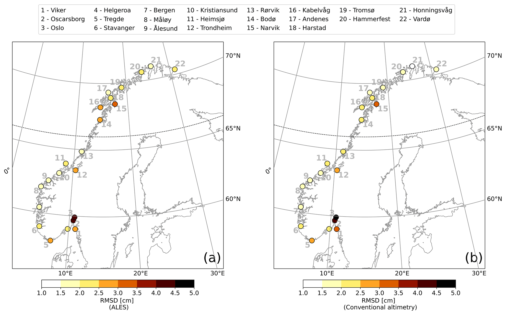
Figure C2 At each tide gauge location, RMSD of the detrended, deseasoned monthly mean SLA estimated from the ALES-reprocessed satellite altimetry dataset and from the tide gauge (a), as well as from the conventional altimetry dataset and from the tide gauge (b). The black dashed line indicates the 66^∘ N parallel.

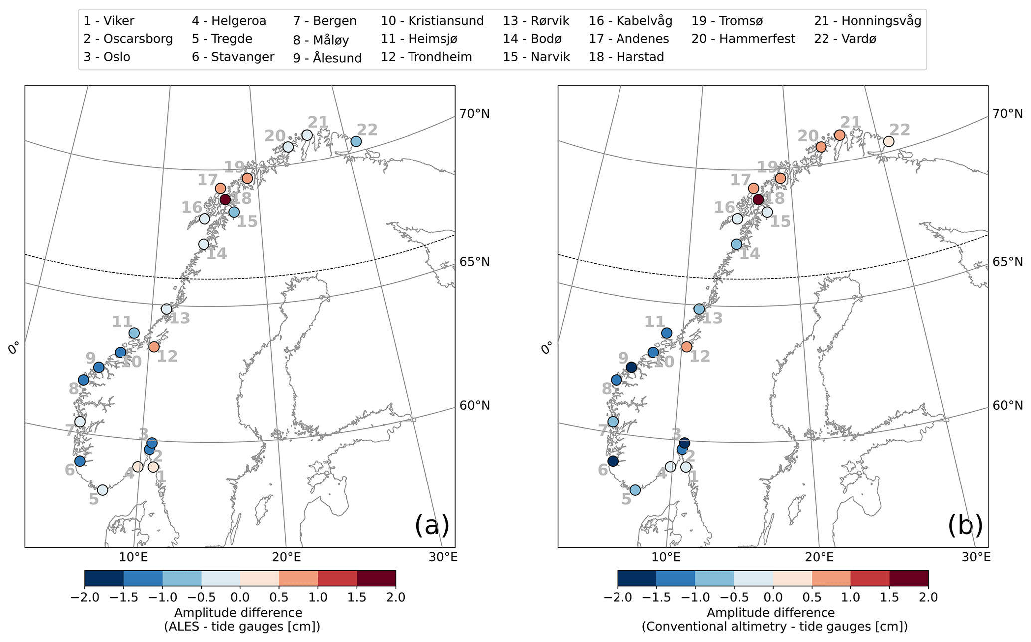
Figure C3 At each tide gauge location, difference between the amplitude of the sea-level annual cycle estimated from the ALES-reprocessed satellite altimetry dataset and from the tide gauge (a), as well as from the conventional altimetry dataset and from the tide gauge (b). The black dashed line indicates the 66^∘ N parallel.

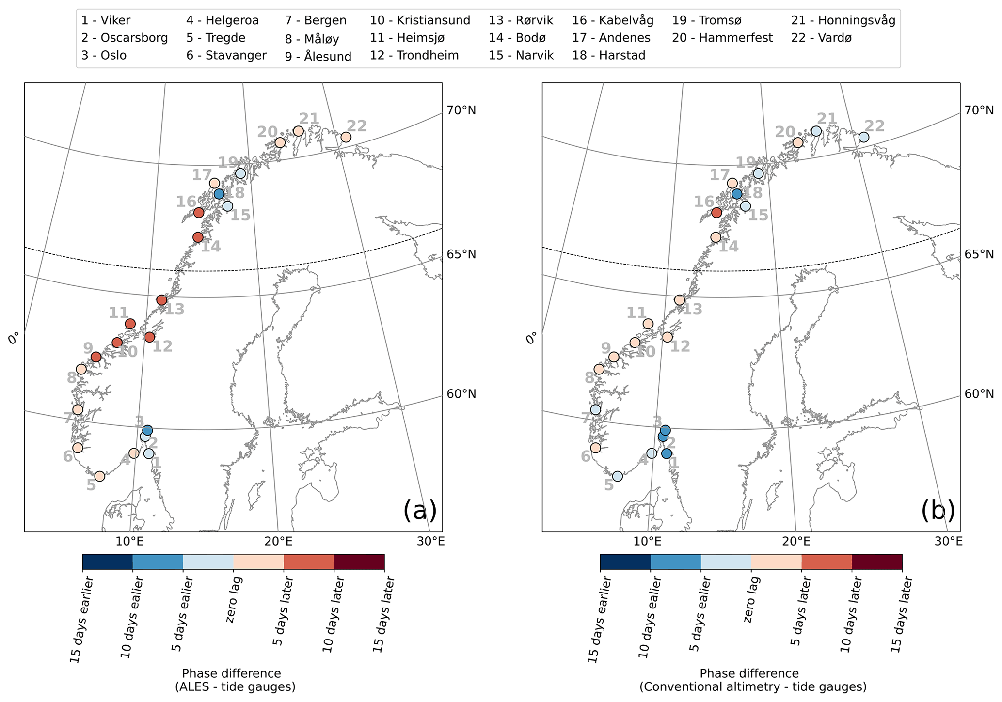
Figure C4 At each tide gauge location, difference between the phase of the sea-level annual cycle estimated from the ALES-reprocessed satellite altimetry dataset and from the tide gauge (a), as well as from the conventional altimetry dataset and from the tide gauge (b). The black dashed line indicates the 66^∘ N parallel.

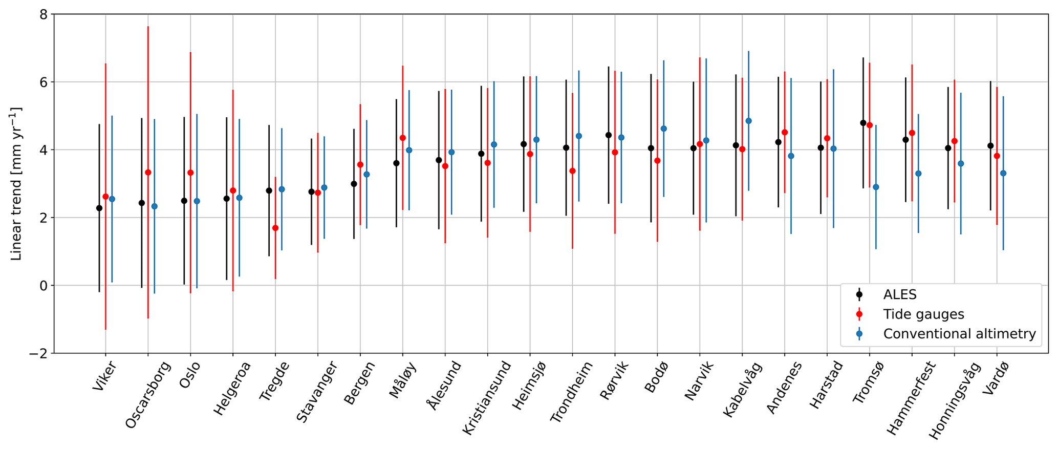
Figure C5 At each tide-gauge location, the linear trend of the SLA from the ALES-reprocessed altimetry dataset (black dots), the conventional altimetry dataset (cyan dots), and tide gauges (red dots). The error bars show the 95th confidence intervals of the sea-level trend at each tide-gauge location.