the Creative Commons Attribution 4.0 License.
the Creative Commons Attribution 4.0 License.
 | 21 Nov 2022
Ensemble quantification of short-term predictability of the ocean dynamics at a kilometric-scale resolution: a Western Mediterranean test case
Stephanie Leroux
Jean-Michel Brankart
Aurélie Albert
Laurent Brodeau
Jean-Marc Molines
Quentin Jamet
Julien Le Sommer
Thierry Penduff
Pierre Brasseur
We investigate the predictability properties of the ocean dynamics using an ensemble of short-term numerical regional ocean simulations forced by prescribed atmospheric conditions. In that purpose, we developed a kilometric-scale, regional model for the Western Mediterranean sea (MEDWEST60, at ∘ horizontal resolution). A probabilistic approach is then followed, where a stochastic parameterization of model uncertainties is introduced in this setup to initialize ensemble predictability experiments. A set of three ensemble experiments (20 members and 2 months) are performed, one with the deterministic model initiated with perturbed initial conditions and two with the stochastic model, for two different amplitudes of stochastic model perturbations. In all three experiments, the spread of the ensemble is shown to emerge from the smallest scales (kilometric scale) and progressively upscales to the largest structures. After 2 months, the ensemble variance saturates over most of the spectrum, and the small scales (<100 km) have become fully decorrelated across the ensemble members. These ensemble simulations can provide a statistical description of the dependence between initial accuracy and forecast accuracy for time lags between 1 and 20 d.
The predictability properties are assessed using a cross-validation algorithm (i.e., using alternatively each ensemble member as the reference truth and the remaining 19 members as the ensemble forecast) together with a given statistical score to characterize the initial and forecast accuracy. From the joint distribution of initial and final scores, it is then possible to quantify the probability distribution of the forecast score given the initial score or reciprocally to derive conditions on the initial accuracy to obtain a target forecast accuracy. The misfit between ensemble members is quantified in terms of overall accuracy (CRPS score), geographical position of the ocean structures (location score) and spatial spectral decorrelation of the sea surface height 2-D fields (decorrelation score). With this approach, we estimate for example that, in the region and period of interest, the initial location accuracy required (necessary condition) with a perfect model (no model uncertainty) to obtain a location accuracy of the forecast of 10 km with a 95 % confidence is about 8 km for a 1 d forecast, 4 km for a 5 d forecast and 1.5 km for a 10 d forecast, and this requirement cannot be met with a 15 d or longer forecast.
- Article
(18268 KB) - Full-text XML
- BibTeX
- EndNote


Operational services such as the Copernicus Marine Environment Monitoring Service (CMEMS) routinely provide analyses and forecasts of the state of the ocean to serve a wide range of marine scientific and operational applications. They build on state-of-the-art representations of the various dynamical components of the ocean and aim at improving the accuracy and the resolution of their products. However, with the increase in the complexity and resolution of ocean models, new questions arise regarding the predictability of the system. To what extent is it possible – and does it make sense – to forecast the very fine scales (∼ kilometric) as targeted by the future generations of these operational systems? How sensitive is such forecast to initial errors or to possible shortcomings or approximations in the model dynamics? These questions are important for operational centers because they can help to rationalize expectations for the future systems and thus help driving future developments.
Historically, the question of the predictability of dynamical systems has been addressed by considering only the irreducible sources of error, which result from intrinsic model instability combined to inevitable small initial errors. In a deterministic framework, modeling errors can indeed be excluded from the analysis because they can be reduced by additional modeling efforts, so that they do not represent a theoretical limitation on predictability. There is a long history of studies along this line, starting with Lyapunov (1992), who suggested looking for the fastest-growing unstable modes (Lyapunov vectors) and their associated e-folding timescales (Lyapunov exponents). This was extended in meteorology to describe the largest error growth over a finite time (with singular vectors, Lorenz, 1965; Lacarra and Talagrand, 1988; Diaconescu and Laprise, 2012), before it was recognized that linear instability studies were quite often not sufficient to provide a correct picture of the predictability patterns, even for quite short time lags. Nonlinear model integrations are needed to allow the fast instabilities to saturate and reveal the patterns that really matter over a given forecast time (e.g., Lorenz, 1982; Brasseur et al., 1996). For this reason, the bred vectors (Toth and Kalnay, 1993; Kalnay, 2003) have been introduced as a practical way to identify the most relevant perturbations to initialize ensemble forecasting systems. In the meantime, ensemble forecast simulations, explicitly performed with the full nonlinear model, have become the standard approach to investigate predictability (e.g., Palmer and Hagedorn, 2006; Hawkins et al., 2016). Performing an ensemble forecast amounts to propagating a probability distribution in time, which includes the possibility of a non-deterministic model. In this framework, it is thus possible to go beyond the assumption that predictability is mainly limited by unstable and chaotic behaviors and to include the possibility that intrinsic model uncertainties can be an essential limiting factor to forecast accuracy, as also recognized recently in the work of Juricke et al. (2018). In the last 2 decades, indeed, more and more studies have suggested that uncertainties are intrinsic to atmosphere and ocean models, since they cannot resolve the full diversity of processes and scales at work in the system (e.g., Palmer et al., 2005; Frederiksen et al., 2012; Brankart et al., 2015). Non-deterministic modeling frameworks have been shown to be very helpful to improve the accuracy of medium-range weather forecasts (Buizza et al., 1999; Leutbecher et al., 2017), to enhance their economical value (Palmer, 2002), to alleviate persistent biases in model simulations (Berner et al., 2012; Juricke et al., 2013; Brankart, 2013; Williams et al., 2016), and to account for some misfit between model and observations in data assimilation systems (e.g., Evensen, 1994; Sakov et al., 2012; Candille et al., 2015).
Our objective in this study is to build on a case study with a realistic high-resolution (kilometric scale) regional model, to evaluate in practice the intrinsic predictability of the ocean fine scales in this model. To do so we apply a probabilistic approach, based on ensemble simulations and on probabilistic diagnostics, from which we can assess predictability as a function of given irreducible sources of uncertainty to consider in the system.
In our approach, both the effect of initial uncertainties and model uncertainties are considered, either separately or together. We assume in both cases that they cannot be made arbitrarily small in a given operational system: initial uncertainties because observation and assimilation resources are limited and model uncertainties because model resources are limited. However, to simplify the problem, we only consider one generic type of model uncertainty that primarily affects the small scales of the system. By tuning the amplitude of the perturbations, we can simulate different levels of model accuracy and generate ensemble initial conditions with different levels of initial spread. With this assumption, we can then quantify the accuracy of the forecast that is obtained, for a given combination of initial and model uncertainties.
Reciprocally, we can expect that this set of experiments can provide insight into the maximum level of initial and model uncertainties that is required to obtain a given forecast accuracy. The objective is to help us understand the level of initial and model accuracy required to produce a useful forecast of the small scales, as targeted in the future kilometric-scale operational systems. In other words, the objective of this paper is to compute an upper bound (or more generally, necessary conditions) for the initial uncertainties, in order to obtain a targeted forecast accuracy. We do so by using different types of metrics to quantify the forecast accuracy, in order to emphasize that the definition of this metric is still a subjective choice, which depends on the goal of every particular application. The influence of one possible source of irreducible model uncertainty on this upper bound will also be illustrated. However, it is important to keep in mind that this influence will depend on the assumption made to simulate uncertainties in the system. Although generic, and designed to trigger perturbations in the small scales, they are still specific and cannot be expected to account for the full diversity of uncertainties propagating in real operational systems.
It should be emphasized that the goal of the present study remains to quantify the intrinsic predictability of the system (as defined by Lorenz, 1995) and should not be confused with that of quantifying the prediction skill of any given current operational forecasting system (e.g., Robinson et al., 2002), which would then incorporate all sources of error, such as extrinsic errors that would result from coupling with the atmosphere, sea ice, etc. However, deriving predictability as an upper bound or “necessary conditions”, as it is proposed in the present case study, can provide useful guidance for the design of the future generations of operational systems that will aim for such a kilometric resolution. As a perspective for future work, this approach could also be used in the design of a future observation network and the preparation for the assimilation of future high-resolution observations, such as wide-swath altimetry.
The paper's structure is as follows. In Sect. 2, we present the kilometric-scale regional model based on NEMO (Nucleus for European Modelling of the Ocean, Madec et al., 2002) over the Western Mediterranean sea that we set up for this study. We then introduce the parametrization for model uncertainties that is used to generate different levels of initial spread and model accuracy. In Sect. 3 we present the three ensemble experiments produced with these settings, and we assess and compare their spread growth. Predictability diagnostics are then illustrated in Sect. 4 by applying different types of metrics (probability scores, location errors, spectral analysis) to characterize the dependence of the forecast accuracy to initial and model uncertainties. We finally summarize the outcomes of this study in Sect. 5.
2.1 Model specifications and spinup
In this section, we first describe the kilometric-scale regional model of the ocean circulation based on NEMO that has been developed. It covers the Western Mediterranean sea and uses boundary conditions from a larger reference simulation (covering the entire North Atlantic) at the same resolution (eNATL60, Brodeau et al., 2020). The new regional model, MEDWEST60, covers a domain of 1200 km × 1100 km, from 35.1 to 44.4∘ N in latitude and from 5.7∘ W to 9.5∘ E in longitude (see Fig. 1). This configuration includes explicit tidal motion (tidal potential) and is forced at the western and eastern boundaries with hourly outputs from the reference simulation eNATL60 (which also includes tides). By design, all parameter choices for MEDWEST60 were made with the idea to remain as close as possible from the reference simulation eNATL60. The MEDWEST60 specifications are summarized in Table 1. We use strictly the same horizontal and vertical grids as eNATL60, meaning that there is no need for spatial interpolation of the lateral boundary conditions. Compared to the larger-domain simulation eNATL60, which was forced at the lateral boundaries by the daily GLORYS reanalysis (Lellouche et al., 2021) and an additional tidal harmonic forcing from the FES2014 dataset (Lyard et al., 2020), in MEDWEST60 we add no additional tidal forcing since it is already explicitly part of the hourly boundary forcing taken from the eNATL60 outputs. The model time step in MEDWEST60 is also increased by a factor 2 compared to eNATL60 (80 s versus 40 s, respectively).
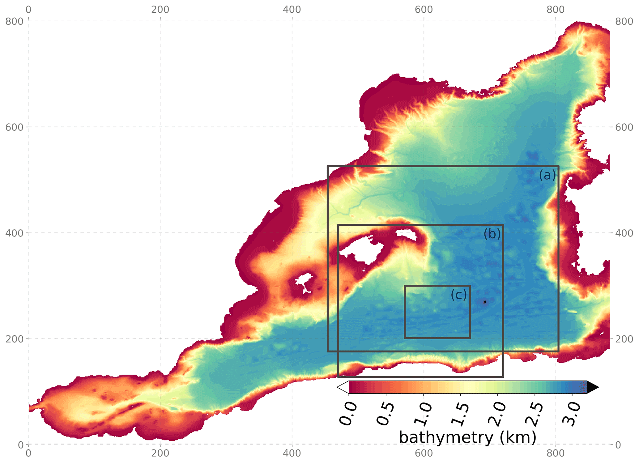
Figure 1Bathymetry (in km) of the MEDWEST60 regional domain (x and y axes are model grid points). The full domain covers 883 × 803 grid points in the horizontal, representing 1200 km × 1100 km, from 35.1 to 44.4∘ N in latitude and from 5.7∘ W to 9.5∘ E in longitude. The black squares localize three subregions which are referred to in the text and are used for various diagnostics or visualizations in the following.
Table 1Technical specifications of the MEDWEST60 model.

a The vertical levels are defined exactly as in eNATL60, but only 212 levels are actually needed to include the deepest points in the Western Mediterranean region (i.e., 3217 m at the deepest point), while 300 levels were used in eNATL60 to cover the depth range in the North Atlantic basin. The following discretization is applied to the first 20 m below the surface: 0.48, 1.56, 2.79, 4.19, 5.74, 7.45, 9.32, 11.35, 13.54, 15.89, 18.40, 21.07 m. b The flow relaxation scheme (“frs”) is used for baroclinic velocities and active tracers (simple relaxation of the model fields to externally specified values over a 12-grid-point zone next to the edge of the model domain). The “Flather” radiation scheme is used for sea surface height and barotropic velocities (a radiation condition is applied on the normal depth-mean transport across the open boundary).
By design, the MEDWEST60 model can be initialized with an instantaneous, balanced 3-D ocean state archived from the reference simulation eNATL60 on the same horizontal and vertical grids. Our spinup protocol is thus as follows: from a NEMO restart file archived from eNATL60 on a given date (here 25 January 2010), we extract the horizontal and vertical domain corresponding to MEDWEST60. A first regional simulation is then run for 5 d, started from the extracted restart file and using the same time step as eNATL60 (i.e., δt=40 s). Five more days are then run with a doubled time step of δt=80 s, and a new MEDWEST60 restart file is finally archived, to be used as the starting point on the 5 February 2010 for the following ensemble forecast experiments.
2.2 Parameterization of model uncertainties
The model presented above is a deterministic model, in the sense that the future evolution of the system is fully determined by the specification of the initial conditions, the boundary conditions and the forcing functions. This type of model – deterministic – is the archetype of the models that are currently mostly used in operational forecasting systems (though not yet at kilometric scale). In a purely deterministic approach, forecast uncertainties can only be explained by initial uncertainties, boundary uncertainties or forcing uncertainties, usually amplified by unstable model dynamics. However, as motivated in the introduction, the objective of this study is to go beyond this assumption and include the possibility of model errors impairing the predictability of the finest scales.
We thus transform the deterministic model presented above into a stochastic model, with the ambition to emulate uncertainties that primarily affect the smallest scales of the ocean flow and let them upscale to larger scales according to the model dynamics. These uncertainties are likely to depend on many possible sources, by embedding for instance misrepresentations of the unresolved scales and approximations in the model numerics but also many others. A detailed causal examination of the origin and interactions between these various possible sources of error being quite impossible to achieve, we propose to introduce here a bulk parameterization of these effects, by assuming that one of the most important dynamical consequence of these errors on the finest scales is to generate uncertainty in the location of the oceanic structures (currents, fronts, filaments …).
In fluid mechanics, there is ample literature explaining that the effect of unresolved scales in a turbulent flow can be described by uncertainties in the location of the fluid parcels (e.g., Griffa, 1996; Berloff and McWilliams, 2002; Ying et al., 2019). This general idea is applied for instance in the work of Mémin (2014) and Chapron et al. (2018), where the Navier–Stokes equations are modified by adding a random component to the Lagrangian displacement dX of the fluid parcels (as in a Brownian motion).
In the present study, location uncertainties are introduced in our ocean model according to a similar idea, but it is done differently by applying directly the random perturbations to the discrete model (rather than the mathematical equations), in the form of stochastic fluctuations in the horizontal numerical grid. In summary, the effect of the parameterization is to perturb the horizontal metrics of the model (i.e., the size of the horizontal grid cells Δx, Δy) using a multiplicative noise with specified time and space correlation structure. The stochastic perturbation is implemented using the stochastic module of NEMO (Brankart, 2013) and expresses a random second-order autoregressive process, of which we can set the amplitude (i.e., its standard deviation) and the time and space correlations. An extensive description and justification of this parameterization is developed in Appendix A.
The two main effects that this parameterization is expected to produce in the model are on the horizontal advection and on the horizontal pressure gradient. In the advection scheme, the stochastic part of the displacement dX of the fluid parcels is directly accounted for by the displacement of the grid, and in return, the transformed grid induces modifications in the advection by the resolved scales. In addition, location uncertainties also produce fluctuations in the horizontal pressure gradient (by shifting the position of the tracer fields). It is therefore expected that these stochastic fluctuations can bring a substantial limitation on the predictability of the small-scale motions. Overall, we can see indeed that non-deterministic effects are produced in several key components of the model and that all of these effects consistently derive from the sole assumption that the updated location of the fluid parcels after a model time step is not exact but approximate.
In our application, the correlation scales of the stochastic noise have been set to 1 d and 10 grid points, to be smooth enough and nonetheless produce perturbations on the small-scale side of the spectrum. The standard deviation of the noise can also be tuned, so that it is easily possible to simulate different levels of model accuracy, as required in our experiments to generate different levels of initial ensemble spread (see Sect. 3). This standard deviation must however remain small with respect to the size of the model grid cells so that the perturbations do not impair the physics of the model for the resolved scales (see Sect. 3.2). In practice, we have used values of 1 % and 5 %. Given the typical size of the model grid (1.4 km on average) and the correlation timescale of the perturbations (1 d), the typical displacement of the grid points is thus about 14 or 70 m d−1 in the two horizontal directions in the experiment with a 1 % or 5 % perturbation, respectively. The way this stochastic perturbation affects the model solution will be assessed and discussed in Sect. 3.2.
Three ensemble forecast experiments were performed with MEDWEST60, to investigate predictability as a function of both initial uncertainty and model uncertainty. In this section, we give a description of these three ensemble experiments and how they were initialized. We then assess how the spread grows with time in those ensembles, comparing the results from the stochastic model (with model uncertainty) and from the deterministic model (no model uncertainty). The predictability diagnostics will be presented in Sect. 4.
3.1 Generating the ensembles
Two experiments (ENS-1% and ENS-5%) are performed with the stochastic model (i.e., including model uncertainty) and starting from the same perfect initial conditions on the 5 February 2010. Those two ensemble experiments explore two different amplitudes of the stochastic scheme described in Sect. 2.2 and Appendix A. Experiments ENS-1% and ENS-5% are set for a stochastic perturbation of standard deviation 1 % and 5 % of the horizontal grid spacing, respectively (see illustration in Fig. 2). By design, the other parameters of the stochastic module are kept identical in all the experiments: the time correlation is set to 1 d (1080 time steps), and the Laplacian filter introducing spatial correlations is applied 10 times.
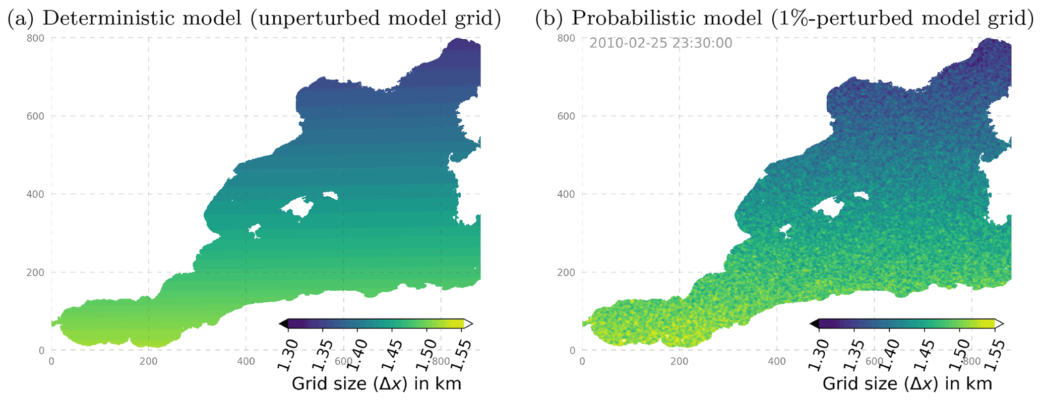
Figure 2Size of the model grid in the horizontal east–west dimension (Δx): (a) unperturbed, from the standard NEMO grid at ∘ resolution and (b) snapshot of the perturbed metric at a given date (stochastic perturbation set to a level of SD = 1 %).
The third ensemble experiment performed (ENS-CI) is the experiment with the deterministic model (i.e., no model uncertainty) to study predictability under imperfect initial conditions (ENS-IC). It is initialized from ensemble conditions taken from experiment ENS-1% after 1 d of simulation (i.e., on the 6 February 2010) when the states of the 20 members have already slightly diverged on the fine scales. Note that the choice is made to start experiment ENS-CI with small initial errors, but this experiment also virtually gives access to forecasts initialized with larger errors by considering day 1, day 2 … day 10, etc., of ENS-CI as many different start times. This approach will be applied in the predictability diagnostics proposed in the next section (Sect. 4). Following the same idea, experiments ENS-1% and ENS-5% also virtually give access to forecasts accounting both for model error and for some initial error by considering day 1, day 2, day 10, etc., of the experiments as many different virtual start times with increasing initial error.
Table 2 offers a summary of the three ensemble forecast experiments and their characteristics.
Table 2Characteristics of the three ensemble forecast experiments ENS-1%, ENS-5%, ENS-CI.
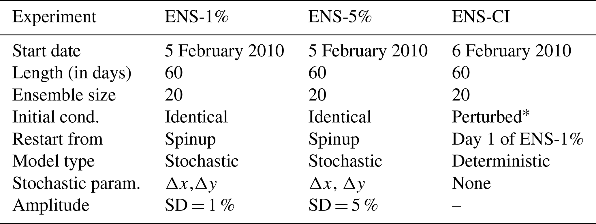
* The “perturbed” ensemble initial conditions of experiment ENS-CI are taken from the restart files of experiment ENS-1% after 1 d of simulation (see text).
3.2 Impact of the location uncertainty on the model solution
In this section, we assess how the spread grows with time in those three ensembles and how the stochastic perturbation affects the model solutions.
Note that, in our approach, the stochastic perturbation is applied on the model horizontal metrics, while the location of the grid points themselves is assumed to be the same for all members (see discussion in Appendix A). In other words, the field itself is still considered to be located on the reference grid, for instance with respect to the bathymetry and the external forcing, and the effect of the perturbation is only taken into account in the model operator (e.g., for the differential operations) and is neglected everywhere else. It implies that ensemble statistics (mean, standard deviation, covariance matrix …) can be computed as usual on the reference grid, while the perturbed metrics must be used to compute any diagnostics involving a differential operator. In the following, for instance, the perturbed metrics were used to compute relative vorticity from the velocity fields, to be consistent with the perturbed model dynamics, which is specific to each member. For that purpose, the perturbed metrics were archived with time, at the hourly frequency, in each ensemble member.
3.2.1 Wavenumber power spectrum
The stochastic scheme used in this work is designed to introduce uncertainty at the model grid scale, with a correlation length scale of 10 grid points, i.e., about 14 km. Uncertainty is thus introduced within the 10–18 km range of the Rossby radius of deformation in the region (Escudier, 2016), those scales being here resolved by ∼ 7 to 13 model grid cells. The introduced uncertainty is then expected to develop and cascade spontaneously toward larger scales through the model dynamics. The design should be such that the introduced perturbation alters the behavior of the physical quantities simulated by the model as little as possible. Figure 3 illustrates that the simulated fields in the perturbed model do indeed remain nearly unaltered and indistinguishable from the same fields in the unperturbed model. Only in the zoomed snapshot of relative vorticity (i.e., taking the Laplacian of sea surface height, thus emphasizing gradients) from the strongest perturbation experiment do some visual alterations start to appear on the smallest scales (ENS-5%, Fig. 3f). Note that this is why we did not propose any additional experiment with a stronger perturbation than 5 % in our study.
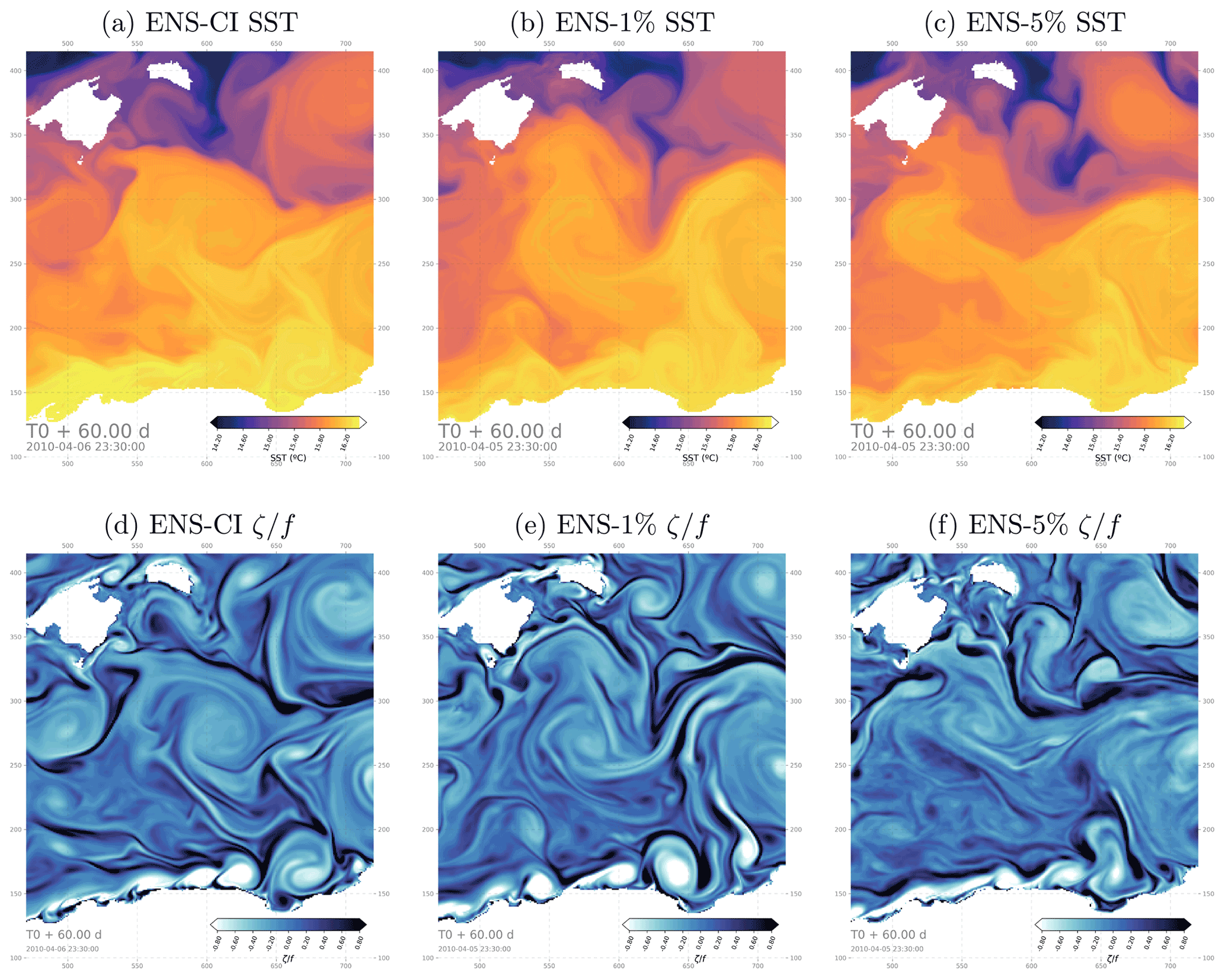
Figure 3Hourly snapshots of sea surface temperature (a–c) and relative vorticity (d–f) from one example member after 60 d in the ensemble experiments ENS-CI, ENS-1% and ENS-5% focusing on a 250×250 grid point subregion southeast of the Balearic Islands (box b in Fig. 1).
Figure 4 also confirms that the stochastic perturbation does not alter the spectral characteristics of the physical quantities in the model. It compares the wavenumber power spectrum (power spectral density, PSD) of SSH hourly snapshots from the different experiments, with or without stochastic perturbations, and also from the eNATL60 model (from which the boundary conditions were taken). On average, over the 2 months of the experiments, the figure shows very consistent SSH spectra from the perturbed and unperturbed models, giving us confidence in our designed perturbation.
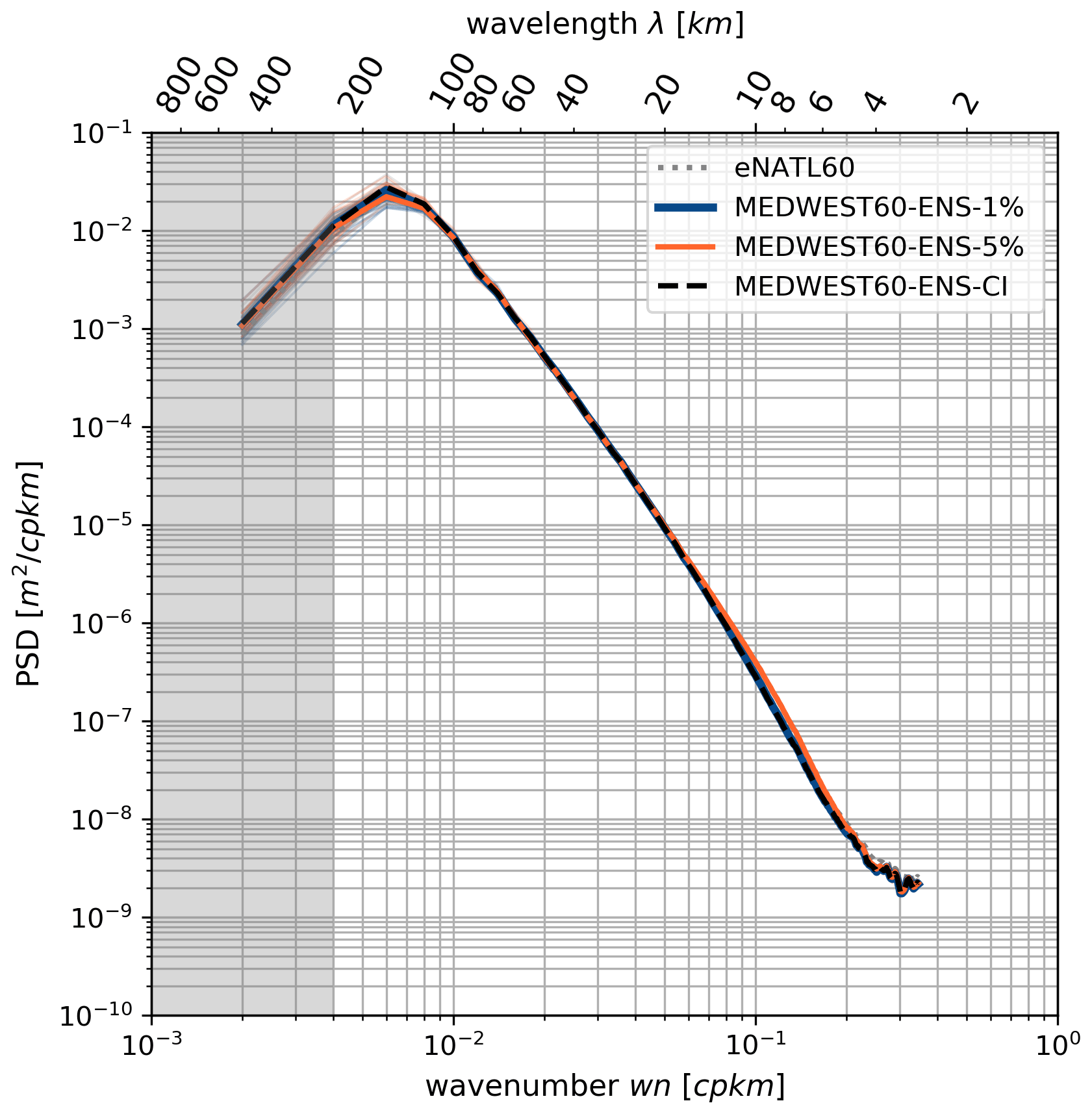
Figure 4Wavenumber spectrum (power spectral density, PSD) of hourly SSH snapshots in the MEDWEST60 ensemble experiments, in a box of 350 × 350 grid points (see box a in Fig. 1), corresponding to a size L∼490 km. Comparison is also made with the eNATL60 simulation. The PSD of SSH [m2 cpkm−1 (cpkm – cycle per kilometer)] is averaged in time over 241 hourly snapshots of SSH, 1 hourly spectrum every 6 h, over the 2 months of simulation and over all members of the given ensemble (thick lines). The PSDs of all individual members are also shown as thin lines, in the same color as their ensemble mean. The gray shading indicates where the spatial scales are not fully resolved within the considered region (scales larger than km).
Note that the spread of the PSD around the ensemble mean of each experiment is also shown by very thin lines in Fig. 4: the members all have a PSD very consistent with their ensemble mean (the spread is smaller than the thickness of the ensemble mean line) on all scales up to ∼ 150 km. For larger scales, some spread is seen between the members and it provides an idea of the sensitivity (significance) of such a spectral analysis on the last few points of the spectrum (aliasing effects). The spectra are computed here over a squared box of L∼490 km (box a in Fig. 1), and spectral scales larger than km are not well resolved (gray shading in the figure). The ensemble spread interval appearing in the figure thus provides some guidance as to how to interpret the significance of the PSD variations in this scale range and over this time period (a 2-month average here).
3.2.2 Growth of the ensemble spread
Figure 5 illustrates the evolution with time of the ensemble spread in the three ensemble experiments performed. The spread is computed here as the ensemble standard deviation of the hourly SSH, then spatially averaged over the entire MEDWEST60 domain, for each of the ensemble experiments. As expected, the ensemble spread initially grows faster in the perturbed experiment with the large model error (ENS-5%) than with the smaller model error (ENS-1%) and in the unperturbed experiment (ENS-CI). But after about 50 d of simulation, the ensemble spread of all three experiments (ENS-CI, ENS-1% and ENS-5%) has converged on a similar value. The spread is still growing at the end of the 60 d experiments, but the curves have started to flatten, suggesting that our experimental protocol was successful at initiating divergent enough ensembles on the targeted time range (2 months). The saturation of the spread was further verified by extending one of the experiments by 2 more months (not shown here). Note also that similar characteristics of the spread growth have been seen in the other surface variables (SST, SSS, relative vorticity, not shown here).
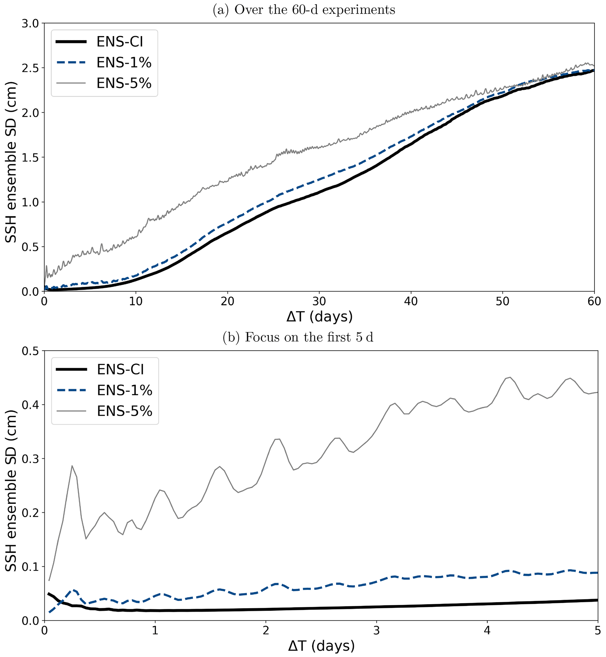
Figure 5Time evolution of the ensemble standard deviation of the hourly SSH, then spatially averaged over the entire MEDWEST60 domain for the three ensemble experiments (ENS-1%, ENS-5%, ENS-1%-S, ENS-CI): (a) over 60 d; (b) focus on the first 5 d of simulation.
After 2 months, the three experiments have reached an ensemble spread in SSH of about 2.5 cm on average over the domain, but local maxima of spread values are found around 10 cm (not shown). Further investigations discussed in the following subsection (see “Spatial decorrelation”) also confirm that the spatial decorrelation of the submeso- and mesoscale features has been reached by the end of the 2-month experiments.
After the first ∼10 d of simulation, the ensemble spread in the three ensembles evolves in a similar manner, at more or less the same rate, and almost linearly, until day 40–50, when the curves then start to flatten and converge. Only in the first few days does the presence of model uncertainty make a difference in the growth rate, ENS-5% clearly showing a faster growth than ENS-1% (the latter being slightly faster than ENS-CI in the very first few days). This result suggests that in the context of short-range forecasting (1–5 d), model uncertainties might play a role as much as uncertain initial conditions and should be taken into account in operational systems.
From Fig. 5, it appears that the presence of model uncertainty is associated with some oscillatory behavior in the ensemble spread evolution, at a period close to half a day, and with amplitude growing with the amplitude of the model error (barely visible in ENS-1% but appearing more clearly in ENS-5%). These oscillations might reflect some slight spurious numerical effects due to the horizontal grid distortions imposed in these experiments with the parametrization. The period close to tidal or inertial period might suggest some effect related to partial wave reflection in the buffer zone at the lateral boundaries of the domain, but further investigation would be needed to be able to draw any conclusions.
Note also that these experiments are initiated in the winter time (February) when mesoscale activity is expected to be the largest in the region. We have also performed an additional test experiment (not shown), identical to ENS-1% except for the start date, taken in August, when mesoscale activity is expected to be low. We found that the growth of the ensemble spread in this case is significantly slower than with winter initial conditions. It is consistent with the idea that the seasonal level of mesoscale turbulence plays a significant role in the ensemble spread of the forecast and thus in the quantification of predictability. In this paper we do not investigate the dependence on seasonality, as our main objective is to propose a methodology to quantify predictability as a function of both initial uncertainty and model uncertainty. We thus choose to focus on the winter season where the dynamics of the system are expected to maximize the growth of the ensemble spread for a given initial uncertainty.
3.2.3 Spatial decorrelation
Figure 6 illustrates how the relative vorticity fields diverge with time in hourly snapshots from two different members of experiment ENS-CI. The focus here is on a 250×250 grid point subregion in order to better emphasize the smallest simulated ocean features. At a short time lag (+1 d), the ocean states in the two example members are barely distinguishable from each other. With a +20 d time lag, differences start to appear in the exact location of the small features and their shape. After 60 d, the differences have become more obvious even on larger features and eddies, and many features do not even have a corresponding feature in the other member. At the end of the experiment, the ocean state of the two members appears clearly distinct from each other.
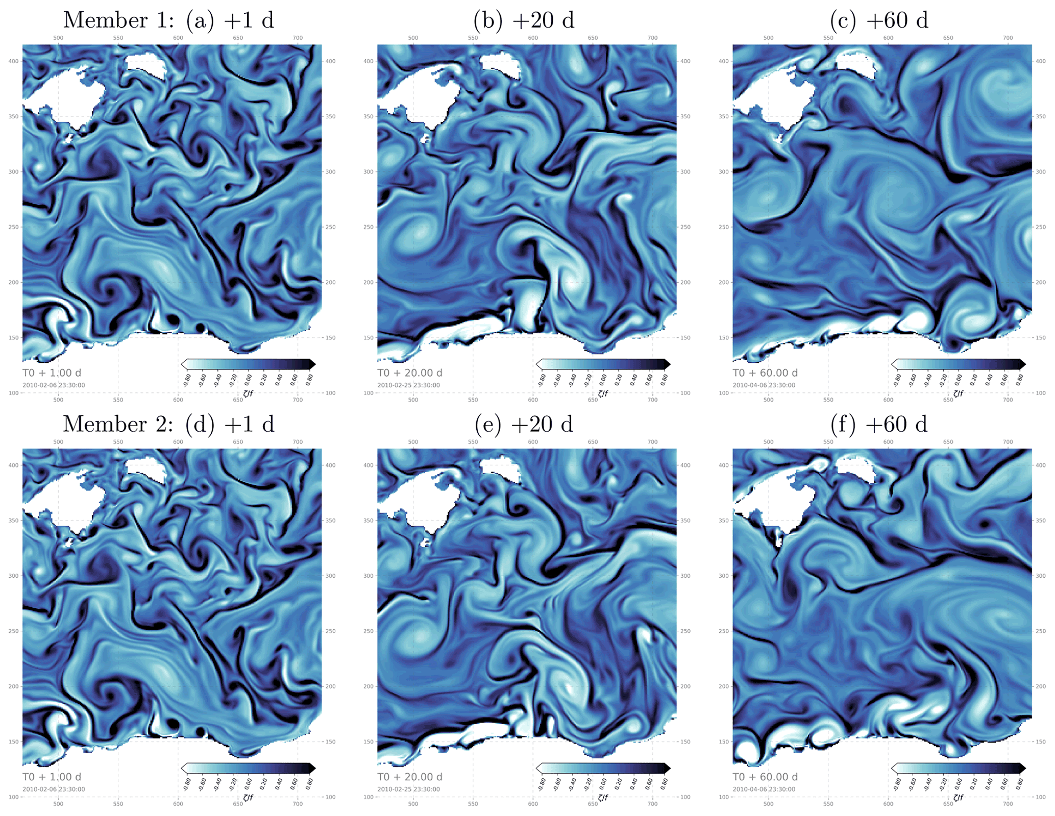
Figure 6Hourly snapshots of relative vorticity from two example members (top and bottom, respectively) after 1, 20 and 60 d (from left to right, respectively) in the ensemble experiment ENS-CI, focusing on a 250 × 250 grid point subregion southeast of the Balearic Islands (box b in Fig. 1).
In order to investigate more systematically the evolution with time of the spread between the members of an ensemble and its wavenumber spectral characteristics, we now consider the forecast “error”, which we assess here as the difference in SSH hourly snapshots taken between all pairs of members in the ensemble and at each time lag. In other words, each member is alternatively taken as the truth and compared to the 19 remaining members, taken as the ensemble forecast for that given truth. We then compute the power spectral density (PSD) of each pair difference at each time lag and then average over the 20×19 permuted pairs to obtain the systematic error. Figure 7 presents this mean PSD, characterizing the systematic forecast error, as a function of forecast time lag, in all three ensemble experiments. For reference, the ensemble-mean PSD of the full-field SSH at time lag +60 d is also plotted in the same figure.
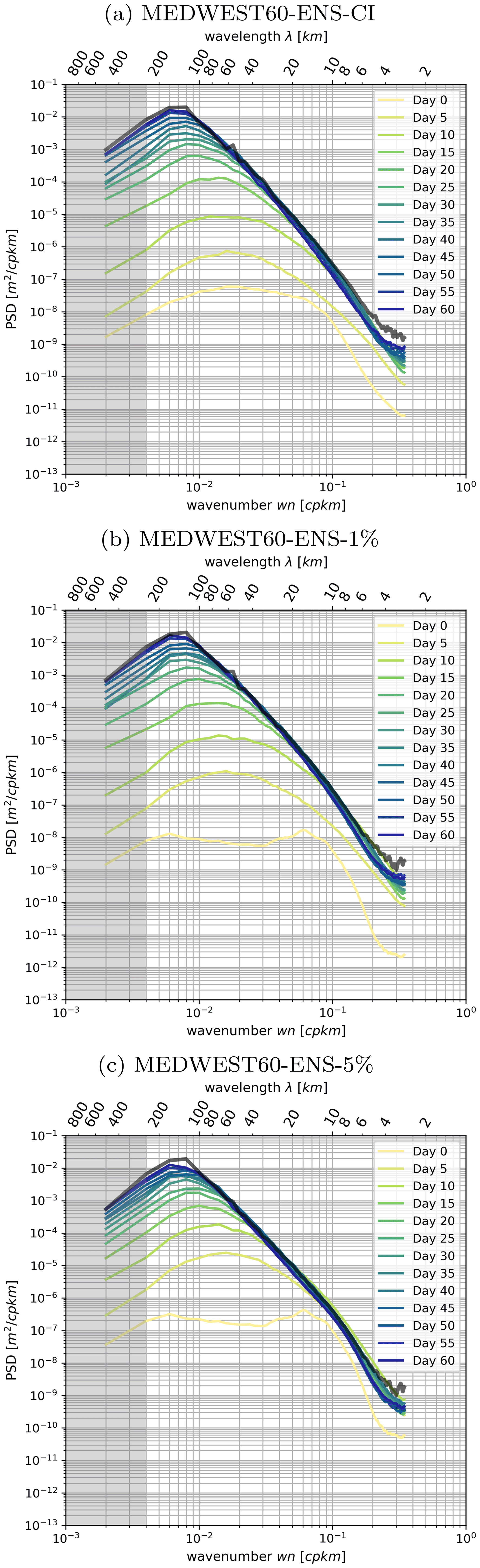
Figure 7Ensemble-mean wavenumber power spectrum density (PSD) of the hourly SSH at day 60 (black thick line) compared to the mean PSD of the forecast error in experiments (a) ENS-CI, (b) ENS-1% and (c) ENS-5%. The forecast error is assessed as the difference in the hourly SSH fields between all pairs of members in the given ensemble, and the mean is taken of the PSDs of all the 20×19 permuted pairs at each time (time increasing from yellow to blue colors); see text in Sect. 4.3 for more details. The time lag labeled “Day 0” is taken after 1 h of the experiment. The gray shading indicates where the spatial scales are not fully resolved within the considered region (scales larger than km).
After just 1 h of simulation starting from perfect initial conditions with the stochastic model in ENS-1% (yellow curve in Fig. 7b), the wavenumber spectrum of the forecast error peaks in the small scales around λ=15 km and is still 2 orders of magnitude smaller than the level of spectral power in the full-field SSH (shown as reference as a thick black line in the figure). The same behavior is observed for ENS-5% (Fig. 7c), except that the level of spectral power is 1 order of magnitude larger than in ENS-1% (since the spread grows faster in ENS-5% than in ENS-1%). With increasing time lag, the shape of the PSD becomes more “red”, with more spectral power cascading to the larger scales. By the end of all three experiments (+60 d time lag), the PSD of the forecast error has almost converged on the reference full-field SSH PSD, suggesting that the members of each ensemble have become decorrelated on the spatial scale range considered here, i.e., 10–200 km. Note that we do not necessarily expect a full spatial decorrelation between the members in this type of experiment since all members see the same surface forcing and lateral boundary conditions. From Fig. 7 it is also noteworthy that the evolution in time of the forecast-error spectrum in ENS-CI (Fig. 7a) and ENS-1% (Fig. 7b) is very similar in amplitude and shape, except for the first time lag (+1 h), where the curve in ENS-CI is already smoother than in ENS-1% and does not show the λ=15 km peak as in the latter. This is because ENS-CI is by design started from initial conditions from day +1 of ENS-1% (see Sect. 3). In any case, by a time lag of 5 d, both ENS-CI and ENS-1% have converged into a very similar forecast-error spectrum and evolve in the same manner.
Overall, we thus find that after 2 months, the ensemble variance saturates over most of the spectrum, and the small scales (<100 km) have become fully decorrelated between the ensemble members. This set of ensemble simulations is thus confirmed to be appropriate to provide a statistical description of the dependence between initial accuracy and forecast accuracy for time lags between 1 and 20 d, consistently with the diagnostics proposed in the following.
In this section, we present predictability diagnostics where we quantify predictability, based on a given forecast score measuring both the initial and forecast accuracy. Although any specific score of practical significance could have been used, we focus here on a few simple and generic scores characterizing the misfit between ensemble members, in terms of (1) overall accuracy (Sect. 4.1: Probabilistic score), in terms of (2) geographical position of the ocean structures (Sect. 4.2: Location score) and in terms of (3) spatial decorrelation of the small-scale structures (Sect. 4.3: Decorrelation score).
4.1 Probabilistic score
A standard approach to evaluate the accuracy of an ensemble forecast using reference data (Candille and Talagrand, 2005; Candille et al., 2007) is to compute probabilistic scores characterizing the statistical consistency with the reference (reliability of the ensemble) and the amount of reliable information it provides (resolution of the ensemble). For instance, in meteorology, ensemble forecasts can be evaluated a posteriori using the analysis as a reference. In the framework proposed in this study, a consistent approach to assess predictability is thus to compute the probabilistic scores that can be expected for given initial and model uncertainty. In this case, we can use one of the ensemble members as a reference, by assuming that it corresponds to the true evolution of the system, and then compute the score using the remaining ensemble members as the ensemble forecast to be tested. Furthermore, by repeating the same computation with each ensemble member as a reference, as in a cross-validation algorithm, we can obtain a sample of the probability distribution for the score. All members of the ensemble are thus used successively as a possible truth, for which the other members provide an ensemble forecast. This procedure is very similar to the ensemble approach introduced in Germineaud et al. (2019) to evaluate the relative benefit of observation scenarios in a biogeochemical analysis system. In this framework, the probabilistic score can be viewed as a measure of the resulting skill of a given observation scenario.
4.1.1 CRPS score
A common measure of the misfit between two probability distributions of a one-dimensional random variable x is the area between their respective cumulative distribution functions (CDFs) F(x) and Fref(x):
In our application, the reference CDF Fref(x) is a Heaviside function increasing by 1 at the true value of the variable, and the ensemble CDF F(x) is a stepwise function increasing by at each of the ensemble values (where m is the size of the ensemble). Thus the further the ensemble values from the reference, the larger Δ, and the unit of Δ is the same as the unit of x.
The continuous rank probability score (CRPS) is then defined (Hersbach, 2000; Candille et al., 2015) as the expected value of Δ over a set of possibilities. In practical applications, the expected value is usually replaced by an average of Δ in space and time. In our application, the cross-validation algorithm would give the opportunity to make an ensemble average and thus be closer to the theoretical definition of CRPS. However, the ensemble size is too small here to provide an accurate local value of CRPS, so that we prefer computing a spatial average as would be done in a real system and compute an ensemble of spatially averaged CRPS scores. In the following, CRPS scores will be computed by averaging over a subregion of the domain basin southeast of the Balearic Islands (100×100 grid point region labeled as box c in Fig. 1).
4.1.2 Evolution in time
We first investigate the ensemble experiment performed with the deterministic model and uncertain (i.e., perturbed) initial conditions (ENS-CI). The additional effect of model uncertainties will be diagnosed in a second step.
Figure 8 shows the time evolution of the CRPS score for SSH, SST and SSS as obtained in experiment ENS-CI. It is computed for each of the 20 permuted cases taking an ensemble member as the reference truth and the rest of the members as the ensemble forecast. The CRPS score starts from 0 and the initial increase is about exponential, with a doubling time of about 4 d. After typically 20 d, the evolution of the score becomes more irregular, globally increasing but also sometimes decreasing in time, depending on the particular situation of the system. During the initial exponential increase, the diversity of possible evolutions of the score remains moderate: the score only increases a bit faster or a bit slower according to the member that is used as a reference. In the second period, however, the evolution becomes very diverse, with the score sometimes increasing with time for a given reference member and decreasing for another reference member. This shows the importance of accounting for the diversity of possible situations in the description of predictability. With time, anomalous situations can emerge, which can produce different predictability patterns. Predictability thus needs to be described as a probability distribution of the score for given conditions of initial uncertainty (and/or of model uncertainty).
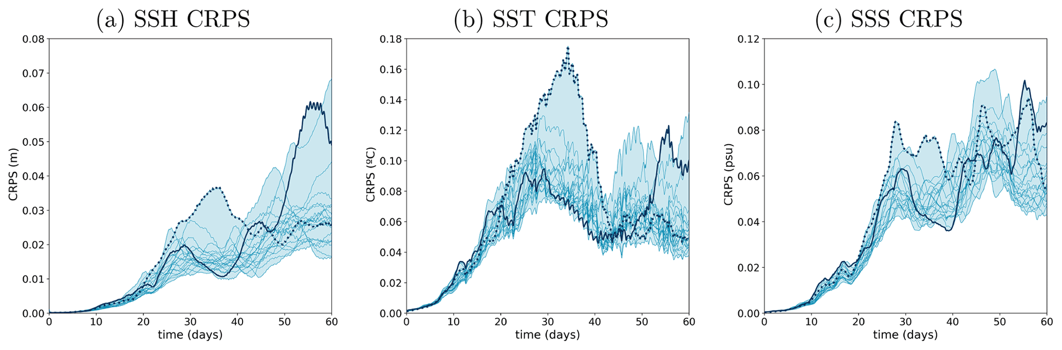
Figure 8Time evolution of the CRPS score (y axis) for SSH (meters), SST (degree Celsius) and SSS (psu) from experiment ENS-CI. The score is computed for each of the 20 permuted cases (thin lines) taking an ensemble member as the reference truth and the rest of the members as the ensemble forecast. The blue shading represents the minimum-to-maximum envelop of the 20 scores computed for the experiments. Two example lines are plotted thicker (solid and dotted lines) in each panel to illustrate how individual scores can evolve with time.
4.1.3 Predictability diagrams
Using the time evolution of the ensemble CRPS score obtained in the previous section, it is then possible to describe predictability for a given time lag Δt by the joint distribution of the initial and final score CRPS(t) and CRPS(t+Δt), respectively. From this distribution, we can indeed obtain the conditional distribution of the final score given the initial score and reciprocally the conditional distribution of the initial score required to obtain a given final score.
Figure 9 describes predictability for three time lags Δt=2, 5 and 10 d, for SSH, SST and SSS, by plotting the forecast CRPS score (y axis) conditioned on the initial CRPS score (x axis) of the same variable. The figure is plotted for experiment ENS-CI, i.e., without model uncertainty. It is in fact just a reshuffling of the data from Fig. 8, gathering all couples of scores with time lag Δt. It must be kept in mind that the figure mixes forecasts starting at a different initial time (in the range of the 2-month experiment), which can correspond to various situations of the system, in particular to different atmospheric forcings. The resulting probability distribution thus encompasses this set of possibilities, the only conditions being on the time lag Δt and the initial CRPS score. To put a condition on the initial time would have required performing a large number of ensemble forecasts from that initial time with various levels of initial error and would have been far too expensive.
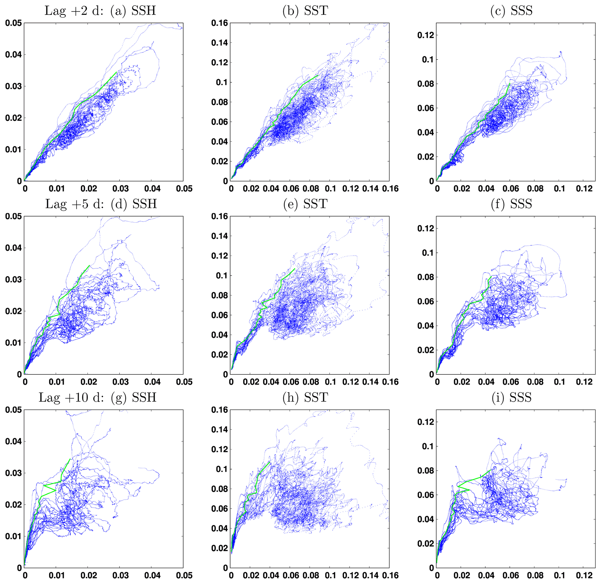
Figure 9Final CRPS score (y axis) as a function of the initial CRPS score (x axis), for three time lags Δt=2, 5, and 10 d (from top to bottom) for SSH (meters), SST (degree Celsius) and SSS (psu). The green line corresponds to the initial score required to have a 95 % probability that the final score is below a given value.
The first thing to note from Fig. 9 is that for a given initial score, there can be a large variety of final scores after a Δt forecast, which again shows the importance of a probabilistic approach. What we obtain is a description of the probability distribution of the final score given the initial score or, reciprocally, the probability distribution of the initial score to obtain a required final accuracy. These are just two different cuts (along the y axis or along the x axis) in the two-dimensional probability distribution displayed in the figure. From this probability distribution, it is then possible to compute the initial score required to have a 95 % probability that the final score is below a given value (with imperfect accuracy where the spread is large, as a result of the limited size of the ensemble). This result, corresponding to the green curve in the figure, can be viewed as one possible answer to the question raised in the introduction about the initial accuracy required to obtain a given forecast accuracy.
4.1.4 Effect of model uncertainties
To explore the potential additional effect of model uncertainties (as represented by the stochastic scheme described in Sect. 2.2) on predictability, we can compare the CRPS diagnostics described above for the three ensemble experiments performed: ENS-CI (no model uncertainty), ENS-1% (moderate model uncertainty) and ENS-5% (larger model uncertainty). To that end, Fig. 10 shows the time evolution of the CRPS score for these three experiments. We observe that forecast uncertainty increases faster with model uncertainty included in the system (especially in ENS-5%), although the asymptotic behavior of the score is very similar in all three simulations. Model uncertainty mainly matters for a short-range forecast (less than ∼15 d) when the initial condition is very accurate. Of course, this conclusion only holds for the kind of location uncertainty that we have introduced in NEMO here, with short-range time and space correlation. A long-standing effect of model uncertainty on predictability would be expected for large-scale perturbations, as in the atmospheric forcing, for example (in this study though, we do not consider atmospheric forcing uncertainty, as the ocean model is forced by a prescribed and presumably “true” atmosphere).
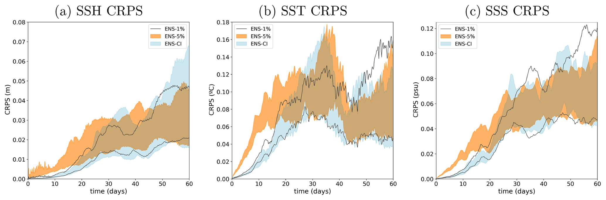
Figure 10CRPS score as a function of time for (a) SSH (meters), (b) SST (degree Celsius) and (c) SSS (psu), compared for the three simulations: ENS-CI (no model uncertainty, blue shading), ENS-5% (larger model uncertainty, orange shading) and ENS-1% (small model uncertainty, gray lines). Only the minimum-to-maximum envelop of all the 20 individual CRPS scores is represented for each experiment (the 20 individual scores are omitted).
The consequence of this specific impact of model uncertainty is that the predictability diagrams displayed in Fig. 9 remain very similar for all three experiments, only becoming a bit more fuzzy when model uncertainty is included. To see the difference, we need to focus on the short time lag (Δt=2 d) and on the small initial and final scores (which correspond to the beginning of the experiments). Figure 11 compares the results obtained for SSH in ENS-CI, ENS-1% and ENS-5%, and we can observe that with larger model uncertainty, a smaller initial score (i.e., a more accurate initialization from observations) is generally needed to obtain a given final score (i.e., a given target of the forecasting system). If this model uncertainty is irreducible (as argued in Sect. 2.2 if it represents the effect of unresolved scales), it can thus represent an intrinsic limitation on predictability (at that resolution), at least in the specific case of a short time lag and a small initial error.
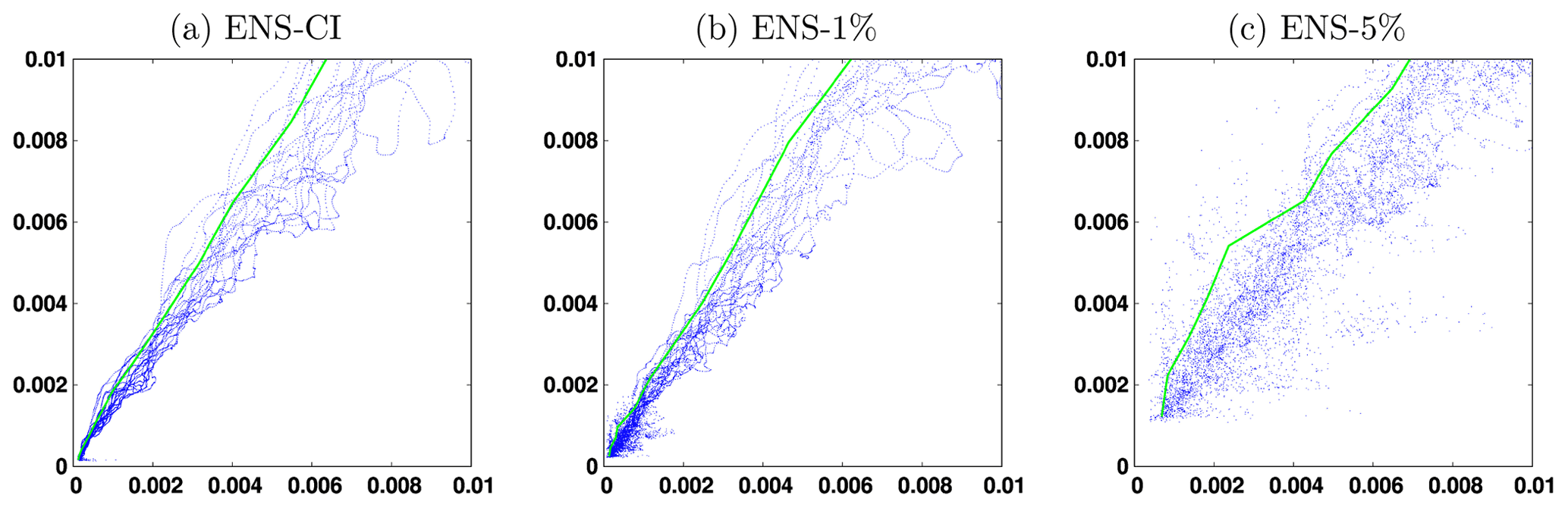
Figure 11Forecast CRPS score (y axis) as a function of the initial CRPS score (x axis) for SSH (meters) at time lag Δt=2 d. The green line corresponds to the initial score required to have a 95 % probability that the final score is below a given value. The figure compares the three simulations (a) ENS-CI (no model uncertainty), (b) ENS-1% (small model uncertainty) and (c) ENS-5% (larger model uncertainty) for the small CRPS scores (smaller than 0.01 m).
4.2 Location score
In the previous section, a probabilistic score has been used to describe the accuracy of the initial condition that can be associated with any given observation or assimilation system. However, in many applications, what matters is not so much the accuracy of the value of the ocean variables, but the location of the ocean structures (fronts, eddies, filaments …). Moreover, the acuteness of the positioning of ocean structures that can be obtained in the initial condition of the forecast can be thought to be rather directly related to the resolution of the observation system that is available for the operational forecast (in situ network or satellite imagery).
For these reasons, in this section, we will introduce a simple measure of location uncertainties in an ensemble forecast, which will be used in the same way as the CRPS score in the previous section. The same type of diagnostics will be computed to provide a similar description of predictability but from a different perspective.
4.2.1 Misfit in field locations
To obtain a simple quantification of the position misfit between two ocean fields (one ensemble member and a reference truth), we are looking for an algorithm to compute at what distance the true value of the field can be found. Ideally, what we would like is to find the minimum displacement that would be needed to transform a given ensemble member into the reference truth. However, it is important to remark that this does not amount to computing the distance between corresponding structures in the two fields. This would indeed require an automatic tool to identify coherent structures in the two fields and would be much more difficult to achieve in practice. In general, if the two fields are not close enough to each other, such an identification would even be impossible, since ocean structures can merge, appear, disappear or be transformed to such extent that no one-to-one correspondence can be found.
In addition, to further simplify the problem, we do not consider the original continuous fields but modified fields that have been quantized on a finite set of values. Figure 12, for instance, shows the salinity field from two example members of the ENS-CI simulation (after 15 d), together with their quantized version. The quantized version is obtained by computing the quantiles of the reference truth, for instance 19 quantiles here (from the distribution of all values in the map), and then by replacing the value of the continuous field by the index of the quantile interval to which it belongs (between 1 and 20). In this case, a value of 1 means that the field is below the 5 % quantile and a value of 20 means that the field is above the 95 % quantile. From these quantized fields, it is then easy to find the closest point where the index is equal to that of the reference truth and thus where the field itself is close to the truth (to a degree that can be tuned by changing the number of quantiles).
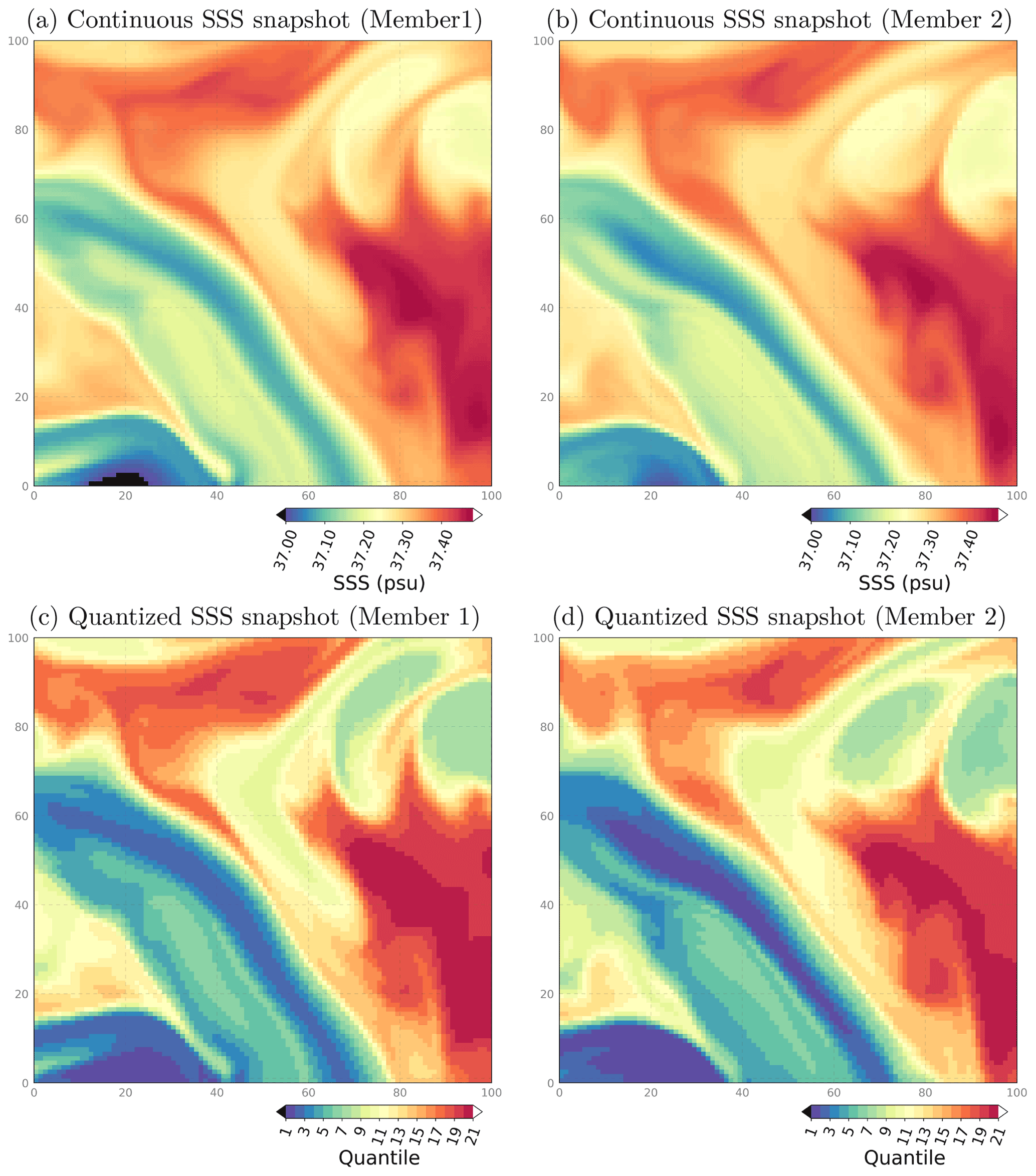
Figure 12Surface sea salinity (SSS) hourly snapshots from two example members of experiment ENS-CI after 15 d, focusing on a 100 × 100 subregion southeast of the Balearic Islands: box (c) in Fig. 1. The original continuous fields are shown in the top row (a, b) and their quantized version (c, d) in the bottom row.
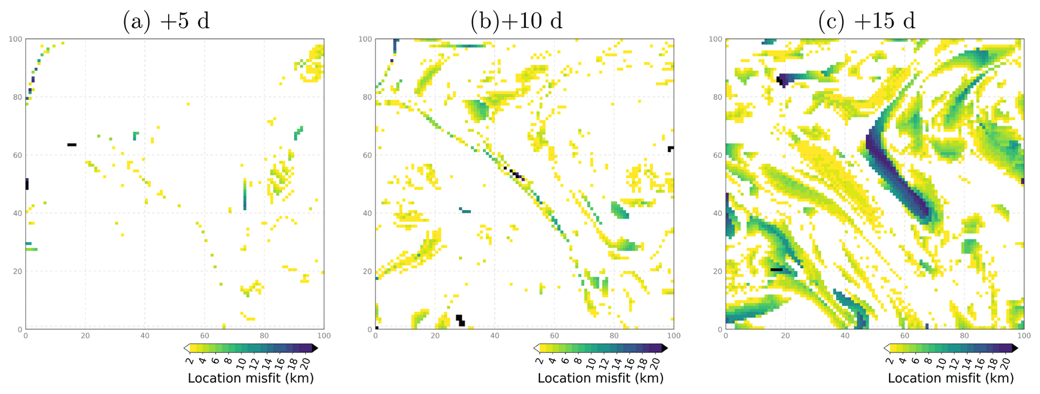
Figure 13Location misfit (in km) between the surface salinity fields of two example members in the ensemble experiment ENS-CI after 5, 10 and 15 d (from left to right), focusing on a subregion southeast of the Balearic Islands: box (c) in Fig. 1.
Figure 13 shows the resulting maps of location misfit, in kilometers, for salinity in ENS-CI after 5, 10 and 15 d. We see that the location misfit increases with time as the two ensemble members diverge from each other. At +10 d, misfit values of 5–10 km are sparsely seen in the SSS field, featuring a thin elongated pattern that likely illustrates the arising misfit in the location of a NW–SE front (sharp gradient in the SSS field, as seen in Fig. 12c–d). At +15 d, the location misfit has increased in amplitude and now covers most of the subregion, with maximum values of 15–20 km. From such maps, it is then possible to define a single score from the distribution of distances. For the purpose of this study, we simply define our location score as the 95 % quantile of this distribution, which means that location error has a 95 % probability of being below the distance given by the score.
4.2.2 Evolution in time
We start by analyzing the time evolution of the location score in ensemble experiment ENS-CI, where the only source of uncertainty comes from the initial conditions (no model uncertainty; the model is deterministic). Figure 14 shows the evolution in time of the location score for SST and SSS, considering each pair of members in the ensemble, which amounts to a total of curves displayed in the figure. The two panels, for (a) SST and (b) SSS, both show a similar distribution of the time evolutions, confirming that our quantification of location uncertainty is consistent for these two tracers. Figure 14 also shows that during about the first half of the experiment (the first 30 d), the location score increases towards saturation, with a spread that also increases with time, whereas in the second half of the experiment, the score has reached the asymptotic distribution, which is characterized by a large location uncertainty and a large spread of the score. It means that there is no more information about the location of the ocean structures in the forecast and that the score can be either moderate (down to 20 km) or very large (up to 80 km and more) depending on chance. In the following, we thus mostly focus on the range of scores, between 0 and 20 km, where a valuable forecast accuracy can be expected (for the small-scale tracer structures that are resolved by the model).
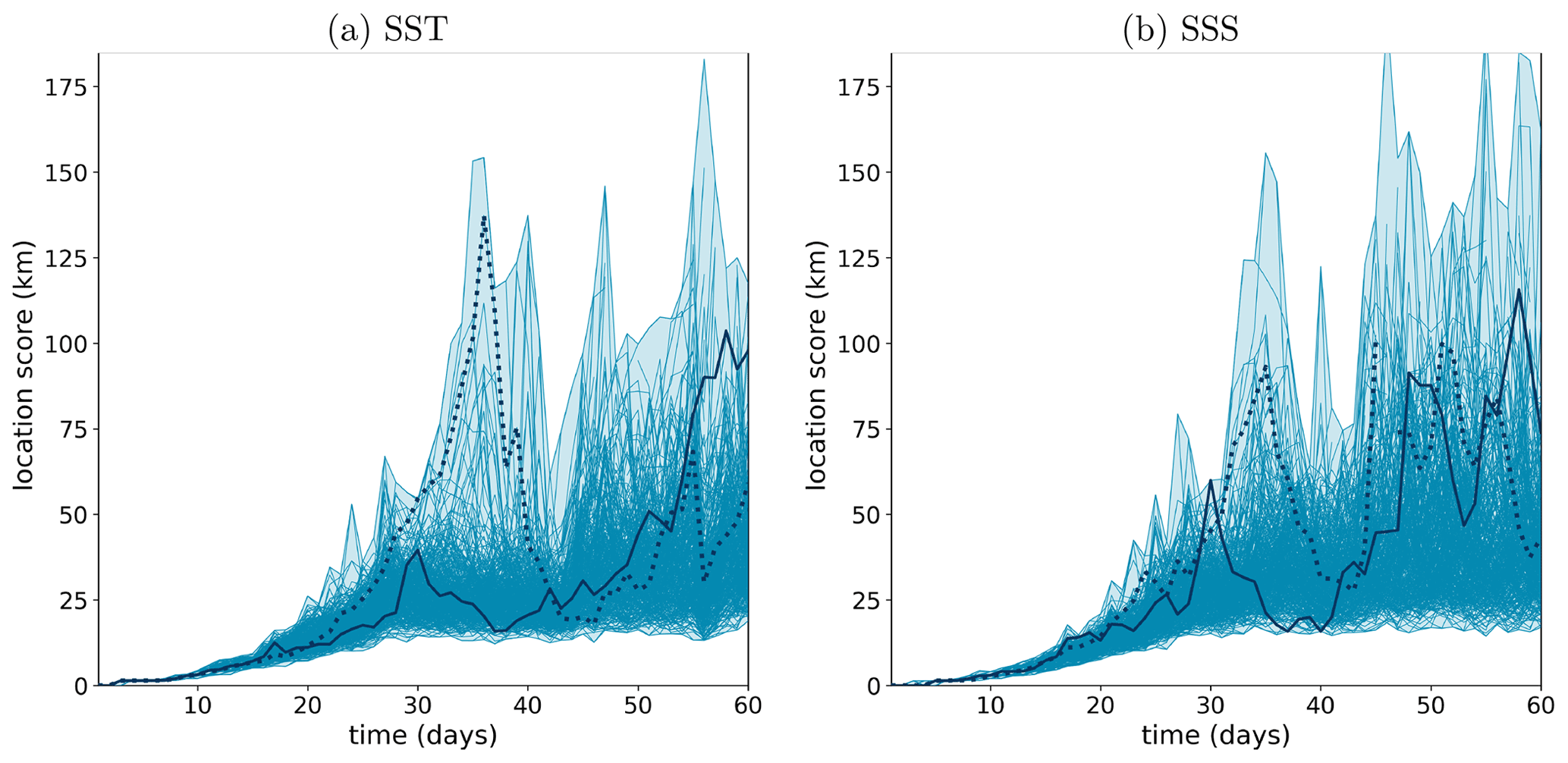
Figure 14Time evolution of the location score (y axis, in km) for (a) SST and (b) SSS in experiment ENS-CI. The score is computed for each of the 20×19 permutated pairs (blue lines) considering one ensemble member as the reference truth and each of the 19 remaining ensemble members as a forecast. The blue shading represents the minimum-to-maximum envelop of all the 20×19 scores computed for the experiment. Two example lines are plotted thicker (solid and dotted lines) in each panel to illustrate how individual scores can evolve with time.
4.2.3 Predictability diagrams
From the time evolution of the score described in the previous section, we can then deduce predictability diagrams, following exactly the same approach as for CRPS in Sect. 4.1.3. Figure 15 describes predictability (computed from SST fields) for six time lags (Δt=1, 2, 5, 10, 15 and 20 d), by showing the final location score (y axis) as a function of the initial location score (x axis). Again, this figure is just a reshuffling of the data from Fig. 14, gathering all couples of scores with time lag Δt, using the same assumption already discussed in Sect. 4.1.3. Note that the longest time lags considered here (>10 d) are relevant only in the present context of forced ocean experiments (as a forecasted atmosphere would also become a major source of uncertainty for ocean predictability in a real operational forecast context at those time lags).

Figure 15Final SST location score (y axis, in km) as a function of the initial SST location score (x axis, in km) for experiment ENS-CI for six time lags Δt=1, 2, 5, 10, 15 and 20 d (from a–f). The green line corresponds to the initial score required to have a 95 % probability that the final score is below a given value.
The interpretation of Fig. 15 follows the same logic as the previously discussed predictability diagrams for CRPS. But the structure of the diagrams is even more directly understandable here, and the loss of predictability with time appears more clearly. For instance, if one seeks a forecast accuracy of 10 km with a 95 % confidence (i.e., a y value of the green curve equal to 10 km), then Figure 15 shows that the initial location accuracy required (necessary condition but not sufficient; see the “Summary and conclusion” section) is about 8 km for a 1 d forecast, 6 km for a 2 d forecast, 4 km for a 5 d forecast and 2 km for a 10 d forecast and that this target is impossible to achieve in a 15 and 20 d forecast. In the two latter cases, however, the impossibility to achieve the targeted accuracy might just be due to the absence of small enough initial errors in our sample (since ENS-CI was initialized using ENS-1% after 1 d). But this should not make any practical difference since such small initial errors would be impossible to obtain in a real system anyway.
4.2.4 Effect of model uncertainties
As for the CRPS score, we then explore the possible additional effect of model uncertainty, by comparing the results from experiment ENS-CI (no model uncertainties) with those from ENS-1% (small model uncertainties) and ENS-5% (larger model uncertainties). Figure 16 first compares the time evolution of the location score for ENS-CI (in blue) and ENS-5% (in orange), and we again observe that model uncertainty mainly matters at the beginning of the simulation by a faster increase in the forecast uncertainty, towards a similar asymptotic behavior for the two simulations.

Figure 16Time evolution of the location score (y axis, in km) for (a) SST and (b) SSS, from two of the experiments: ENS-CI (no model uncertainty, in blue) and ENS-5% (larger model uncertainty, in orange). Only the minimum-to-maximum envelop of all the 20 × 19 individual location scores is represented for experiment ENS-CI as the individual 20 × 19 individual scores are already plotted in Fig. 14. The individual scores and the minimum-to-maximum envelope are superposed here for experiment ENS-5%.
As for the CRPS score, the predictability diagrams are only substantially different between the experiments for short time lags and small initial and final scores. This is illustrated in Fig. 17 by comparing the predictability diagrams obtained for SST in (a) ENS-CI, (b) ENS-1% and (c) ENS-5% for Δt=5 d and scores below 20 km. Again, we can detect a moderate effect of model uncertainty (as simulated here) on predictability here. For instance, if one seeks a forecast accuracy of 10 km with a 95 % confidence, the initial location accuracy required decreases from about 4 km in ENS-CI to about 3 km in ENS-5%.
As expected, our results show that the initial location accuracy plays a major role in driving the forecast location accuracy, but irreducible model uncertainties can also play a role for short time lags and accurate initial conditions.

Figure 17Final location score (y axis, in km) as a function of the initial location score (x axis, in km) for SST and time lag Δt=5 d. The green line corresponds to the initial score required to have a 95 % probability that the final score is below a given value. The figure compares the three simulations ENS-CI (no model uncertainty, a), ENS-1% (small model uncertainty, b) and ENS-5% (larger model uncertainty, c) for the small location scores (smaller than 20 km).
4.3 Decorrelation score
To complement the information provided by the location score above on the “misfit” of the ocean structures, we also investigate the decorrelation of the ensemble members in spectral space.
4.3.1 Decorrelation as a function of spatial scale
The idea behind this additional score is to compare the spectral content of the forecast error to the spectral content of the reference field (here considering SSH). The forecast error is assessed as the difference in SSH maps (hourly averaged) between a given member taken as the truth and another member regarded as the forecast. All the 20×19 combinations of pairs are alternatively considered, following the same cross-validation algorithm as described in the previous sections. The misfit of the ocean structures is here quantified in spectral space with a ratio R of decorrelation, computed for each time lag as
where PSDssh is the power spectral density of the full-field SSH at that given time lag and PSDdiffssh is the PSD of the forecast error on SSH at that given time lag. The brackets 〈…〉 denote the ensemble mean operation over the 20 members or over the 20×19 combinations of pairs. The PSDs are computed in the squared box of L∼450 km shown as box (a) in Fig. 1. By design, R is expected to tend to 0 when the ensemble members are fully decorrelated and to be close to 1 when the members are fully correlated. The factor 2 in the definition of R comes from the fact that we compare here the PSD of a difference between two given fields with the PSD of the reference field. For example, if the ensemble members are strictly independent and uncorrelated in space on all scales, then for all combinations of a pair of members (t, f) where t would be considered the truth and f the forecast, the space variance (var) of the difference f−t can be expressed as
where the factor 2 appears.
4.3.2 Evolution in time
In Sect. 3.2, we have already discussed the evolution with time of the spatial spectral content of the forecast error (Fig. 7). Now Fig. 18 shows the evolution in time of the ratio R, computed at different time lags from experiment ENS-CI in panel a. By design, values of R are close to 1 when the members are strongly correlated: this is indeed the case in the figure at very short time lags (<5 d, yellow line). With time increasing, R decreases (the members are less and less spatially correlated), starting from small scales and cascading to larger scales. At the end of the 2-month experiment, R has decreased to 0 for scales in the range of 10–60 km, consistently with what we had already deduced from Fig. 7. Full decorrelation is not yet reached for larger scales, but we do not necessarily expect a full spatial decorrelation between the members in this type of experiment since all members see the same surface forcing and lateral boundary conditions. Also, note that the size of the box on which the spatial spectral analysis is performed is about 350 km2, so the left part of the spectrum is not expected to be very significant for scales larger than ∼150 km (aliasing effect, also see Fig. 4 and associated text).
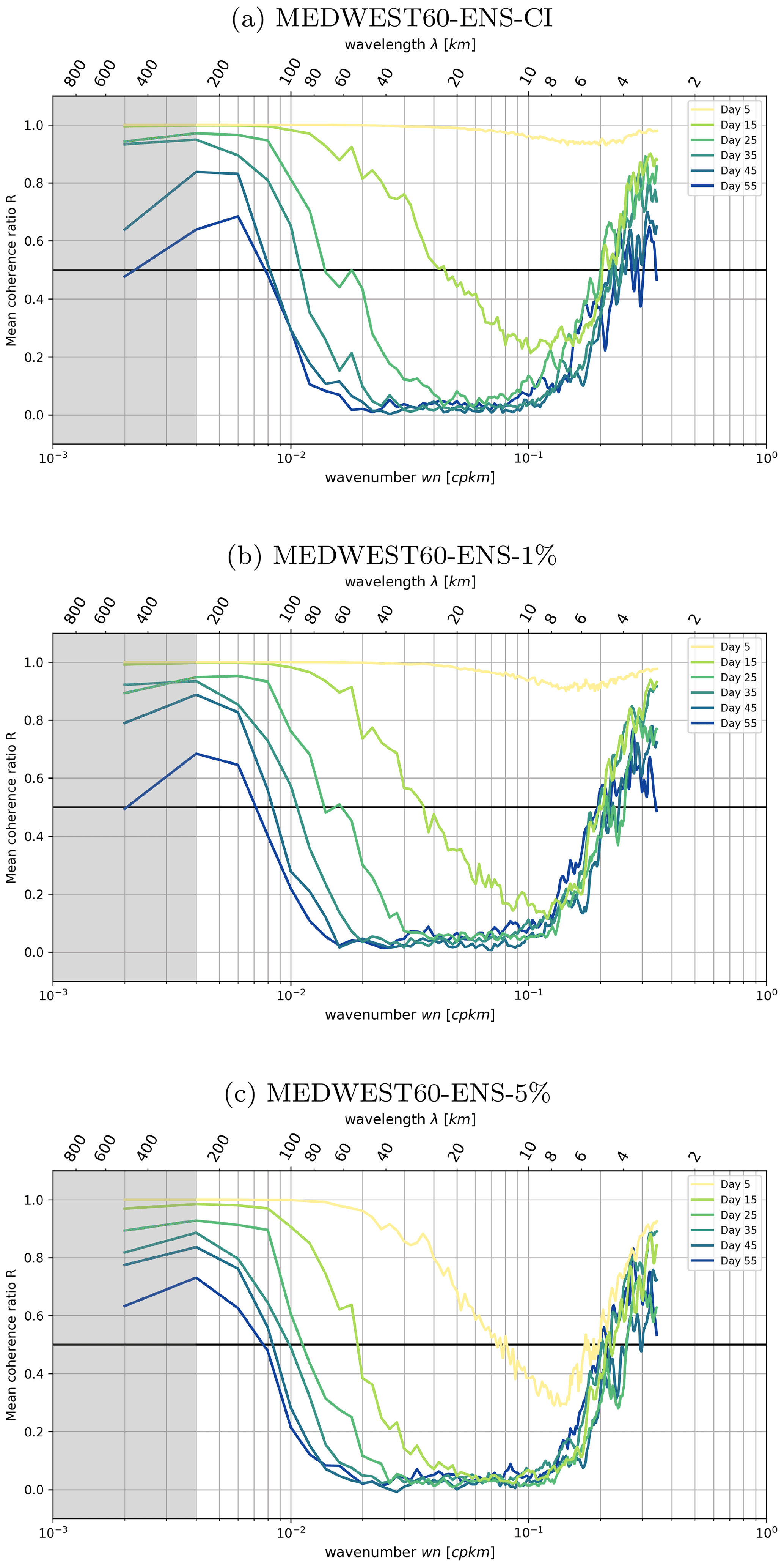
Figure 18Mean coherence ratio R (see text for definition) from experiments ENS-CI, ENS-1% and ENS-5%. The ratio is computed at different time lags: time increasing from yellow to blue colors. The gray shading indicates where the spatial scales are not fully resolved within the considered region (scales larger than km).
On the right side of the spectrum, on very small scales (<6 km), it is noteworthy that R remains larger than 0.5 after 2 months of simulation. This behavior is consistent in the three experiments (see panels a, b, c in Fig. 18), so it cannot just result from a spurious effect of the stochastic perturbation (which is not present in experiment ENS-CI). Specific investigations would be needed to understand better the reasons for this behavior, but note that it might just result from numerical noise (such as truncation errors, etc.), given the small amplitude of the signal (see Fig. 7) on the range of scales considered here (<6 km).
4.3.3 Evolution in time and predictability diagrams
To provide an example of a predictability diagram based on this spectral analysis, we finally consider the mean ratio , averaged over two given ranges of scales (10–30 and 60–100 km) from experiment ENS-CI in Fig. 19, following the same methodology as for the CRPS and location scores. The value of after a given forecast time lag, , where Δ is the time lag, is plotted as a function of the initial value . For each given scale range (panel a 10–30 km and panel b 60–100 km), the figure thus provides some objective information about the spatial decorrelation between the members (here in the case with no model uncertainty).
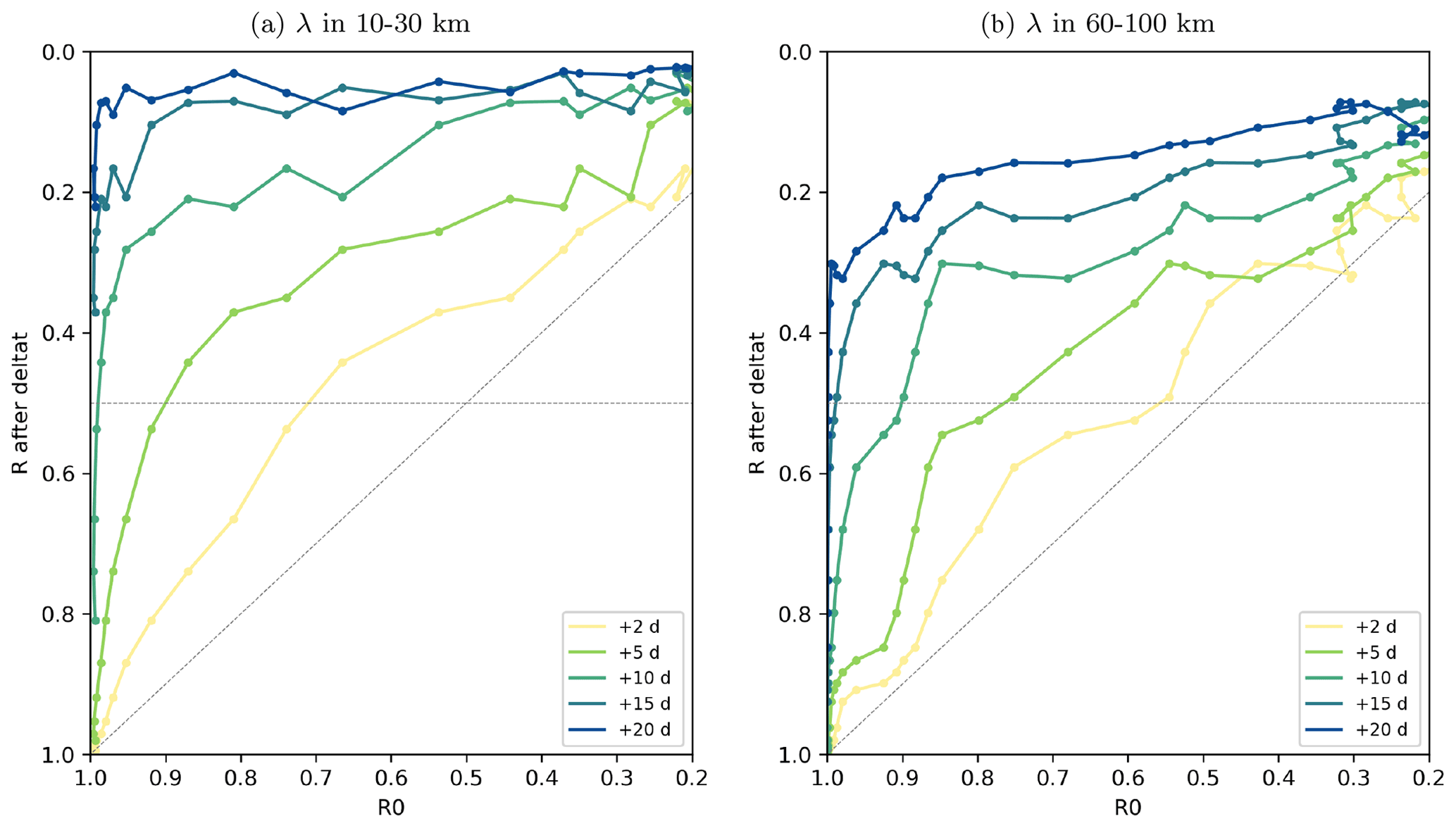
Figure 19Mean wavenumber spectral coherence ratio R of the ensemble forecast as a function of the coherence of the ensemble initial conditions, for different forecast time lags (+2, 5, 10, 15, 20 d), computed from hourly SSH in experiment ENS-CI. The mean ratio R is taken over scales of (a) 10–30 km and (b) 60–100 km. A gray horizontal line marks the value of the coherence ratio R at 0.5, at which we consider the decorrelation of the ensemble members as effective. The R0=Rforecast line is also marked in gray.
In the 10–30 km scale range for example, it appears that even with very small initial errors (initial R close to 1), the members become nearly decorrelated after a time lag of ∼10 d (i.e., ) on these scales. For the larger-scale range, 60–100 km, the threshold of is reached for time lags above ∼15 d. Note however that only the uncertainty in initial conditions is taken into account here. A faster decorrelation would be expected if other types of uncertainties in the forecast system were taken into account, such as uncertainty in the atmospheric forcing.
The kind of predictability diagrams proposed in Fig. 19 might also be relevant in the context of preparing for the assimilation of wide-swath high-resolution satellite altimetry such as expected from the future SWOT mission (Morrow et al., 2019). This mission is expected to measure sea surface height (SSH) with high precision and resolve short mesoscale structures as small as 15 km on a wide swath of 120 km. However the time interval between revisits will be within 11 to 22 d, depending on the location. Our results above tend to show that, for time lags longer than 10 d, the forecasting system considered in the present study will have lost most of the information in the initial condition regarding SSH structures in the smallest-scale range (10–30 km). With a perfect model and a very good assimilation system that would ensure an initial ratio R0 close to 1 (say 0.9 for the sake of the numerical application here) the spectral coherence ratio R of the forecast after 5 d drops down to 0.5 for scales in the range 10–30 km, while it remains above 0.8 for scales in the range 60–100 km at the same time lag. Or to put it differently, if the target for the spectral decorrelation was to remain above R=0.5 for all scales in the range 10–100 km, then a revisit time of the satellite between 5 and 10 d would be necessary (and even shorter with current imperfect models). This is why nadir altimeter data will remain a key component of the satellite constellation complementing the wide-swath SWOT measurements in space and time.
The general objective of this study was to propose an approach to quantify how much of the information in the initial condition a high-resolution NEMO modeling system is able to retain and propagate correctly during a short- and medium-range forecast.
For that purpose, a kilometric-scale, NEMO-based regional model for the Western Mediterranean (MEDWEST60, at ∘ horizontal resolution) has been developed. It has been defined as a subregion of a larger North Atlantic model (eNATL60), which provides the boundary conditions at an hourly frequency at the same resolution. This deterministic model has then been transformed into a probabilistic model by introducing an innovative stochastic parameterization of location uncertainties in the horizontal displacements of the fluid parcels. The purpose is primarily to generate an ensemble of initial conditions to be used in the predictability studies, and it has also been applied to assess the possible impact of irreducible model uncertainties on the accuracy of the forecast.
With this regional model, 20-member and 2-month ensemble experiments have been performed, first with the stochastic model for two levels of model uncertainty and then with the deterministic model from perturbed initial conditions. In all experiments, the spread of the ensemble emerges from the smallest model scales (i.e., kilometric) to progressively develop and cascade upscale to the largest structures. After 2 months, the ensemble variance has saturated over most of the spectrum (10–100 km) and the ensemble members have become decorrelated in this scale range. These ensemble simulations are thus appropriate to provide a statistical description of the dependence between initial accuracy and forecast accuracy over the full range of potentially useful forecast time lags (typically, between 1 and 20 d). Of course, the ensemble size can be a limitation of the accuracy of the conclusions. In our case, with N=20 members, we can expect a ∼16 % accuracy () in the ensemble standard deviation as an approximation to the true standard deviation, which is not perfect but sufficient to draw meaningful conclusions.
From these experiments, predictability has then been quantified statistically, using a cross-validation algorithm (i.e., using alternatively each ensemble member as a reference truth and the remaining 19 members as forecast ensemble) together with a few example scores to characterize the initial and forecast accuracy. From the joint distribution of initial and final scores, it was then possible to diagnose the probability distribution of the forecast score given the initial score, or reciprocally to derive conditions on the initial accuracy to obtain a target forecast accuracy. Although any specific score of practical significance could have been used, we focused here on simple and generic scores describing the misfit between ensemble members in terms of overall accuracy (CRPS score), geographical position of the ocean structures (location score) and spatial decorrelation.
Table 3Initial SST accuracy required (CRPS score, in ∘C) to obtain the target final accuracy (CRPS score, left column) with a 95 % confidence for different forecast time lags: 2, 5 and 10 d.
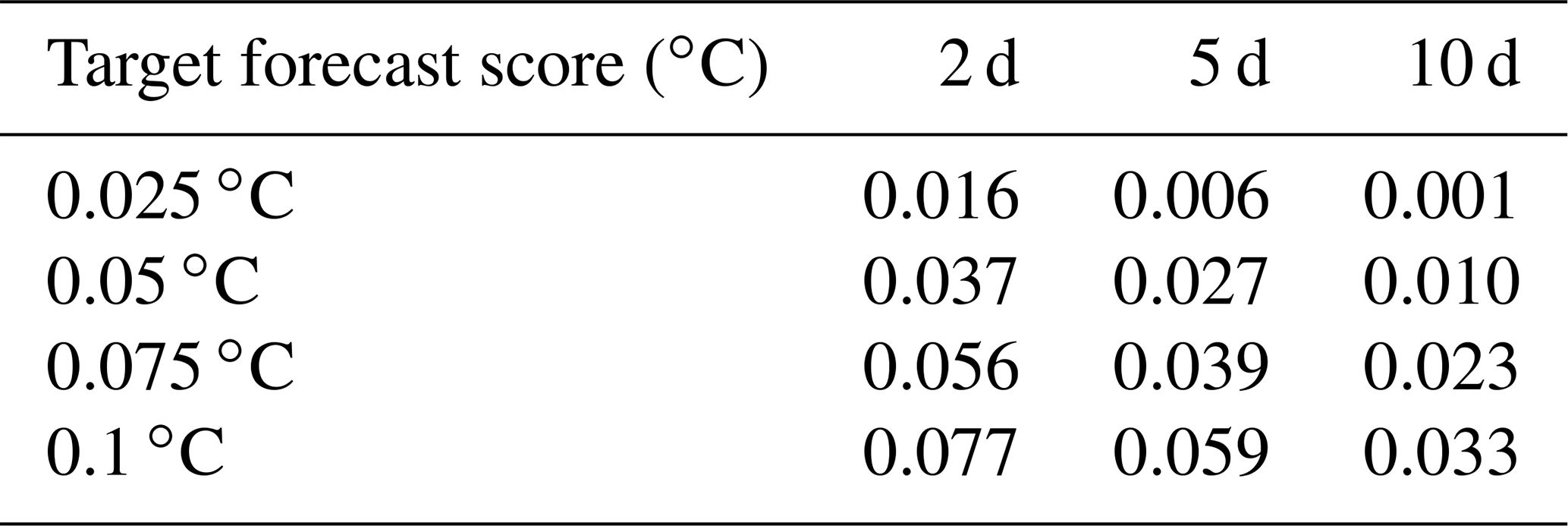
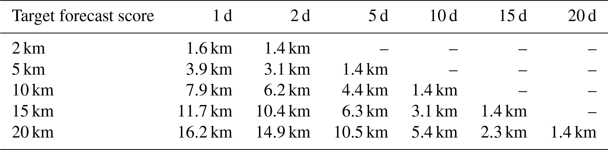
Tables 3 and 4 give a quantitative illustration of the conditions obtained on the initial accuracy to obtain a given forecast accuracy if the model is assumed to be perfect (as in experiment ENS-CI), using the CRPS score and the location score. For example, Table 4 shows that, for our particular region and period of interest, the initial location accuracy required with a perfect model (deterministic operator) to obtain a forecast location accuracy of 10 km with a 95 % confidence is about 8 km for a 1 d forecast, 6 km for a 2 d forecast, 4 km for a 5 d forecast and 1.5 km for a 10 d forecast and that this target is unreachable for a 15 and a 20 d forecast (more precisely, in these two cases, the required initial accuracy would be unrealistically small and was not included in our sample). With model uncertainties (stochastic operator, as in experiment ENS-1% or ENS-5%), the requirement on the initial condition can be even more stringent, especially for a short-range and high-accuracy forecast.
Table 4Initial location accuracy required (location score) to obtain the target final location accuracy (location score, left column) with a 95 % confidence for different forecast time lags between 1 d and 20 d.
However, it is important to remember that this only provides necessary conditions but not a sufficient conditions on the initial model state. The reason for this is that the condition is put on one single score for one single variable, whereas the quality of the forecast obviously depends on the accuracy of all variables in the model state vector. In the examples given in the tables, we used the same model variable for both target score and the condition score, but we could also have looked for a necessary condition on another variable (for instance velocity) to obtain a given forecast accuracy for SST or any other model diagnostic. In this way, for any forecast target, we could have accumulated many necessary conditions on various key properties of the initial conditions, especially observed properties, but this would never become a sufficient condition.
Furthermore, these necessary conditions on observed quantities can then be translated into conditions on the design of ocean observing systems, in terms of accuracy and resolution, if a given forecast accuracy is to be expected (e.g., on the wide-swath altimetry mission SWOT, as discussed in Sect. 4.3).
But, again, these conditions are only necessary conditions, as the accuracy of the initial model state also depends on the ability of the assimilation system to interpret properly the observed information and to produce an appropriate initial condition for the forecast. Checking this ability would have required performing observation system simulation experiments (OSSEs) using the operational assimilation system, which lay beyond the scope of the present work.
More generally, however, what this study suggests is that an ensemble forecasting framework should become an important component of operational systems to provide a systematic statistical quantification of the relation between the system operational target (a useful forecast accuracy) and the available assets: the observation systems, with their expected resolution and accuracy, and the modeling tools, with their target resolution and associated irreducible uncertainties.
The purpose of this appendix is to describe the stochastic parameterization that has been used in this paper to simulate model uncertainties in experiments ENS-1% and ENS-5%. Uncertainties are assumed to occur on the location of the fluid parcels as explained in Sect. A1. The further assumptions that are made to implement the resulting stochastic formulation in NEMO are presented in Sect. A2.
A1 Stochastic formulation
Location errors in a field φ(x,t), function of the spatial coordinates x and time t, occur if the field φ displays the correct values but not at the right location. More precisely, this means that the field φ(x,t) can be related to the true field φt(x,t) by the transformation:
where xt(x,t) is a transformation of the coordinates (anamorphosis) defining the location where to find the true value of φ(x,t). With respect to the true field φt, the values of φ are thus shifted by
which defines the location error.
If the field φ(x,t) is evolved in time, over one time step Δt, with the model ℳ,
we can make the assumption that one of the effects of the model is to generate location uncertainties. In an advection-dominated regime, this means for example that the displacement of the fluid parcels can be different from what the deterministic model predicts. With this assumption, the model transforms to
where the location error δx(x,t) can be simulated for instance by a stochastic process 𝒫:
where an explicit dependence on φ and t has been included here to keep the formulation general.
In ocean numerical models, the coordinates x are usually discretized on a constant grid. To implement the stochastic model of Eqs. (A4) and (A5) on this numerical grid, one possibility would be to remap the updated field on this constant grid at each model time step. This remapping would correspond to a stochastic shift in the model field accounting for the presence of location uncertainties. However, this solution may be computationally ineffective, and it is much easier to keep track of the modified location of the grid points (described by δx) and use this modified grid to implement the model operator ℳ. In practice, to avoid deteriorating the model numerics, this solution requires that location errors remain small with respect to the size of the grid cells and that their variations over one time step Δt are kept small enough to avoid undesirable numerical effects.
This simple approach to simulate location uncertainties in ocean models has a close similarity to the work of Mémin (2014) and Chapron et al. (2018), where it is argued that the effect of unresolved processes in a turbulent flow can be simulated by adding a random component to the Lagrangian displacement dX of the fluid parcels (as in a Brownian motion):
where v(x,t) is the velocity (as resolved by the model). σ(x,t)dB is a stochastic process uncorrelated in time but correlated in space, with a general formulation of the spatial correlation structure. σ(x,t) defines the amplitude and structure of the random displacement. The purpose of their study is then to examine the effect of this modified material derivative (with the stochastic displacement added) when transformed into an Eulerian framework (i.e., in a constant coordinate system). In a nutshell, from this assumption, the authors manage to derive modified Navier–Stokes equations, with additional deterministic and stochastic terms depending on σ.
A2 Implementation in NEMO
To implement location uncertainties in NEMO, we explicitly make the assumption that the location errors δx remain small with respect to the size of the grid cells, so that the nodes of the modified grid just follow a small random walk around the nodes of the original grid. Consistently with this assumption, we make the approximation that the model input data (bathymetry, atmospheric forcing, open-sea boundary conditions, river runoffs …) keep the same location with respect to the model grid, which means that these data are not remapped on the moving grid. Such a tiny shift in the data (much smaller than the grid resolution) would indeed represent a substantial computational burden, with many possible technical complications, and would only produce small additional perturbations to the model solution, which do not correspond to the main effect that we want to simulate.
Since the model grid is assumed to be fixed with respect to the outside world, we need only represent the displacement of each model grid point relative to its neighbors. In NEMO, this relative displacement of the model grid points can easily be obtained by transforming the metrics of the grid, which is numerically represented by the distance between the neighbor grid points. A stochastic metric, describing relative location uncertainties in the model operator ℳ, corresponds to the main effects that we want to simulate, because it can represent both physical and numerical uncertainties. On the one hand, the stochastic metric is an explicitly Lagrangian transcription of Eq. (A6) in the model dynamics, which describes physical uncertainties that upscale from unresolved processes. On the other hand, since the metrics is used everywhere in the model to evaluate differential and integral operators, making it stochastic can also be viewed as a simple approach to simulate numerical uncertainties simultaneously in all model components.
In practice, to obtain a stochastic metric in NEMO, we must transform the arrays describing the horizontal size of the grid cells into time-dependent stochastic processes. Thus, if is the size of grid cell number i at time t, we must define stochastic processes 𝒫i such that
A very simple approach to define 𝒫i is then to use first-order autoregressive processes ξi(t) as a multiplicative noise applied to the reference model grid :
with
where ∘ is the Hadamard product, w is a vector of independent Gaussian white noises, and a and b are constant coefficients governing the standard deviation and the correlation length scale of the ξi. The components of ξi are thus assumed to be independent, which means that the grid is deformed independently along the two horizontal dimensions.
The use of autoregressive processes ξi(t) to simulate the stochastic distortion of the model grid makes the implementation of the scheme straightforward in NEMO, since we can directly apply the tools developed by Brankart et al. (2015) to generate the ξi. This tool was indeed meant to be generic enough to trigger various sorts of stochastic parameterizations in NEMO and has already been used to simulate various sources of uncertainty, including the effect of unresolved scales in the seawater equation of state (Brankart, 2013; Bessières et al., 2017; Zanna et al., 2019) and in the biogeochemical equations (Garnier et al., 2016) or the effect of parameter uncertainties in the sea ice model (Brankart et al., 2015). This tool only requires specifying a few parameters to characterize the stochastic processes ξi(t): the standard deviation (σ), the correlation timescale (τ), the number of passes (P) of a Laplacian filter applied to the ξi and the order (n) of the autoregressive processes. The two last parameters go beyond the formulation of Eq. (A9), which describes first-order processes (AR1) uncorrelated in space. The application of a Laplacian filter (with a correction factor to restore the original standard deviation) introduces space correlation and makes the distortion of the grid smoother in space, and the use of ARn rather than AR1 processes modifies the time correlation structure and makes the distortion of the grid smoother in time. It must also be noted that the use of ARn processes is also more general than Eq. (A7) by making the processes 𝒫i depend on the n previous time steps rather than just the previous time step.
In the present study, the distortion of the grid has been limited to horizontal displacements of the model grid points, with the same displacements applied to all model fields and along the vertical. This reduces the number of stochastic fields to generate to two two-dimensional fields, one for each of the horizontal coordinates Δxi(t) and Δyi(t). However, since the NEMO fields are shifted according to the rules of the Arakawa C grid, the stochastic metric is first computed for the T grid and then transformed to the other grids (by linear interpolation) to be consistent with the shifted position of the grid points. In the application, the standard deviation is set to a relatively small value σ=1 % or 5 %, to be consistent with the assumption of small location errors, and the correlation timescale is set to 1080 time steps (1 d) to be consistent with the assumption of a small variation in the grid over one time step. Some effort is also made to keep the perturbation smooth in space and time by applying P=10 passes of a Laplacian filter and by using second-order autoregressive processes (n=2).
The source codes of the MEDWEST60 NEMO-based model and some of the diagnostics tools developed in this study are shared in an open GitHub repository dedicated to MEDWEST60 (release v1.0.1: https://doi.org/10.5281/zenodo.7220401, Leroux, 2022). The model outputs are available upon request (∼ 50 TB for the three ensemble simulations). The CDFTOOLS (https://github.com/meom-group/CDFTOOLS, Molines and the MEOM Group, 2022) were used for some of the pre- and post-processing of the model outputs. The power spectral density computations in Sects. 3.2 and 4.3 were all performed using Adekunle Ajayi's Python module PowerSpec (https://github.com/adeajayi-kunle/powerspec, Ajayi, 2022) and the predictability diagnostics based on CRPS score and location score were made with the SESAM (https://github.com/brankart/sesam, Brankart, 2022a) and EnsDAM (https://github.com/brankart/ensdam, Brankart, 2022b) software.
JLS, PB, TP and JMB proposed the initial model study. SL set up and ran the model with some assistance and instructive discussions with AA, LB, JMB, JMM and QJ. SL and JMB designed and applied the methodology to analyze the model outputs. SL and JMB wrote the initial paper and all authors commented on and contributed to draft revisions.
The contact author has declared that none of the authors has any competing interests.
Publisher’s note: Copernicus Publications remains neutral with regard to jurisdictional claims in published maps and institutional affiliations.
The work was performed using HPC resources from GENCI-IDRIS, France (grant A008-0101279).
This research has received funding from the European Union Horizon 2020 research and innovation program under grant agreement no. 821926 (H2020-IMMERSE, https://immerse-ocean.eu/, last access: 9 November 2022).
This paper was edited by Ismael Hernández-Carrasco and reviewed by two anonymous referees.
Ajayi, A.: PowerSpec, GitHub [code], https://github.com/adeajayi-kunle/powerspec, last access: 9 November 2022. a
Berner, J., Jung, T., and Palmer, T. N.: Systematic model error: the impact of increased horizontal resolution versus improved stochastic and deterministic parameterizations, J. Climate, 25, 4946–4962, https://doi.org/10.1175/JCLI-D-11-00297.1, 2012. a
Bessières, L., Leroux, S., Brankart, J.-M., Molines, J.-M., Moine, M.-P., Bouttier, P.-A., Penduff, T., Terray, L., Barnier, B., and Sérazin, G.: Development of a probabilistic ocean modelling system based on NEMO 3.5: application at eddying resolution, Geosci. Model Dev., 10, 1091–1106, https://doi.org/10.5194/gmd-10-1091-2017, 2017. a
Berloff, P. S. and McWilliams, J. C.: Material Transport in Oceanic Gyres. Part II: Hierarchy of Stochastic Models, J. Phys. Oceanogr., 32, 797–830, https://doi.org/10.1175/1520-0485(2002)032<0797:MTIOGP>2.0.CO;2, 2002. a
Brankart, J.-M.: Impact of uncertainties in the horizontal density gradient upon low resolution global ocean modelling, Ocean Model., 66, 64–76, https://doi.org/10.1016/j.ocemod.2013.02.004, 2013. a, b, c
Brankart, J.-M.: SESAM, GitHub [code], https://github.com/brankart/sesam, last access: 9 November 2022a. a
Brankart, J.-M.: EnsDAM, GitHub [code], https://github.com/brankart/ensdam, last access: 9 November 2022b. a
Brankart, J.-M., Candille, G., Garnier, F., Calone, C., Melet, A., Bouttier, P.-A., Brasseur, P., and Verron, J.: A generic approach to explicit simulation of uncertainty in the NEMO ocean model, Geosci. Model Dev., 8, 1285–1297, https://doi.org/10.5194/gmd-8-1285-2015, 2015. a, b, c
Brasseur, P., Blayo, E., and Verron, J.: Predictability experiments in the North Atlantic Ocean: Outcome of a quasi-geostrophic model with assimilation of TOPEX/POSEIDON altimeter data, J. Geophys. Res.-Oceans, 101, 14161–14173, https://doi.org/10.1029/96JC00665, 1996. a
Brodeau, L., Le Sommer, J., and Albert, A.: Ocean-next/eNATL60: Material describing the set-up and the assessment of NEMO-eNATL60 simulations (Version v1), Zenodo [code, data set], https://doi.org/10.5281/zenodo.4032732, 2020. a
Buizza, R., Miller, M., and Palmer, T. N.: Stochastic representation of model uncertainties in the ECMWF ensemble prediction system, Q. J. Roy. Meteor. Soc., 125, 2887–2908, https://doi.org/10.21957/db1w1xzch, 1999. a
Candille G. and Talagrand, O.: Evaluation of probabilistic prediction systems for a scalar variable, Q. J. Roy. Meteor. Soc., 131, 2131–2150, https://doi.org/10.1256/qj.04.71, 2005. a
Candille, G., Côté, C., Houtekamer, P. L., and Pellerin, G.: Verification of an ensemble prediction system against observations, Mon. Weather Rev., 135, 2688–2699, https://doi.org/10.1175/MWR3414.1, 2007. a
Candille, G., Brankart, J.-M., and Brasseur, P.: Assessment of an ensemble system that assimilates Jason-1/Envisat altimeter data in a probabilistic model of the North Atlantic ocean circulation, Ocean Sci., 11, 425–438, https://doi.org/10.5194/os-11-425-2015, 2015. a, b
Chapron B., Dérian, P., Mémin, E., and Resseguieri, V.: Large scale flows under location uncertainty: a consistent stochastic framework, Q. J. Roy. Meteor. Soc., 144, 251–260, https://doi.org/10.1002/qj.3198, 2018. a, b
Diaconescu, E. P. and Laprise, R.: Singular vectors in atmospheric sciences: A review, Earth-Sci. Rev., 113, 161–175, https://doi.org/10.1016/j.earscirev.2012.05.005, 2012. a
Escudier, R., Renault, L., Pascual, A., Brasseur, P., Chelton, D., and Beuvier, J.: Eddy properties in the Western Mediterranean Sea from satellite altimetry and a numerical simulation, J. Geophys. Res.-Oceans, 121, 3990–4006, https://doi.org/10.1002/2015JC011371, 2016. a
Evensen, G.: Sequential data assimilation with a non linear quasigeostrophic model using Monte Carlo methods to forecast error statistics, J. Geophys. Res., 99, 10143–10162, https://doi.org/10.1029/94JC00572,1994. a
Frederiksen, J., O'Kane, T., and Zidikheri, M.: Stochastic subgrid parameterizations for atmospheric and oceanic flows, Phys. Scripta, 85, 068202, https://doi.org/10.1088/0031-8949/85/06/068202, 2012. a
Garnier, F., Brankart, J.-M., Brasseur, P., and Cosme, E.: Stochastic parameterizations of biogeochemical uncertainties in a 1/4∘ NEMO/PISCES model for probabilistic comparisons with ocean color data, J. Marine Syst., 155, 59–72, https://doi.org/10.1016/j.jmarsys.2015.10.012, 2016. a
Germineaud, C., Brankart, J.-M., and Brasseur, P.: An Ensemble-Based Probabilistic Score Approach to Compare Observation Scenarios: An Application to Biogeochemical-Argo Deployments, J. Atmos. Ocean. Tech., 36, 2307–2326, https://doi.org/10.1175/JTECH-D-19-0002.1, 2019. a
Griffa, A.: Applications of stochastic particle models to oceanographic problems, in: Stochastic modelling in physical oceanography, edited by: Adler, R., Müller, P., and Rozovskii, B., Birkhuser Boston, 113–140, https://doi.org/10.1007/978-1-4612-2430-3_5, 1996. a
Hawkins, E., Smith, R. S., Gregory, J. M., and Stainforth, D. A.: Irreducible uncertainty in near-term climate projections, Clim. Dynam., 46, 3807–3819, https://doi.org/10.1007/s00382-015-2806-8, 2016. a
Hersbach, H.: Decomposition of the continuous ranked probability score for ensemble prediction systems, Weather Forecast., 15, 559–570, https://doi.org/10.1175/1520-0434(2000)015<0559:DOTCRP>2.0.CO;2, 2000. a
Juricke, S., Lemke, P., Timmermann, R., and Rackow, T.: Effects of stochastic ice strength perturbation on Arctic finite element sea ice modeling, J. Climate, 26, 3785–3802, https://doi.org/10.1175/JCLI-D-12-00388.1, 2013. a
Juricke, S., MacLeod, D., Weisheimer, A., Zanna, L., and Palmer, T. N.: Seasonal to annual ocean forecasting skill and the role of model and observational uncertainty, Q. J. Roy. Meteor. Soc., 144, 1947–1964, https://doi.org/10.1002/qj.3394, 2018. a
Kalnay, E.: Atmospheric Modeling, Data Assimilation and Predictability, Cambridge University Press, Cambridge, https://doi.org/10.1017/CBO9780511802270, 2003. a
Lacarra, J. and Talagrand, O.: Short-range evolution of small perturbations in a barotropic model, Tellus A, 40, 81–95, https://doi.org/10.1111/j.1600-0870.1988.tb00408.x, 1988. a
Lellouche, J.-M., Greiner, E., Bourdallé-Badie, R., Garric, G., Melet, A., Drévillon, M., Bricaud, M., Hamon, M., Le Galloudec, O., Regnier, C., Candela, T., Testut, C.-E., Gasparin, F., Ruggiero, G., Benkiran, M., Drillet, Y., and Le Traon, P.-Y.: The Copernicus Global 1/12 Oceanic and Sea Ice GLORYS12 Reanalysis, Front. Earth Sci., 9, 2296–6463, https://doi.org/10.3389/feart.2021.698876, 2021. a
Leroux, S.: ocean-next/MEDWEST60: v1.0.1 (v1.0.1), Zenodo [code], https://doi.org/10.5281/zenodo.7220401, 2022. a
Leutbecher, M., Lock, S., Ollinaho, P., Lang, S. T., Balsamo, G., Bechtold, P., Bonavita, M., Christensen, H. M., Diamantakis, M., Dutra, E., English, S., Fisher, M., Forbes, R. M., Goddard, J., Haiden, T., Hogan, R. J., Juricke, S., Lawrence, H., MacLeod, D., Magnusson, L., Malardel, S., Massart, S., Sandu, I., Smolarkiewicz, P. K., Subramanian, A., Vitart, F., Wedi, N., and Weisheimer, A.: Stochastic representations of model uncertainties at ECMWF: state of the art and future vision, Q. J. Roy. Meteor. Soc., 143, 2315–2339, https://doi.org/10.1002/qj.3094, 2017. a
Lorenz, E. N.: A study of the predictability of a 28-variable atmospheric model, Tellus, 17, 321–333, https://doi.org/10.1111/j.2153-3490.1965.tb01424.x, 1965. a
Lorenz, E. N.: Atmospheric predictability with a large numerical model, Tellus, 34, 505–513, https://doi.org/10.1111/j.2153-3490.1982.tb01839.x, 1982. a
Lorenz, E. N.: Predictability, a problem partly solved, Proceedings of Predictability ECMWF seminar, Seminar on Predictability, 4–8 September 1995, Shinfield Park, Reading, 1–18, https://www.ecmwf.int/en/elibrary/10829-predictability-problem-partly-solved (last access: 9 November 2022), 1995. a
Lyapunov, A.: The general problem of the stability of motion, Int. J. Control, 55, 531–534, https://doi.org/10.1080/00207179208934253, 1992. a
Lyard, F. H., Allain, D. J., Cancet, M., Carrère, L., and Picot, N.: FES2014 global ocean tide atlas: design and performance, Ocean Sci., 17, 615–649, https://doi.org/10.5194/os-17-615-2021, 2021. a
Madec, G. and NEMO System Team: NEMO ocean engine: Scientific Notes of Climate Modelling Center, Zenodo, https://doi.org/10.5281/zenodo.6334656, 2002. a
Mémin, E.: Fluid flow dynamics under location uncertainty, Geophys. Astro. Fluid, 108, 119–146, https://doi.org/10.1080/03091929.2013.836190, 2014. a, b
Molines J.-M. and the MEOM-IGE group: CDFTOOLS, GitHub [code], https://github.com/meom-group/CDFTOOLS, last access: 9 November 2022. a
Morrow, R., Fu, L.-L., Ardhuin, F., Benkiran, M., Chapron, B., Cosme, E., d'Ovidio, F., Farrar, J. T., Gille, S. T., Lapeyre, G., Le Traon, P.-Y., Pascual, A., Ponte, A., Qiu, B., Rascle, N., Ubelmann, C., Wang, J., and Zaron, E. D.: Global Observations of Fine-Scale Ocean Surface Topography With the Surface Water and Ocean Topography (SWOT) Mission, Frontiers in Marine Science, 6, 232, https://doi.org/10.3389/fmars.2019.00232, 2019. a
Palmer, T. and Hagedorn, R. (Eds.): Predictability of weather and climate, Cambridge University Press, https://doi.org/10.1017/CBO9780511617652, 2006. a
Palmer, T., Shutts, G., Hagedorn, R., Doblas-Reyes, F., Jung, T., and Leutbecher, M.: Representing model uncertainty in weather and climate prediction, Annu. Rev. Earth Pl. Sc., 33, 163–193, https://doi.org/10.1146/annurev.earth.33.092203.122552, 2005. a
Palmer, T. N.: The economic value of ensemble forecasts as a tool for risk assessment: From days to decades, Q. J. Roy. Meteor. Soc., 128, 747–774, https://doi.org/10.1256/0035900021643593, 2002. a
Robinson, A. R., Haley, P. J., Lermusiaux, P. F. J., and Leslie, W. G.: Predictive Skill, Predictive Capability and Predictability in Ocean Forecasting, Proceedings of “The OCEANS 2002 MTS/IEEE” conference, Holland Publications, 787–794, https://doi.org/10.1109/OCEANS.2002.1192070, 2002. a
Sakov, P., Counillon, F., Bertino, L., Lisæter, K. A., Oke, P. R., and Korablev, A.: TOPAZ4: an ocean-sea ice data assimilation system for the North Atlantic and Arctic, Ocean Sci., 8, 633–656, https://doi.org/10.5194/os-8-633-2012, 2012. a
Toth, Z. and Kalnay, E.: Ensemble Forecasting at NMC: The Generation of Perturbations, B. Am. Meteorol. Soc., 74, 2317–2330, https://doi.org/10.1175/1520-0477(1993)074<2317:EFANTG>2.0.CO;2, 1993. a
Williams, P. D., Howe, N. J., Gregory, J. M., Smith, R. S., and Joshi, M. M.: Improved climate simulations through a stochastic parametrization of ocean eddies, J. Climate, 29, 8763–8781, https://doi.org/10.1175/JCLI-D-15-0746.1, 2016. a
Ying, Y. K., Maddison, J. R., and Vanneste, J.: Bayesian inference of ocean diffusivity from Lagrangian trajectory data, Ocean Model., 140, 101401, https://doi.org/10.1016/j.ocemod.2019.101401, 2019. a
Zanna, L., Brankart, J.-M., Huber, M., Leroux, S., Penduff, T., and Williams, P. D.: Uncertainty and Scale Interactions in Ocean Ensembles: From Seasonal Forecasts to Multi-Decadal Climate Predictions, Q. J. Roy. Meteor. Soc., 145, 160–175, https://doi.org/10.1002/qj.3397, 2019. a
- Abstract
- Introduction
- A kilometric-scale regional ocean model
- A set of three ensemble forecast experiments
- Predictability diagnostics
- Summary and conclusions
- Appendix A: Location uncertainties
- Code and data availability
- Author contributions
- Competing interests
- Disclaimer
- Acknowledgements
- Financial support
- Review statement
- References