the Creative Commons Attribution 4.0 License.
the Creative Commons Attribution 4.0 License.
 | 13 Oct 2022
A clustering approach to determine biophysical provinces and physical drivers of productivity dynamics in a complex coastal sea
Elise M. Olson
Susan E. Allen
Debby Ianson
Karyn D. Suchy
The balance between ocean mixing and stratification influences primary productivity through light limitation and nutrient supply in the euphotic ocean. Here, we apply a hierarchical clustering algorithm (Ward's method) to four factors relating to stratification (wind energy, freshwater index, water-column-averaged vertical eddy diffusivity, and halocline depth), as well as to depth-integrated phytoplankton biomass, extracted from a biophysical ocean model of the Salish Sea. Running the clustering algorithm on 4 years of model output, we identify distinct regions of the model domain that exhibit contrasting wind and freshwater input dynamics, as well as regions of varying water-column-averaged vertical eddy diffusivity and halocline depth regimes. The spatial regionalizations in physical variables are similar in all 4 analyzed years. We also find distinct interannually consistent biological zones. In the northern Strait of Georgia and Juan de Fuca Strait, a deeper winter halocline and episodic summer mixing coincide with higher summer diatom abundance, while in the Fraser River stratified central Strait of Georgia, shallower haloclines and stronger summer stratification coincide with summer flagellate abundance. Cluster-based model results and evaluation suggest that the Juan de Fuca Strait supports more biomass than previously thought. Our approach elucidates probable physical mechanisms controlling phytoplankton abundance and composition. It also demonstrates a simple, powerful technique for finding structure in large datasets and determining boundaries of biophysical provinces.
- Article
(13712 KB) - Full-text XML
- BibTeX
- EndNote


Marine phytoplankton form the basis of the oceanographic food web and are responsible for approximately half of global carbon fixation (Field et al., 1998). To predict changes in global ecosystem functioning, it is necessary to understand the underlying controls on marine productivity. Primary productivity in the near-surface ocean is controlled by the availability of macronutrients, micronutrients, and light, as well as temperature, which are in turn controlled by the interplay of stratifying processes and sources of mixing.
The breakdown of the surface ocean stratified layer may reduce the availability of light for phytoplankton, inhibiting growth (e.g., Sverdrup, 1953), or contrastingly bring nutrients from deeper waters to nutrient-depleted surface waters, thus stimulating growth. The interplay of different stratification regimes exerts control on the structure of ocean ecosystems (e.g., Legendre, 1981), and changes in regime have been linked to shifts in phytoplankton community composition (e.g., Huisman et al., 2004).
The importance of phytoplankton in biogeochemical cycling, as well as their position at the base of the food web and impact on higher trophic levels, globally motivates the study of phytoplankton distribution and dynamics. Coastal regions are more productive than the open ocean (e.g., Longhurst et al., 1995). Simultaneously, these regions typically have more complex mixing, circulation, and stratification dynamics than the open ocean, making resolution of phytoplankton biomass patterns difficult. Finally, because both ocean stratification patterns and phytoplankton biomass dynamics may be expected to shift under anthropogenic climate change (Richardson, 2008), there is a need to characterize their dynamic structure and identify key drivers.
1.1 Oceanographic setting
The Salish Sea is a semi-enclosed fjord-like estuary on the British Columbia coast, composed of the Strait of Georgia (SoG), Juan de Fuca Strait (JdF), and Puget Sound (Fig. 1). The SoG is connected to the open ocean by Juan de Fuca Strait to the south and Johnstone Strait to the north, with Juan de Fuca Strait serving as the site of primary seawater exchange with the open ocean (Khangaonkar et al., 2017). The Salish Sea receives freshwater input from over 200 rivers, but the primary freshwater source is the nival–glacial Fraser River (Pike et al., 2010), which drives salinity-induced stratification in the CSoG and a strong estuarine exchange (Giddings and MacCready, 2017). Salinity stratification is opposed by wind and tidal action. Strong winds in the fall and winter months lead to mixing of surface and intermediate water masses. The SoG contains two deep basins (north and central), with the Fraser River plume sitting on top of the central basin. Deep SoG water is relatively unmixed, except during deep-water renewal events (Masson, 2002).
This coastal ocean is a region of ecological and cultural importance, providing habitats for important megafauna, including the southern resident killer whales (Orcinus orca) and the local salmon populations. The ongoing significant decline of the local Coho and Chinook salmon (Preikshot et al., 2013) has been implicated as a factor in the low reproductive success of the killer whale populations (Wasser et al., 2017), which depend on these salmon as a food source. The health of fish populations in the Pacific Northwest has been linked to spring bloom timing and phytoplankton abundance (e.g., Malick et al., 2015; Boldt et al., 2019). Thus, potential population declines in upper trophic levels further motivate the understanding of factors controlling the base of the food web.
The physical environment of the Salish Sea is well-known, with functionally distinct physical–oceanographic regions (Thomson, 1981; LeBlond, 1983; Pawlowicz et al., 2020). An ongoing subject of interest in this coastal sea is the relationship between known physical and presumed ecological regions. Three prominent parts of the Salish Sea–Juan de Fuca Strait (JdF), the northern Strait of Georgia (NSoG), and the central SoG (CSoG) have been defined by distinct stratification regimes and water mass characteristics, and available biological observations and model results (e.g., Masson and Peña, 2009; Suchy et al., 2019; Peña et al., 2016) are typically discussed in the context of these differing physical environments. However, in situ sampling of phytoplankton biomass remains relatively sparse and episodic and may not capture inherently dynamic phytoplankton biomass fluctuations, and remote sensing approaches can provide only surface chlorophyll concentrations. Here, we aim to use an unsupervised cluster analysis of a well-resolved sub-mesoscale mechanistic biophysical model to consider the linkages between the regional physical oceanography of the system and its phytoplankton biomass dynamics.
1.2 Application of clustering methods to a modeling framework
Clustering methods have demonstrated utility in identifying underlying structures in large observational datasets and are commonly used in ecological and biological observational studies. In recent years, the application of clustering to physical and biogeochemical ocean models has become more common (e.g., Sonnewald et al., 2020; Follows et al., 2007; Sun et al., 2021), though these approaches are not yet in widespread use. The quantity of data motivates the use of clustering methods in a modeling context – even in our relatively spatially limited sub-mesoscale resolution model, 1 year of output of a single variable at hourly resolution is quite sizable (∼ 60 GB and ∼ 3×10¹⁰ individual values); the output of global circulation models is considerably larger. Well-tuned, high-resolution numerical models of complex natural systems are uniquely poised to provide insight regarding physical oceanographic regimes and overarching patterns, especially in diverse regimes where sampling efforts are sparse and often seasonally biased to fair weather. However, interpreting (even visualizing) large volumes of data poses a unique challenge; common approaches, such as monthly averaged map snapshots, may represent an oversimplification and fail to show the patterns present in the underlying system. By extracting small-data key metrics throughout the model domain, we reduce the size of the problem we are considering while keeping the key characteristics of the system that we are studying. We can then cluster these metrics in the hopes of revealing discrete dynamical regimes in complex regions. Furthermore, the clustering method is an objective classification of the system in the sense that it makes no prior assumptions about the locations of any oceanographic features that it finds.
Here our main goal is to investigate how physical dynamics in the Salish Sea objectively define regions of distinct phytoplankton biomass and functional group composition. We extract model-available proxies for four separate factors related to water column stratification: wind energy, freshwater index, water-column-averaged vertical eddy diffusivity, and halocline depth, as well as one indicator of primary productivity (depth-integrated phytoplankton biomass separated by functional group). We then cluster each factor individually in order to discuss the three major regions of the Salish Sea in the context of the spatial patterns in the yearly signals of these factors, as well as to consider their interannual variability. We finally compare spatial patterns in stratification factors to spatial patterns in phytoplankton biomass and discuss possible linkages between the two.
2.1 The SalishSeaCast biophysical model
We use SalishSeaCast, a regional oceanographic model developed for the Salish Sea (Soontiens et al., 2016; Soontiens and Allen, 2017) using version 3.6 of the NEMO regional ocean modeling engine (Madec et al., 2017). The physical model solves the Reynolds-averaged Navier–Stokes equations on an Arakawa-C grid with a 2 s barotropic time step, a 2 s vertical advection time step, and a 40 s baroclinic time step. Major physical model modifications since the first implementation are summarized in Olson et al. (2020).
The model domain (Fig. 1) is 898 (v) by 398 (u) horizontal cells with approximately 500 m horizontal resolution and 40 vertical z layers ranging from 1 m resolution at the surface to 27 m resolution at the bottom. SalishSeaCast has two open boundaries at JdF and Johnstone Strait, which are forced with eight tidal constituents and sea surface height predictions from NOAA's storm surge forecast at Neah Bay in JdF near the seaward entrance. The model is forced with over 150 rivers; the Fraser River runoff is taken from the Environment and Climate Change Canada flow gauge at Hope, BC, and the remaining rivers, as well as the Fraser River downstream of Hope, are forced by a monthly climatology (Morrison et al., 2012). Atmospheric forcing, including winds and solar radiation, is derived from the High Resolution Deterministic Prediction System (HRDPS), a nested 2.5 km resolution operational atmospheric model (Milbrandt et al., 2016). The HRDPS model output is too coarse to accurately resolve atmospheric conditions in the northern inlets, but its wind fields have shown good agreement with observations throughout the Strait of Georgia (Moore-Maley and Allen, 2022). Coupled to the physical model is a NPZD-type biological model (SMELT – Salish Sea Lower Trophic Ecosystem Model; Olson et al., 2020), which is described in summary below.
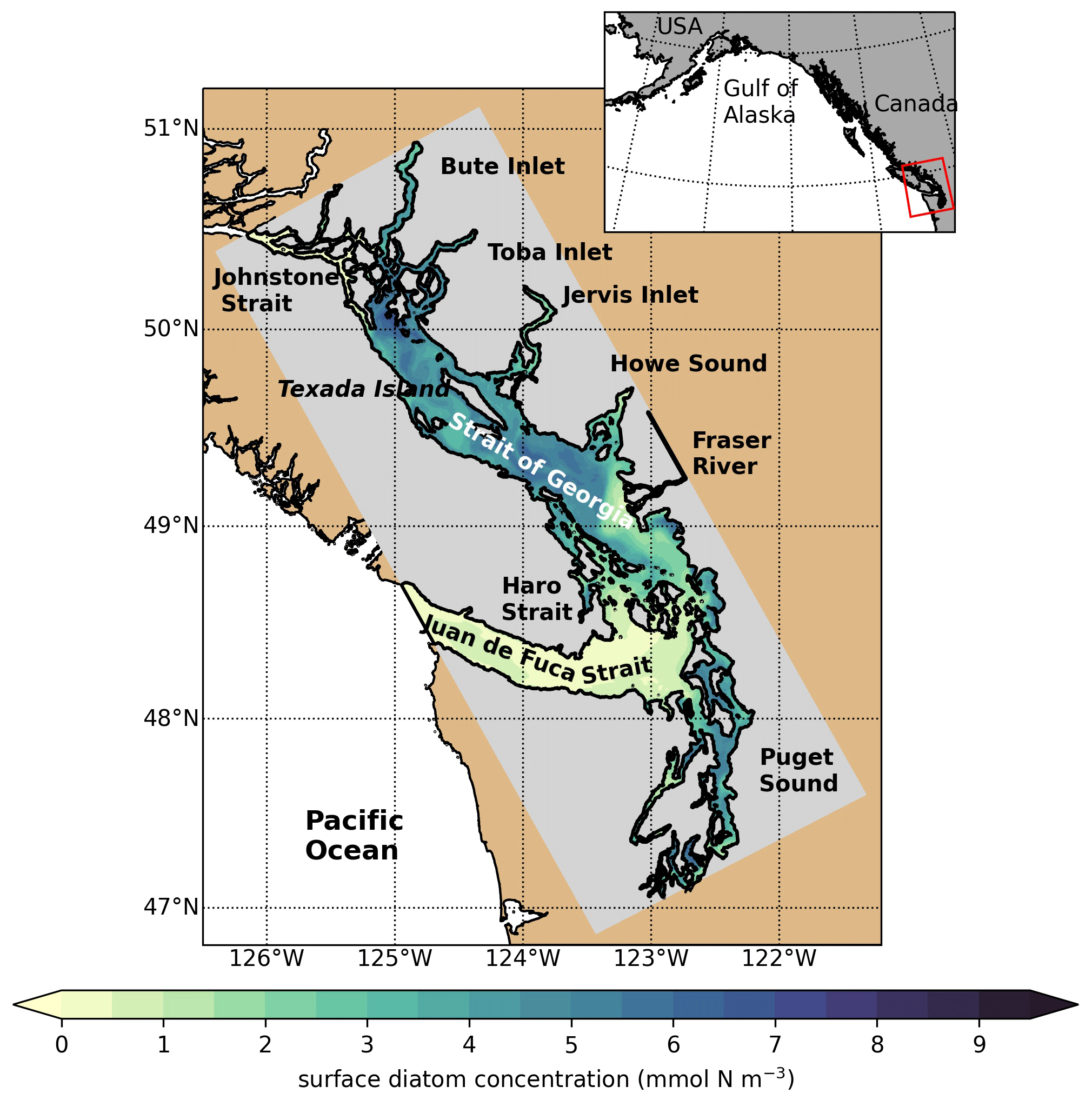
Figure 1SalishSeaCast model domain colored by 1 d of surface diatom concentration (1 April 2016), highlighting major geographic subregions and features. The Strait of Georgia is often subdivided into the central Strait of Georgia (CSoG) and northern Strait of Georgia (NSoG), with the divide between the two subregions occurring approximately near the southern tip of Texada Island.
The SMELT biological model represents the transfer of matter, using nitrogen as currency, between three classes of primary producers (diatoms, small flagellates, and the ciliate mixotroph M. rubrum), three classes of nutrients (nitrate, ammonia, and silicic acid), three classes of detritus (particulate and dissolved organic nitrogen, and biogenic silica), and one class of microzooplankton, with mesozooplankton grazing as a closure term. The growth rate of all three primary producer classes depends on the availability of nutrients and light and on temperature. The diatom class is assigned the highest maximum growth rate and the highest optimal light level and is the only class to take up dissolved silica – in the gleaner–opportunist framework, we consider it an opportunist class (Grover, 1990; Grover et al., 1997). Small flagellates (representing phytoplankton groups such as cryptophytes) have the lowest maximum growth rate while competing better at low nitrogen levels, low light, and higher temperature. Small flagellates have the lowest minimum nutrient requirement, and we consider them the gleaner class in the gleaner–opportunist framework. The mixotroph M. rubrum has intermediate growth parameters while grazing on the flagellate class in addition to photosynthesizing. Details of phytoplankton growth rate as well as nutrient and light level preference are available in Olson et al. (2020). A summary of minor updates to the model tuning since publication in Olson et al. (2020) is provided in Appendix B.
SalishSeaCast has been run operationally since 2014, and results from a 2013 to 2021 hindcast are available at https://salishsea.eos.ubc.ca/erddap/index.html (last access: 10 May 2022). The entire model system, including run environment, is documented at https://salishsea-meopar-docs.readthedocs.io (last access: 10 May 2022). In Appendix A we provide an evaluation of the model salinity, temperature, nitrate, dissolved silica, and chlorophyll against available observations for the years and model version analyzed, separated according to the major clusters found (Figs. A1–A2). In summary, the model shows consistently high skill across all clusters (Tables A1–A2), with Willmott skill scores for temperature and salinity ranging from 0.957–0.971 and 0.959–0.971, respectively, while comparisons with log-transformed total chlorophyll data yield scores of 0.599–0.712.
2.2 Stations and clustering signals
We analyzed 4 years of daily output from a hindcast of SalishSeaCast (2013–2016) using an unsupervised clustering algorithm (Ward's Euclidean distance method, see Sect. 2.3). We developed model-available year-long time series proxies (“signals”) for four different factors relating to stratification and mixing activity (wind strength, freshwater influx, vertical eddy diffusivity, and halocline depth) and one for an indicator of biological productivity (total depth-integrated biomass of three phytoplankton functional groups from the model's NPZD module). These signals were extracted for each year at each of 571 model “stations” spaced 10 model grid points apart (∼ 5 km, Fig. 2). This spacing was chosen as a compromise between resolution and computing time, and we believe it represents the different regions of the Salish Sea well while being computationally manageable.
Several possible clusterings resulting from our analysis were visualized and compared for major differences (see Sect. 2.3). Results show the typical cluster structure for all 4 years for each individual factor (Sect. 3), while an example visualization of all possible clusterings of 1 year of one of the variables is available in Fig. C1 in Appendix C. Here, we describe the signals.

Figure 2Example yearly signals of clustered physical and biological factors from one station in the CSoG (red star) for the year 2014. The physical signals are as follows: (a) wind energy (m3 s−3), (b) water-column-averaged vertical eddy diffusivity (m2 s−1), (c) freshwater index (g kg−1), (d) halocline depth (m). The biological signal is water-column-integrated phytoplankton biomass (mmol N m−2) separated by functional group (diatoms, ciliates, and flagellates). The remaining 570 stations used in the clustering are shown as blue points. Depth-integrated phytoplankton biomass signals are combined in series for clustering (see Fig. 8).
2.2.1 Wind strength
The wind forcing used (HRDPS, see model description) has 2.5 km spatial resolution and hourly temporal resolution, and it is used operationally by Environment Canada in the Canadian Pacific region. The skill of the HRDPS wind product in this region when compared to local meteorological stations has been evaluated by a previous study and accurately reproduces the climatology of observed wind magnitudes and directions (Moore-Maley and Allen, 2022). We first interpolate this product onto the model grid and then extract hourly wind speed. Here we are interested in the impact of wind on mixing of the water column. Therefore, because wind energy available for mixing scales with the cube of wind speed (Fischer et al., 1979), we use the cube of wind speed as our signal. To take advantage of the hourly resolution of the wind product, we use the daily average of cubed hourly wind speed (Fig. 2a).
2.2.2 Vertical eddy diffusivity
The vertical eddy diffusivity (VED) represents the strength of mixing in the system (Soontiens and Allen, 2017) and depends on the choice of vertical turbulence closure scheme. SalishSeaCast uses a k-ϵ configuration of a generic length scale turbulence model to estimate sub-grid-scale turbulent processes (Umlauf and Burchard, 2003), with background vertical eddy viscosity and diffusivity both set to 10−6 m2 s−1. We report a daily depth-averaged value (Fig. 2b). Though average vertical eddy diffusivity reflects all sources of mixing and stratification present in the system, it is dominated by barotropic tidal activity, and we expect it to be highest at tidal mixing hotspots (Crean, 1978).
2.2.3 Freshwater index
The freshwater index (Fig. 2c) is intended as a proxy for freshwater influence on the water column at a given station and is expressed as the salinity difference between the mean of the surface 4 m of the water column and the salinity at depth 50 m (units: g kg−1). This metric may be thought of as a salinity stratification metric. Where the water column is shallower than 50 m, the salinity at 50 m at the nearest model point that is 50 m deep is used. Similar metrics have been used as indicators of stratification in the region (Suchy et al., 2019; Masson and Peña, 2009) but were typically based on the difference in water density between the surface and the deep waters; here we isolate the impact of salinity alone by using a salinity-based metric. As salinity dominates stratification in this region (LeBlond, 1983), we expect clusters derived from a salinity-based clustering to be broadly similar to those derived from a density-based clustering. The value of 50 m was chosen because the majority of the Salish Sea is more than 50 m deep; however, we do not expect the results to change dramatically if a different depth were to be chosen.
2.2.4 Halocline depth
The halocline depth (Fig. 2d) is defined as the depth of the maximum salinity gradient in the water column, which is estimated by finding the salinity difference of two adjacent cells in the vertical dimension and reporting the depth at the midpoint of the two cells that have the maximum salinity gradient in the water column at a given station.
2.2.5 Phytoplankton biomass
We extract daily average depth-integrated phytoplankton biomass (mmol N m−2) for each of the three phytoplankton functional groups to form three signals (Fig. 2e). These signals are then connected in series to form an overall phytoplankton biomass signal that differentiates by functional group – thus, functional group identity, not just total phytoplankton biomass, is a factor in our clustering. Furthermore, our chosen metric of functional-group-differentiated phytoplankton biomass will capture functional-group-specific responses to different habitat characteristics.
2.3 Clustering method
We use Ward's method (Ward, 1963), a type of hierarchical clustering method, to cluster our data. Broadly, clustering methods are a subset of unsupervised machine learning methods used to reveal the underlying structure of a dataset by grouping similar data points. In hierarchical clustering methods, every data point is initially a single-point data cluster. At each step of the clustering, the two “closest” clusters are merged into a new cluster; this process is repeated until all points have been merged into a single cluster. Metrics of closeness vary between hierarchical clustering methods – while some methods use variations of the definition of the physical distance between clusters as a clustering criterion, Ward's method analyzes changing intracluster variance, or the “loss of information” (Wishart, 1969) if they were to merge into a single cluster. In Ward's method, at each step, the clusters whose merging results in the lowest increase in intracluster variance are combined.
Many hierarchical clustering methods exist; of these we chose Ward's method because the algorithm is straightforward to implement and compares favorably to other hierarchical clustering methods with regards to performance in identifying structure in known clusterings (e.g., Mangiameli et al., 1996). We perform hierarchical clustering using Ward's method on each of the five signals independently. For each signal, the clustering is done four times (once for each of the 4 years 2013–2016), and the results for the 4 years are then compared to assess interannual variability in the patterns found.
Cluster number selection
A common challenge in the application of clustering methods is the selection of cluster number, as the clustering algorithm can produce anywhere between two and N clusters (where N is the number of stations with signals being clustered). Typical approaches include choosing a cluster number for which the difference in the mean signals of the found clusters when going from cluster number N to cluster number N+1 is maximized. In our case, attempts to use objective metrics to determine cluster number, such as the Davies–Bouldin, silhouette, or Calinski–Harabasz criteria (Maulik and Bandyopadhyay, 2002), typically identified only two clusters in a given dataset (not shown). Though these may be the most prominent clusters, meaningful structure in the data persists at larger cluster numbers. Ultimately, our approach was to visualize several possible clustering outputs, with cluster number N varying from 2 to 15, and to visually compare how the spatial structure of the patterns changed with increasing cluster number (e.g., Fig. C1). In all variables, the same typical structure emerged at a relatively low cluster number (e.g., N = 3–5) and persisted with increasing cluster number in all years. To facilitate comparison of clusters between years, we chose a cluster number of N=5 for all years for all variables being clustered and are confident that the structures described are robust to a selection of a variety of cluster numbers.
Interannual cluster persistence
Visually, it is immediately apparent that similar spatial structure in the clusterings of a single variable persists interannually. To formalize the interannual persistence of a single cluster between years, as well as spatial commonality of different variables, we establish a simple nondimensional cluster commonality metric (CC). For two clusters A and B, the cluster commonality CCAB is defined as
For any two clusters, CC varies from 0 (clusters of any size with no stations in common) to 1 (two clusters of equal size with all stations in common) and may be used to compare clusters of unequal sizes. We use this metric to compare the persistence of clusters of individual variables between years, as well as the cluster persistence between different variables in a given year (Fig. C2).
We describe the main physical–oceanographic subregions in the domain (CSog, NSoG, and JdF) determined by clustering the physical factors and interpret our results in the context of previous work. We also consider some tidal mixing hotspots highlighted in the derived map of vertical eddy diffusivity. Our results here typically extract the main known general physical–oceanographic features of this coastal sea. We then describe the observed spatial regions in biomass, which are remarkably cohesive, in the context of these physical factors. In the Discussion section, we propose some mechanisms through which the physical factors likely shape the biological structures seen here.
3.1 Central Strait of Georgia
The physical–oceanographic dynamics of the CSoG are dominated by stratification due to Fraser River runoff, which is easily visible in the derived clustering of the freshwater index (Fig. 3). Spatially, in all 4 years of our analysis, the highest freshwater index is seen near the mouth of the Fraser River and in Howe Sound (cluster 1/gold), and it then radially decreases in bands (cluster 2/grey, cluster 3/sky blue) outward from this maximum. The tendency of the surface Fraser River plume to move north from the mouth of the Fraser due to the Coriolis force (Liu, 2014) is also easily observable in this visualization. The stratifying tendency of the Fraser River (and of other major rivers) is then reflected in the clustering of the halocline signals (Fig. 4). The CSoG (cluster 3/sky blue) has consistently shallow haloclines with only limited seasonal variability (∼ 5 m in summer to ∼ 7 m in winter). These shallow, stable haloclines also persist in most of the Puget Sound, owing to the influence of the Skagit River, and in the northern fjords with large rivers at their head (Toba Inlet, Bute Inlet, and Howe Sound), and the influence of these rivers is reflected in the clustering of the freshwater index. Because rivers other than the Fraser are forced by climatology in the model, the potential effects of the interannual variability of their hydrographs are not seen here.
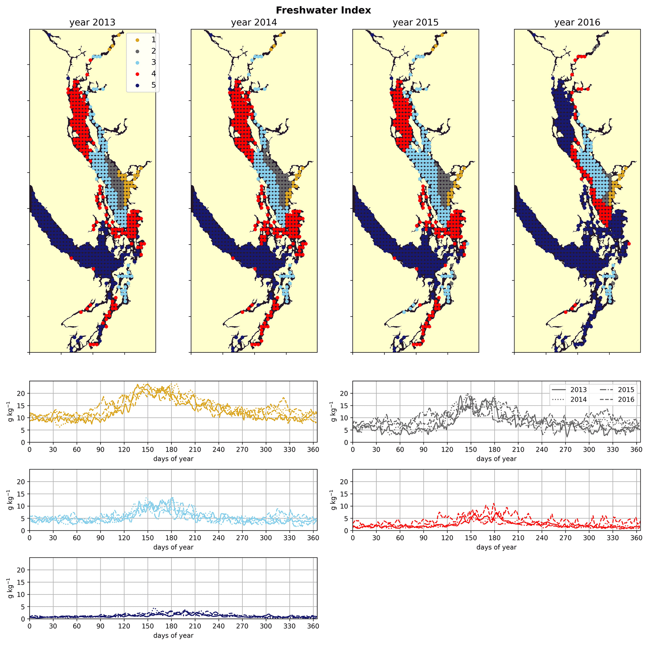
Figure 3Clustering of the freshwater index signal (Sect. 2.2). As expected, areas near the mouth of the Fraser River have the highest freshwater index, with the freshwater plume turning north due to the Coriolis force, and the index decreases in bands from this maximum. An elevated freshwater index can also be seen in the vicinity of the Skagit River in Puget Sound and at the head of Toba Inlet, Bute Inlet, and Howe Sound, which contain glacial rivers. The magnitude of the freshwater index in the different clusters does not vary significantly interannually, but the spatial extent is diminished in the year 2016, which had the lowest freshet magnitude of the 4 years. In all clusters, the freshwater index peaks at the same time as the Fraser freshet does for a given year.
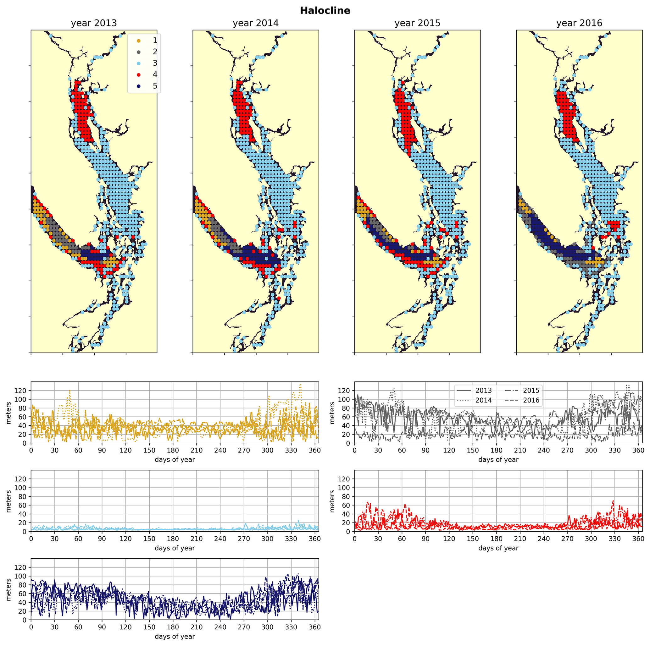
Figure 4Clustering of the halocline signal, defined as the depth of the maximum salinity gradient. The largest region (cluster 3, light blue) is the freshwater influenced CSoG, with shallow (<10 m) haloclines and limited variability between seasons. Similar halocline dynamics are seen in Puget Sound and at the head of Toba Inlet, Bute Inlet, and Howe Sound, which contain glacial rivers. Significantly deeper and more variable haloclines are found in the NSoG (cluster 4, red), commonly deeper than 40 m in winter. The deepest and most spatially variable haloclines occur in the center of the JdF (clusters 1, 2, and 5), with nearshore regions of the JdF clustering with the NSoG in most years (cluster 4).
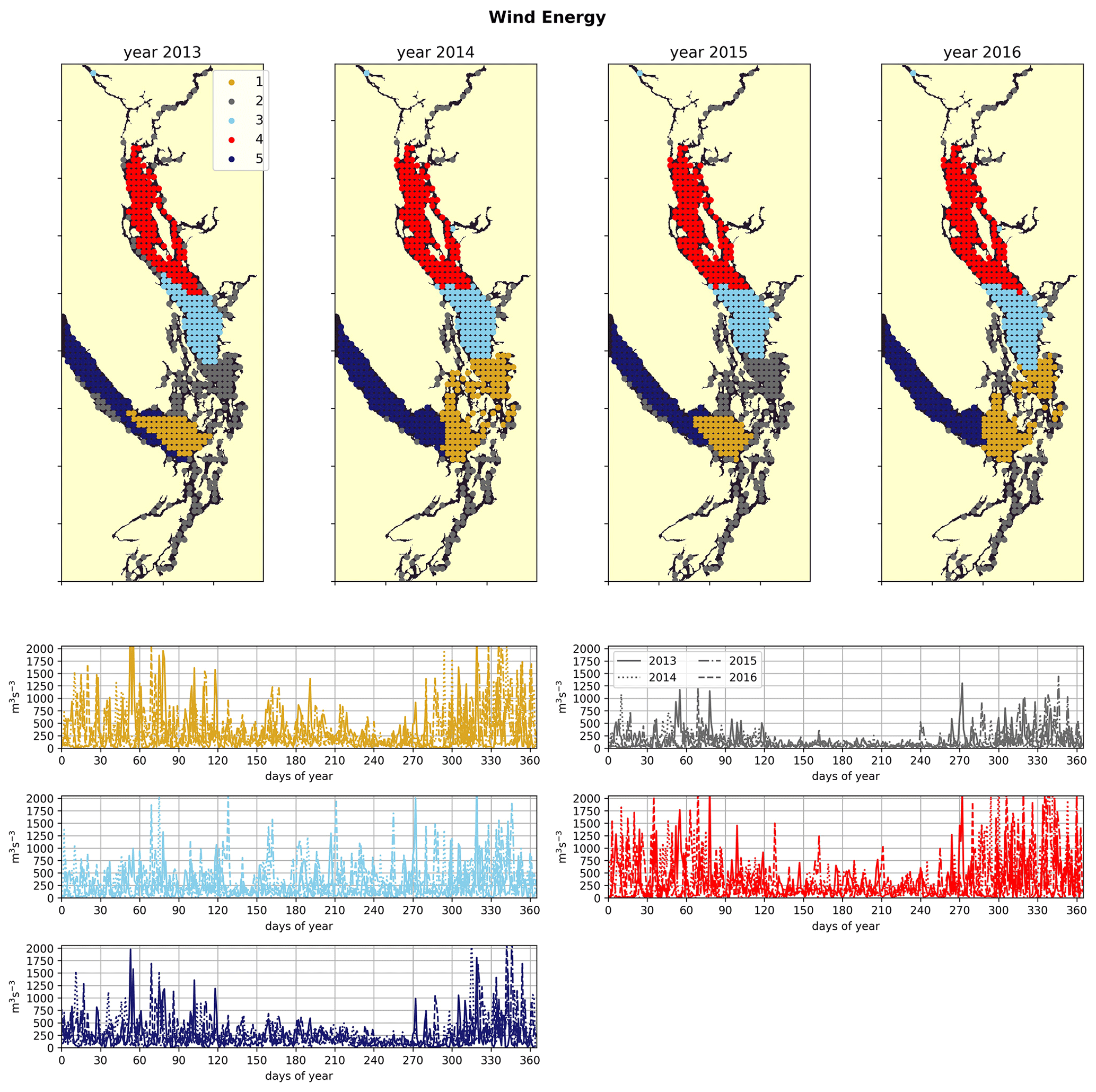
Figure 5Clustering of the daily average wind energy signal. Though spatial cluster boundaries are consistent, wind energy in all clusters is highly episodic, and all wind clusters show a marked decrease in wind energy during the summer months. Nearshore ares have lowest wind energy owing to low fetch. Summer wind energies are higher in the CSoG than in the NSoG.
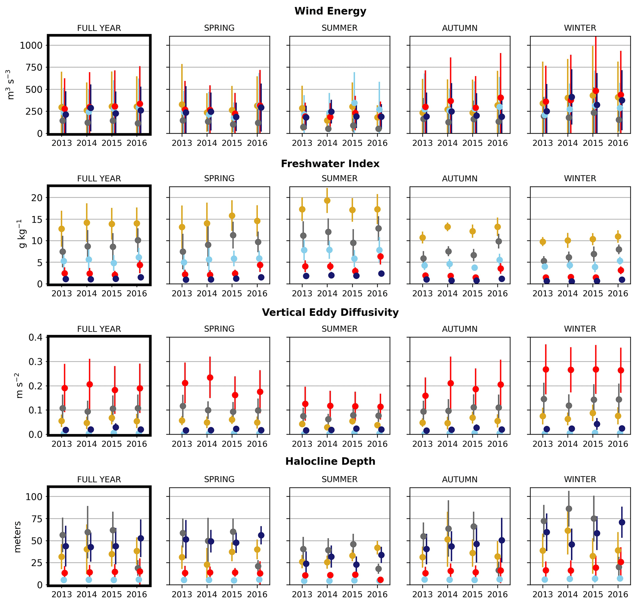
Figure 6Seasonal means of the physical signals. Seasons are defined as follows: winter is December–February, spring is March–May, summer is June–August, and fall is September–November. The temporal standard deviation of the seasonal mean signal for each cluster is shown.
In the wind clustering, the boundary between the CSoG and NSoG is farther south than that seen in the clusterings of freshwater index and halocline depth (Fig. 5). Though winds in all clusters are highly episodic, all wind clusters show a marked decrease in wind energy during the summer months (Fig. 6) – this change in mean signal magnitude and variability is most pronounced in the NSoG (cluster 4/red), which consistently shows ∼ 2 times higher wind energies in the winter months than in the summer months. In contrast, the CSoG (cluster 3/sky blue) shows the lowest variability between summer and winter energy magnitudes. Summer wind energies are actually higher in the CSoG than in the NSoG, likely due to the long wind fetch length in the CSoG, as summer winds in the Salish Sea are predominantly northerly (Thomson, 1981; Moore-Maley and Allen, 2022). Average vertical eddy diffusivity is lowest in the CSoG (Fig. 7), likely owing to both high stratification and comparatively low tidal currents (Thomson, 1981), consistent with the historical idea of the Salish Sea as a system of relatively quiet basins interconnected by dynamic sills (Ebbesmeyer and Barnes, 1980).
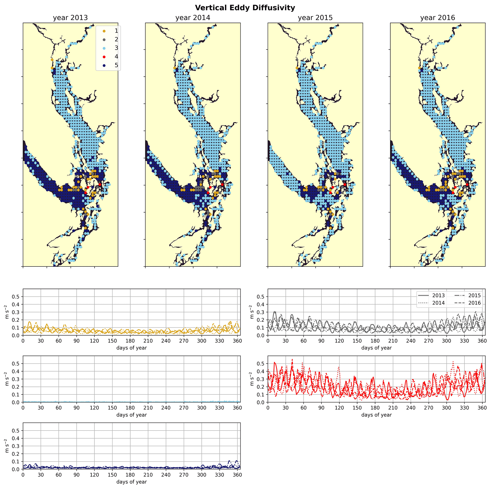
Figure 7Clustering of the daily depth-averaged vertical eddy diffusivity signal. The domain is split into two major regions: the Strait of Georgia, which has universally low vertical eddy diffusivity, and Juan de Fuca Strait, with comparatively slightly higher VED due to stronger tidal currents. VED hotspots of various magnitudes are consistently found at tidal mixing hotspots, including Discovery Passage near Seymour Narrows and Haro Strait near the San Juan islands.
3.2 Northern Strait of Georgia
As expected, the influence of the Fraser River is lower in the NSoG as the region is farther away from the river mouth (Fig. 3). The resulting lower stratification is reflected in deeper and more variable haloclines in all seasons (on average, ∼ 10 m in summer to ∼ 20 m in winter) (Fig. 4). A striking feature in the clustering of the freshwater index signal and halocline signals in the NSoG and the CSoG is the dissimilarity of the year 2016 to other years, reflected in a lower cluster persistence metric in this year (Fig. C2). Maximum Fraser River discharge (freshet) during 2016 was remarkably low, in the lowest quartile of discharge on record, reaching only ∼ 8000 m3 s−1, or roughly of the magnitude of the 2013–2014 freshets, which were both in the highest quartile (Fig. C3). Interestingly, the mean freshwater index signal for each cluster in 2016 remains similar to the means for other years, as does the spatial extent of the most river-influenced cluster (cluster 1/gold), but the medium freshwater-influenced clusters (cluster 2/grey, cluster 3/sky blue) extend less far from the river mouth. As a result, the NSoG clusters with JdF in this year.
3.3 Juan de Fuca Strait
Dynamics in Juan de Fuca Strait are broadly characterized by limited local freshwater influence, though a small increase in freshwater index is visible in the summer months (Figs. 3, 6), in part because of the surface advection of freshet-driven water from the CSoG due to the estuarine circulation (Thomson et al., 2007). The limited freshwater stratification, accompanied by a large tidal range, results in deep and variable haloclines (Fig. 4). The larger tidal velocities here are also reflected in slightly higher water-column-averaged VED (Fig. 7). Interestingly, in 2015, the VED in much of JdF clusters with the SoG, possibly due to the inhibition of water column mixing by higher thermal stratification of the system due to the significant marine heatwave in the North Pacific in the years 2013–2015 (Gentemann et al., 2017), whose effects were most pronounced in the Salish Sea in 2015 (Chandler et al., 2016). The dissimilarity of the year 2015 to other years is reflected in the cluster persistence metric (Fig. C2).
3.4 Tidal mixing hotspots
Water-column-averaged vertical eddy diffusivity in the Salish Sea is dominated by tidal mixing activity (Crean, 1978), allowing clustering VED to uncover dominant tidal hotspots. VED varies by 3 orders of magnitude in the model domain (Fig. 7). As expected, this metric reaches its maximum in the Haro Strait region, as well as in parts of Puget Sound, for example in Admiralty Inlet, near known tidal mixing hotspots (Ebbesmeyer and Barnes, 1980; LeBlond, 1983; Moore et al., 2008; Deppe et al., 2018). Two stations in northern Johnstone Strait and the Discovery Passage region also exhibit heightened VED in all 4 years, consistent with the high observed tidal velocities near Seymour Narrows in this region (Thomson, 1981). Fourier analysis of the annual vertical eddy diffusivity signals also shows local maxima in energy at weekly and fortnightly frequency (not shown) in all 4 years in all five clusters, consistent with the role of tides as the dominant source of mixing energy in the system (Crean, 1978).
The by-cluster seasonally averaged means and standard deviations of average VED are consistent interannually (Figs. 6, 7). The same three stations in the San Juan islands (cluster 4/red) report the highest VED in all 4 analyzed years, exhibiting maxima that are almost a factor of 2 larger than the next-largest signal (cluster 2/grey). In the highly variable Haro Strait and Johnstone Strait regions, the spatial frequency of our sampling likely plays a role in our derived map of tidal mixing hotspots – as we sample only approximately every 100th horizontal model coordinate, we likely miss other high-VED model points in this subregion, especially channels that have width scales comparable to our model resolution (0.5 km), for example the intricate channel passages of the San Juan and Discovery Island groups in the Haro and Johnstone Strait regions, which are known tidal mixing hotspots (Fig. 1). Analysis of tidal mixing hotspots is not the focus of this work, but a full characterization of this tidally mixed zone using a more refined clustering approach may be an interesting focus of future work.
3.5 Biomass of primary producers
A similar biological clustering arises in all 4 years (Figs. 8, C2). The boundaries of this clustering broadly coincide with the three major oceanographic subregions discussed above. The largest cluster (the CSoG – cluster 3/sky blue) is characterized by diatoms blooming first, followed by a transition to flagellate abundance in the summer months. In all 4 years, a functionally distinct NSoG region (cluster 4/red) arises, with sharp, episodic spikes in summer diatom biomass and diminished flagellate biomass. JdF (cluster 5/dark blue) reaches maximum biomass later in the year and, like the NSoG, shows a persistence of summer diatoms and diminished summer flagellate biomass. In contrast to the NSoG, where diatom biomass diminishes between episodic spikes, diatom biomass in JdF typically remains above 20 mmol N m−2 throughout the spring and summer seasons, with occasional spikes to higher biomass.
These three main regions have roughly similar mean seasonal biomass, with interannual variability larger than variability between clusters; the main differences between them are in the relative abundances of different functional groups and in the temporal characteristics of the phytoplankton biomass. Nearshore areas cluster together (cluster 2/grey) and have low depth-integrated biomass because they are limited by shallow depth. The largest depth-integrated biomass in the model in both the diatom and flagellate groups is found in the tidal mixing region of Haro Strait (cluster 1/gold).
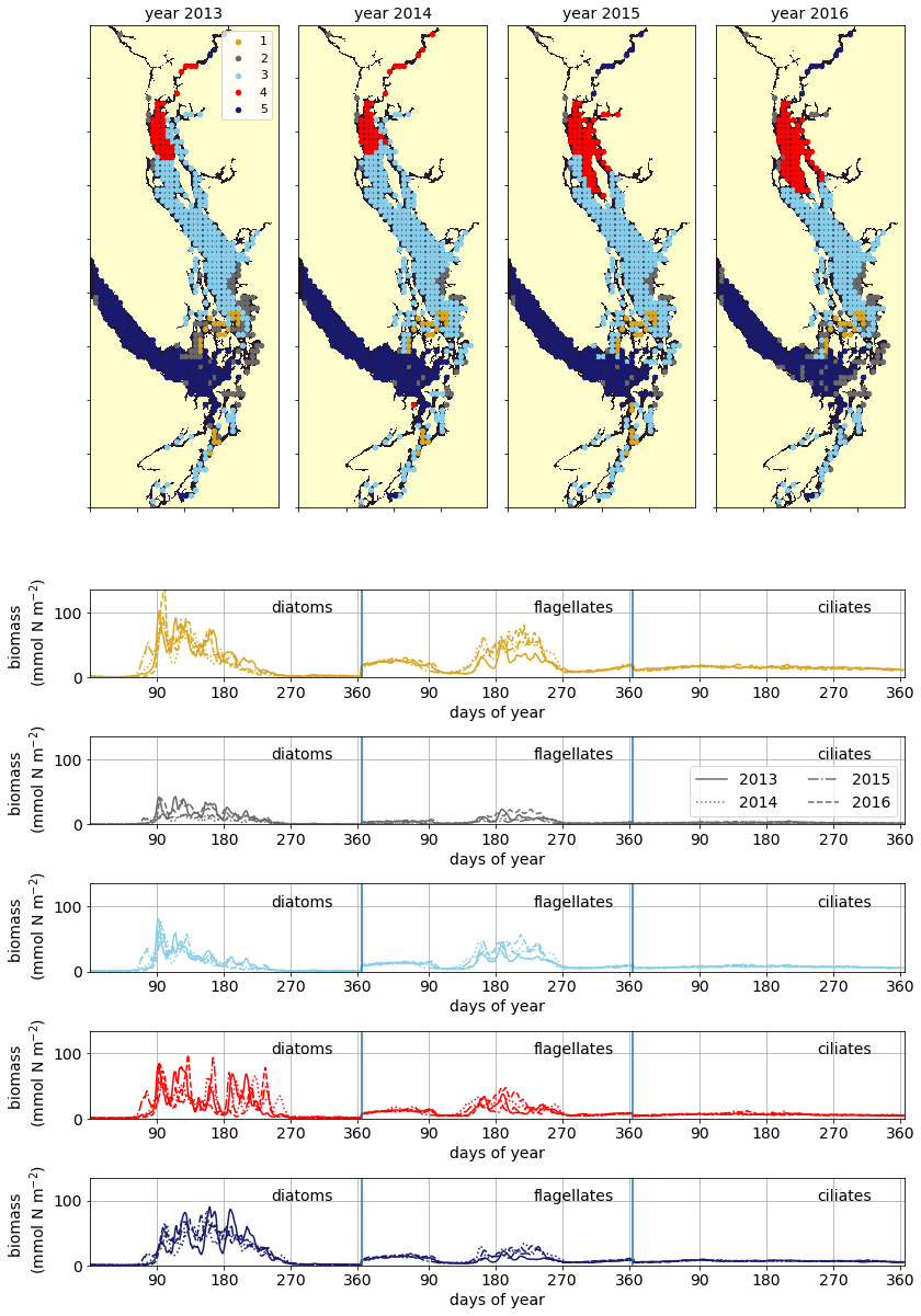
Figure 8Clustering of vertically integrated phytoplankton biomass separated by model-defined functional group (diatoms, followed by flagellates, then ciliates). The domain is split into the CSoG, NSoG, and JdF, each of which exhibits distinct phytoplankton dynamics (see Sect. 3.5 and the Discussion section).
We now consider the regional phytoplankton structure in the context of previous observational and modeling studies and discuss some mechanisms underlying the observed patterns. We focus on the three main regions found by the biological clustering (the CSoG, the NSoG, and JdF).
4.1 The northern vs. the central Strait of Georgia
In the model, the NSoG shows only slightly higher depth-averaged phytoplankton biomass in all seasons than the CSoG (Fig. 9). This biomass is consistent with the in situ study of Masson and Peña conducted between 2001 and 2007 in this region, which shows lower surface chlorophyll but a deeper phytoplankton growing zone in the NSoG, leading to slightly higher depth-integrated chlorophyll concentrations in the northern region in all four seasons of sampling (Masson and Peña, 2009, henceforth MP09, their Table 2). Remote sensing observations also show significantly lower surface chlorophyll in the NSoG throughout the year, as well as finding anomalously high surface chlorophyll concentrations in 2015 that are not reproduced by the model (Suchy et al., 2019). The majority of the modeled biomass difference between the NSoG and CSoG occurs in the subsurface maximum around 6–8 m in depth (Fig. C4), where it cannot be detected by remote sensing. Previous modeling (of the years 2007–2009) found somewhat higher depth-integrated phytoplankton biomass in the CSoG throughout the year, but with significant spatiotemporal variability (Peña et al., 2016). However, a recent year-round in situ campaign in several parts of the Strait of Georgia found no meaningful difference in depth-integrated chlorophyll between the NSoG and CSoG (Pawlowicz et al., 2020).
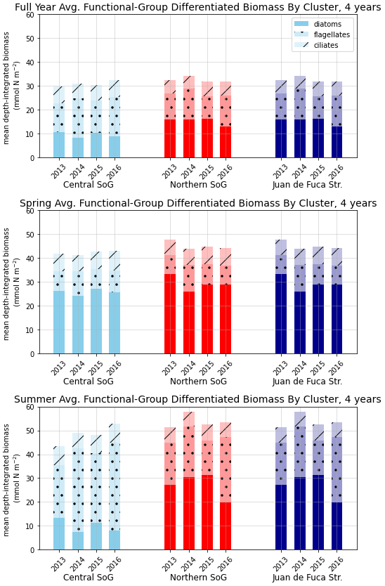
Figure 9Depth-integrated phytoplankton biomass for the three main biological clusters (CSoG, NSoG, and JdF) differentiated by functional group. The annual, spring, and summer means of the derived clusters are shown for all 4 modeled years. All three clustered regions have similar total biomass, which stays relatively consistent interannually, but functional group composition varies by cluster, with higher summer diatom abundance in the NSoG and JdF than in the CSoG. Spring is defined as March–May, and summer is June–August.
Together, these studies suggest that the difference between the two regions with respect to total depth-integrated biomass is subtle. However, we find a substantial difference in the modeled phytoplankton functional group composition and the temporal scale of variability of the phytoplankton signal between regions. In both regions of the strait, the opportunist-class diatoms, which have the highest growth rate and highest nutrient requirements, peak first (typically in late March, though with considerable variability; Allen and Wolfe, 2013) and form the majority of the phytoplankton biomass in the spring (Figs. 8, 9). In the CSoG, the model then transitions to higher biomass of gleaner-type flagellates around day 150, near the beginning of June, and flagellates continue to exhibit high summer biomass in this region (Figs. 8, 9). In contrast, the NSoG continues to exhibit episodic short-lived peaks of high opportunist-type phytoplankton biomass, represented by diatoms, throughout the summer so that in all years except 2016, diatoms make up the majority (∼ 55 %–60 %) of summer phytoplankton biomass in this region.
In the Strait of Georgia, significant evidence of high summer biomass near strong mixing zones or in response to mixing driven-nutrient delivery exists. For example, early surveys of the system find high chlorophyll associated with dynamic frontal regions in the northern and southern ends of the SoG (Parsons et al., 1981), and they consequently warn against drawing firm conclusions about the nature of phytoplankton abundance and variability from episodic sampling in shifting frontal zones. Nutrient delivery via episodic tidal mixing events near Discovery Passage has been linked to increased biomass (e.g., Parsons et al., 1981; Haigh and Taylor, 1991) and modeled primary productivity (Olson et al., 2020). Though this phenomenon has been recorded in the CSoG as well (Yin et al., 1997; St. John et al., 1993), higher stratification may dampen the magnitude of the nutrient pulses. Sudden introduction of abundant nutrients is expected to favor the opportunist functional group represented by diatoms over the slower-growing gleaner functional group represented by flagellates, as is seen in our clustering (Cloern and Dufford, 2005; Dutkiewicz et al., 2009). A recent 4-year time series of phytoplankton composition data at a station near Quadra Island in the NSoG supports this idea by showing episodic blooms of summer diatoms after wind events (Del Bel Belluz et al., 2021). Indirect evidence of episodic high biomass, sometimes following wind events, has been observed elsewhere in the NSoG (Evans et al., 2019; Mahara et al., 2021).
We suggest that our results reflect a controlling influence of stratification on phytoplankton biomass and community structure. Strong stratification concentrates phytoplankton biomass in a thin well-lit surface layer while limiting supply of nutrients after the initial biological drawdown. In the model, these conditions favor high abundance of the gleaner flagellate group. In the NSoG, nutrient drawdown also occurs, but episodic wind events lead to stronger upwelling and mixing due to the comparatively weaker stratification and inject sharp pulses of nutrients into the near surface, leading to sharp, short-lived diatom blooms (Moore-Maley and Allen, 2022). In contrast, in the CSoG, despite stronger summer winds, strong stratification continues to favor gleaner-type organisms. Faster-growing opportunist diatoms tend to outcompete gleaner flagellates when sufficient nutrients and light are available, but inherent variability in the physical environment promotes coexistence (Anderies and Beisner, 2000). The result is only a modest, if any, change in biomass but a significant change in functional group composition and temporal variability between the NSoG and CSoG.
Peña et al. find higher biomass in the CSoG due to the deeper nutricline in the NSoG (Peña et al., 2016). We find instead that the increased mixing in the NSoG provides increased nutrients and that biomass in both regions is about the same. These two views are not directly reconcilable and which view is more representative of actual conditions depends on accurately capturing the balance between the action of mixing as a source of nutrients and mixing as a source of light reduction and phytoplankton dilution.
4.2 Comparison with in situ phytoplankton functional group observations
The extent of phytoplankton diversity in the Salish Sea cannot be strictly condensed into the three functional groups represented in this model. The divide of the phytoplankton functional groups in the model does not precisely correspond to a split between diatoms and all types of flagellates. For instance, silicoflagellates (class Dictyochophyceae) might align with the diatom class based on silicon utilization. For this reason, we discuss these classes in terms of competition between opportunist-type primary producers with high nutrient needs and high light needs and gleaner-type primary producers with capacity to persist at lower nutrient and light levels. For this study, the requirement is capturing the overall regional biomass patterns and function. Here we provide a brief comparison between our results and available in situ phytoplankton functional group observations.
In situ measurements of the relative abundance of phytoplankton functional groups remain rare in the Salish Sea and tend to be sparse in space and/or time. In situ observations represent a snapshot at a single station and depth, while model output instead presents the average of a much larger volume (the discrete model cell). A recent temporally well-resolved 4-year (2015–2018) time series of phytoplankton biomass and composition, derived from high-performance liquid chromatography (HPLC) analysis of phytoplankton pigments, taken at a single station in the NSoG (Del Bel Belluz et al., 2021) provides a starting point for such a comparison. The in situ data, taken from a depth of 5 m, show diatom-dominated blooms with varying start dates in the spring season, followed by a transition to a regime wherein flagellate-type groups (chiefly prasinophytes and cryptophytes) make up the majority of phytoplankton biomass, but diatoms remain present (Del Bel Belluz et al., 2021, their Figs. 4, 5). Episodic later-summer diatom blooms occur in 3 of the 4 observational years, corroborating the modeled later-summer NSoG diatom blooms seen in this study.
Local phytoplankton composition data derived from shipboard observations from spring, summer, and autumn cruises spanning the Juan de Fuca Strait and both the CSoG and the NSoG are also available as a technical report by Nemcek et al. (2020). Unlike the Del Bel Belluz study, these data are relatively well-resolved in space but less resolved temporally; in a given year, typically only 1 d of observations is available for each station. The relative abundance of phytoplankton functional groups in the three regions is thus interannually variable (Nemcek et al., 2020, their Fig. 39-2), and in contrast to the Del Bel Belluz study, the data show only limited summer presence of diatoms in the NSoG in either of the years overlapping with our study (2015 and 2016). These observations contradict trends seen in our model. Simultaneously, these data show summer diatom dominance in the well-mixed Haro Strait region, corresponding to our tidal mixing region, which echoes trends we see in this study. Taken together, these two in situ phytoplankton composition studies each provide some corroboration of patterns we see in the model but differ from each other regarding summertime diatom representation in the NSoG. Combined with the modeling, these three perspectives on phytoplankton composition and biogeography each represent different spatial and temporal scales. The questions raised by their contrasting findings highlight the need for both modeling and observational work to provide a holistic view of the local biophysical dynamics.
Our modeling study is necessarily subject to limitations. For example, very high biomass shown in the tidal mixing region (Fig. 8, cluster 1/gold) could be an artifact of slower phytoplankton mortality rates, at least at times, than occur in nature, with phytoplankton mixed deep into the water column and persisting too long. Such a rate imbalance would affect the response to mixing described above. Available observations support model phytoplankton levels in this region but are limited to the upper water column. Because model–data agreement on biomass and nitrate is strong in these regions, we believe the mechanism of nutrient delivery by wind events in the less stratified north, leading to dominance of faster-growing phytoplankton, is robust.
4.3 Juan de Fuca Strait
Our results suggest that the mean annual average depth-integrated biomass is about the same in all three physical regions, including the well-mixed, weakly stratified JdF. In contrast, previous studies suggested a lower biomass in JdF (Masson and Peña, 2009; Peña et al., 2016) due to a deeper nutricline. However, recent in situ chlorophyll and nutrient data (2013–2016) support our result. In fact, the evaluation suggests that, for dates and locations for which observations are available, the model slightly underestimates observed biomass in Juan de Fuca Strait (Fig. A2, Table A2).
One factor contributing to the difference between these conclusions may be the vertical structure in the biomass observed by both MP09 and the model. In MP09, the spring phytoplankton biomass is much more prominent in the CSoG and NSoG than in JdF. The spring biomass exhibits a strong subsurface maximum (∼ 10 m in the chlorophyll observations) and persists relatively deep into the water column (up to 40 m). However, though overall concentrations reported in MP09 are lower in all seasons in JdF, observed chlorophyll concentrations >= 1 mg m−3 persist at deeper depths in most seasons in Juan de Fuca than in both regions of the Strait of Georgia (up to 50 m in the spring, summer, and fall), and in summer and fall, the NSoG exhibits slightly deeper phytoplankton persistence compared to the CSoG. We replicate these trends in general vertical structure (Fig. C4), with a prominent subsurface maximum at ∼ 6–8 m and phytoplankton biomass mixed deeper in Juan de Fuca Strait than in either region of the Strait of Georgia.
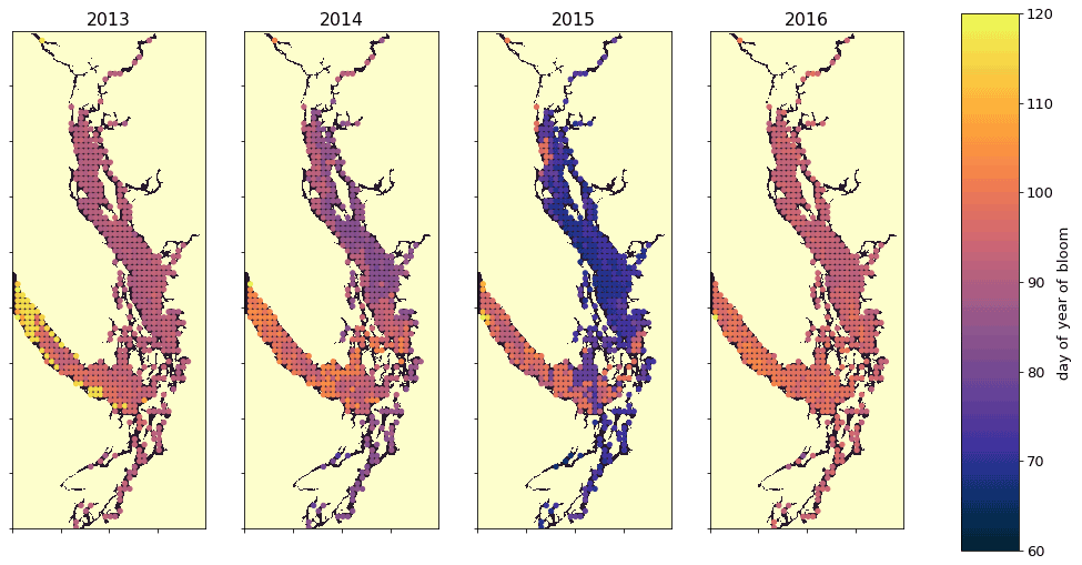
Figure 10A spatial view of the onset of the spring bloom in the domain. Here the spring bloom is defined as the first peak in depth-integrated diatom biomass that is at least 30 % of the maximum annual diatom biomass at that station. In all years, the spring bloom occurred earliest in the CSog and subsequently in the NSoG before reaching JdF with a variable delay.
This vertical structure likely leads to a dilution effect – even when phytoplankton concentration at a given depth may be lower in Juan de Fuca Strait than in the Strait of Georgia, overall depth-integrated biomass may be simultaneously higher. This deep biomass is less likely to be captured by sampling campaigns, potentially leading to an underestimation of the phytoplankton biomass of the region as a whole. Furthermore, because of the interannual variability in spring bloom timing and differences in spring bloom timing between the Strait of Georgia and Juan de Fuca Strait (discussed further below), the spring in situ survey that captures high biomass in the Strait of Georgia may be too early to observe the full extent of the spring bloom in Juan de Fuca Strait.
In the NSoG and CSoG, the derived biological signals suggest a regime wherein stable growing conditions in the spring transition to varying degrees of summer nutrient limitation which are interrupted by episodic nutrient delivery more frequently in the NSoG. In contrast, the diatom growth curve in JdF suggests a light-limited environment year-round, consistent with the established understanding (Mackas and Harrison, 1997). Nutrients are rarely limiting in JdF owing to the plentiful supply of oceanic nitrate (Sutton et al., 2013) and stronger water column mixing in this region demonstrated in the VED clustering (Fig. 7). One factor that may potentially enhance growing conditions in the summer season here is the advection of a freshwater lens from the Strait of Georgia via the surface estuarine circulation (Pawlowicz et al., 2007; MacCready et al., 2021). This advection is visible as a slight increase in the summer freshwater index in JdF (Fig. 6); it may contribute to increased water column stability and hence light availability and favorable growing conditions in this period.
4.3.1 Spring bloom timing
The timing of the first substantial increase in phytoplankton biomass (the spring bloom) in the Salish Sea varies considerably interannually and is driven by different factors, primarily wind speed and cloud cover and secondarily temperature and freshwater discharge (Allen and Wolfe, 2013). While we do not evaluate spring bloom timing here, considering the spatial variability of the onset of the spring bloom throughout the domain may deliver insights regarding the functioning of the different regions. For the purposes of this informal exploration, at each station we define the spring bloom as the first peak in depth-integrated diatom biomass that is at least 30 % of the maximum annual diatom biomass at that station. Earlier spring bloom initiation in the CSoG with respect to the NSoG was seen in multiple years of satellite observations (Suchy et al., 2019). In our results this progression within the SoG is almost indistinguishable and is followed by later blooming in the JdF. The late bloom timing in JdF was likely driven by stronger mixing, limiting light availability later into the year in the JdF region (Fig. 10), consistent with the functional differences between JdF and the NSoG and CSoG discussed above.
This preliminary examination of modeled bloom timing shows the large interannual variability in the onset of the spring bloom, consistent with one-dimensional models of the region (Collins et al., 2009; Allen and Wolfe, 2013) and the in situ and satellite-based observations (Suchy et al., 2019; Gower et al., 2013; Boldt et al., 2019). The significant spatial variability seen here underscores the dynamical differences in environmental growing conditions in different regions of the Salish Sea and provides an interesting direction for future research.
4.4 Utility of clustering methods in the context of high-resolution models
Our clustering approach identifies unambiguous regions of a complex coastal sea that exhibit distinct biological responses to disparate physical environments. These responses are not immediately obvious in time-averaged snapshots of the studied system. The simple machine learning technique used here enhances our way of looking at the problem – in this application, we are not using machine learning to predict unknown quantities, as is becoming common (e.g., Keppler et al., 2020), but instead we are asking it to show us what is already there. Using this simple technique, we are able to draw objective boundaries between regions based on emergent structures in our data and significantly advance our intuition about the system. Cluster-based model evaluation may also be a very useful application of clustering techniques, as it has potential to diagnose how well a given model performs across different biophysical regimes.
The simplicity of the approach may have utility in numerous contexts. For instance, many characterizations of environmental regions rely on sparse data with large spatial biases. Objective clusters determined from regional models, with mechanistic underpinnings, may be used to group sparse data. This approach allows clear characterization of complex systems. Furthermore, it may provide the necessary first step for machine learning studies that rely on well-organized training datasets to accurately predict target variables (e.g., Landschützer et al., 2013). Resource and environmental management situations and optimal monitoring strategies may also benefit from a data-driven approach to regional definitions.
Our work applies a hierarchical clustering algorithm to 4 years of SalishSeaCast model output. We extract four factors relating to stratification and one relating to depth-integrated phytoplankton biomass, differentiated by functional group. We identify distinct regions of the model domain that exhibit contrasting wind and freshwater input dynamics, as well as regions of varying water-column-averaged vertical eddy diffusivity and halocline depth regimes. Similar spatial regionalizations in physical variables persist in all 4 analyzed years.
Similarly, we find distinct, interannually persisting, biological regions with phytoplankton biomass patterns that may be explained by patterns in the physical factors. In the NSoG, a deeper winter halocline and episodic summer mixing coincide with higher summer opportunist-type phytoplankton abundance, represented in the model by diatoms, and episodic fluctuations in phytoplankton biomass. In contrast, in the Fraser River stratified CSoG, shallower haloclines and stronger summer stratification coincide with more consistent biomass and high summer abundance of gleaner-type phytoplankton with slower growth rates, represented in the model as the flagellate functional group. While the biomass signals in the CSoG and NSoG suggest varying degrees of nutrient limitation, the JdF biomass signal suggests a light-limited physical regime. Furthermore, the cluster-based model evaluation suggests that JdF supports more biomass here than previously thought, likely due to a deeper growing layer. Our approach shows that stratification controls nutrient delivery and causes subtle structure in regional biological patterns, and it demonstrates the utility of simple machine learning tools in extracting insight from large datasets in the context of oceanographic models.
We evaluate the version of the SalishSeaCast biophysical model used in this clustering analysis regionally against available data from the Department of Fisheries and Oceans Canada (Ocean Sciences Division, 2020), specifically nitrate, dissolved silica, log-transformed chlorophyll, absolute salinity, and conservative temperature, along with the spread of locations and times of collection (Figs. A1, A2; Tables A1, A2).
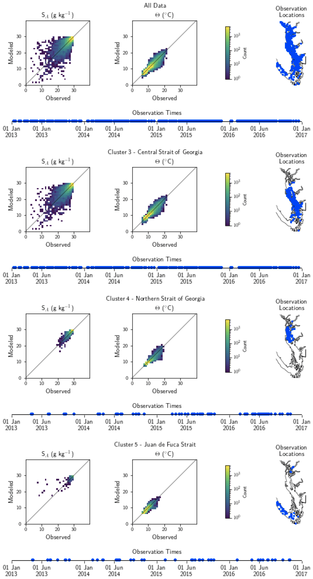
Figure A1Model comparison with DFO CTD (conductivity–temperature–depth sensor) temperature and salinity data. The plots show modeled vs. observed values for salinity and temperature for the entire model domain, as well as points matched only to the three major biological clusters – the northern Strait of Georgia, the central Strait of Georgia, and the Juan de Fuca Strait (cluster boundaries are specific to the year of observation) (note that in some years, Bute Inlet clusters with the Juan de Fuca Strait). Because of the large amount of data available for comparison, a histogram view is presented. The timeline and rightmost panel display observation times and locations. Summary statistics corresponding to these plots are shown in Table A1.
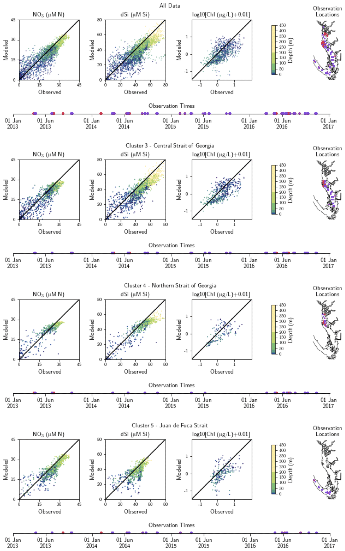
Figure A2Model comparison with DFO nitrate, dissolved silica, and log-transformed chlorophyll data. The plots show modeled vs. observed values for nitrate, dissolved silica, and log-transformed chlorophyll for the entire model domain, as well as points matched only to the three major biological clusters – the northern Strait of Georgia, the central Strait of Georgia, and the Juan de Fuca Strait (cluster boundaries are specific to the year of observation). The timeline and rightmost panel display observation times and locations. Stations with nutrients but no chlorophyll data are shown in red, while stations with observations of all three parameters are shown in purple. Summary statistics corresponding to these plots are shown in Table A2.
Table A1Summary statistics corresponding to the model–data comparison of temperature and salinity shown in Fig. A1. Model bias is low compared to model means, and model bias and skill score do not vary significantly between biological clusters.
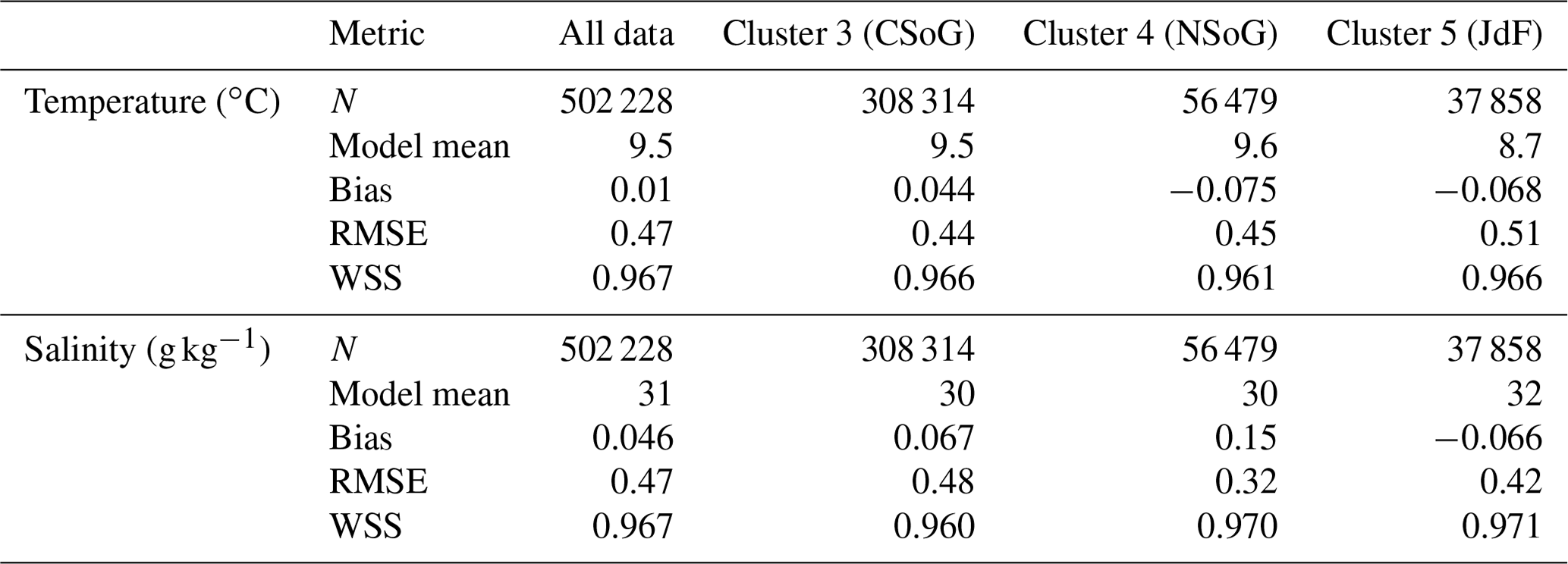
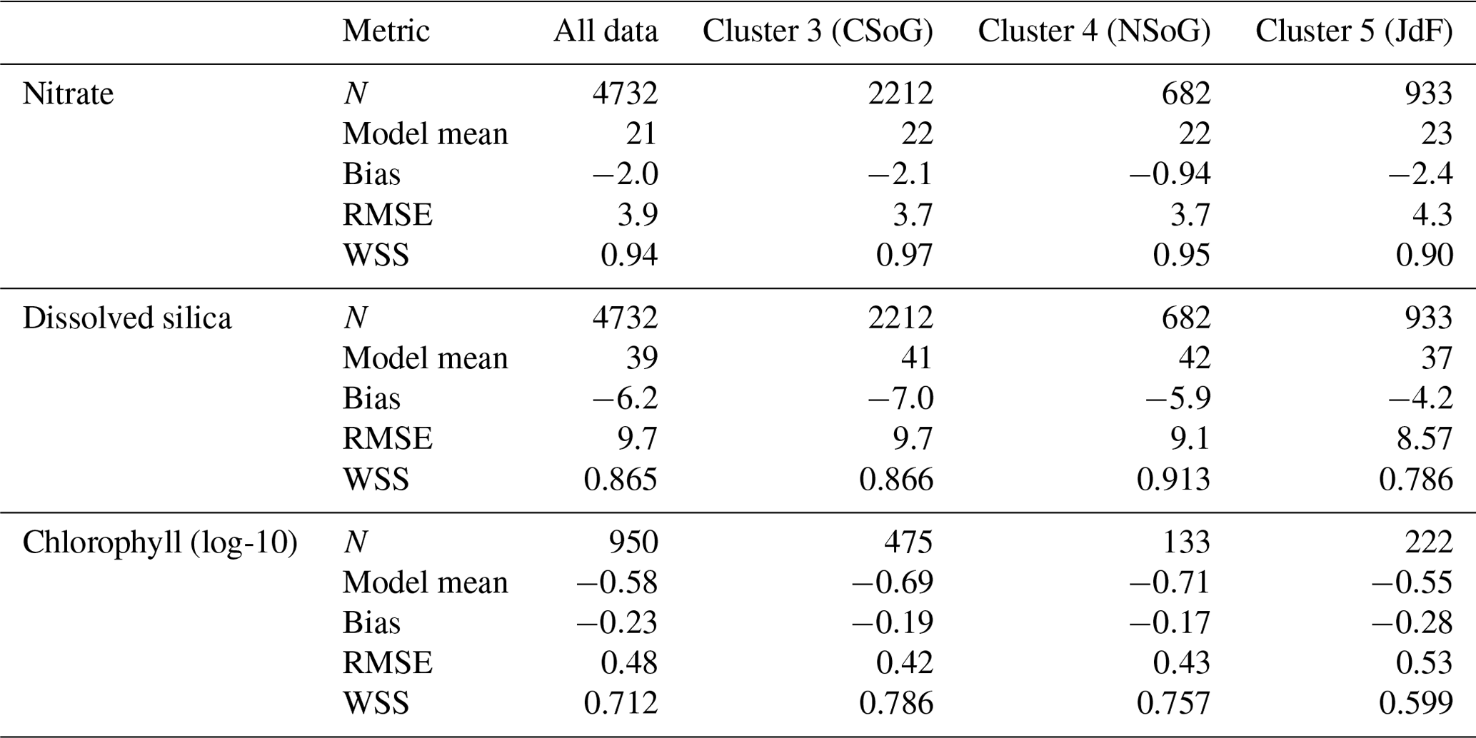
Table A2Summary statistics corresponding to the model–data comparison of biological variables shown in Fig. A2. Chlorophyll data are log-10 transformed. Model bias is low compared to model means and RMSE, and model bias and skill score do not vary significantly between biological clusters.
Several adjustments to the biological model have been made from the simulation described in Olson et al. (2020) for the present run. The most significant concerns the silicon cycle. The rate of silica dissolution was adjusted from to s−1, and a bottom flux of silicon of mmol m−2s−1 was added across the land–ocean interface below 250 m. The sinking rate of biogenic silicon was increased from to m s−1. The bottom reflection coefficient for biogenic silicon was increased from 0.8 to 0.92, and the reflection coefficient for diatoms was changed from 0.8 to 0. Additionally, the ratio of diatom silicon to nitrogen content was increased from 1.5 to 1.8 µmol Si : µmol N.
Diatom growth parameters were adjusted slightly, with an increase in the optimal light level from 42 to 45 W m−2, an increase in the dissolved silica half-saturation constant from 1.2 to 2.2 µM Si, and a 1 % decrease in maximum growth rate. The flagellate half-saturation constant for ammonium increased from 0.1 to 0.2 µM N.
Several small adjustments were made to grazing rates, prey preferences, and predation threshold, primarily to decrease the minimum standing stock of phytoplankton and increase grazing by microzooplankton relative to mesozooplankton. Additionally, the seasonally varying mesozooplankton maximum grazing level was adjusted slightly, decreasing winter and midsummer grazing rates and bringing the cycle forward by approximately 5 d. The western boundary and riverine nutrient concentrations have been updated. The namelists specifying these small adjustments are available from the paper's associated GitHub repository.

Figure C1One example clustering output by Ward's method for the annual halocline depth signal in the year 2015 (see Sect. 2.2–2.3).
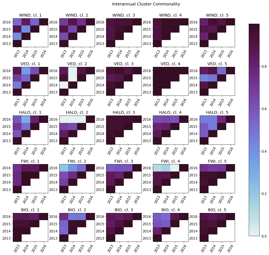
Figure C2The interannual cluster commonality metric, measuring interannual cluster persistence for each factor. For any two clusters, cluster commonality varies from 0 (clusters of any size with no stations in common) to 1 (two clusters of equal size with all stations in common) and may be used to compare clusters of unequal sizes.
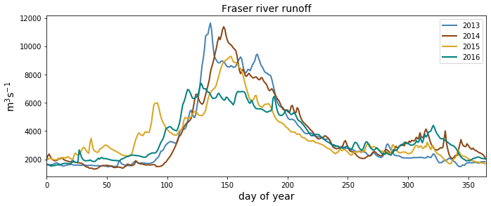
Figure C3Fraser river flow at Hope, British Columbia, for the 4 modeled years, as implemented in Soontiens and Allen (2017). Data from Environment and Climate Change Canada (https://wateroffice.ec.gc.ca/report/real_time_e.html?stn=08MF005, last access: June 2021).
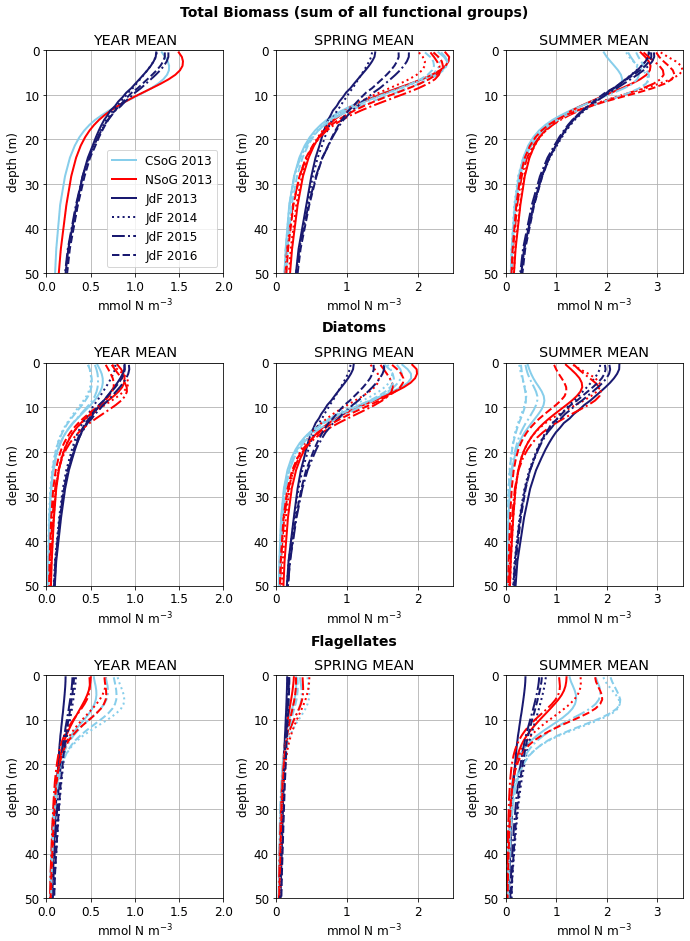
Figure C4Mean depth profiles of phytoplankton biomass for the three main biological clusters (CSoG, NSoG, and JdF) for all 4 modeled years. Spring is defined as March–May, summer is June–August, autumn is September–November, and winter is December–February.
Model namelists as well as post-processing and analysis scripts are available from the associated GitHub repository (https://doi.org/10.5281/zenodo.7144696, Jarníková, 2022a). SalishSeaCast results are available from the SalishSeaCast ERDDAP server (https://salishsea.eos.ubc.ca/erddap/index.html, SalishSeaCast Project Contributors, 2022). Observational data used in the model evaluation are available online from the Department of Fisheries and Oceans Canada (DFO): https://www.pac.dfo-mpo.gc.ca/science/oceans/data-donnees/index-eng.html (DFO, 2016). More information about SalishSeaCast can be found on the project web page (https://salishsea.eos.ubc.ca, last access: 10 May 2022). The model source code is available at https://doi.org/10.5281/zenodo.7144812, (Jarníková, 2022b).
TJ developed the cluster analysis with significant input from SEA and DI. EMO developed and tuned the biological model and developed the basis for the model evaluation. TJ wrote the paper with significant scientific input from EMO, SEA, DI, and KDS. TJ is supervised by SEA and DI.
The contact author has declared that neither they nor their co-authors have any competing interests.
Publisher's note: Copernicus Publications remains neutral with regard to jurisdictional claims in published maps and institutional affiliations.
The SalishSeaCast software environment was developed by Doug Latornell. Tereza Jarníková thanks Valentina Radic for the insightful data science course that inspired the concept of the study, as well as the Mesoscale Ocean and Atmospheric Dynamics group at the University of British Columbia for the collegial atmosphere and valuable feedback.
This work was funded by the Marine Environmental Observation, Prediction and Response (MEOPAR) Network of Canada (grant numbers 1.2, 7.2, and 65.9), as well as by the Natural Sciences and Engineering Research Council of Canada (NSERC) Discovery Grant (grant number RGPIN-2016-03865) and the Government of Canada's Aquatic Climate Change Adaptation and Services Program (ACCASP). Computational resources were provided by Compute Canada for hindcast runs (grant numbers FT520, RRG2648, and RRG2969). Tereza Jarníková was partially funded by a personal Four-Year Fellowship through the University of British Columbia.
This paper was edited by Bernadette Sloyan and reviewed by Jennifer Jackson and one anonymous referee.
Allen, S. and Wolfe, M.: Hindcast of the timing of the spring phytoplankton bloom in the Strait of Georgia, 1968–2010, Prog. Oceanogr., 115, 6–13, 2013. a, b, c
Anderies, J. M. and Beisner, B. E.: Fluctuating environments and phytoplankton community structure: a stochastic model, Am. Nat., 155, 556–569, 2000. a
Boldt, J. L., Thompson, M., Rooper, C. N., Hay, D. E., Schweigert, J. F., Quinn II, T. J., Cleary, J. S., and Neville, C. M.: Bottom-up and top-down control of small pelagic forage fish: factors affecting age-0 herring in the Strait of Georgia, British Columbia, Mar. Ecol.-Prog. Ser., 617, 53–66, 2019. a, b
Chandler, P. C., King, S. A., and Perry, R. I. (Eds.): State of the physical, biological and selected fishery resources of Pacific Canadian marine ecosystems in 2016, Department of Fisheries and Oceans, ISBN 978-0-660-09251-5, 2016. a
Cloern, J. E. and Dufford, R.: Phytoplankton community ecology: principles applied in San Francisco Bay, Mar. Ecol.-Prog. Ser., 285, 11–28, 2005. a
Collins, A. K., Allen, S. E., and Pawlowicz, R.: The role of wind in determining the timing of the spring bloom in the Strait of Georgia, Can. J. Fish. Aquat. Sci., 66, 1597–1616, 2009. a
Crean, P.: A Numerical Model of Barotropic Mixed Tides Between Vancouver Island and the Mainland and its Relation to Studies of the Estuarine Circulation, Elsev. Oceanogr. Serie., 23, 283–313, 1978. a, b, c
Del Bel Belluz, J., Peña, M. A., Jackson, J. M., and Nemcek, N.: Phytoplankton Composition and Environmental Drivers in the Northern Strait of Georgia (Salish Sea), British Columbia, Canada, Estuar. Coast., 44, 1419–1439, 2021. a, b, c
Deppe, R. W., Thomson, J., Polagye, B., and Krembs, C.: Predicting deep water intrusions to Puget Sound, WA (USA), and the seasonal modulation of dissolved oxygen, Estuar. Coast., 41, 114–127, 2018. a
DFO: Institute of Ocean Sciences Data Archive, Ocean Sciences Division, Department of Fisheries and Oceans Canada [data set], https://www.pac.dfo-mpo.gc.ca/science/oceans/data-donnees/index-eng.html (last acces: 10 February 2020), 2016. a
Dutkiewicz, S., Follows, M. J., and Bragg, J. G.: Modeling the coupling of ocean ecology and biogeochemistry, Global Biogeochem. Cy., 23, GB4017, https://doi.org/10.1029/2008GB003405, 2009. a
Ebbesmeyer, C. C. and Barnes, C. A.: Control of a fjord basin's dynamics by tidal mixing in embracing sill zones, Estuar. Coast. Mar. Sci., 11, 311–330, 1980. a, b
Evans, W., Pocock, K., Hare, A., Weekes, C., Hales, B., Jackson, J., Gurney-Smith, H., Mathis, J. T., Alin, S. R., and Feely, R. A.: Marine CO2 patterns in the northern Salish Sea, Frontiers in Marine Science, 5, 536, https://doi.org/10.3389/fmars.2018.00536, 2019. a
Field, C. B., Behrenfeld, M. J., Randerson, J. T., and Falkowski, P.: Primary production of the biosphere: integrating terrestrial and oceanic components, Science, 281, 237–240, 1998. a
Fischer, H., List, E., Koh, R., Imberger, J., and Brooks, N.: Mixing in inland and coastal waters, Academic Press, ISBN 978-0-08-051177-1, 1979. a
Follows, M. J., Dutkiewicz, S., Grant, S., and Chisholm, S. W.: Emergent biogeography of microbial communities in a model ocean, Science, 315, 1843–1846, 2007. a
Gentemann, C. L., Fewings, M. R., and García-Reyes, M.: Satellite sea surface temperatures along the West Coast of the United States during the 2014–2016 northeast Pacific marine heat wave, Geophys. Res. Lett., 44, 312–319, 2017. a
Giddings, S. N. and MacCready, P.: Reverse Estuarine Circulation Due to Local and Remote Wind Forcing, Enhanced by the Presence of Along-Coast Estuaries, J. Geophys. Res.-Oceans, 122, 10184–10205, https://doi.org/10.1002/2016JC012479, 2017. a
Gower, J., King, S., Statham, S., Fox, R., and Young, E.: The Malaspina Dragon: a newly-discovered pattern of the early spring bloom in the Strait of Georgia, British Columbia, Canada, Prog. Oceanogr., 115, 181–188, 2013. a
Grover, J. P.: Resource competition in a variable environment: phytoplankton growing according to Monod's model, Am. Nat., 136, 771–789, 1990. a
Grover, J. P., HUDZIAK, J., and Grover, J. D.: Resource competition, Vol. 19, Springer Science & Business Media, ISBN 978-1-4615-6397-6, 1997. a
Haigh, R. and Taylor, F.: Mosaicism of microplankton communities in the northern Strait of Georgia, British Columbia, Mar. Biol., 110, 301–314, 1991. a
Huisman, J., Sharples, J., Stroom, J. M., Visser, P. M., Kardinaal, W. E. A., Verspagen, J. M., and Sommeijer, B.: Changes in turbulent mixing shift competition for light between phytoplankton species, Ecology, 85, 2960–2970, 2004. a
Jarníková, T.: tjarnikova/CLUSTER_OS: Supplementary Code for Jarnikova et al. 2022 (v1.0.0), Zenodo [code], https://doi.org/10.5281/zenodo.7144696, 2022a. a
Jarníková, T.: SalishSeaCast/NEMO-3.6-CLUSTER: Model Source Code for Jarnikova et al. 2022 (v1.0.0), Zenodo [code], https://doi.org/10.5281/zenodo.7144812, 2022b. a
Keppler, L., Landschützer, P., Gruber, N., Lauvset, S., and Stemmler, I.: Seasonal Carbon Dynamics in the Near-Global Ocean, Global Biogeochem. Cy., 34, https://doi.org/10.1029/2020GB006571, e2020GB006571, 2020. a
Khangaonkar, T., Long, W., and Xu, W.: Assessment of circulation and inter-basin transport in the Salish Sea including Johnstone Strait and Discovery Islands pathways, Ocean Model., 109, 11–32, 2017. a
Landschützer, P., Gruber, N., Bakker, D. C. E., Schuster, U., Nakaoka, S., Payne, M. R., Sasse, T. P., and Zeng, J.: A neural network-based estimate of the seasonal to inter-annual variability of the Atlantic Ocean carbon sink, Biogeosciences, 10, 7793–7815, https://doi.org/10.5194/bg-10-7793-2013, 2013. a
LeBlond, P. H.: The Strait of Georgia: functional anatomy of a coastal sea, Can. J. Fish. Aquat. Sci., 40, 1033–1063, 1983. a, b, c
Legendre, L.: Hydrodynamic control of marine phytoplankton production: the paradox of stability, Elsev. Oceanogr. Serie., 32, 191–207, 1981. a
Liu, J.: Evaluation of a NEMO model of the Strait of Georgia and insights into mixing and transport of the Fraser River plume, Master's thesis, University of British Columbia, Vancouver, British Columbia, https://open.library.ubc.ca/cIRcle/collections/ubctheses/24/items/1.0343600 (last access: 20 April 2022), 2014. a
Longhurst, A., Sathyendranath, S., Platt, T., and Caverhill, C.: An estimate of global primary production in the ocean from satellite radiometer data, J. Plankton Res., 17, 1245–1271, 1995. a
MacCready, P., McCabe, R. M., Siedlecki, S. A., Lorenz, M., Giddings, S. N., Bos, J., Albertson, S., Banas, N., and Garnier, S.: Estuarine circulation, mixing, and residence times in the Salish Sea, J. Geophys. Res.-Oceans, 126, e2020JC016738, https://doi.org/10.1029/2020JC016738, 2021. a
Mackas, D. L. and Harrison, P. J.: Nitrogenous nutrient sources and sinks in the Juan de Fuca Strait/Strait of Georgia/Puget Sound estuarine system: assessing the potential for eutrophication, Estuar. Coast. Shelf S., 44, 1–21, https://doi.org/10.1006/ecss.1996.0110, 1997. a
Madec, G., Bourdallé-Badie, R., Bouttier, P.-A., et al.: NEMO ocean engine. In Notes du Pôle de modélisation de l'Institut Pierre-Simon Laplace (IPSL) (v3.6-patch, Number 27), Zenodo [software documentation], https://doi.org/10.5281/zenodo.3248739, 2017. a
Mahara, N., Pakhomov, E., Dosser, H., and Hunt, B.: How zooplankton communities are shaped in a complex and dynamic coastal system with strong tidal influence, Estuar. Coast. Shelf S., 249, 107103, https://doi.org/10.1016/j.ecss.2020.107103, 2021. a
Malick, M. J., Cox, S. P., Mueter, F. J., and Peterman, R. M.: Linking phytoplankton phenology to salmon productivity along a north–south gradient in the Northeast Pacific Ocean, Can. J. Fish. Aquat. Sci., 72, 697–708, 2015. a
Mangiameli, P., Chen, S. K., and West, D.: A comparison of SOM neural network and hierarchical clustering methods, Eur. J. Oper. Res., 93, 402–417, 1996. a
Masson, D.: Deep water renewal in the Strait of Georgia, Estuar. Coast. Shelf S., 54, 115–126, 2002. a
Masson, D. and Peña, A.: Chlorophyll distribution in a temperate estuary: The Strait of Georgia and Juan de Fuca Strait, Estuar. Coast. Shelf S., 82, 19–28, 2009. a, b, c, d
Maulik, U. and Bandyopadhyay, S.: Performance evaluation of some clustering algorithms and validity indices, IEEE T. Pattern Anal., 24, 1650–1654, 2002. a
Milbrandt, J. A., Bélair, S., Faucher, M., Vallée, M., Carrera, M. L., and Glazer, A.: The pan-Canadian high resolution (2.5 km) deterministic prediction system, Weather Forecast., 31, 1791–1816, https://doi.org/10.1175/WAF-D-16-0035.1, 2016. a
Moore, S. K., Mantua, N. J., Newton, J. A., Kawase, M., Warner, M. J., and Kellogg, J. P.: A descriptive analysis of temporal and spatial patterns of variability in Puget Sound oceanographic properties, Estuar. Coast. Shelf S., 80, 545–554, 2008. a
Moore-Maley, B. and Allen, S. E.: Wind-driven upwelling and surface nutrient delivery in a semi-enclosed coastal sea, Ocean Sci., 18, 143–167, https://doi.org/10.5194/os-18-143-2022, 2022. a, b, c, d
Morrison, J., Foreman, M., and Masson, D.: A method for estimating monthly freshwater discharge affecting British Columbia coastal waters, Atmosphere-Ocean, 50, 1–8, 2012. a
Nemcek, N., Hennekes, M., and Perry, I.: Seasonal dynamics of the phytoplankton community in the Salish Sea from HPLC, in: State of the Physical, Biological and Selected Fishery Resources of Pacific Canadian Marine Ecosystems in 2019, edited by: Boldt, J. L., Javorski, A., and Chandler, P. C., chap. 39, 169–173, Canadian Technical Report of Fisheries and Aquatic Sciences 3377, ISBN 978-0-660-34961-9, 2020. a, b
Ocean Sciences Division (Department of Fisheries and Oceans Canada): Institute of Ocean Sciences Data Archive, http://www.pac.dfo-mpo.gc.ca/science/oceans/data-donnees/index-eng.html (last access: 10 April 2022), 2020. a
Olson, E. M., Allen, S. E., Do, V., Dunphy, M., and Ianson, D.: Assessment of Nutrient Supply by a Tidal Jet in the Northern Strait of Georgia Based on a Biogeochemical Model, J. Geophys. Res.-Oceans, 125, e2019JC015766, https://doi.org/10.1029/2019JC015766, 2020. a, b, c, d, e, f
Parsons, T., Stronach, J., Borstad, G., Louttit, G., and Perry, R.: Biological fronts in the Strait of Georgia, British Columbia, and their relation to recent measurements of primary productivity, Mar. Ecol.-Prog. Ser., 6, 237–242, 1981. a, b
Pawlowicz, R., Riche, O., and Halverson, M.: The circulation and residence time of the Strait of Georgia using a simple mixing-box approach, Atmosphere-Ocean, 45, 173–193, 2007. a
Pawlowicz, R., Suzuki, T., Chappell, R., Ta, A., and Esenkulova, S.: Atlas of oceanographic conditions in the Strait of Georgia (2015–2019) based on the Pacific Salmon Foundation's Citizen Science Dataset, Canadian Technical Report of Fisheries and Aquatic Sciences, 3374, ISBN 9780660349367, 2020. a, b
Peña, M. A., Masson, D., and Callendar, W.: Annual plankton dynamics in a coupled physical–biological model of the Strait of Georgia, British Columbia, Prog. Oceanogr., 146, 58–74, 2016. a, b, c, d
Pike, R. G., Redding, T., Moore, R., Winkler, R., and Bladon, K. (Eds.): Compendium of forest hydrology and geomorphology in British Columbia, Land Management Handbook-Ministry of Forests and Range, in: For. Sci. Prog., Victoria, BC and FORREX Forum for Research and Extension in Natural Resources, Kamloops, BC Land Manag. Handb, Vol. 66, ISBN 978-0-7726-6332-0, 2010. a
Preikshot, D., Beamish, R. J., and Neville, C. M.: A dynamic model describing ecosystem-level changes in the Strait of Georgia from 1960 to 2010, Prog. Oceanogr., 115, 28–40, 2013. a
Richardson, A. J.: In hot water: zooplankton and climate change, ICES J. Mar. Sci., 65, 279–295, 2008. a
SalishSeaCast Project Contributors: griddap, SalishSeaCast ERDDAP server [data set], https://salishsea.eos.ubc.ca/erddap/index.html, last access: 4 October 2022. a
Sonnewald, M., Dutkiewicz, S., Hill, C., and Forget, G.: Elucidating ecological complexity: Unsupervised learning determines global marine eco-provinces, Sci. Adv., 6, eaay4740, https://doi.org/10.1126/sciadv.aay4740, 2020. a
Soontiens, N. and Allen, S. E.: Modelling sensitivities to mixing and advection in a sill-basin estuarine system, Ocean Model., 112, 17–32, 2017. a, b, c
Soontiens, N., Allen, S. E., Latornell, D., Le Souëf, K., Machuca, I., Paquin, J.-P., Lu, Y., Thompson, K., and Korabel, V.: Storm surges in the Strait of Georgia simulated with a regional model, Atmosphere-Ocean, 54, 1–21, 2016. a
St. John, M., Marinone, S., Stronach, J., Harrison, P., Fyfe, J., and Beamish, R.: A horizontally resolving physical–biological model of nitrate concentration and primary productivity in the Strait of Georgia, Can. J. Fish. Aquat. Sci., 50, 1456–1466, 1993. a
Suchy, K. D., Le Baron, N., Hilborn, A., Perry, R. I., and Costa, M.: Influence of environmental drivers on spatio-temporal dynamics of satellite-derived chlorophyll a in the Strait of Georgia, Prog. Oceanogr., 176, 102134, https://doi.org/10.1016/j.pocean.2019.102134, 2019. a, b, c, d, e
Sun, Q., Little, C. M., Barthel, A. M., and Padman, L.: A clustering-based approach to ocean model–data comparison around Antarctica, Ocean Sci., 17, 131–145, https://doi.org/10.5194/os-17-131-2021, 2021. a
Sutton, J. N., Johannessen, S. C., and Macdonald, R. W.: A nitrogen budget for the Strait of Georgia, British Columbia, with emphasis on particulate nitrogen and dissolved inorganic nitrogen, Biogeosciences, 10, 7179–7194, https://doi.org/10.5194/bg-10-7179-2013, 2013. a
Sverdrup, H.: On conditions for the vernal blooming of phytoplankton, J. Cons. Int. Explor. Mer., 18, 287–295, 1953. a
Thomson, R. E.: Oceanography of the British Columbia Coast, Canadian Special Publication of Fisheries and Aquatic Science, Fisheries and Oceans Canada, 291, ISBN 0-660-10978-6, 1981. a, b, c, d
Thomson, R., Mihály, S., and Kulikov, E.: Estuarine versus transient flow regimes in Juan de Fuca Strait, J. Geophys. Res., 112, C09022, https://doi.org/10.1029/2006JC003925, 2007. a
Umlauf, L. and Burchard, H.: A generic length-scale equation for geophysical turbulence models, J. Marine Res., 61, 235–265, 2003. a
Ward Jr., J. H.: Hierarchical grouping to optimize an objective function, J. Am. Stat. Assoc., 58, 236–244, 1963. a
Wasser, S. K., Lundin, J. I., Ayres, K., Seely, E., Giles, D., Balcomb, K., Hempelmann, J., Parsons, K., and Booth, R.: Population growth is limited by nutritional impacts on pregnancy success in endangered Southern Resident killer whales (Orcinus orca), PLoS One, 12, e0179824, https://doi.org/10.1371/journal.pone.0179824, 2017. a
Wishart, D.: 256. Note: An algorithm for hierarchical classifications, Biometrics, 25, 165–170, 1969. a
Yin, K., Goldblatt, R. H., Harrison, P. J., John, M. A. S., Clifford, P. J., and Beamish, R. J.: Importance of wind and river discharge in influencing nutrient dynamics and phytoplankton production in summer in the central Strait of Georgia, Mar. Ecol.-Prog. Ser., 161, 173–183, 1997. a
- Abstract
- Introduction
- Methods
- Results
- Discussion
- Conclusion
- Appendix A: Model evaluation
- Appendix B: Changes to biophysical model since first publication
- Appendix C: Companion figures
- Code and data availability
- Author contributions
- Competing interests
- Disclaimer
- Acknowledgements
- Financial support
- Review statement
- References