Technical note: On seasonal variability of the M₂ tide

Seasonal variability of the M₂ ocean tide can be detected at many ports, perhaps most. Examination of the cluster of tidal constituents residing within the M₂ tidal group can shed light on the physical mechanisms underlying seasonality. In the broadest terms these are astronomical, frictional–advective interactions, and climate processes; some induce annual modulations and some semiannual, in amplitude, phase, or both. This note reviews how this occurs and gives an example from each broad category. Phase conventions and their relationship with causal mechanisms, as well as nomenclature, are also addressed.

1 Introduction

It has long been noticed (Darwin, 1907; Corkan, 1934) that ocean tide constituents at some ports may experience significant seasonal variations. Especially noteworthy are large modulations discovered in some polar regions (e.g., Godin, 1986; Rotermund et al., 2021; Bij de Vaate et al., 2021). Significant modulations can also occur at lower latitudes, both regionally (Kang et al., 2002) and especially locally (e.g., Foreman et al., 1995). In fact, nearly all coastal tides show at least a small seasonal modulation (Pugh and Woodworth, 2014).

Climate-driven processes capable of inducing seasonal changes in barotropic tides are myriad: variability in ocean stratification (Müller, 2012), variability in ice cover (Prinsenberg, 1988), seasonal runoff and changes in river discharge (Guo et al., 2015), and tide–surge interactions from predominantly wintertime storms (Pugh and Woodworth, 2014). Similar processes and others can induce seasonal perturbations in baroclinic tides detectable in surface measurements (Ray and Zaron, 2011; Zhao, 2021). The extent the astronomical tidal potential plays in seasonality – usually small, but potentially important where tide amplitudes are large – is often overlooked. Some confusion on the issue was recently clarified by Du and Yu (2021).

To help unravel observations, it is useful to revisit the spectral characteristics behind seasonal variability. Understanding how certain spectral lines in observed sea level arise often points to possible physical mechanisms at work. The purpose of this note is to review this topic, focusing solely on the principal semidiurnal tide M₂. Much of what follows is hardly new; the purpose is to review and clarify, including even the nomenclature used. Whether seasonal variability is annual or semiannual, and whether it occurs in amplitude or phase or both, are obviously important aspects of variability; seeing one type of modulation rather than another can narrow the list of causes.

2 The M₂ tidal group

Recall the technical definitions (e.g., Munk and Cartwright, 1966) of “tidal group” – a cluster of spectral lines with the same first two Doodson numbers – and “tidal constituent” – a cluster with the same first three Doodson numbers. Tidal groups are separated in frequency by about one cycle per month, constituents by about one cycle per year. So when one speaks of seasonal variability of the M₂ tide, one must be speaking, in a sense, of the M₂ tidal group. It is the variability seen, for example, in a series of monthly estimates of M₂.

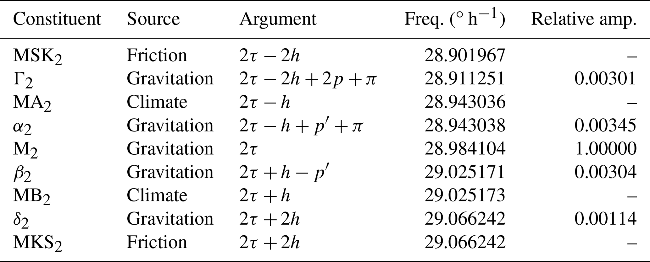
The main constituents within the M₂ group are listed in Table 1 in order of frequency. Included are tides generated by the astronomical potential (Cartwright and Edden, 1973; Hartmann and Wenzel, 1995), compound tides generated by shallow-water processes, and two annual sidelines (MA₂ and MB₂) commonly employed to effect an annual modulation from the wide range of possible climate processes. Climate processes are broadband, but they do commonly display a large spectral peak at once per year, and the two sidelines attempt to account for that. An example of these spectral lines in a real sea-level spectrum is shown in Fig. 1, computed from the tide-gauge measurements at Saint-Malo, France (and used further below).

Since all tides in the table are lunar, they all have 18.6-year nodal sidelines. These will be ignored in the present context, but they are obviously important for tidal prediction.

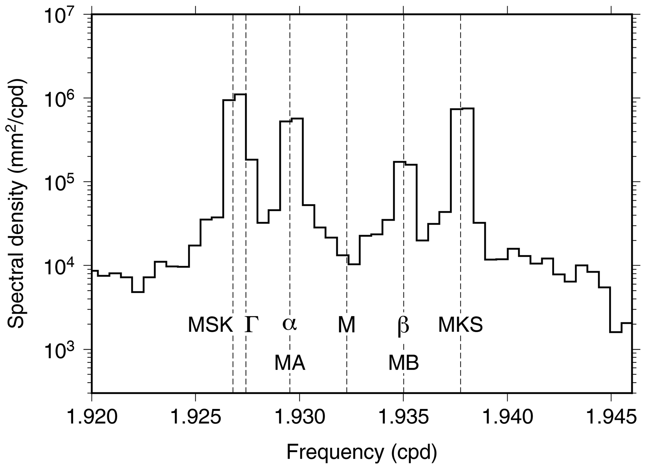
Figure 1 Spectrum of sea level at Saint-Malo, on the northern coast of France, focusing on the M₂ group but with the central M₂ constituent estimated and removed to better delineate the much smaller sidelines. The spectrum is based on 16 years of data. After spectral smoothing, the frequency resolution is approximately 0.2 cpy (or 0.0005 cpd), insufficient to clearly separate MSK₂ from Γ₂. The seasonal modulation of M₂ at Saint-Malo is evidently dominated by the two frictional compound tides, although α₂ is also important – see the discussion in Sect. 3.2.

Table 1 Tidal constituents within the M₂ group.

τ – mean lunar time, h – mean longitude of the Sun, p – mean longitude of lunar perigee, p^′ – mean longitude of solar perigee, currently about 283^∘.

The constituent arguments given in the table are in the form of the standard mean longitudes that Doodson (1921) found so useful for ordering the whole tidal catalog. Simple expressions, linear in time for present-day tides, are readily available to evaluate the longitudes, and thus the tidal arguments, for any particular time (e.g., Pugh and Woodworth, 2014, p. 68).

All the tides of Table 1 differ in frequency from the central M₂ tide by either one or two cycles per year (cpy). They thus act to modulate the amplitude and/or phase of M₂ at those frequencies – the source, at least in spectral terms, of the seasonality of M₂. Most of the tidal arguments differ from M₂ by either ±h or ±2h, so the modulation is tied to the Sun's declination, zero at the equinox; the speed of h is one cycle per tropical year. The two astronomical tides, α₂ and β₂, differ from M₂ by $\pm {\mathrm{\ell }}^{\prime }$, where ${\mathrm{\ell }}^{\prime }=h-p^{\prime }$ is the Sun's mean anomaly, zero at perihelion, so the modulation is tied to the Sun's distance; the speed of ℓ^′ is one cycle per anomalistic year. The astronomical tide Γ₂ also depends on the position of the moon's perigee p. In an average sense, over many years, the contribution from Γ₂ to M₂ seasonality mostly cancels out, because p (period 8.85 years) varies from one year to the next.

The frequencies of Table 1 are given with sufficient precision to show the tiny differences stemming from tropical versus anomalistic years, which are almost identical because the slowly moving p^′ requires 209 centuries to complete one revolution. So the annual pairs MA₂, MB₂ and α₂,β₂ take practically the same frequencies, and either pair may be used in a tidal analysis. However, because their phases differ, the pairs cannot be interchanged; analysis and any subsequent prediction must maintain consistency.

Each class of constituent is now addressed in more detail.

2.1 Astronomical tides

The four gravitational sidelines are all very small, only about 0.3 % of the primary, or smaller. With arguments depending on the mean longitude of the Sun, they evidently arise from the Sun's third-body perturbations of the lunar orbit. In particular, α₂,β₂ arise from what in lunar theory is called the “annual equation”, which refers to an expansion or compaction of the moon's orbit depending on whether the Sun is at perihelion or aphelion, respectively. With a change in the orbital radius there is a corresponding change in the moon's angular velocity and thus longitude. The variation in longitude is given approximately by $-{\mathrm{669}}^{\prime \prime }\sin {\mathrm{\ell }}^{\prime }$ (Brouwer and Clemence, 1961, p. 329). The radial variation is 49cos ℓ^′ km.

Because the ocean cannot support extremely high-Q resonances, the ocean's response (admittance) to gravitational forcing must be nearly constant across the small frequency band of the M₂ group. In that case, the gravitational components of the four sidelines can all be inferred from measurements of the central M₂ primary. Their amplitudes must be in the same proportion as the relative amplitudes of Table 1, and their phases must be nearly identical to the phase of M₂. It may be possible that this rule is violated in locations where large M₂ currents act through nonlinear dissipation to suppress the sidelines; this has been observed to happen for the M₂ nodal sideline (Ku et al., 1985).

Aside from this one exception, the induced seasonal modulations in M₂ from the astronomical sidelines are easily worked out. At a location with mean M₂ amplitude A and phase lag G, the combined elevation of the group is

$$\begin{array}{rl}{\mathit{\zeta }}_{\mathrm{M}}\left(t\right)=& A\left\{\cos (\mathrm{2}\mathit{\tau }-G)\right.\\ & +c_{\mathit{\alpha }}\cos (\mathrm{2}\mathit{\tau }-{\mathrm{\ell }}^{\prime }+\mathit{\pi }-G)\\ & +c_{\mathit{\beta }}\cos (\mathrm{2}\mathit{\tau }+{\mathrm{\ell }}^{\prime }-G)\\ & +\left.c_{\mathit{\delta }}\cos (\mathrm{2}\mathit{\tau }+\mathrm{2}h-G)\right\},\end{array}$$

where c_i are the relative amplitudes from Table 1, and the Γ₂ constituent has been dropped for the reasons noted above. In analogy with the usual approach for handling nodal modulations, this expression may be written as a single modulated wave:

$$\begin{array}{}\text{(1)}& {\mathit{\zeta }}_{\mathrm{M}}\left(t\right)=Af\left(t\right)\cos [\mathrm{2}\mathit{\tau }-G+u(t\left)\right],\end{array}$$

where functions f,u vary throughout the year as periodic functions of h (or ℓ^′). Expanding the trigonometric functions and gathering like terms in cos G and sin G lead to

$$\begin{array}{}\text{(2)}& \begin{array}{rl}f\cos u& =\mathrm{1}-(c_{\mathit{\alpha }}-c_{\mathit{\beta }})\cos {\mathrm{\ell }}^{\prime }+c_{\mathit{\delta }}\cos \mathrm{2}h,\\ f\sin u& =(c_{\mathit{\alpha }}+c_{\mathit{\beta }})\sin {\mathrm{\ell }}^{\prime }+c_{\mathit{\delta }}\sin \mathrm{2}h,\end{array}\end{array}$$

or

$$\begin{array}{}\text{(3)}& f\approx \mathrm{1}-\mathrm{0.00041}\cos {\mathrm{\ell }}^{\prime }+\mathrm{0.00114}\cos \mathrm{2}h\end{array}$$

for the amplitude modulation and

$$\begin{array}{}\text{(4)}& u\approx {\mathrm{0.372}}^{\circ }\sin {\mathrm{\ell }}^{\prime }+{\mathrm{0.065}}^{\circ }\sin \mathrm{2}h\end{array}$$

for the phase modulation. The amplitude modulation is insignificant; because the main coefficients in Eq. (2) cancel, the second term from δ₂ is actually larger than the first term but still very small. For the phase modulation in Eq. (4), the first term peaks at ${\mathrm{\ell }}^{\prime }=\mathrm{90}$^∘, which is early April, and the smaller second term shifts that peak to mid-April. So, the observed phase lag of M₂ (u subtracts from G) takes its minimum value in mid-April and its maximum in mid-September. It is interesting to note that the first term in Eq. (4) is exactly twice the Moon's longitude modulation of ${\mathrm{669}}^{\prime \prime }\sin {\mathrm{\ell }}^{\prime }$, alluded to above as arising from the annual equation in the Sun's perturbation of the lunar orbit (it is twice, because M₂ is semidiurnal).

At most tide gauges, the gravitational components of any seasonal variability in the observed M₂ will thus comprise only a minor part. Observed variability will likely differ significantly from what might be inferred from the M₂ admittance or as modeled by Eqs. (3)–(4). Nonetheless, when only the astronomical modulation is important and the M₂ amplitude is moderately large, a phase modulation of 0.7^∘ is easily seen; an example is given in Sect. 3.1.

2.2 Compound tides

Aside from the two compound tides listed in Table 1, there are possibly others that fall within the M₂ group (Simon, 2013). The most important is OP₂, exactly coinciding with MSK₂, and KO₂, exactly coinciding with M₂. The OP₂ and MSK₂ constituents likely arise from different nonlinear aspects of the hydrodynamics (Parker, 1991), although both are generated in shallow water.

The KO₂ tide is important only when M₂ is anomalously small; it can potentially induce an unusual nodal modulation (relative to the standard M₂ modulation), but it has no bearing on seasonality, with one exception: any seasonal variations in the primary K₁ or O₁ tides would induce seasonality in the compound KO₂, but cases where this is significant relative to M₂ must be rare. The few additional compound tides within the group noted by Simon (2013) are from interactions involving the diurnal S₁, which is normally small and will be ignored. Thus, when nonlinear shallow-water processes are acting sufficiently to produce a noticeable MSK₂ (or OP₂), the main effect of this will be equivalent to semiannual modulations in M₂ amplitude and/or phase.

2.3 Climate-induced modulations

The astronomical sidelines in Table 1 sit at discrete known frequencies. Compound tides are similar, although the number of them can sharply increase in shallow water. In contrast, climate-driven modulations are broadband. Although an annual cycle typically dominates, which is the justification for MA₂, MB₂, one might expect higher harmonics in some cases and also possibly a general smearing of observed spectral lines across the group (e.g., Munk et al., 1965).

Müller et al. (2014), building on an earlier study by Foreman et al. (1995), discussed the case of Victoria (Canada). There was a clear annual modulation in both amplitude and phase of M₂ but with an apparent second harmonic. Multi-year tidal analysis of the Victoria data (not shown) does show energy at the MSK₂ (or OP₂) frequency. Whether this is due to the compound tide(s) or to a true second harmonic below MA₂ is not clear. During tidal analysis it is sometimes possible to separate two constituents of identical frequency by exploiting their different nodal modulations (Parker et al., 1999), but in this case the amplitudes appear too weak to allow it.

The question of frictional compound tides versus higher harmonics of MA₂ and MB₂ is only one instance of the more general, and difficult, problem of deciphering the causes of climate-induced modulations, even when manifested by MA₂ or MB₂ acting alone (e.g., Pugh and Vassie, 1994).

2.4 Nomenclature

The constituent names in Table 1 follow both historical and current international conventions – for the latter, see the table maintained by the Tide, Water Level and Current Working Group of the International Hydrographic Organization (https://iho.int, last access: 17 April 2022). The exception is β₂, which does not (as yet) appear in the working group's table. Godin's 1988 book has the same usage as the IHO; his earlier 1972 book left the smaller lines unlabeled (Godin, 1972, 1988). Regarding β₂, however, it is commonly employed in the Earth tide community (e.g., Hartmann and Wenzel, 1995; Calvo et al., 2016; Ducarme and Schueller, 2018), and β₂ falls into the obvious pattern of using the first four letters of the Greek alphabet for the four astronomical constituents.

The two climate constituents apparently began as MA₂ and Ma₂ (Corkan, 1934). That lost favor, probably because a speaker cannot distinguish the two and also because early computers employed only upper-case letters. MB₂ has been used for decades, at least in British work¹. Amin (1976) still used Ma₂, but by 1983 he too had switched to MB₂.

Not included in Table 1 is the pair, H₁, H₂, for the two annual sidelines, which is starting to appear fairly often in the literature, probably because it is used in a popular open-source software package. The use of H₁ for a semidiurnal wave is certainly an oddity, as the tide community has used an integer subscript to denote tidal species since at least the end of the nineteenth century (Darwin, 1883; Harris, 1895; Cartwright, 1999). It is not clear where the symbol originated. An early (possibly first) use was by Pugh and Vassie (1976). Before that, in a discussion of shallow-water tides, Godin (1972, Table 2.14) used the label “(Horn)” for both sidelines, and he cited a discussion by Horn (1960), although Horn himself left the lines unlabeled. Perhaps “(Horn)” has morphed into H₁, H₂, or the labels merely reflect the argument differences of ±h. An important point, however, is that both Godin and Horn, as well as Pugh and Vassie, were referring to the two climate lines – none of their arguments involved p^′ – whereas the H₁, H₂ in present-day use are substituting for the gravitational tides α₂,β₂, as their arguments do involve p^′. In any event, the use of a wrong subscript should be discouraged.

3 Three examples

In this section an example of M₂ seasonality arising from each of the three categories – gravitation, frictional interaction, and climate processes – is presented. For each tide gauge analyzed, a tidal solution based on a single inversion of many years of data was computed, sufficient to obtain reliable estimates of all constituents in Table 1. Based on an appropriate set of the estimated constituents (different for each category), the implied modulation of M₂ over one year was computed by complex demodulation. This is then compared with results of a second tidal inversion (or rather a set of inversions) in which estimates of M₂ were obtained for every month of the multi-year time series, from which monthly means were then computed. The monthly calculations accounted for the conventional 18.6-year nodal modulation of M₂, but no other modulations. (Standard errors in these monthly means were estimated from the standard deviations for each month, scaled by $\mathrm{1}/\surd n$ for n years of data.)

The goal is to confirm that seasonality of M₂, as delineated by monthly mean estimates of amplitude and phase, can – at least in these cases – be accurately reproduced by the modulations from a particular set of spectral lines. Which lines are in play differ depending on the category of causation.

3.1 Astronomical modulations

It is actually not easy to find good examples of seasonal variability stemming solely from the purely astronomical constituents of Table 1. Any potential case must display fairly constant admittances across the group of gravitational constituents. Yet at most tide gauges one sees perturbations in the admittance or one sees significant amplitudes in the compound tides.

The time series at Port Orford, Oregon, is one of the better examples. Tidal constants estimated from 26 years of data² (1994–2021) are listed in Table 2. The magnitudes of tidal admittances $\left|Z\right|$ are all consistent within error limits, all phases are close, and the compound MSK₂ is very small. Combining the harmonic constants of the three astronomical constituents ${\mathit{\alpha }}_{\mathrm{2}},{\mathit{\beta }}_{\mathrm{2}},{\mathit{\delta }}_{\mathrm{2}}$ implies a seasonal modulation of M₂ given by the solid lines of Fig. 2. These are in good agreement with the monthly mean estimates, aside perhaps for the January amplitude.

The theoretical seasonal modulations, based on Eqs. (3)–(4), are shown as the dashed lines. The solid and dashed lines agree well in phase and less well in amplitude at first glance. However, note that the amplitude vertical axis spans only 1 cm, so in fact the amplitude agreement is also quite good, with all data implying very little amplitude modulation. The small differences in amplitude curves occur because the estimated admittances in Table 2 are not identical, simply due to unavoidable estimation error.

Table 2 Amplitude, Greenwich phase lag, and dimensionless admittance for the M₂ group at Port Orford, Oregon.

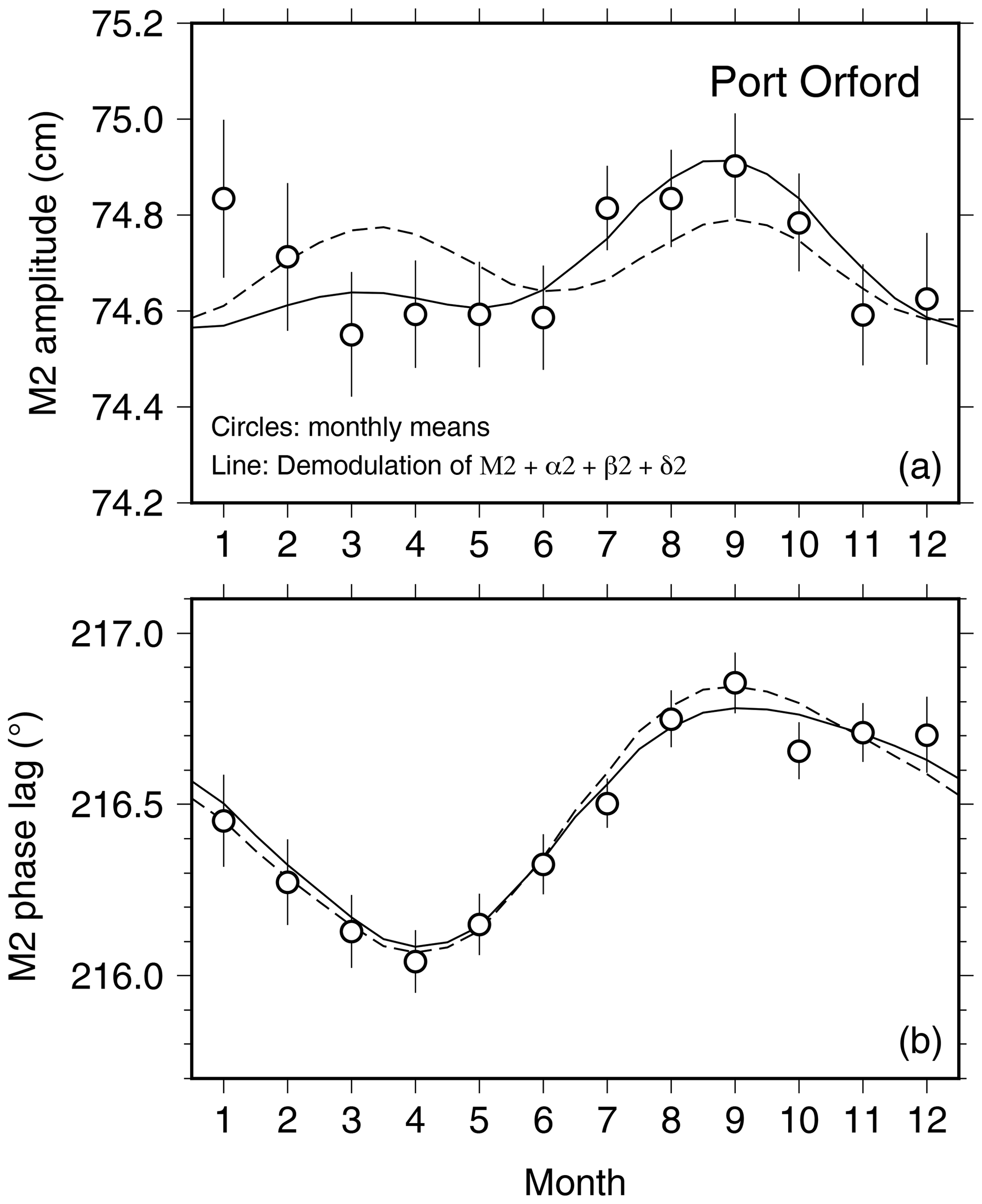
Figure 2 Seasonal variations in M₂ amplitude (a) and Greenwich phase lag (b) observed at Port Orford, Oregon. Circles with error bars are based on monthly mean M₂ estimates from 26 years of hourly data. The solid lines are the implied seasonal variations from the estimated side constituents α₂, β₂, and δ₂. The dashed lines are a theoretical seasonal modulation based on Eqs. (3)–(4). Note that the amplitude axis spans only 1 cm.

The analysis at Port Orford confirms that the astronomically induced seasonal modulation of M₂ results in almost no amplitude modulation and a phase modulation of about 0.7^∘, with a minimum in April and a maximum in September.

3.2 Frictional/advective modulations

An example of modulations dominated by one or both of the compound tides in the M₂ group is Saint-Malo, France, whose spectrum was shown in Fig. 1. The two annual constituents (α₂,β₂ or MA₂, MB₂) are smaller, as the spectrum reveals, but are still too large to ignore. The total modulation, based on four constituents, is shown in Fig. 3. The amplitude clearly reveals the presence of a semiannual modulation, with a slow rise during the beginning of the year and then a rapid decay between July and October. The phase is dominated by the semiannual effect, with an annual contribution responsible for the September phase lag exceeding the earlier peak in March.

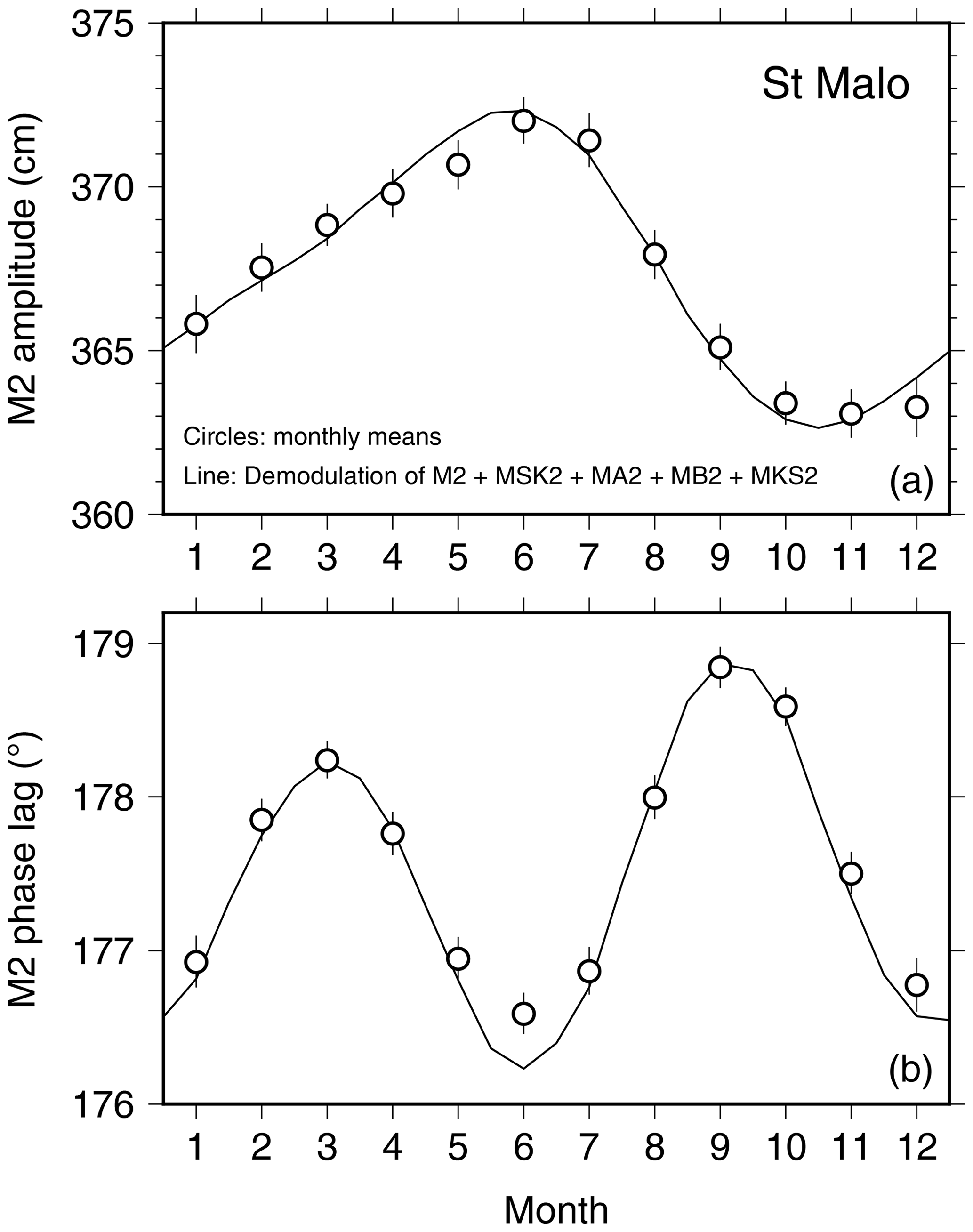
Figure 3 Similar to Fig. 2 but for Saint-Malo, France. The solid line is here based on demodulation of four tidal sidelines, the two annual constituents MA₂, MB₂, and the two compound constituents MSK₂, MKS₂. The latter dominate according to the spectrum shown in Fig. 1 and thus result in the clear semiannual modulation of the M₂ phase.

3.3 Annual climate modulations

Tide gauges with annual variations in M₂, and thus with sidelines dominated by MA₂ and/or MB₂, are easy to find. The case of Victoria was already noted (Müller et al., 2014), partly for having a second harmonic in its modulation. However, there are many tide gauges where only the annual modulation presents itself. A fair number can be found along the coast of Japan, even though M₂ itself is not especially large there. The example chosen here is in fact one of the largest modulations discovered anywhere: Chittagong, along the coast of Bangladesh. At that location the annual sea-level term, Sa, is also anomalously large, presumably reflecting large discharge from the Ganges. Several other nearby tide gauges, with somewhat smaller M₂ modulations, were studied by Tazkia et al. (2017).

Harmonic analysis of 11 years of hourly data (2008–2018) at Chittagong reveals astonishing large amplitudes for MA₂ and MB₂ of 15.5 and 10.1 cm, respectively, with the M₂ constituent at 171.6 cm. The resulting seasonal modulation is shown in Fig. 4. The monthly mean amplitudes range from 146 cm in February to a high of 195 cm in August. In comparison, the phase modulation is not very large, about 4^∘. The monthly mean phases appear slightly erratic and fit the demodulated curve only moderately well.

Figure 4 Similar to Fig. 2 but for Chittagong, along the coast of Bangladesh east of the Ganges Delta. The unusually pronounced modulation of the M₂ amplitude at this location mimics the usually large annual oscillation of sea level, both having a minimum in February and a maximum in July/August.

The large modulation in amplitude at this location closely mimics the large oscillation in annual sea level, which is minimum in February and maximum in July, with a mean range of 71 cm. Tazkia et al. (2017) developed a tide model for the region that explores this interdependence.

4 Conclusions

One indication of the variety of processes responsible for seasonal variability of the M₂ tide is the variety of different mechanisms generating spectral lines within the M₂ group: astronomical motions of the moon, frictional and other nonlinear interactions between tidal waves, and climate processes. The astronomical contribution is predictable given good long-term mean estimates of the M₂ constants; it is mostly a ±0.37^∘ modulation in phase, precisely double the solar perturbation in the moon's longitude arising from the “annual equation” of lunar theory. On the other hand, when a tide gauge is found to be affected by substantial seasonality in M₂, it usually arises from one or both of the constituents MA₂, MB₂. The variety of climate processes responsible for those two constituents – annual changes in stratification, sea level, ice cover, etc. – is where the real complication lies when attempting to understand seasonal variability.