Water masses in the Atlantic Ocean: characteristics and distributions

A large number of water masses are presented in the Atlantic Ocean, and knowledge of their distributions and properties is important for understanding and monitoring of a range of oceanographic phenomena. The characteristics and distributions of water masses in biogeochemical space are useful for, in particular, chemical and biological oceanography to understand the origin and mixing history of water samples. Here, we define the characteristics of the major water masses in the Atlantic Ocean as source water types (SWTs) from their formation areas, and map out their distributions. The SWTs are described by six properties taken from the biased-adjusted Global Ocean Data Analysis Project version 2 (GLODAPv2) data product, including both conservative (conservative temperature and absolute salinity) and non-conservative (oxygen, silicate, phosphate and nitrate) properties. The distributions of these water masses are investigated with the use of the optimum multi-parameter (OMP) method and mapped out. The Atlantic Ocean is divided into four vertical layers by distinct neutral densities and four zonal layers to guide the identification and characterization. The water masses in the upper layer originate from wintertime subduction and are defined as central waters. Below the upper layer, the intermediate layer consists of three main water masses: Antarctic Intermediate Water (AAIW), Subarctic Intermediate Water (SAIW) and Mediterranean Water (MW). The North Atlantic Deep Water (NADW, divided into its upper and lower components) is the dominating water mass in the deep and overflow layer. The origin of both the upper and lower NADW is the Labrador Sea Water (LSW), the Iceland–Scotland Overflow Water (ISOW) and the Denmark Strait Overflow Water (DSOW). The Antarctic Bottom Water (AABW) is the only natural water mass in the bottom layer, and this water mass is redefined as Northeast Atlantic Bottom Water (NEABW) in the north of the Equator due to the change of key properties, especially silicate. Similar with NADW, two additional water masses, Circumpolar Deep Water (CDW) and Weddell Sea Bottom Water (WSBW), are defined in the Weddell Sea region in order to understand the origin of AABW.

1 Introduction

The ocean is composed of a large number of water masses without clear boundaries but gradual transformations between each other (e.g. Castro et al., 1998). Properties of the water in the ocean are not uniformly distributed, and the characteristics vary with regions and depths (or densities). The water masses, which are defined as bodies of water with similar properties and common formation history, are referred to as a body of water with a measurable extent both in the vertical and horizontal directions, and thus it is a quantifiable volume (e.g. Helland-Hansen, 1916, Montgomery, 1958). Mixing occurs inevitably between water masses, both along and across density surfaces, and results in mixtures with different properties away from their formation areas. Understanding of the distributions and variations of water masses has significance for several disciplines of oceanography, for instance, while investigating the thermohaline circulation of the world ocean or predicting climate change (e.g. Haine and Hall, 2002; Tomczak and Godfrey, 2013; Morrison et al., 2015).

The concept of water masses is also important for biogeochemical and biological applications, where the transformations of properties over time can be successfully viewed in the water masses' framework. For instance, the formation of Denmark Strait Overflow Water (DSOW) in the Denmark Strait was described using mixing of a large number of water masses from the Arctic Ocean and the Nordic Seas (Tanhua et al., 2005). A number of investigations show the significance of knowledge about water masses for the biogeochemical oceanography, for instance, the investigation of mineralization of biogenic materials (Alvarez et al., 2014), or the change of ventilation in the oxygen minimum zone (Karstensen et al., 2008). In a more recent work, Garcia-Ibanez et al. (2015) considered 14 water masses combined with velocity fields to estimate transport of water masses, and thus chemical constituents, in the north Atlantic. Similarly, Jullion et al. (2017) used water mass analysis in the Mediterranean Sea to better understand the dynamics of dissolved barium. However, the lack of a unified definition of overview water masses on a basin or global scale leads to additional and repetitive amount of work by redefining water masses in specific regions. The goal of this study is to facilitate water mass analysis in the Atlantic Ocean, and in particular, we aim at supporting biogeochemical and biological oceanographic work in a broad sense.

Understanding the formation, transformation, and circulation of water masses has been a research topic in oceanography since the 1920s (e.g. Jacobsen, 1927; Defant, 1929; Wüst and Defant, 1936; Sverdrup et al., 1942). The early studies were mainly based on (potential) temperature and (practical) salinity as summarized by Emery and Meincke (1986). The limitation of the analysis based on T–S relationship is obvious; distributions of more (than three) water masses cannot be analysed at the same time with only these two parameters, so physical and chemical oceanographers have worked to add more parameters to the characterization of water masses (e.g. Tomczak and Large, 1989; Tomczak, 1981, 1999). The optimum multi-parameter (OMP) method extends the analysis so that more water masses can be considered by adding parameters/water properties (such as phosphate and silicate) and solving the equations of linear mixing without assumptions. The OMP analysis has been successfully applied in a range of studies, for instance, for the analysis of mixing in the thermocline in the eastern Indian Ocean (Poole and Tomczak, 1999).

An accurate definition and characterization is the prerequisite for the analysis of water masses. In this study, the concepts and definitions of water masses given by Tomczak (1999) are used, and we seek to define the key properties of the main water masses in the Atlantic Ocean and to describe their distributions. In order to facilitate the analysis, the Global Ocean Data Analysis Project version 2 (GLODAPv2) data product is used to identify and define the characteristics of the most prominent water masses based on six commonly measured physical and biogeochemical properties (Fig. 1). The water masses are defined in a static sense; i.e. they are assumed to be steady and not change over time, and subtle differences between closely related water masses are not considered in this basin-scale focused study. The so-defined water masses are in a subsequent step used to estimate their distributions in the Atlantic Ocean, again based on the GLODAPv2 data product. Detailed investigations on temporal variability of water masses, or their detailed formation processes, for instance, may find this study useful but will certainly want to use a more granular approach to water mass analysis in their particular areas.

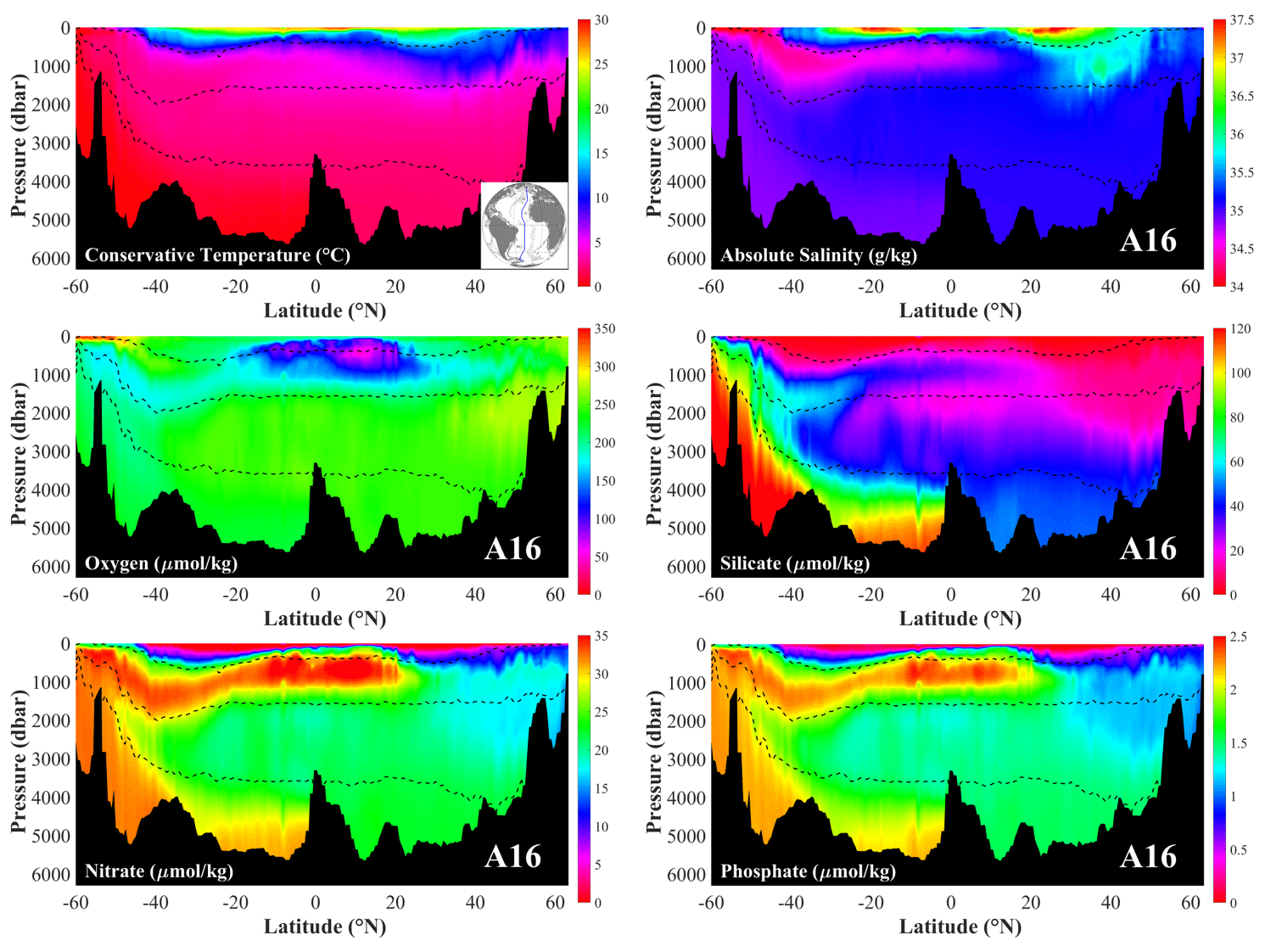
Figure 1 The Atlantic distribution of key properties required by the OMP analysis along the A16 section as occupied in 2013 (expo code: 33RO20130803 in North Atlantic and 33RO20131223 in South Atlantic). The dashed lines show the neutral densities at 27.10, 27.90 and 28.10 kg m⁻³.

2 Data and methods

2.1 The GLODAPv2 data product

Oceanographic surveys conducted by different countries have been actively organized and coordinated since late 1950s. WOCE (the World Ocean Circulation Experiment), JGOFS (Joint Global Ocean Flux Study) and OACES (Ocean Atmosphere Carbon Exchange Study) are three typical representatives of international coordination in the 1990s. The GLODAP data product was devised and implemented in this context with the aim to create a global dataset suitable to describe the distribution and interior ocean inorganic carbon variables (Key et al., 2004, 2010). The first edition (GLODAPv1.1) contains data up to 1999, whereas the updated and expanded version, GLODAPv2 (Key et al., 2015; Olsen et al., 2016), was published in 2016, and the GLODAP team is striving for annual updates (Olsen et al., 2019, 2020). Since GLODAPv2 is a comprehensive and, more importantly, biased-adjusted data product, this is used to quantify the characteristics of water masses. The data in the GLODAPv2 product have passed both a primary quality control (QC), aiming at precision of the data and unity of the units, and a secondary quality control, aiming at the accuracy of the data (Tanhua et al., 2010). The GLODAPv2 data product is adjusted to correct for any biases in data through these QC routines and is unique in its internal consistency and is thus an ideal product to use for this work. Armed with the internally consistent data in GLODAPv2, we utilize previously published studies on water masses and their formation areas to define areas and depth/density ranges that can be considered to be representative samples of water masses.

The variables of absolute salinity (SA in g kg⁻¹), conservative temperature (CT in ^∘C) and neutral density (γ in kg m⁻³), which consider the thermodynamic properties such as entropy, enthalpy and chemical potential (Jackett et al., 2006; Groeskamp et al., 2016), are used in this study because they systematically reflect the spatial variation of seawater composition in the ocean, as well as the impact from dissolved neutral species on the density, and provide a more conservative, actual and accurate description of seawater properties (Millero et al., 2008; Pawlowicz et al., 2011; Nycander et al., 2015).

2.2 Water masses and source water types

In practice, defining properties of water masses (WMs) is often a difficult and time-consuming part, particularly when analysing water masses in a region distant from their formation areas. Tomczak (1999) defined a water mass as “a body of water with a common formation history, having its origin in a particular region of the ocean”, whereas source water types (SWTs) describe “the original properties of water masses in their formation areas”. The distinction between the WMs and SWTs is that WMs define physical extents, i.e. a volume, while SWTs are only mathematical definitions; i.e. SWTs are defined values of properties without physical extents. Knowledge of the SWTs, on the other hand, is essential in labelling WMs, tracking their spreading or mixing progresses, since the values from SWTs describe their initial characteristics and can be considered as the fingerprints of WMs. The SWT of a WM is defined by the values of key properties, while some of them, like central waters, require more than one SWT to be defined (Tomczak, 1999). In this study, the terminology “water mass” is used in the discussions, realizing that the properties of the WMs used for the further analysis actually refer to SWTs.

2.3 OMP analysis

2.3.1 Principle of OMP analysis

For the analysis, six key properties are used to define SWTs, including two conservative (CT and SA) and four non-conservative (oxygen, silicate, phosphate and nitrate) properties. In order to determine the distributions of WMs, the OMP analysis is invoked as objective mathematical formulations of the influence of mixing (Karstensen and Tomczak, 1997, 1998). The starting point is the six key properties (Fig. 1) from observations (such as CT_obs is the observed conservative temperature). The OMP model determines the contributions from predefined SWTs (such as CT_i that describes the conservative temperature in each SWT), which represent the values of the “unmixed” WMs in the formation areas, through a linear set of mixing equations, assuming that all key properties of water masses are affected similarly by the same mixing processes. The fractions (x_i) in each sampling point are obtained by finding the best linear mixing combination in parameter space defined by six key properties and minimizing the residuals (R, such as R_CT is the residual of conservative temperature) in a non-negative least-squares sense (Lawson and Hanson, 1974) as shown in the following equations:

$$\begin{array}{}\text{(1)}& {\displaystyle }{x}_{\mathrm{1}}{\mathrm{CT}}_{\mathrm{1}}+x_{\mathrm{2}}{\mathrm{CT}}_{\mathrm{2}}+\mathrm{\dots }+x_n{\mathrm{CT}}_n={\mathrm{CT}}_{\mathrm{obs}}+R_{\mathrm{CT}}\text{(2)}& {\displaystyle }{x}_{\mathrm{1}}{\mathrm{SA}}_{\mathrm{1}}+x_{\mathrm{2}}{\mathrm{SA}}_{\mathrm{2}}+\mathrm{\dots }+x_n{\mathrm{SA}}_n={\mathrm{SA}}_{\mathrm{obs}}+R_{\mathrm{SA}}\text{(3)}& {\displaystyle }{x}_{\mathrm{1}}{\mathrm{O}}_{\mathrm{1}}+x_{\mathrm{2}}{\mathrm{O}}_{\mathrm{2}}+\mathrm{\dots }+x_n{\mathrm{O}}_n={\mathrm{O}}_{\mathrm{obs}}+R_{\mathrm{O}}\text{(4)}& {\displaystyle }{x}_{\mathrm{1}}{\mathrm{Si}}_{\mathrm{1}}+x_{\mathrm{2}}{\mathrm{Si}}_{\mathrm{2}}+\mathrm{\dots }+x_n{\mathrm{Si}}_n={\mathrm{Si}}_{\mathrm{obs}}+R_{\mathrm{Si}}\text{(5)}& {\displaystyle }{x}_{\mathrm{1}}{\mathrm{Ph}}_{\mathrm{1}}+x_{\mathrm{2}}{\mathrm{Ph}}_{\mathrm{2}}+\mathrm{\dots }+x_n{\mathrm{Ph}}_n={\mathrm{Ph}}_{\mathrm{obs}}+R_{\mathrm{Ph}}\text{(6)}& {\displaystyle }{x}_{\mathrm{1}}{\mathrm{N}}_{\mathrm{1}}+x_{\mathrm{2}}{\mathrm{N}}_{\mathrm{2}}+\mathrm{\dots }+x_n{\mathrm{N}}_n={\mathrm{N}}_{\mathrm{obs}}+R_{\mathrm{N}}\text{(7)}& {\displaystyle }{x}_{\mathrm{1}}+x_{\mathrm{2}}+\mathrm{\dots }+x_n=\mathrm{1}+R,\end{array}$$

where the CT_obs, SA_obs, O_obs, Si_obs, Ph_obs and N_obs are the observed values of properties; CT_i, SA_i, O_i, Si_i, Ph_i and N_i (i=1, 2 …, n) represent the predetermined (known) values in each SWT for each property. The last row expresses the condition of mass conservation.

OMP analysis represents an inversion of an overdetermined system in each sampling point, so that the sampling points are required to be located “downstream” from the formation areas, i.e. on the spreading pathway. The total number of WMs which can be analysed simultaneously within one OMP run is limited by the number of variables/key properties, because mathematically, six variables (x₁–x₆) can be solved with six equations. In our analysis, one OMP run can solve up to six WMs. The above system of equations can be written in matrix notation as

$$\begin{array}{}\text{(8)}& G\cdot x-d=R,\end{array}$$

where G is a parameter matrix of defined SWTs with six key properties, x is a vector containing the relative contributions from the “unmixed” water masses to the sample (i.e. solution vector of the SWT fractions), d is a data vector of water samples (observational data from GLODAPv2 in this study) and R is a vector of residual. The solution is to find the minimum of the residual (R) with a linear fit of parameters (key properties) for each data point with a non-negative values. In this study, the mixed layer is not considered, as its properties tend to be strongly variable on seasonal timescales so that water mass analysis is inapplicable. The solution is dependent on, and sensitive to, the prior assumptions of the properties of the SWTs. Here, we have not explicitly explored this sensitivity but note that a common difficulty in OMP analysis is to properly define the SWT properties, and that this study provides a generally applicable set of SWT properties for the major water masses in the Atlantic Ocean.

2.3.2 Extended OMP analysis

The prerequisite (or restriction) for using (basic) OMP analysis is that the water masses are formed close enough to the water samples with short transport times within a limited ocean region, for instance, an oceanic front or intertidal belt, so that the mixing can be assumed not to be influenced by biogeochemical processes (i.e. assume all the parameters to be quasi-conservative). However, biogeochemical processes cannot be ignored in a basin-scale analysis (Karstensen and Tomczak, 1998). Obviously, this prerequisite does not apply to our investigation for the entire Atlantic, so the “extended” OMP analysis is required. In this concept, non-conservative parameters (phosphate and nitrate) are converted into conservative parameters by introducing the “preformed” nutrients PO and NO, where PO and NO denote the concentrations of phosphate and nitrate in seawater by considering the consumption of dissolved oxygen by respiration (in other words, the alteration due to respiration is eliminated) (Broecker, 1974; Karstensen and Tomczak, 1998). In addition, a new column should be added to the equations for non-conservative properties (aΔO₂, aΔSi, aΔPh and aΔN) to express the changes in SWTs due to biogeochemical impacts, namely, the change of oxygen concentration with the remineralization of nutrients:

$$\begin{array}{}\text{(9)}& {\displaystyle }{x}_{\mathrm{1}}{\mathrm{CT}}_{\mathrm{1}}+x_{\mathrm{2}}{\mathrm{CT}}_{\mathrm{2}}+\mathrm{\dots }+x_n{\mathrm{CT}}_n={\mathrm{CT}}_{\mathrm{obs}}+R_{\mathrm{CT}}\text{(10)}& {\displaystyle }{x}_{\mathrm{1}}{\mathrm{SA}}_{\mathrm{1}}+x_{\mathrm{2}}{\mathrm{SA}}_{\mathrm{2}}+\mathrm{\dots }+x_n{\mathrm{SA}}_n={\mathrm{SA}}_{\mathrm{obs}}+R_{SA}\text{(11)}& {\displaystyle }{x}_{\mathrm{1}}{\mathrm{O}}_{\mathrm{1}}+x_{\mathrm{2}}{\mathrm{O}}_{\mathrm{2}}+\mathrm{\dots }+x_n{\mathrm{O}}_n-a\mathrm{\Delta }{\mathrm{O}}_{\mathrm{2}}={\mathrm{O}}_{\mathrm{obs}}+R_{\mathrm{O}}\text{(12)}& {\displaystyle }{x}_{\mathrm{1}}{\mathrm{Si}}_{\mathrm{1}}+x_{\mathrm{2}}{\mathrm{Si}}_{\mathrm{2}}+\mathrm{\dots }+x_n{\mathrm{Si}}_n+a\mathrm{\Delta }\mathrm{Si}={\mathrm{Si}}_{\mathrm{obs}}+R_{\mathrm{Si}}\text{(13)}& {\displaystyle }{x}_{\mathrm{1}}{\mathrm{Ph}}_{\mathrm{1}}+x_{\mathrm{2}}{\mathrm{Ph}}_{\mathrm{2}}+\mathrm{\dots }+x_n{\mathrm{Ph}}_n+a\mathrm{\Delta }\mathrm{Ph}={\mathrm{Ph}}_{\mathrm{obs}}+R_{\mathrm{Ph}}\text{(14)}& {\displaystyle }{x}_{\mathrm{1}}{\mathrm{N}}_{\mathrm{1}}+x_{\mathrm{2}}{\mathrm{N}}_{\mathrm{2}}+\mathrm{\dots }+x_n{\mathrm{N}}_n+a\mathrm{\Delta }\mathrm{N}={\mathrm{N}}_{\mathrm{obs}}+R_{\mathrm{N}}\text{(15)}& {\displaystyle }{x}_{\mathrm{1}}+x_{\mathrm{2}}+\mathrm{\dots }+x_n=\mathrm{1}+R.\end{array}$$

As a result, the number of water masses should be further reduced in one OMP run if the biogeochemical processes are considered and extended OMP analysis is used. In this study, the total number of five water masses is included in each OMP run.

2.3.3 Presence of mass residual

The fractions of WMs in each sample are obtained by finding the best linear mixing combination in parameter space defined by six key properties which minimizes the residuals (R) in a non-negative least-squares sense. Ideally, a value of 100 % is expected when the fractions of all the water masses are added together. However, mass residuals, where the sum of water masses for a sample differs from 100 %, are inevitable during the analysis and are due to sample properties outside the input SWTs to the OMP formulation. There are two different cases. The first is that a single water mass is larger than 100 % and other water masses are all 0 %. This mostly happens in the central waters (γ<27.10 kg m⁻³, Fig. 2). The reason is that key properties, for instance, CT, of central waters are variable. When the CT increases beyond the range of this water mass, the OMP analysis considers the fraction is over 100 %. In this case, all such samples are set to 100 % after confirming the absence of any other water mass. The second case is that none of the individuals water masses are more than 100 %, but the total fraction is more than 100 % when added together. In this study, the total fractions are generally less than 105 % (γ>27.10 kg m⁻³; Fig. 2).

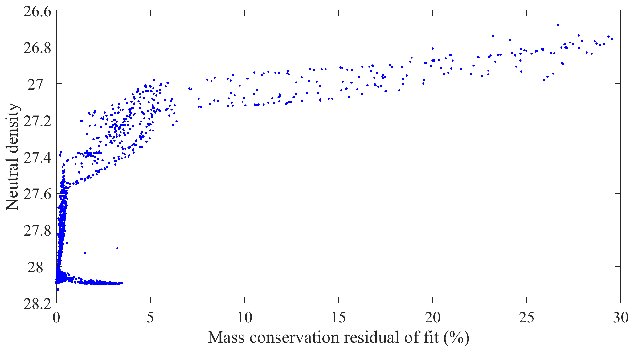
Figure 2 An example of a mass conservation residual in OMP analysis for the A03 section. This figure indicates that in density layers outside of the water masses included in the analysis, we find a high residual; i.e. the OMP analysis should only be used for a certain density interval.

In order to map the distributions of water masses, all GLODAPv2 data in the Atlantic Ocean (below the mixed layer) are analysed with the OMP method by using six key properties. In order to solve the contradiction between the limitation of water masses in one OMP run and the total number of 16 water masses (Fig. 3), the Atlantic Ocean is divided into 17 regions (Table 1) and each with its own OMP formulation, by only including water masses that are likely to appear in the area. In the vertical, neutral density intervals are used to separate boxes. In the horizontal direction, the division lines are 40^∘ N, the Equator and 50^∘ S, where the area south of 50^∘ S is one region, independent of density, and additional divisions are set between the Equator and 40^∘ N (γ at 26.70 and 27.30 kg m⁻³, latitude of 30^∘ N; Table 1). In this way, we end up with a set of 17 different OMP formulations that are used for estimating the fraction(s) of water masses in each water sample. The neutral density and the latitude of the water sample are thus used to determine which OMP should be applied (Table 1). Note that all water masses are present in more than one OMP so that reasonable (i.e. smooth) transitions between the different areas can be realized.

Table 1 Schematic of the selection criteria for the OMP analysis (runs) in this study.

Figure 3 T–S diagram of all Atlantic data from the GLODAPv2 data product (grey dots) indicating the 16 main SWTs in the Atlantic Ocean discussed in this study. The coloured dots with letters A–D show the upper and lower boundaries of central waters, and E–P show the mean values of other SWTs.

3 Overview of the water masses in the Atlantic Ocean and the criteria of selection

In line with the results from Emery and Meincke (1986) and from our interpretation of the observational data from GLODAPv2, the water masses in the Atlantic Ocean are considered to be distributed in four main isopycnal (vertical) layers separated by surfaces of equal (neutral) density (Fig. 4). The upper (shallowest) layer with lowest neutral density is located within the upper ∼ 500–1000 m of the water column (below the mixed layer and γ<27.10 kg m⁻³). The intermediate layer is located between ∼ 1000 and 2000 m (γ between 27.10 and 27.90 kg m⁻³). The deep and overflow layer occupies the layer between ∼ 2000–4000 m (γ between 27.90 and 28.10 kg m⁻³), whereas the bottom layer is the deepest layer and mostly located below ∼ 4000 m (γ>28.10 kg m⁻³).

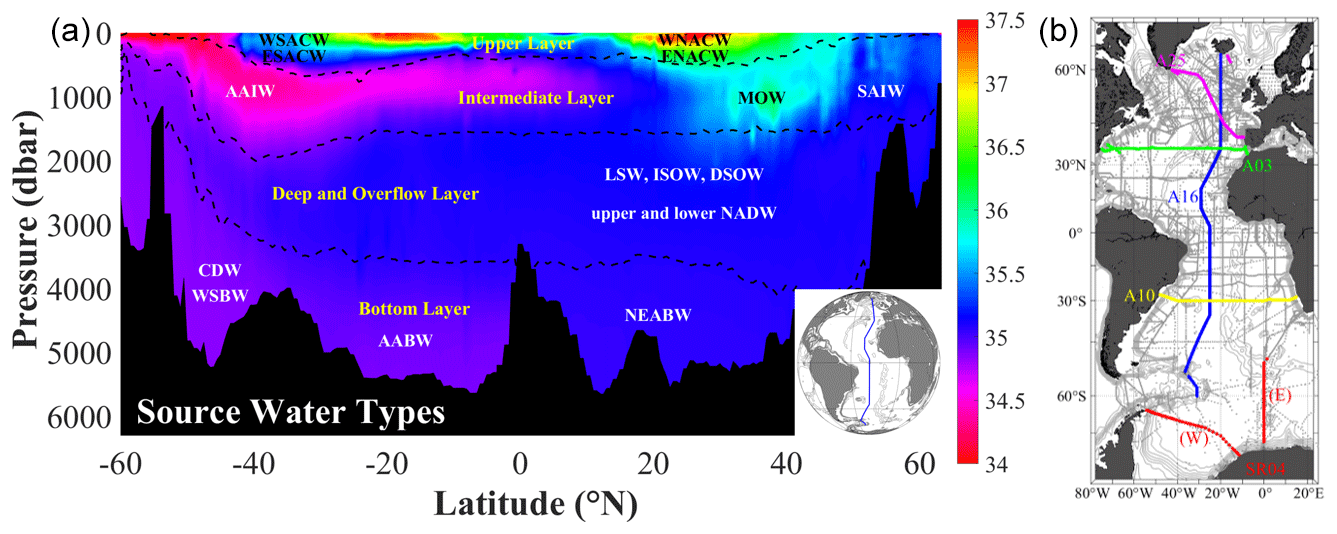
Figure 4 (a) Distributions of water masses in the Atlantic Ocean based on the A16 section in 2013. The background colour shows the absolute salinity (g kg⁻¹). The dashed lines show the boundary of the four vertical layers divided by neutral density. (b) Five selected WOCE/GO-SHIP sections that were selected in this work to represent the vertical distribution of the main water masses.

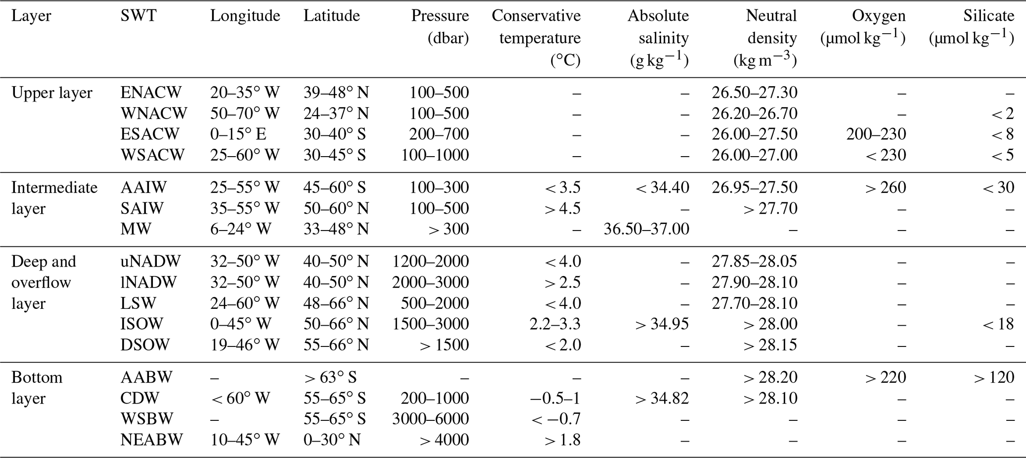
To define the main water masses in the Atlantic Ocean, the determination of their formation areas is the first step (Fig. 5), and then the selection criteria are listed to define SWTs based on the CT–SA distribution, pressure (P) or neutral density (γ) (Table 2). See Table 3 for the abbreviations of the water mass names. For some SWTs, additional properties such as oxygen or silicate are also required for the definition. With these criteria, which are taken from the literature and also based on data from GLODAPv2 product, the SWTs of all the main water masses can be defined for further estimating their distributions in the Atlantic Ocean by using OMP analysis.

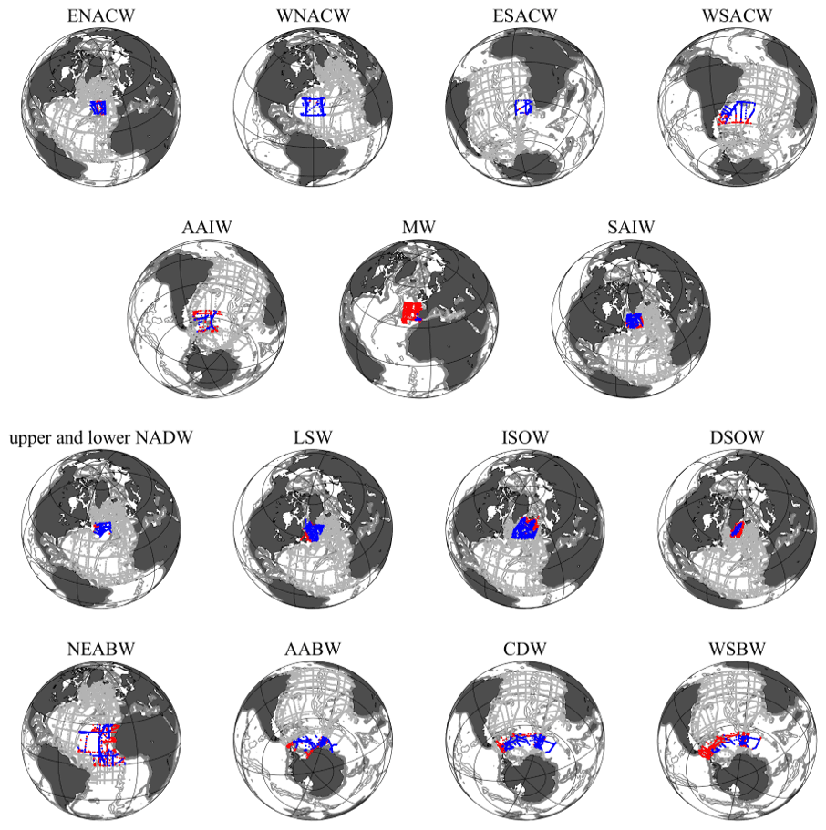
Figure 5 Formation/redefining areas of the 16 main water masses in the Atlantic Ocean. The red dots show stations in formation area, the blue dots show stations where the SWT was found, and the grey dots show all the stations from the GLODAPv2 dataset.

For the water masses in the upper layer, i.e. the central waters, properties cover a “wide” range instead of a “narrow” point value due to their variations, especially in CT and SA space; i.e. the central waters are labelled by two SWTs to identify the upper and lower boundaries of properties (Karstensen and Tomczak, 1997, 1998). In order to determine these two SWTs, one property is taken as a benchmark (neutral density in this investigation) and the relationships to the others are plotted to make a linear fit, and the two endpoints are selected as SWTs to label central waters (Fig. 6).

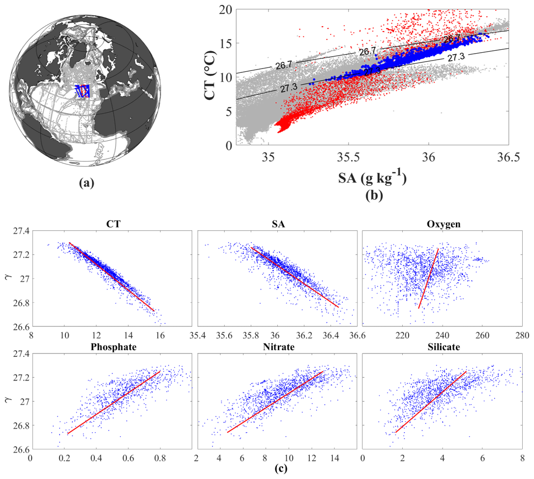
Figure 6 Example of a selection of water samples to define a water mass (here ENACW): (a) the formation area, (b) the T–S diagram. The red dots show all the data in formation area, the blue dots show the selected data as ENACW, and the grey dots show all the data from the GLODAPv2 dataset. (c) Six key properties vs. neutral density (γ) as independent variable. Blue dots show the selected data as ENACW from panels (a) and (b), and the red line shows the linear fit. The start and end points of the red line are the upper and lower boundaries of ENACW.

During the determination of each SWT, two figures are displayed to characterize them, including (a) depth profiles of the six key properties under consideration (same colour coding), and (b) bar plots from the distributions of the samples within the criteria (the blue dots in Figs. 6 and 7) for a SWT with a Gaussian curve to show the statistics (Fig. 7). The plots of properties vs. pressure provide an intuitive understanding of each SWT compared to other WMs in the region. The distributions of properties with the Gaussian curves are the basis to visually determine and confirm the SWT property values and associated standard deviations.

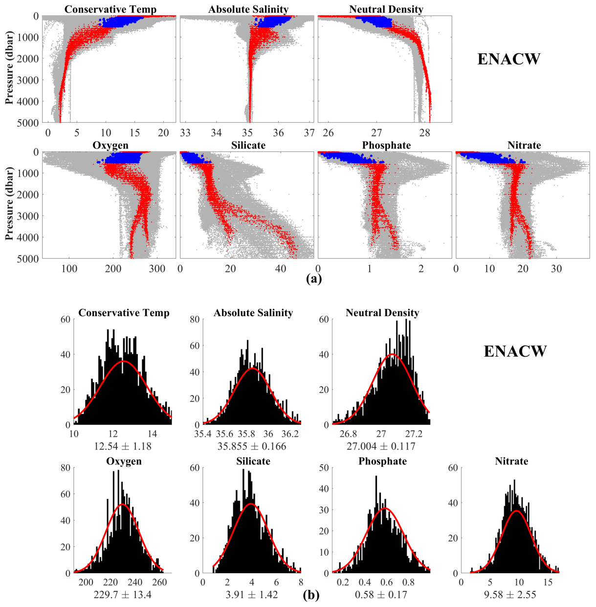
Figure 7 Example of the definition of an SWT (here ENACW): (a) the distribution of key properties vs. pressure; (b) bar plots of the data distribution of samples used to define the SWTs: conservative temperature (^∘C), absolute salinity (g kg⁻¹), neutral density (kg m⁻³), oxygen and nutrients (µmol kg⁻¹). The red Gaussian fit shows mean value and standard deviation of selected data.

Most water masses maintain their original characteristics away from their formation areas. However, some are worthy of mention as products from mixing of several original water masses (for instance, North Atlantic Deep Water is the product of Labrador Sea Water, Iceland–Scotland Overflow Water and DSOW). Also, characteristics of some water masses change sharply during their pathways (namely, the sharp drop silicate concentration of Antarctic Bottom Water after passing the Equator). As a result, it is advantageous to redefine their SWTs. In order to distinguish such water masses from the other original ones, their defined specific areas are mentioned as “redefining” areas instead of formation areas, because, strictly speaking, they are not “formed” in these areas. The calculated water mass fractions for the Atlantic Ocean data in GLODAPv2 are available at https://www.ncei.noaa.gov/access/ocean-carbon-data-system/oceans/ndp_107/ndp107.html, last access: 5 March 2021.

Table 2 Summary of the criteria used to select the water samples considered to represent the source water types discerned in this study. For convenience, they are grouped into four depth layers.

4 The upper layer, central waters

The upper layer is occupied by four central waters known to be formed by winter subduction with upper and lower boundaries of properties. All values between these boundaries are used to calculate the means and standard deviations (Figs. 7 and S1–S3), and it occupies two SWTs in one OMP run.

Central waters can be easily recognized by their linear CT–SA relationships (Pollard et al., 1996; Stramma and England, 1999). In this study, the upper layer is defined to be located above the neutral density isoline of 27.10 kg m⁻³ (below the mixed layer). The formations and transport of the central waters are influenced by the currents in the upper layer and finally form relative distinct bodies of water in both the horizontal and vertical directions (Fig. 8). The concept of mode water is referred to as the subregions of central water, which describes the particularly uniform properties of seawater within the upper layer and more refers to the physical properties (such as the CT–SA relationship and potential vorticity). In this study, the unified name “central water”, which refers more to the biogeochemical properties (Cianca et al., 2009; Alvarez et al., 2014), is used to avoid possible confusion.

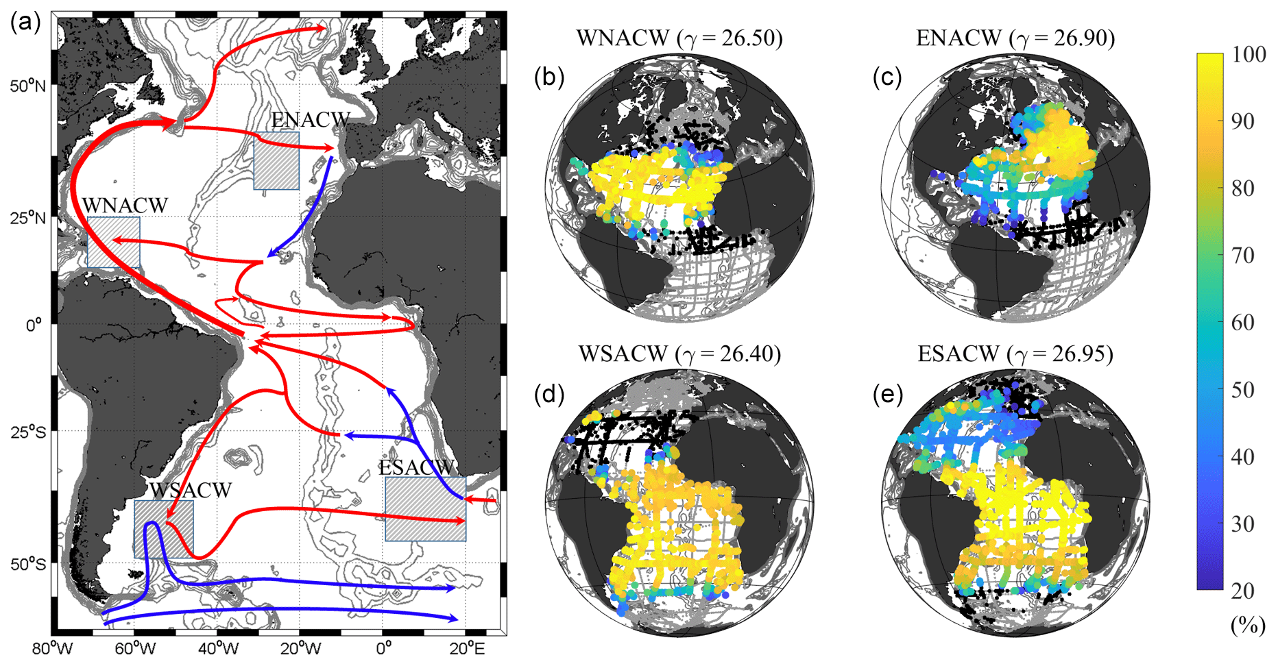
Figure 8 Currents (a) and water masses (b, c, d, e) in the upper layer. (a) The warm (red) and cold (blue) currents (arrows) and the formation areas (rectangular shadows) of water masses in the upper layer. (b, c, d, e) The coloured dots show fractions from 20 % to 100 % of water masses in each station around its core neutral densities (kg m⁻³). Stations with fractions less than 20 % are marked by black dots, while grey dots show all the GLODAPv2 stations.

4.1 Eastern North Atlantic Central Water

The main central water in the region east of the Mid-Atlantic Ridge (MAR) is the Eastern North Atlantic Central Water (ENACW; Harvey, 1982). This water mass is formed in the inter-gyre region during the winter subduction (Pollard and Pu, 1985). One component of the Subpolar Mode Water (SPMW) is carried south and contributes to the properties of ENACW (McCartney and Talley, 1982). The inter-gyre region, limited by latitudes between 39 and 48^∘ N and longitudes between 20 and 35^∘ W (Pollard et al., 1996), is considered as the formation area of ENACW (Fig. 5). Neutral densities of 26.50 and 27.30 kg m⁻³ are selected as the upper and lower boundaries to define the SWT of ENACW (Cianca et al., 2009; Prieto et al., 2015), which is in contrast to Garcia-Ibanez et al. (2015) who used potential temperature (θ) as the upper limit. The core of ENACW is located within the upper 500 m of the water column (Fig. 7a) with the iconic linear T–S relationship (Fig. 6b), consistent with Pollard et al. (1996). The main characteristic of ENACW is the large ranges of temperature and salinity and low nutrient concentrations, especially silicate (Fig. 7b).

4.2 Western North Atlantic Central Water

Western North Atlantic Central Water (WNACW) is another water mass formed through winter subduction (Worthington, 1959; McCartney and Talley, 1982) with the formation area at the southern flank of the Gulf Stream (Klein and Hogg, 1996). In some studies, this water mass is referred to as 18 ^∘C water since a temperature of around 18 ^∘C is one symbolic feature (e.g. Talley and Raymer, 1982; Klein and Hogg, 1996). In general, seawater in the Northeast Atlantic has higher salinity than that in the Northwest Atlantic due to the stronger winter convection (Pollard and Pu, 1985) and input of Mediterranean Water (MW) (Pollard et al., 1996; Prieto et al., 2015). However, for the central waters, the situation is the opposite. WNACW has a significantly higher salinity (SA) (by ∼ 0.9 g kg⁻¹) than ENACW (Table 4). In this study, the work of McCartney and Talley (1982) is followed, and the region of 24–37^∘ N, 50–70^∘ W, at shallower depths than 500 m, is considered as the formation area (Fig. 5). By defining the SWT of WNACW, neutral density between 26.20 and 26.70 kg m⁻³ is selected due to the discrete CT–SA distribution outside this range (Table 2). Besides the linear CT–SA relationship, another property of this water mass is, as the alternative name suggests, a temperature of around 18 ^∘C, which is the warmest in the four central waters due to the low latitude of the formation area and the impact from the warm Gulf Stream (Cianca et al., 2009; Prieto et al., 2015). In addition, the low nutrient concentration is also a significant property compared to other central waters (Fig. S1).

Table 3 The full names of the water masses discussed in this study, and the abbreviations.

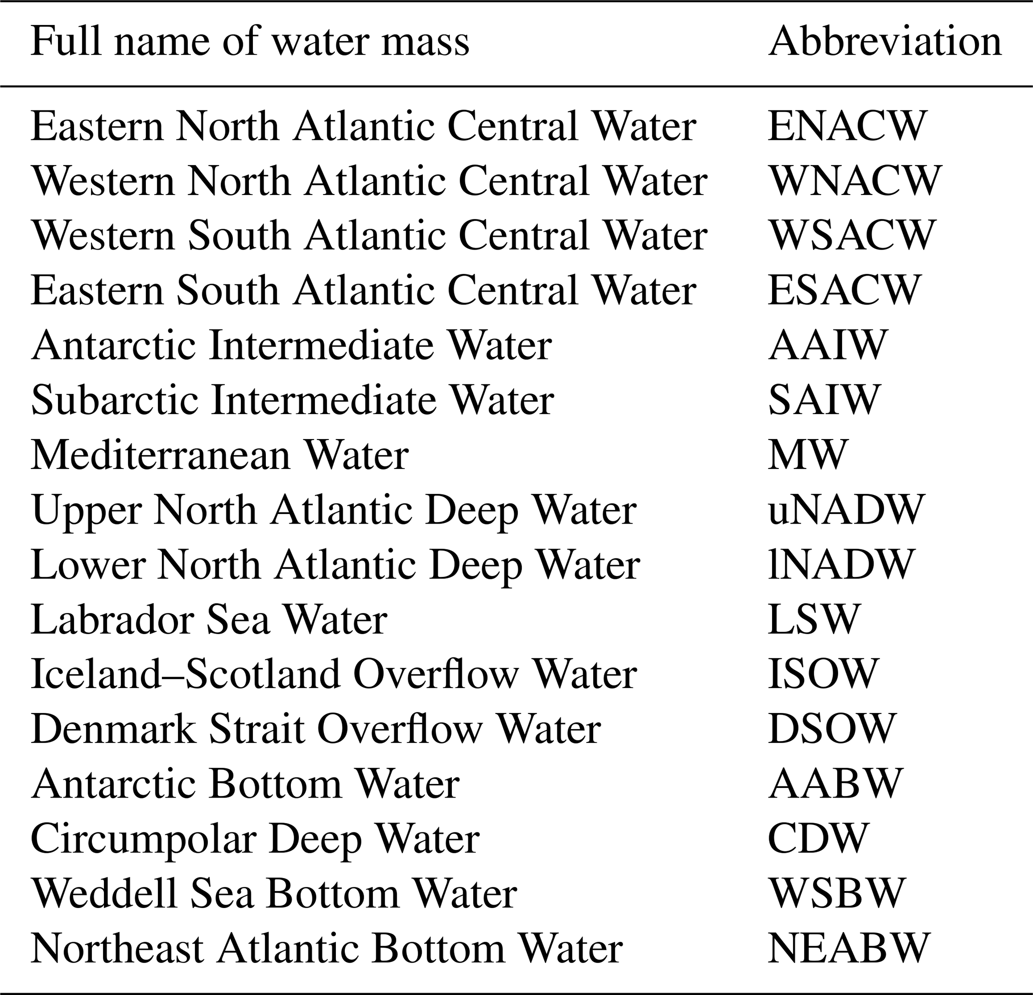
Table 4 Table of the mean value and the standard deviation of all variables for all the water masses (i.e. source water types) in this study.

4.3 Eastern South Atlantic Central Water

The formation area of Eastern South Atlantic Central Water (ESACW) is located in area southwest of South Africa and south of the Benguela Current (Peterson and Stramma, 1991). In this region, the Agulhas Current brings water from the Indian Ocean (Deruijter, 1982; Lutjeharms and van Ballegooyen, 1988) that mixes with the South Atlantic Current from the west (Stramma and Peterson, 1990; Gordon et al., 1992). The origin of ESACW can partly be tracked back to the Western South Atlantic Central Water (WSACW) but defined as a new SWT since seawater from Indian Ocean is added by the Agulhas Current. The mixing region of Agulhas Current and South Atlantic Current (30–40^∘ S, 0–20^∘ E) is selected as the formation area of ESACW (Fig. 5). To investigate the properties of ESACW, results from Stramma and England (1999) are followed, and we consider 200–700 m as the core of this water mass. For the properties, neutral density (γ) between 26.00 and 27.00 kg m⁻³ and oxygen concentration higher than 230 µmol kg⁻¹ are used to define ESACW (Table 2). Similar to ENACW, ESACW also exhibits relative large CT and SA ranges and low nutrient concentrations (especially low in silicate) compared to the AAIW below. The properties of ESACW are similar to those of WSACW, although with higher nutrient concentrations due to input from the Agulhas Current (Fig. S2).

4.4 Western South Atlantic Central Water

The WSACW is formed in the region near the South American coast between 30 and 45^∘ S, where surface South Atlantic Current brings central water to the east (Kuhlbrodt et al., 2007). The WSACW is formed with little direct influence from other CW masses (Sprintall and Tomczak, 1993; Stramma and England, 1999), while the origin of other central waters (e.g. ESACW or ENACW) can be traced back, to some extent at least, to WSACW (Peterson and Stramma, 1991). This water mass is a product of three mode waters mixed together: the Brazil Current brings salinity maximum water (SMW) and Subtropical Mode Water (STMW) from the north, while the Falkland Current brings Subantarctic Mode Water (SAMW) from the south (Alvarez et al., 2014). Here, we follow the work of Stramma and England (1999) and Alvarez et al. (2014) and choose the meeting region of these two currents (30–45^∘ S, 25–60^∘ W) as the formation area of WSACW (Fig. 5). Neutral density (γ) between 26.0 and 27.0 kg m⁻³ is selected to define the SWT of WSACW, and the requirement of silicate concentrations lower than 5 µmol kg⁻¹ and oxygen concentrations lower than 230 µmol kg⁻¹ is also added (Table 2). WSACW shows similar hydrochemical properties to other central waters such as a linear T–S relationship with large T and S ranges and low concentration of nutrients, especially silicate (Fig. S3).

4.5 Atlantic distribution of central waters

Based on the OMP analysis of the GLODAPv2 data product, the physical extent of the central waters can be described over the Atlantic Ocean. The horizontal distributions of four central waters in the upper layer are shown on the maps in Fig. 8, and the vertical distributions along selected GO-SHIP sections are found in Fig. 9. Note that the central waters are found at different densities, with the eastern variations being denser, so there is significant overlap in the horizontal distribution. The vertical extent of the central waters is clearly seen in Fig. 9.

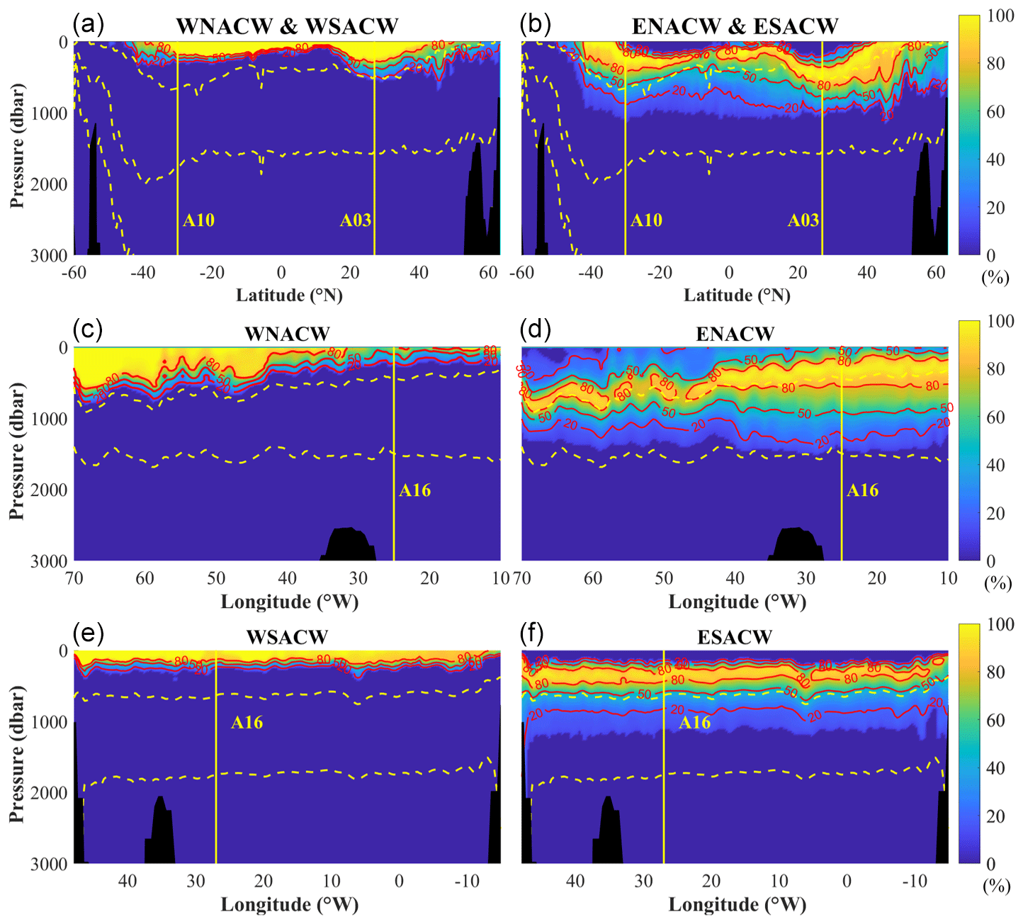
Figure 9 Distribution of central water masses based on A16 (a, b), A03 (c, d), and A10 (e, f) sections for the top 3000 m depth. The contour lines show fractions of 20 %, 50 % and 80 %, yellow vertical lines show cross overs with other sections, and dashed yellow lines show vertical boundaries of layers (neutral density at 27.10, 27.90 and 28.10 kg m⁻³).

ENACW is mainly found in the northeast part of North Atlantic, near the formation area in the inter-gyre region (Fig. 8). High fractions of ENACW are also found in a band across the Atlantic at around 40^∘ N, where the core of this water mass is found at close to 1000 m depth in the western part of the basin (Fig. 9).

WNACW is predominantly found in the western basin of the North Atlantic in a zonal band between ∼ 10 and 40^∘ N (Fig. 8). The vertical extent of WNACW is significantly higher in the western basin with an extent of about 500 m in the west, tapering off towards the east (Fig. 9).

ESACW is found over most of the South Atlantic, as well as in the tropical and subtropical north Atlantic (Fig. 8). The extent of ESACW does reach particularly far north in the eastern part of the basin, where it is an important component over the eastern tropical North Atlantic oxygen minimum zone, roughly south of the Cabo Verde islands. In the vertical direction, the ESACW is located below WSACW (Fig. 9).

The horizontal distribution of WSACW does reach into the Northern Hemisphere but is, obviously, concentrated in the western basin (Fig. 8). In the vertical scale, the WSACW also tends to dominate the upper layer of the South Atlantic above the ESACW (Fig. 9).

5 The intermediate layer

The intermediate water masses have an origin in the upper 500 m of the ocean and subduct into the intermediate depth (1000–1500 m) during their formation process. Similar to the central waters, the distributions of the intermediate waters are significantly influenced by the major currents (Fig. 10a). The neutral density (γ) of the intermediate waters is in general between 27.10 and 27.90 kg m⁻³ and selected as the definition of intermediate layer.

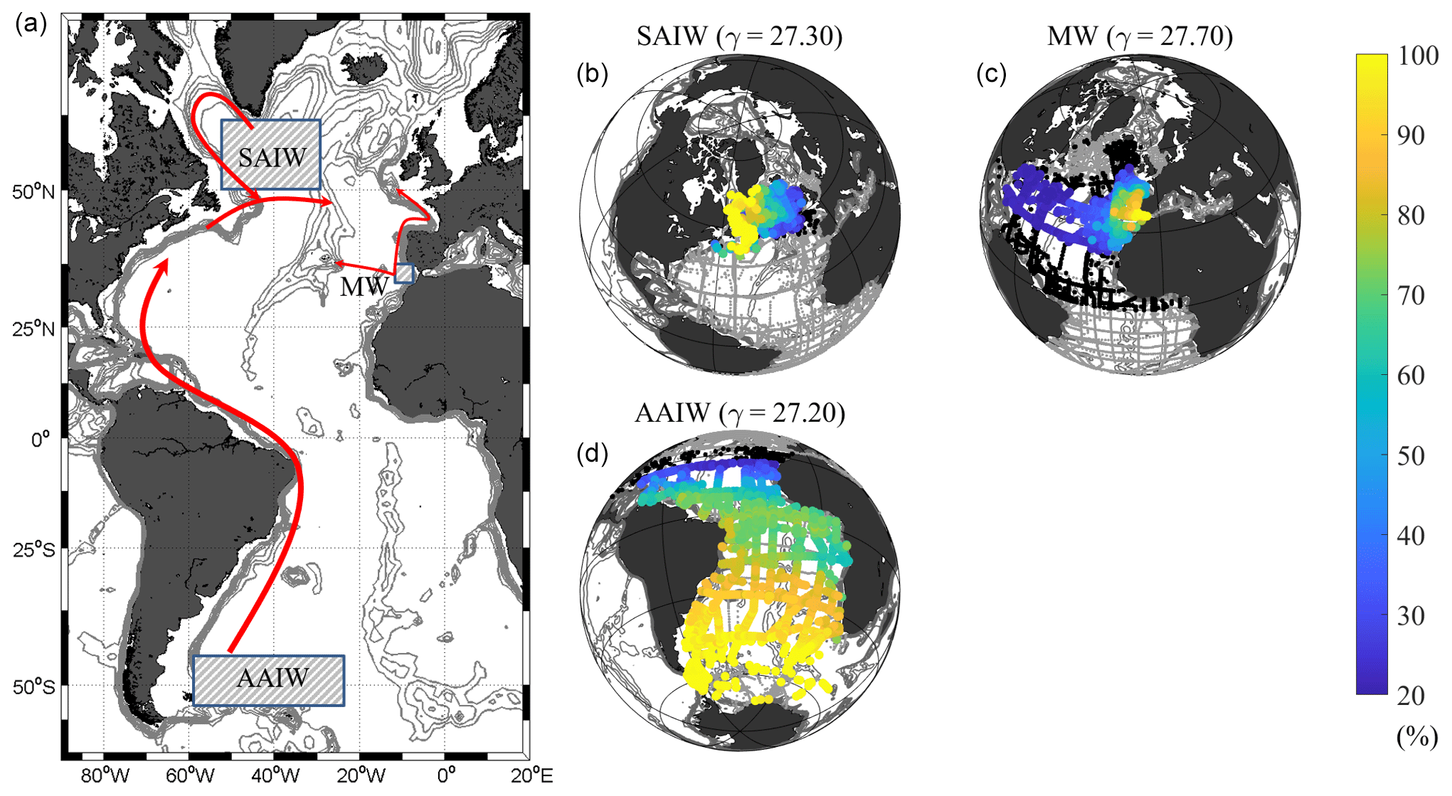
Figure 10 Currents (a) and water masses (b, c, d) in the intermediate layer. (a) The currents (arrows) and the formation areas (rectangular shadows) of water masses in the intermediate layer. (b, c, d) The coloured dots show fractions from 20 % to 100 % of water masses in each station around the core neutral densities (kg m⁻³). Stations with fractions less than 20 % are marked by black dots, while grey dots show all the GLODAPv2 stations.

In the Atlantic Ocean, two main intermediate water masses, Subarctic Intermediate Water (SAIW) and Antarctic Intermediate Water (AAIW), are formed in the surface of subpolar regions in Northern Hemisphere and Southern Hemisphere, respectively. In addition to AAIW and SAIW, MW is also considered as an intermediate water mass due to the similarity in density ranges, although the formation history is different (Fig. 10).

5.1 Antarctic Intermediate Water

AAIW is the main intermediate water in the South Atlantic Ocean. This water mass originates from the surface region north of the Antarctic Circumpolar Current (ACC) in all three sectors of the Southern Ocean, in particular in the area east of the Drake Passage in the Atlantic sector (McCartney, 1982; Alvarez et al., 2014), then subducts and spreads northward along the continental slope of South America (Piola and Gordon, 1989).

Based on the work by Stramma and England (1999) and Saenko and Weaver (2001), the region between 55 and 40^∘ S (east of the Drake Passage) at depths below 100 m is selected as the formation area of AAIW as well as the primary stage during the subduction and transformation phases (Fig. 5). Previous work is considered to distinguish AAIW from surrounding water masses, including SACW in the north and North Atlantic Deep Water (NADW) in the deep. Piola and Georgi (1982) and Talley (1996) define AAIW as potential densities (σ_θ) between 27.00–27.10 and 27.40 kg m⁻³, and Stramma and England (1999) define the boundary between AAIW and SACW at σ_θ=27.00 kg m⁻³ and the boundary between AAIW and NADW at σ₁ = 32.15 kg m⁻³. The following criteria are used as selection criteria to define AAIW: neutral density between 26.95 and 27.50 kg m⁻³ and depth between 100 and 300 m. In addition, high oxygen (> 260 µmol kg⁻¹) and low temperature (CT < 3.5 ^∘C) are used to distinguish AAIW from central waters (WSACW and ESACW), while the relative low silicate concentration (< 30 µmol kg⁻¹) of AAIW is an additional boundary to differentiate AAIW from Antarctic Bottom Water (AABW) (Table 2). The AAIW is distributed across most of the Atlantic Ocean up to ∼ 30^∘ N, and the water mass fraction shows a decreasing trend towards the north (Kirchner et al., 2009). AAIW is found at depths between 500 and 1200 m (Talley, 1996) with the two significant characteristic features of low salinity and high oxygen concentration (Fig. S4, Stramma and England, 1999).

5.2 Subarctic Intermediate Water

SAIW originates from the surface layer in the western boundary of the North Atlantic subpolar gyre, along the Labrador Current (Lazier and Wright, 1993; Pickart et al., 1997). This water mass subducts and spreads southeast in the region north of the North Atlantic Current (NAC), advects across the Mid-Atlantic Ridge and finally interacts with MW (Arhan, 1990; Arhan and King, 1995). The formation of SAIW is a mixture of two surface sources: water with high temperature and salinity carried by the NAC and cold and fresh water from the Labrador Current (Read, 2000; Garcia-Ibanez et al., 2015). In Garcia-Ibanez et al. (2015), there are two definitions of SAIW: SAIW₆, which is biased towards the warmer and saltier NAC, and SAIW₄, which is closer to the cooler and fresher Labrador Current. Here, only the combination of these two end-members is considered on the whole Atlantic Ocean scale (Fig. S5).

For defining the spatial boundaries, we followed Arhan (1990) and selected the region of 50–60^∘ N, 35–55^∘ W, i.e. the region along the Labrador Current and north of the NAC as the formation area of SAIW (Fig. 5). Within this area, neutral densities higher than 27.65 kg m⁻³ and CT higher than 4.5 ^∘C are selected to define SAIW following Read (2000). Samples in the depth range from the mixed layer depth (MLD) to 500 m are considered as the core layer of SAIW, which included the formation and subduction of SAIW (Table 2).

5.3 Mediterranean Water

The predecessor of MW is Mediterranean Overflow Water (MOW) flowing out through the Strait of Gibraltar, whose main component is modified Levantine Intermediate Water. This water mass is recognized by high salinity and temperature and intermediate neutral density in the Northeast Atlantic Ocean (Carracedo et al., 2016). After passing the Strait of Gibraltar, MOW mixes rapidly with the overlying ENACW and forms the MW, leading to a sharp decrease of salinity (Baringer and Price, 1997). In Gulf of Cádiz, the outflow of MW turns into two branches: one branch continues to the west, descending the continental slope, mixing with surrounding water masses in the intermediate depth and influence the water mass composition as far west as the MAR (Price et al., 1993). The other branch spreads northwards along the coast of Iberian Peninsula and along the European coast, and its influence can be observed as far north as the Norwegian Sea (Reid, 1978, 1979). The impact from MW is significant in almost the entire Northeast Atlantic in the intermediate layer (east of the MAR; Fig. S6), with high temperature and salinity but low nutrients compared to other water masses.

Here, we followed Baringer and Price (1997) and define the SWT of MW by the high salinity (SA between 36.5 and 37.00 g kg⁻¹; Table 2) samples in the formation area west of the Strait of Gibraltar (Fig. 5).

5.4 Atlantic distributions of intermediate waters

A schematic of the main currents in the intermediate layer (γ between 27.10 and 27.90 kg m⁻³) is shown in Fig. 10a.

SAIW is mainly formed north of 30^∘ N in the western basin by mixing of two main sources, the warmer and saltier NAC and the colder and fresher Labrador Current and characterized with relative low CT (< 4.5 ^∘C), SA (< 35.1 g kg⁻¹) and silicate (< 11 µmol kg⁻¹). SAIW and MW can be easily distinguished by the OMP analysis due to significantly different properties. The meridional distributions of three intermediate waters along the A16 section are shown in Fig. 11 (upper panel) together with the zonal distributions of SAIW and MOW along the A03 section. A “blob” of MW centred around 35^∘ N can be seen to separate AAIW from SAIW in the eastern North Atlantic. The fractions of SAIW in the western basin are definitely higher (Fig. 10b, c, d).

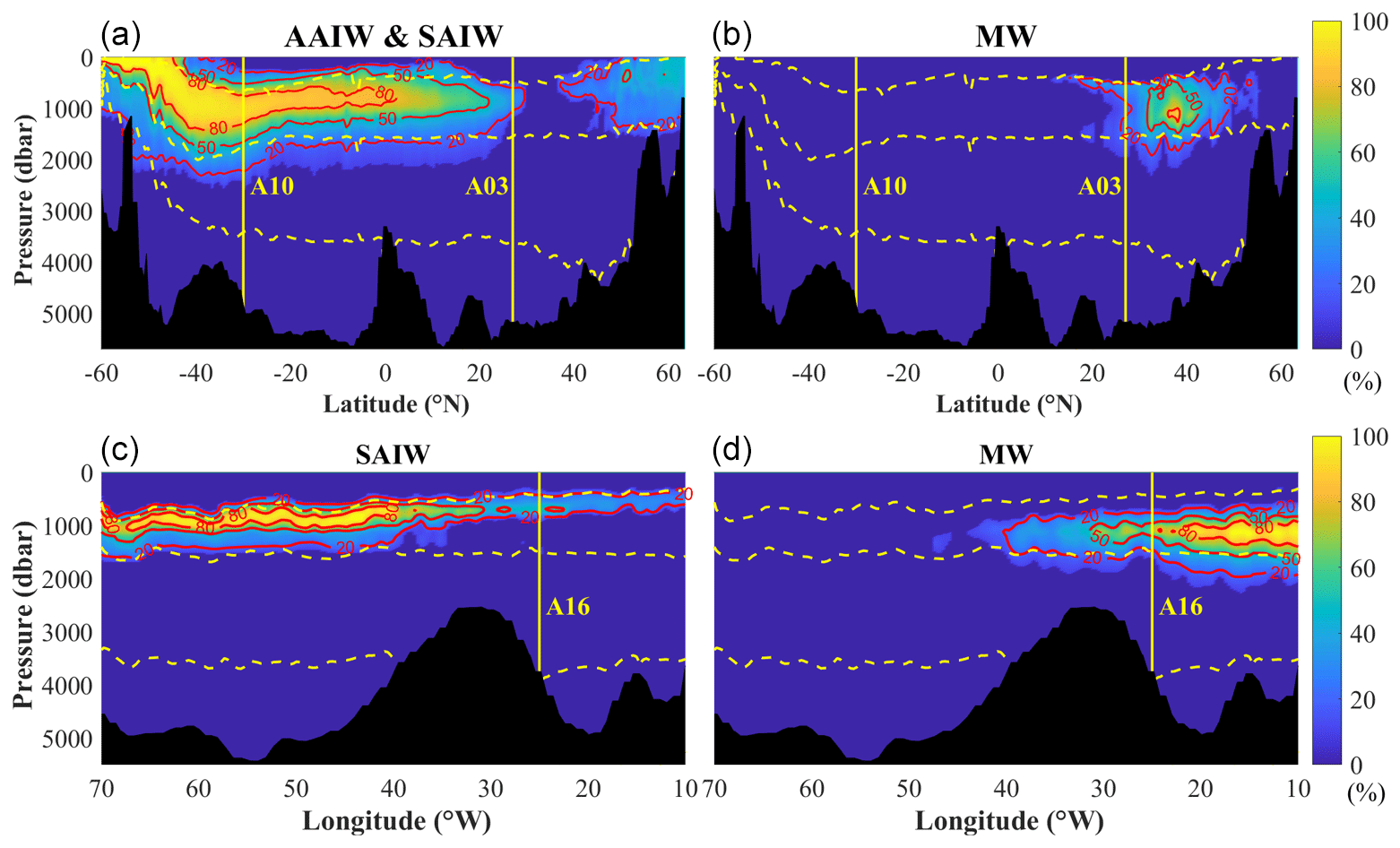
Figure 11 Distribution of water masses in the intermediate layer based on A16 (a, b) and A03 (c, d) sections. Contour lines show fractions of 20 %, 50 % and 80 %, yellow vertical lines show cross overs with other sections, and dashed yellow lines show the vertical boundaries of layers (neutral density at 27.10, 27.90 and 28.10 kg m⁻³).

MW enters the Atlantic from Strait of Gibraltar and spreads in two branches to the north and the west. MW is mainly formed close to its entry point to the Atlantic, near the Gulf of Cádiz, with low fractions in the western North Atlantic. The distribution of MW can be seen as roughly following the two intermediate pathways following two branches (Fig. 10a): one spreads to the north into the west European basin until ∼ 50^∘ N, while the other branch spreads in a westward direction past the MAR (Fig. 11), mainly at latitudes between 30 and 40^∘ N. The density of MW is higher than SAIW, and the distributions of the two water masses are complementary in the North Atlantic (Fig. 10b, c, d).

AAIW has a southern origin and is found at slightly lighter densities (core neutral density ∼ 27.20 kg m⁻³, Fig. 10b, c, d) compared to SAIW and MW. AAIW is formed in the region south of 40^∘ S, where it sinks and spreads to the north at depth between ∼ 1000 and 2000 m with neutral densities between 27.10 and 27.90 kg m⁻³. AAIW is the dominant intermediate water in the South Atlantic, and it is clear that AAIW represents a reduction of fractions during the pathway to the north with only a diluted part to be found at the Equator and 30^∘ N (Figs. 10 and 11).

6 The deep and overflow layer

The deep and overflow waters are found roughly between 2000 to 4000 m with neutral densities between 27.90 and 28.10 kg m⁻³. These water masses play an indispensable role in the Atlantic Meridional Overturning Circulation (AMOC). The source region of these waters is confined to the North Atlantic with their formation region either south of the Greenland–Scotland Ridge or in the Labrador Sea (Figs. 5 and 12). The DSOW and the Iceland–Scotland Overflow Water (ISOW) originate from Arctic Ocean and the Nordic Seas and enter the North Atlantic through either the Denmark Strait of the Faroe Bank Channel (Fig. 12a). In the North Atlantic, these two water masses descend, mainly following the topography meet and mix in the Irminger Basin (Stramma et al., 2004; Tanhua et al., 2005) and form the bulk of the lower North Atlantic Deep Water (lNADW) (Read, 2000; Rhein et al., 2011). Labrador Sea Water (LSW) is formed through winter deep convection in the Labrador and Irminger seas and makes up the bulk of the upper North Atlantic Deep Water (uNADW). Due to intense mixing processes the LSW, DSOW and ISOW are defined as the water masses in north of 40^∘ N, whereas south of this latitude the presence of the two variations of NADW are considered (Fig. 12).

South of 40^∘ N, both variations of NADW spread south mainly with the Deep Western Boundary Current (DWBC; Fig. 12a) (Dengler et al., 2004) through the Atlantic until ∼ 50^∘ S, where they meet the ACC. During the southward transport, NADW also spreads significantly in the zonal direction (Lozier, 2012), so that the distribution of NADW covers mostly the whole Atlantic basin in the deep and overflow layer (Fig. 12, right panel). The southward flow of NADW is also an indispensable component of the AMOC (Broecker and Denton, 1989; Elliot et al., 2002; Lynch-Stieglitz et al., 2007).

6.1 Labrador Sea Water

As an important water mass that contributes to the formation of North Atlantic Deep Water (NADW), LSW is predominant in mid-depth (between 1000 and 2500 m depth) in the Labrador Sea region (Elliot et al., 2002). This water mass was firstly noted by Wüst and Defant (1936) due to its salinity minimum and later defined and named by Smith et al. (1937). The LSW is formed by deep convection during the winter and is typically found at depth with σ_θ= ∼ 27.77 kg m⁻³ (Clarke and Gascard, 1983). Since then, the characteristic has been identified as a contribution to the driving mechanism of northward heat transport in the AMOC (Rhein et al., 2011). The LSW is characterized by relative low salinity (lower than 34.9) and high oxygen concentration (∼ 290 µmol kg⁻¹) (Talley and Mccartney, 1982). Another important criterion of LSW is the potential density (σ_θ), which ranges from 27.68 to 27.88 kg m⁻³ (Clarke and Gascard, 1983; Gascard and Clarke, 1983; Stramma et al., 2004; Kieke et al., 2006). On a large spatial scale, LSW can be considered as one water mass (Dickson and Brown, 1994); however, significant differences of different “vintages” of LSW exist (Stramma et al., 2004; Kieke et al., 2006). In some references, this water mass is also broadly divided into upper Labrador Sea Water (uLSW) and classic Labrador Sea Water (cLSW), with the boundary between them at potential density of 27.74 kg m⁻³ (Smethie and Fine, 2001; Kieke et al., 2006, 2007). The LSW is considered as the main origin of the upper NADW (Talley and Mccartney, 1982; Elliot et al., 2002).

On the basis of the above work, the formation area of LSW is selected to include the Labrador Sea region between the Labrador Peninsula and Greenland and parts of the Irminger Basin (Fig. 5). Neutral density (γ) between 27.70 to 28.10 kg m⁻³ as well as CT < 4 ^∘C are used to define SWT of LSW (Table 2) by considering Clarke and Gascard (1983) and Stramma and England (1999) with the depth range of 500–2000 m (Elliot et al., 2002). Trademark characteristics of LSW are relative low salinity and high oxygen. The relatively large spread in properties is indicative of the different “vintages” of LSW, in particular the bi-modal distribution of density, and partly of oxygen (Fig. S7).

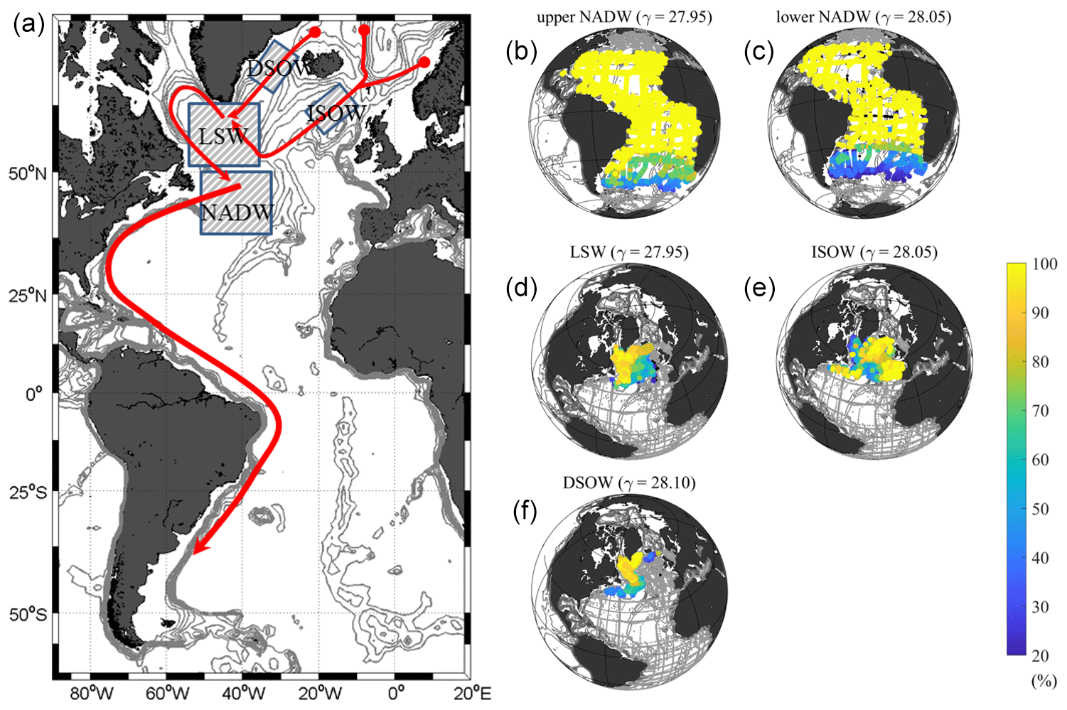
Figure 12 Currents (a) and water masses (b, c, d, e, f) in the deep and overflow layer. (a) The currents (arrows) and the formation areas (rectangular shadows) of water masses in the deep and overflow layer. (b, c, d, e, f) The coloured dots show fractions (from 20 % to 100 %) of water masses in each station around core neutral density (kg m⁻³). Stations with fractions less than 20 % are marked by black dots, while grey dots show all the GLODAPv2 stations.

6.2 Iceland–Scotland Overflow Water

ISOW flows close to the bottom from the Iceland Sea to the North Atlantic in the region east of Iceland, mainly through the Faroe Bank Channel (Swift, 1984; Lacan et al., 2004; Zou et al., 2020). ISOW turns into two main branches before passing the Charlie–Gibbs Fracture Zone (CGFZ), with the first one flowing through the Mid-Atlantic Ridge, into the Irminger Basin, where it meets and mixes with DSOW (Fig. 12). The other branch is transported southward and mixes with Northeast Atlantic Bottom Water (NEABW) (Garcia-Ibanez et al., 2015). ISOW is characterized by high nutrient and low oxygen concentration, and its pathway closely follows the Mid-Atlantic Ridge in the Iceland Basin. The following criteria (conservative temperature between 2.2 and 3.3 ^∘C and absolute salinity higher than 34.95 g kg⁻¹) are used to define the SWT of ISOW, and neutral density higher than 28.00 kg m⁻³ is added order to distinguish ISOW from LSW in the region west of MAR (Table 2 and Fig. S8).

6.3 Denmark Strait Overflow Water

A number of water masses from the Arctic Ocean and the Nordic Seas flow through the Denmark Strait west of Iceland. At the sill of the Denmark Strait and during the descent into the Irminger Sea, these water masses undergo intense mixing. This overflow water mass is considered the coldest and densest component of the sea water in the Northwest Atlantic Ocean and constitutes a significant part of the southward-flowing NADW (Swift, 1980). Samples from the Irminger Sea (Fig. 5) with neutral density higher than 28.15 kg m⁻³ (Table 2 and Fig. S9) are used for the definition of DSOW (Rudels et al., 2002; Tanhua et al., 2005).

6.4 Upper North Atlantic Deep Water

uNADW is mainly formed by mixing of ISOW and LSW and considered as a distinct water mass south of the Labrador Sea, as this region is identified as the redefining area of upper and lower NADW (Dickson and Brown, 1994). The region between latitude 40 and 50^∘ N, west of the MAR, is selected as the redefining area of NADW (Fig. 5), and the criteria of neutral density between 27.85 and 28.05 kg m⁻³ and CT < 4.0 ^∘C within the depth range from 1200 to 2000 m (Table 2 and Fig. S10) are used to define the SWT of uNADW (Stramma et al., 2004). As a mixture of LSW and ISOW, uNADW obviously inherits many properties from LSW but is also significantly influenced by ISOW. The relatively high temperature (∼ 3.3 ^∘C) is a significant feature of the uNADW together with relatively low oxygen (∼ 280 µmol kg⁻¹) and high nutrient concentrations, which is a universal symbol of deep water (Table 4 and Fig. S10).

6.5 Lower North Atlantic Deep Water

The same geographic region is selected as the formation area of lNADW (Fig. 5). In this region, ISOW and DSOW, influenced by LSW, mix with each other and form the lower portion of NADW (Stramma et al., 2004). Water samples between depths of 2000 and 3000 m with CT higher than ∼ 2.5 ^∘C and neutral densities between 27.95 and 28.10 kg m⁻³ are selected to define the SWT of lNADW (Table 2 and Fig. S11).

6.6 Atlantic distributions of deep and overflow waters

The water masses that dominate the neutral density interval of 27.90–28.10 kg m⁻³ in the Atlantic Ocean north of 40^∘ N are LSW, ISOW and DSOW. In the region south of 40^∘ N, the upper and lower NADW, considered as products of these three original overflow water masses, dominate the deep and overflow layer (Fig. 12).

LSW is commonly characterized as two variations, “upper” and “classic”, although in this study we consider this as one water mass in the discussion above. Our analysis indicates that the LSW dominates the Northwest Atlantic Ocean in the characteristic density range. In Fig. 12, we choose to display γ=27.95, which corresponds to the main property of the LSW (Kieke et al., 2006, 2007). The LSW spreads eastward and southward in the North Atlantic Ocean but is less dominant in the area west of the Iberian Peninsula where the presence of MW from the Gulf of Cádiz tends to dominate that density level. Note that although the LSW is slightly denser than the MW, their density ranges do overlap (Figs. 12 and 13).

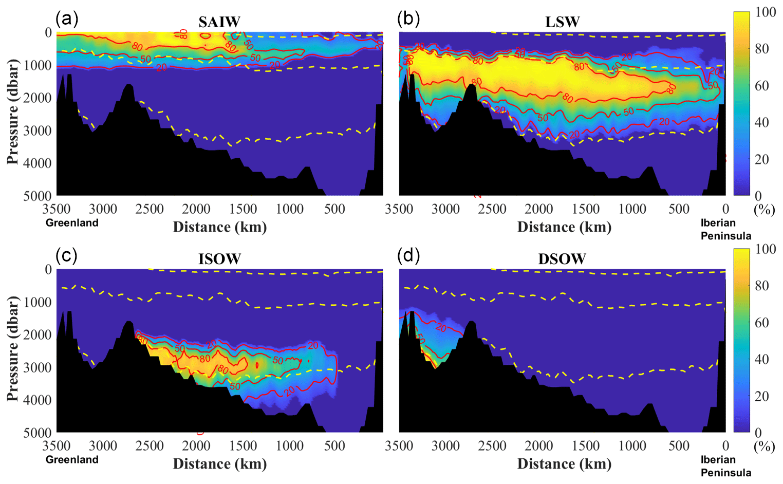
Figure 13 Distribution of SAIW (a), LSW (b), ISOW (c) and DSOW (d) based on the A25 section. Contour lines show fractions of 20 %, 50 % and 80 %, and dashed yellow lines show the vertical boundaries of layers (neutral density at 27.10, 27.90 and 28.10 kg m⁻³).

ISOW is mainly found in the Northeast Atlantic north of 40^∘ N between Iceland and the Iberian Peninsula with the core at $\mathit{\gamma }=\sim$ 28.05 kg m⁻³. The ISOW is also found west of the Reykjanes Ridge, in the Irminger and Labrador seas between the DSOW and LSW (Figs. 12 and 13).

DSOW is mainly found in the Irminger and Labrador seas, as the densest layer close to the bottom (Fig. 11). Our analysis indicates a weak contribution of DSOW also east of the MAR. South of the Grand Banks, DSOW is already significantly diluted and only low-to-moderate fractions are found (Figs. 12 and 13).

After passing 40^∘ N, the upper and lower NADW are considered as independent water masses and dominate the most of the Atlantic Ocean in this density layer. The map in Fig. 12 shows that upper NADW covers the most area, while lower NADW is found mainly found in the west region near the DWBC, especially in the South Atlantic. In the vertical view based on sections (Fig. 14), the southward transport of both upper and lower NADW can be seen until ∼ 50^∘ S, where they meet AABW in the ACC region.

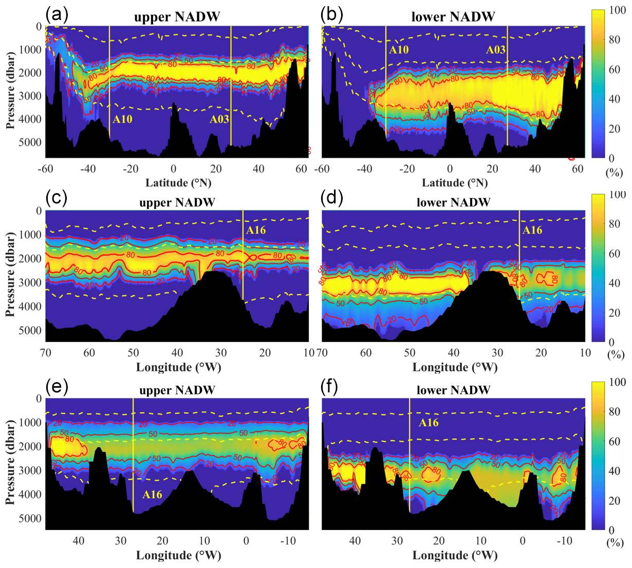
Figure 14 Distribution of upper and lower NADW based on the A16 (a, b), A03 (c, d) and A10 (e, f) sections. Contour lines show fractions of 20 %, 50 % and 80 %, yellow vertical lines show cross overs with other sections, and the dashed yellow lines show the vertical boundaries of layers (neutral density at 27.10, 27.90 and 28.10 kg m⁻³).

7 The bottom layer and the southern water masses

The bottom waters are defined as the densest water masses that occupy the lowest layers of the water column, typically below 4000 m depth and with neutral densities higher than 28.10 kg m⁻³. These water masses have an origin in the Southern Ocean (Fig. 15a) and are characterized by their high silicate concentrations. The AABW is the main water mass in the bottom layer (Fig. 15a). This water mass is formed in the Weddell Sea region, south of ACC, through mixing of Circumpolar Deep Water (CDW) and Weddell Sea Bottom Water (WSBW) (van Heuven et al., 2011). After the formation, AABW spreads to the north across the Equator and further northwards until ∼ 40^∘ N (Fig. 16), where a new SWT is redefined as NEABW due to the drastic change in properties (sharp decrease in silicate concentration). As the two main sources of AABW (CDW and WSBW) are confined to the Southern Ocean (Fig. 15), they are referred to as the southern water masses and discussed in this section together with bottom waters.

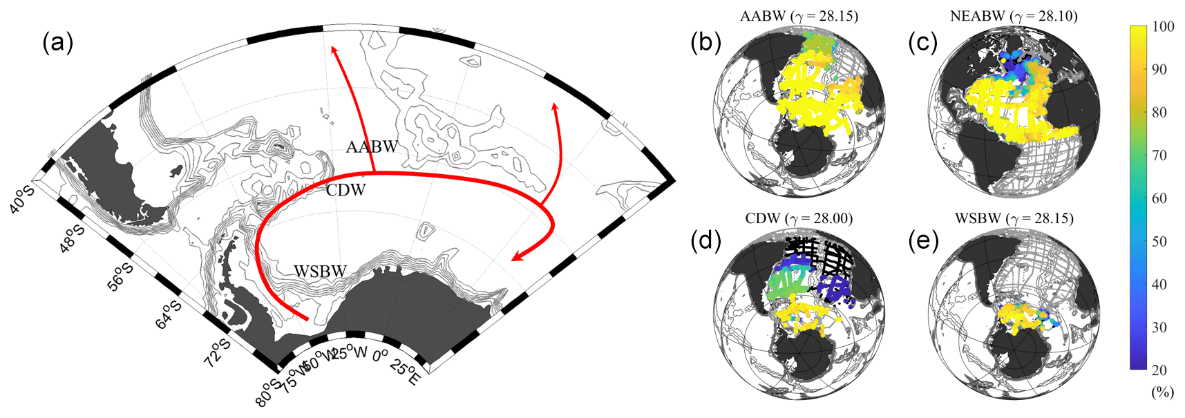
Figure 15 Currents (a) and water masses (b, c, d, e) in the bottom layer (AABW and NEABW) and the southern area (CDW and WSBW). (a) The arrows show the main currents in the southern area. (b, c, d, e) The coloured dots show fractions (from 20 % to 100 %) of water masses in each station around core neutral density (kg m⁻³). Stations with fractions less than 20 % are marked by black dots, while grey dots show all the GLODAPv2 stations.

7.1 Antarctic Bottom Water

AABW is the symbolic bottom water of the whole Atlantic Ocean. As one of the important components in the AMOC, AABW spreads northward below 4000 m depth, mainly west of the MAR (Fig. 15a), and plays a significant role in the thermohaline circulation (Rhein et al., 1998; Andrié et al., 2003). The origin of AABW in Atlantic section can be traced back to the Weddell Sea as a product of mixing of WSBW and CDW (Foldvik and Gammelsrod, 1988; Alvarez et al., 2014).

Figure 16 Distribution of AABW and NEABW based on A16 (a, b), A10 (c) and A03 (d) sections. Contour lines show fractions of 20 %, 50 % and 80 %, yellow vertical lines show cross overs with other sections, and dashed yellow lines show the boundaries of vertical water columns layers (neutral density at 27.10, 27.90 and 28.10 kg m⁻³).

The definition of AABW is all water samples formed south of the ACC, i.e. south of 63^∘ S in the Weddell Sea (Fig. 5), with neutral density (γ) larger than 28.27 kg m⁻³ (Weiss et al., 1979; Orsi et al., 1999). As an additional constraint, AABW is defined as water samples with silicate higher than 120 µmol kg⁻¹ to distinguish it from other water masses in this region, as high silicate is a trademark property of AABW (Table 2).

The formation process of AABW is a mixture of another two original water masses, CDW and WSBW, which are referred to as southern water masses, in the Weddell Sea region, consistent with Orsi et al. (1999) and van Heuven et al. (2011). The CDW, with relatively warm temperature (CT > 0.4 ^∘C), is advected with the ACC from the north, while the extremely cold shelf water (CT < −0.7 ^∘C) comes as WSBW from the south (Fig. 17). AABW is found from 1000 to 5500 m depth (Figs. 16 and 17) with low temperature (CT < 0 ^∘C), salinity (SA < 34.68) but high nutrient, especially silicate, concentrations (Fig. S12).

Figure 17 Distribution of southern water masses (CDW, AABW and WSBW) based on SR04 sections. Panels (a), (c) and (e) show the west (zonal) part, and (b), (d) and (f) show the east (meridional) part of the section. The contour lines show fractions of 20 %, 50 % and 80 %.

7.2 Northeast Atlantic Bottom Water

NEABW, also called lower Northeast Atlantic Deep Water (lNEADW; Garcia-Ibanez et al., 2015), is mainly found below 4000 m depth in the eastern basin of the North Atlantic (Fig. 5). This water mass is an extension of AABW during the way to the north, since the properties of AABW change significantly on the slow transport north. A new SWT is redefined for this water mass north of the Equator, similar to the redefinition of NADW south of the Labrador Sea.

The region east of the MAR and between the Equator and 30^∘ N, i.e. before NEABW enters the Iberian Basin, is selected as the redefining area of NEABW. The criteria of depth deeper than 4000 m and CT above 1.8 ^∘C are also used (Table 2). In the CT–SA diagram in Fig. 3, a similar T–S distribution between NEABW and AABW can be seen but with higher CT and SA of ∼ 1.95 ^∘C and ∼ 35.060 g kg⁻¹. Most NEABW samples have a neutral density higher than 28.10 kg m⁻³, and NEABW is characterized by low CT and SA but high silicate concentration (Fig. S13). This further suggests that NEABW originates from AABW, although most properties have been changed significantly from the origin in the South Atlantic.

7.3 Circumpolar Deep Water

CDW, which has significance to the thermohaline circulation during the wind-driven upwelling in the Southern Ocean (Morrison et al., 2015), is the lighter of the two water masses that contribute to AABW formation. The production of this water mass can be tracked to the southward flow of NADW and the large-scale mixing in the ACC region (van Heuven et al., 2011). At about 50^∘ S, NADW is deflected upward by AABW before reaching the ACC (Fig. 14a, b); this part of NADW spreads further southward into the ACC region, where it connects with other water masses, including AAIW above and AABW below. After passing the ACC region, CDW splits into two branches at ∼ 60^∘ S. The upper branch is upwelled and partly joins the AAIW, while the rest spreads towards the coastal region, mixes with the cold fresh shelf water, sinks to the bottom and finally forms WSBW, which is another contribution to AABW (Marshall and Speer, 2012; Abernathey et al., 2016). The lower branch sinks and mixes with WSBW below and contributes to the formation of AABW.

In this study, the SWTs of CDW are defined by considering the lower branch, and the region between 55 and 65^∘ S is selected as the formation area (Fig. 5). To define SWT of CDW (lower branch), water samples are selected from the depth between 200 and 1000 m in this region, and additional constraints are an SA higher than 34.82 g kg⁻¹ and CT between −0.5 and 1.0 ^∘C (Table 2). Similar to other bottom/southern SWTs, CDW is also defined by high nutrient (silicate, phosphate and nitrate) and low oxygen concentrations (Fig. S14).

7.4 Weddell Sea Bottom Water

WSBW is the densest water mass in the bottom layer. As mentioned in the above section, part of CDW from the upper branch cools down rapidly by mixing with extremely cold shelf water and sinks down to the bottom along the continental slop (Gordon, 2001). WSBW is formed in the Weddell Sea basin below the depth of 3000 m before it meets and mixes with CDW. The low temperature of WSBW compared to CDW (CT of ∼ −0.8 ^∘C) is a characteristic property (Fig. S15; van Heuven et al., 2011).

Water samples in the latitudinal boundaries of 55–65^∘ S in the Weddell Sea (Fig. 5), with pressures larger than 3000 m, CT lower than −0.7 ^∘C and silicate higher than 105 µmol kg⁻¹, are selected to define the SWT of WSBW (Table 2), following Gordon (2001) and van Heuven et al. (2011).

7.5 Atlantic distribution of the bottom waters and southern water masses

AABW and NEABW dominate the bottom layer (γ> 28.10 kg m⁻³). From the horizontal distribution (Fig. 15), it can be seen that AABW and NEABW cover the lowest area of the South and North Atlantic, respectively. In fact, both water masses have the same origin but are distinguished by redefining a new SWT due to the sharp reduction of silicate after passing the Equator (Fig. 16). AABW is formed in the Weddell Sea region south of the ACC. After leaving the formation area, AABW sinks to the bottom due to the high density during the way north. After passing the ACC, AABW suffers from water exchange with NADW between 50^∘ S and the Equator (van Heuven et al., 2011). Similar to AABW, NEABW also mainly contacts with lower NADW and its origin (ISOW) in the North Atlantic (Garcia-Ibanez et al., 2015).

In the Weddell Sea region, distributions of water masses mainly reflect the formation process of AABW as displayed based on SR04 sections (Fig. 17). In the zonal section, AABW can be seen as the mixture of CDW and WSBW, where the core of CDW is distributed in the upper 1000 m, and WSBW originates from the surface and sinks along the continental slope into the bottom below 4000 m. Both original water masses meet each other at depths between ∼ 2000 and 4000 m, where AABW is formed, with main core locates at ∼ 3000 m. The meridional section shows the northward outflow of AABW into the Atlantic Ocean. AABW is located between 2000 and 4000 m as a product of CDW and WSBW. After leaving Weddell Sea region, AABW is considered as an independent water mass and spreads further northward as the only bottom water mass until the Equator.

8 Conclusions and discussion

The characteristics of the main water masses in their formation areas are defined in a six-dimensional hydrochemical space in the Atlantic Ocean. The values of properties for these water masses form the fundamental basis to investigate their transport, distribution and mixing and are referred to as SWTs. Table 4 and Fig. 3 provide an overview SWTs of all 16 Atlantic Ocean main water masses considered in this study. The distributions of water masses are estimated by using OMP analysis based on the GLODAPv2 data product and preliminarily divided into four vertical layers based on neutral densities.

The upper layer, which covers the most shallow layer (typically down to about 500 m depth) of the ocean below the mixed layer (the mixed layer is not considered in this analysis), is occupied by central waters. The intermediate layer is situated between the upper layer and the deep and overflow layer at roughly 1000 to 2000 m depth. Of the three water masses in this layer, AAIW and SAIW are both characterized by relative low salinity and temperature, while MW has high SA and CT. SAIW and MW show a northwest–southeast distribution in the North Atlantic, while AAIW dominates the intermediate layer of the region south of 30^∘ N. In the deep and overflow layer between roughly 2000 and 4000 m, NADW, which contains upper and lower portions, is recognized as the dominant water mass with a relative complex origin from LSW, ISOW and DSOW. The bottom layer is occupied by AABW, with a southern origin formed by CDW and WSBW. After passing the Equator, this water mass is redefined as NEABW due to the changes in properties (silicate).

Besides the 16 main Atlantic Ocean water masses, additional water masses still exist and can be found in the Atlantic that cannot be explained by the mixing of any above listed original water masses. This tends to happen close to the coast by local oceanographic events; such water masses are not listed and considered as main water masses in this study, and no additional SWTs are defined. For instance, in the coastal region of the southern Benguela upwelling system (30–34^∘ S, 15–20^∘ E), water samples are found with low temperature and oxygen (∼ 8 ^∘C and ∼ 150 µmol kg⁻¹, respectively). This cannot be explained by the mixing of ESACW and WSACW, which are the only two possible water masses in this region and depth, because the CT and oxygen of both water masses are higher than these values. One possible explanation is that low-oxygen water is transported by upwelling (Flynn et al., 2020).

The here-presented characteristics (property values and the standard deviations) of Atlantic Ocean water masses and their distributions are intended to guide water mass analysis of hydrographic data and expect to provide a basis for further biogeochemical research.