the Creative Commons Attribution 4.0 License.
the Creative Commons Attribution 4.0 License.
 | 28 Jan 2021
Spiciness theory revisited, with new views on neutral density, orthogonality, and passiveness
Rémi Tailleux
This paper clarifies the theoretical basis for constructing spiciness variables optimal for characterising ocean water masses. Three essential ingredients are identified: (1) a material density variable γ that is as neutral as feasible, (2) a material state function ξ independent of γ but otherwise arbitrary, and (3) an empirically determined reference function ξr(γ) of γ representing the imagined behaviour of ξ in a notional spiceless ocean. Ingredient (1) is required because contrary to what is often assumed, it is not the properties imposed on ξ (such as orthogonality) that determine its dynamical inertness but the degree of neutrality of γ. The first key result is that it is the anomaly , rather than ξ, that is the variable most suited for characterising ocean water masses, as originally proposed by McDougall and Giles (1987). The second key result is that oceanic sections of normalised ξ′ appear to be relatively insensitive to the choice of ξ, as first suggested by Jackett and McDougall (1985), based on the comparison of very different choices of ξ. It is also argued that the orthogonality of ∇ξ′ to ∇γ in physical space is more germane to spiciness theory than orthogonality in thermohaline space, although how to use it to constrain the choices of ξ and ξr(γ) remains to be fully elucidated. The results are important for they unify the various ways in which spiciness has been defined and used in the literature. They also provide a rigorous theoretical basis justifying the pursuit of a globally defined material density variable maximising neutrality. To illustrate the latter point, this paper proposes a new implementation of the author's recently developed thermodynamic neutral density and explains how to adapt existing definitions of spiciness and spicity to work with it.
- Article
(11571 KB) - Full-text XML
- BibTeX
- EndNote


As is well known, three independent variables are needed to fully characterise the thermodynamic state of a fluid parcel in the standard approximation of seawater as a binary fluid. The standard description usually relies on the use of a temperature variable (such as potential temperature θ, in situ temperature T, or Conservative Temperature Θ), a salinity variable (such as reference composition salinity S or Absolute Salinity SA), and pressure p. In contrast, theoretical descriptions of oceanic motions only require the use of two “active” variables, namely in situ density ρ and pressure. The implication is that S and θ can be regarded as being made of an active part contributing to density and a passive part associated with density-compensated variations in θ and S – usually termed “spiciness” anomalies – which behaves as a passive tracer. Physically, such an idea is empirically supported by numerical simulation results showing that the turbulence spectra of density-compensated thermohaline variance is generally significantly different from that contributing to the density (Smith and Ferrari, 2009).
Although behaving predominantly as passive tracers, density-compensated anomalies may occasionally “activate” and couple with density and ocean dynamics. This may happen, for instance, when isopycnal mixing of θ and S leads to cabbeling and densification, which may create available potential energy (Butler et al., 2013); when density-compensated temperature anomalies propagate over long distances to de-compensate upon reaching the ocean surface, thus modulating air–sea interactions (Lazar et al., 2001); when density-compensated salinity anomalies propagate from the equatorial regions to the regions of deepwater formation, thus possibly modulating the strength of the thermohaline circulation (Laurian et al., 2006, 2009); and/or when isopycnal stirring of density-compensated anomalies releases available potential energy associated with thermobaric instability (Ingersoll, 2005; Tailleux, 2016a). For these reasons, the mechanisms responsible for the formation, propagation, and decay of spiciness anomalies have received much attention, with a key research aim being to understand their impacts on the climate system; e.g. Schneider (2000), Yeager and Large (2004), Luo et al. (2005), Tailleux et al. (2005), and Zika et al. (2020).
From a dynamical viewpoint, in situ density ρ is the most relevant density variable for defining density-compensated anomalies, but its strong pressure dependence makes the associated isopycnal surfaces strongly time-dependent and therefore impractical to use. This is why in practice oceanographers prefer to work with isopycnal surfaces defined by means of a purely material density-like variable unaffected by pressure variations. Since density-compensated anomalies are truly passive only if defined in terms of in situ density, γ needs to be able to mimic the dynamical properties of in situ density as much as feasible. As discussed by Eden and Willebrand (1999), this amounts to imposing that γ be constructed to be as neutral as feasible. Because of the thermobaric non-linearity of the equation of state, it is well known that exact neutrality cannot be achieved by any material variable. As a result, investigators have resorted to using either neutral surfaces (McDougall and Giles, 1987) or potential density referenced to a pressure close to the range of pressures of interest (Jackett and McDougall, 1985; Huang, 2011; McDougall and Krzysik, 2015; Huang et al., 2018). In this paper, I propose instead using a new implementation of the Tailleux (2016b) thermodynamic neutral density variable γT, which is currently the most neutral material density-like variable available. The resulting new variable is referred to as in the following, and details of its construction and implementation are given in Sect. 2.
Once a choice for γ has been made, a second material variable is required to fully characterise the thermodynamic properties of a fluid parcel. From a mathematical viewpoint, the only real constraint on ξ is that the transformation defines a continuously differentiable one-to-one mapping (that is, an isomorphism) so that (S,θ) properties can be recovered from the knowledge of (γ,ξ). For this, it is sufficient that the Jacobian differs from zero everywhere in (S,θ) space where invertibility is required. Historically, however, spiciness theory appears to have been developed on the predicate that for ξ to be dynamically inert, it should be constructed to be “orthogonal” to γ in (S,θ) space, as originally put forward by Veronis (1972) (whose variable is denoted by τν in the following). This notion was argued to be incorrect by Jackett and McDougall (1985), however, who pointed out the following: “[…] the variations of any variable, when measured along isopycnal surfaces, are dynamically passive and so the perpendicular property does not, of itself, contribute to the dynamic inertness of τν”, to which they added the following. “Secondly, it is readily apparent that the perpendicular property itself has no inherent physical meaning since a simple rescaling of either the potential temperature θ or the salinity axis S destroys the perpendicular property”. The Jackett and McDougall (1985) remarks are important for at least two reasons: (1) first, for suggesting that it is really the isopycnal anomaly defined relative to some reference function of density ξr(γ) that is dynamically passive and therefore the quantity truly measuring spiciness. This was further supported by McDougall and Giles (1987) subsequently arguing that it is such an anomaly that represents the most appropriate approach for characterising water mass intrusions. Note here that if one defines reference salinity and temperature profiles Sr(γ) and θr(γ) such that , using a Taylor series expansion shows that and are γ-compensated at leading order, i.e. they satisfy , and hence approximately passive. (2) The second reason is for establishing that the imposition of any form of orthogonality between ξ and γ is even less meaningful than previously realised, since even if ξ is constructed to be orthogonal to γ in some sense, this orthogonality is lost by the anomaly .
If one accepts that it is the spiciness anomaly rather than the spiciness as a state function (ξ) that is the most appropriate measure of water mass contrasts, as argued by Jackett and McDougall (1985) and McDougall and Giles (1987), the central questions that the theory of spiciness needs to address become the following.
-
Are there any special benefits associated with one particular choice of spiciness as a state function (ξ) over another, and if so, what are the relevant physical arguments that should be invoked to establish the superiority of any given particular choice of ξ?
-
How should γ and the reference function ξr(γ) be constructed and justified?
-
While any ξ independent of γ can be used to meaningfully compare the spiciness of two different water samples lying on the same isopycnal surface γ=constant, it is generally assumed that it is not possible to meaningfully compare the spiciness of two water samples belonging to two different isopycnal surfaces γ1 and γ2 (Timmermans and Jayne, 2016). Is this belief justified? Is the transformation of ξ into an anomaly ξ′ sufficient to address the issue?
Regarding the first question, Jackett and McDougall (1985) have developed geometrical arguments in support of a variable τjmd satisfying along potential density surfaces that they argue make it superior to other choices. These arguments do not seem to be decisive, however, since τjmd does not satisfy the above-mentioned invertibility constraint where the thermal expansion α vanishes. At such points, temperature becomes approximately passive and therefore the most natural definition of spiciness as pointed out by Stipa (2002). At such points, however, the Jackett and McDougall (1985) variable, like the Flament (2002) variable, behaves like salinity, causing the Jacobian of the transformation to vanish, which seems unphysical. The ability of different kinds of anomalies, namely , , and S′, to characterise water mass contrasts and intrusions is discussed in the second part of the Jackett and McDougall (1985) paper. Interestingly, they find that even though the spiciness as state functions τν, τjmd, and S behave quite differently from each other in (S,θ) space, their anomalies exhibit in contrast only small differences, at least when estimated for individual soundings. In this paper, I show that this property actually appears to be satisfied much more broadly, as illustrated in Fig. 12 and further discussed in the text.
Orthogonality in (S,θ) space – despite its usefulness or necessity remaining a source of confusion and controversy – has nevertheless been central to the development of spiciness theory. Recently, Huang et al. (2018) attempted to rehabilitate the Veronis (1972) form of orthogonality by arguing that without imposing it, it is otherwise hard to define a distance in (S,θ) space. This argument is unconvincing, however, because the concept of distance in mathematics does not require orthogonality; it only requires the introduction of a positive definite metric d(x,y), i.e. one satisfying the following: (1) for all x and y; (2) is equivalent to x=y; (3) ; and (4) , the so-called triangle inequality. As a result, there is an infinite number of ways to define distance in (S,θ) space. For instance, , where α0 and β0 are some constant reference values of α and β, is an acceptable definition of distance. Likewise, any two non-trivial and independent material functions γ(S,θ) and ξ(S,θ) could also be used to define , where K0 is a constant to express γ and ξ in the same system of units if needed, while γA is shorthand for γ(SA,θA), with similar definitions for γB, ξA, and ξB. In regards to the 45∘ orthogonality proposed by Jackett and McDougall (1997) and Flament (2002), while it is true that it is unaffected by a re-scaling of the S and θ axes plaguing the Veronis (1972) form of orthogonality, it is destroyed by the subtraction of any function of potential density while also causing the above-mentioned loss of invertibility where α vanishes. In any case, it is unclear why Jackett and McDougall (1997) sought to impose the 45∘ orthogonality to τjmd, since it is a priori not necessary to satisfy the above-mentioned constraint on isopycnal surfaces (in the sense that if one particular τjmd solves the problem, any will also solve it).
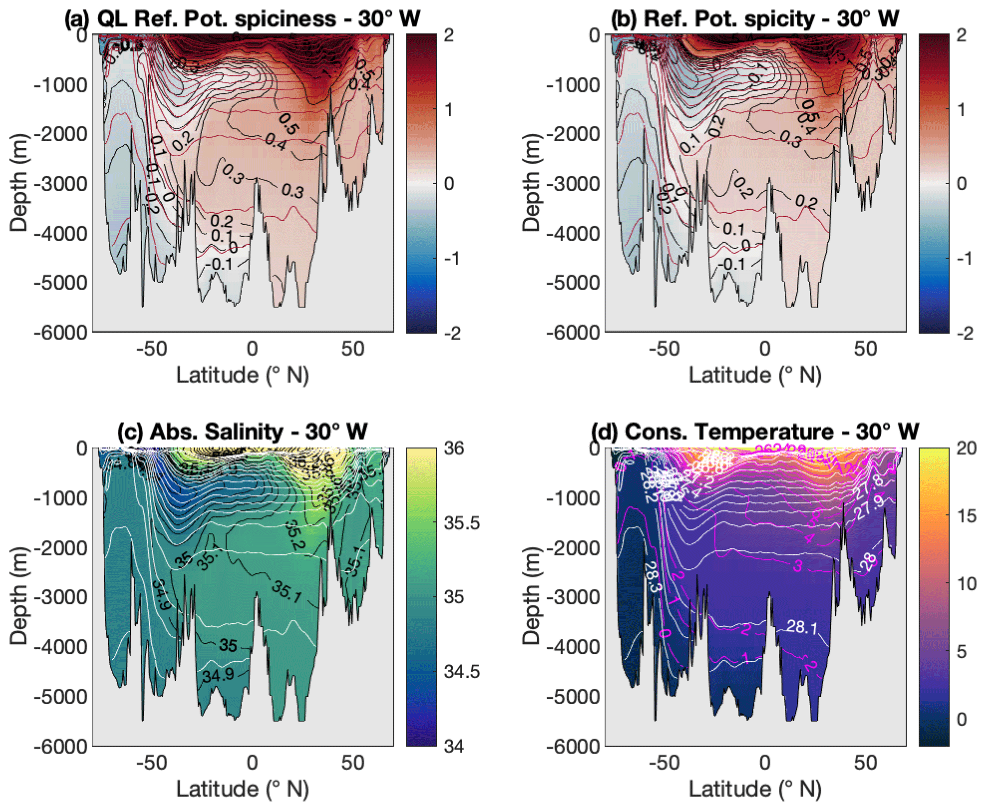
Figure 1Comparison of different spiciness as state functions along 30∘ W in the Atlantic Ocean: (a) a new form of potential spiciness referenced to a variable reference pressure pr(S,θ). This spiciness variable is similar to the McDougall and Krzysik (2015) spiciness variable and defined in Sect. 3. The variable reference pressure pr is defined in Sect. 2 and illustrated in panel (a) of Fig. 3. (b) The Huang et al. (2018) potential spicity referenced to the same variable reference pressure pr as in (a), denoted by πref in the paper; (c) Absolute Salinity; (d) Conservative Temperature. White contours in (c) and (d) (shown as brown contours in a and b) represent selected isocontours of a density-like variable similar to the Tailleux (2016b) thermodynamic neutral density variable γT. The construction and implementation of are described in Sect. 2. These isocontours – the same in all panels – are only labelled in (d) for clarity.
From a purely empirical viewpoint, neither spiciness (however defined) nor Huang et al. (2018) spicity appears to have any particular advantage over salinity at picking up ocean water mass signals, although both variables are superior to temperature in this respect. This is shown in Fig. 1, which compares the aptitude of (a) reference potential spiciness τref, (b) reference potential spicity πref, (c) Absolute Salinity, and (d) Conservative Temperature for visualising the water masses of the Atlantic Ocean along the 30∘ W section, the four main ones of which are North Atlantic Deep Water (NADW), Antarctic Intermediate Water (AAIW), Antarctic Bottom Water (AABW), and Mediterranean Intermediate Water (MIW). The WOCE climatological dataset (Gouretski and Koltermann, 2004; available at: http://icdc.cen.uni-hamburg.de/1/daten/index.php?id=woce&L=1, last access: 25 January 2021) has been used for this figure and for all calculations throughout this paper. The link between τref and πref as well as the spiciness and spicity variables of McDougall and Krzysik (2015) and Huang et al. (2018) is explained in the next two sections. Figure 1 shows that while all variables are able to pick up the AABW signal similarly well, they differ in their ability to pick up the AAIW signal. Indeed, AAIW is most prominently displayed in the salinity field, followed by πref and τref, with Conservative Temperature a distant last, based on how well defined the signal is and how far north it can be tracked. In regards to NADW and MIW, they can be clearly identified in all variables but temperature.
Since salinity satisfies neither form of orthogonality, it is natural to ask which properties make it superior to spiciness and spicity as a water mass indicator. Because two signals are visually most easily contrasted when their respective isocontours are orthogonal to each other, it is natural to ask whether salinity could owe its superiority to being on average more orthogonal to density than other variables in physical space. To test this, the median angle between ∇γ and ∇ξ estimated for all available points of the WOCE dataset was chosen as an orthogonality metric and computed for the four spiciness as state functions (ξ) considered. The result is displayed in Fig. 2 (represented by the blue bars) for both the global ocean (top panel) and the 30∘ W Atlantic section only (bottom panel). The median angle between ∇γ and ∇ξ was favoured over other metrics of orthogonality owing to its ability to rank the spiciness as state functions in the same order as the subjective visual determination of their ability as water mass indicators based on Fig. 1, with salinity first, πref second, τref third, and temperature last. In this paper, this idea will be further explored by investigating whether the generally observed superior ability of ξ′ over ξ as a water mass indicator can be attributed to its increased orthogonality to γ. (The results turn out to be inconclusive.)
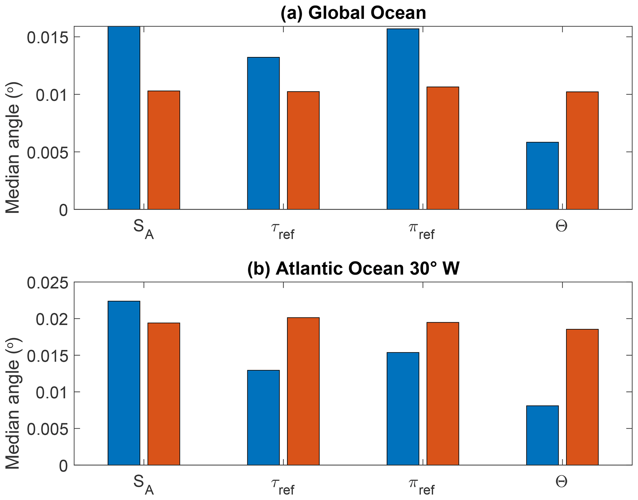
Figure 2Median angle between and ∇ξ (blue bars) as well as between and ∇ξ′ (red bars) for ξ=SA, ξ=τref, ξ=πref, and ξ=Θ. Panel (a) takes into account all available data points of the WOCE dataset, whereas (b) only accounts for the data points making up the 30∘ W Atlantic Ocean section. See Sect. 4 for details of the construction of ξ′. While the orthogonality to density of spiciness as state functions depends sensitively on the variable considered (blue bars), this is much less the case of the corresponding spiciness as anomalies, as seen by the similar magnitude exhibited by the red bars.
The main aim of this paper is to explore the above ideas further and to clarify their inter-linkages. One of its key points is to emphasise that spiciness is a property, not a substance, and hence that it is spiciness as an anomaly rather than spiciness as a state function that is the relevant concept to quantify water mass contrasts. This important point was recognised early on by Jackett and McDougall (1985) and McDougall and Giles (1987) but for some reason has since been systematically overlooked in most of the recent spiciness theory literature devoted to the construction of dedicated spiciness-as-a-state-function variables; e.g. Flament (2002), McDougall and Krzysik (2015), Huang (2011), and Huang et al. (2018). This is problematic because it has resulted in a disconnect between spiciness theory and its applications. Section 2 emphasises the result that it is the degree of neutrality of the density variable γ serving to define density-compensation that determines the degree of dynamical inertness of spiciness variables ξ, not the properties of ξ itself. Because the Tailleux (2016b) thermodynamic neutral density γT is currently the most neutral material density-like variable available, a new implementation of it, denoted , is proposed for use in spiciness studies. In contrast to γT, can be estimated with only a few lines of code and is therefore much simpler to use in practice, while also being smoother and somewhat more neutral than γT. Because relies on the use of a non-constant reference pressure field pr(S,θ), it can only be used in conjunction with spiciness as state functions whose dependence on pressure is sufficiently detailed. While this is the case of the Huang et al. (2018) spicity variable, this is not the case of the McDougall and Krzysik (2015) spiciness variable, which is only defined for three discrete reference pressures, namely 0, 1000, and 2000 dbar. To remedy this problem, Sect. 3 discusses the construction of a mathematically explicit spiciness variable , which closely mimics the behaviour of the McDougall and Krzysik (2015) variable in most of (S,θ) space. As a result, two new potential spiciness and spicity variables referenced to the non-constant reference pressure pr(S,θ), denoted by τref and πref, respectively, are introduced in this paper. These are the variables depicted in Fig. 1a and b. Section 4 discusses the links between the zero of spiciness, the definition of a notional spiceless ocean, the construction of spiciness anomalies, the orthogonality to density in physical space, and whether it is possible to meaningfully compare the spiciness of two water samples that do not belong to the same density surface. Finally, Sect. 5 summarises the results and discusses their implications and any further work needed.
2.1 Dynamical inertness of spiciness and neutrality
As mentioned above, density-compensated thermohaline variations are truly passive only if defined along surfaces of constant in situ ρ. However, because such surfaces are sensitive to pressure variations, it is useful in practice to seek a purely material proxy of in situ density, which can also be used to capture the active part of S and θ. By introducing an as yet undetermined additional spiciness as a state function, ξ, to capture the passive part of S and θ, in situ density may thus be rewritten as a function of the new coordinates as , with a hat being used for the representation of any function of . By using the so-called Jacobi method (see e.g. Appendix A of Feistel, 2018), Tailleux (2016a) showed that the partial derivatives of with respect to γ and ξ are given by
where , , and . To clarify the conditions controlling the passive character of ξ, it is useful to derive the following expression for the neutral vector N in coordinates:
where , , and . Because the Jacobian J is invariant upon the transformation , the expression for N may alternatively be written in terms of ∇γ and as follows:
Physically, the condition for ξ or ξ′ to be dynamically inert is that it does not affect , which mathematically requires . Equations (3) and (4) show this is equivalent to γ being exactly neutral. Equation (2) shows that this can only be the case if . As is well known, this condition can never be completely satisfied in practice because of thermobaricity, i.e. the pressure dependence of the thermal expansion coefficient (McDougall, 1987; Tailleux, 2016a). The above conditions thus establish that the degree of dynamical inertness of ξ is controlled by the degree of non-neutrality of γ. This is an important result for two reasons. First, it shows that the degree of dynamical inertness of ξ is not determined by its properties (such as orthogonality) but by those of γ. Second, it provides new rigorous theoretical arguments for justifying the pursuit of a globally defined material density variable γ(S,θ) maximising neutrality (although this will not come as a surprise to most oceanographers).
2.2 A new implementation of thermodynamic neutral density for spiciness studies and water mass analyses
Until recently, isopycnal analysis in oceanography has relied on two main approaches: the use of vertically stacked potential densities referenced to a discrete set of reference pressures “patched” at the points of discontinuity following Reid (1994), also called patched potential density (PPD), and the use of empirical neutral density γn proposed as a continuous analogue of patched potential density by Jackett and McDougall (1997). Neither variable is exactly material, however. For PPD, this is because the points of discontinuities at which potential density is referenced to different reference pressures are a source of non-materiality; see deSzoeke and Springer (2009). For γn, this is because such a variable also depends on horizontal position and pressure, although a way to remove the pressure dependence was recently proposed by Lang et al. (2020).
Recently, Tailleux (2016b) pointed out that Lorenz reference density that enters Lorenz (1955) theory of available potential energy (APE) (see Tailleux, 2013b for a review) could be viewed as a generalisation of the concept of potential density referenced to the pressure pr(S,θ) that a parcel would have in a notional reference state of rest. A computationally efficient approach to estimate the reference density and pressure vertical profiles ρ0(z) and p0(z) that characterise the Lorenz reference state was proposed by Saenz et al. (2015). Once the latter are known, the reference pressure pr=p0(zr) is simply obtained by solving the Tailleux (2013a) level neutral buoyancy (LNB) equation,
for the reference depth zr. As it turns out, ρLZ happens to be quite neutral away from the polar regions where fluid parcels are close to their reference position. However, like in situ density, ρLZ is dominated by compressibility and its dependence on pressure. Tailleux (2016b) defined the thermodynamic neutral density variable,
as a modified form of Lorenz reference density empirically corrected for pressure and realised that the empirical correction function f(pr) could be chosen so that γT closely approximates Jackett and McDougall (1997) empirical neutral density γn outside the ACC1.
Thermodynamic neutral density γT is attractive because it is as far as we know the most neutral purely material density-like variable around. Unlike PPD, it varies smoothly and continuously across all pressure ranges. Moreover, it also provides a non-constant reference pressure pr(S,θ) that can serve to define potential spiciness and potential spicity variables possessing the same degree of smoothness as γT, whose construction is discussed in Sect. 3. At present, γT is therefore the most natural choice for use in spiciness studies since γn, which, although somewhat more neutral, is not purely material. However, the Tailleux (2013b) original implementation of γT is a multi-step process starting with the computation of the Lorenz reference state, which, although made relatively easy by the Saenz et al. (2015) method, is computationally involved and therefore not necessarily easily reproducible by others. To circumvent these difficulties, I am proposing here an alternative construction of γT, called , which by contrast is easily computed with only a few lines of code while also being smoother and somewhat more neutral than γT. The proposed approach relies on using analytic profiles for ρ0(z) and p0(z) instead of determining these empirically, given by
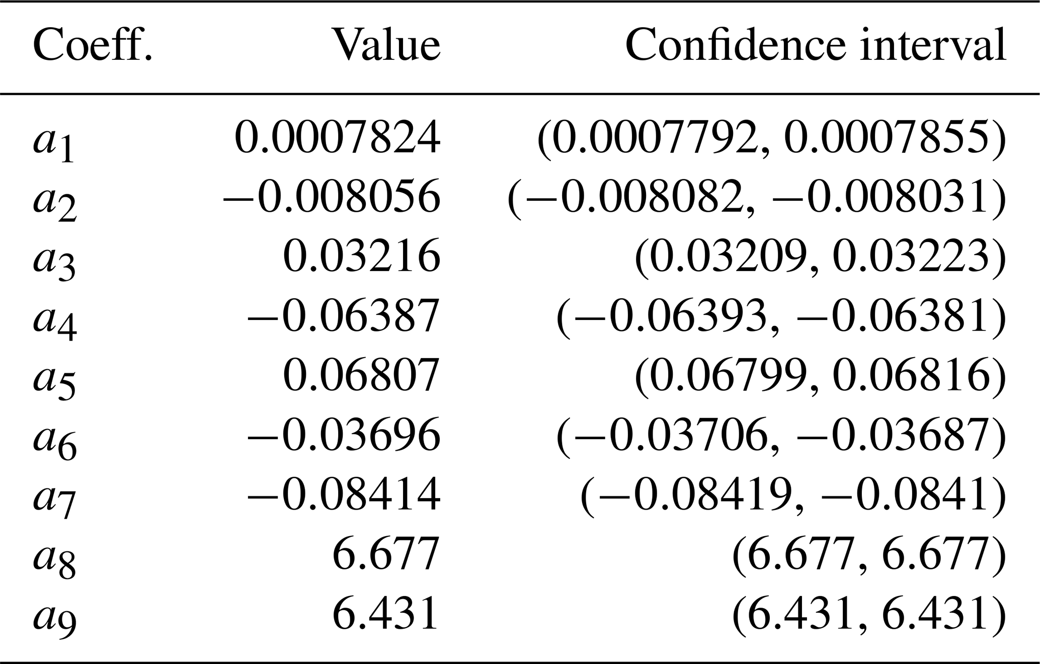
where z is positive depth increasing downward. The reference density profile ρ0(z) depends on five parameters , which were estimated by fitting the top-down Lorenz reference density profile of Saenz et al. (2015). The results of the fitting procedure are given in Table A1. As to the empirical pressure correction f(p) entering Eq. (6), it is chosen as a polynomial of degree 9 of the normalised pressure and given by the following expression:
The values of the coefficients an, pm, and Δp, as well as estimates of confidence intervals returned by the fitting procedure are given in Appendix A.
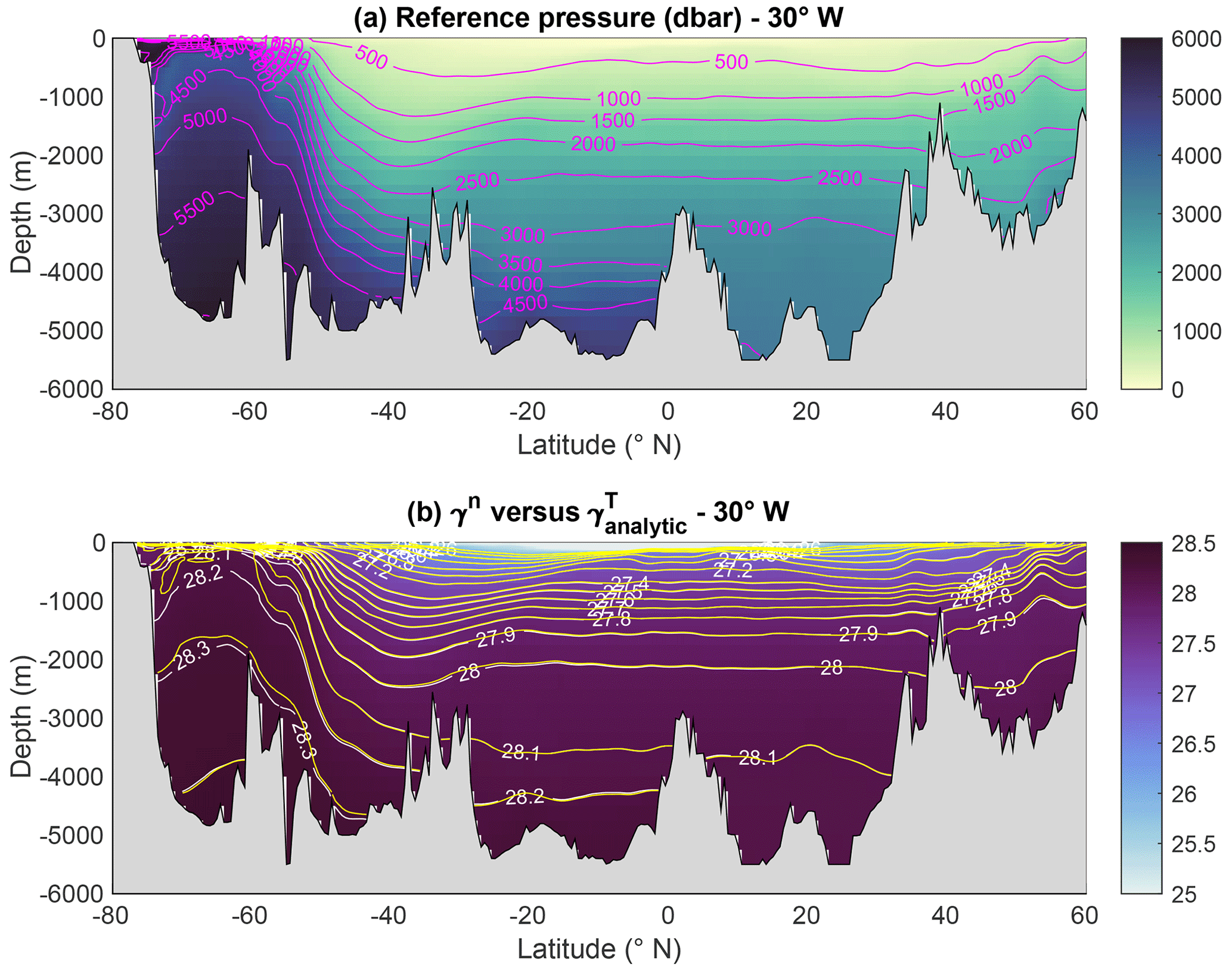
Figure 3(a) Atlantic section along 30∘ W of the variable reference pressure used for the construction of potential spiciness . (b) Atlantic section along 30∘ W of the Jackett and McDougall (1997) empirical neutral density variable γn. The white labelled contours represent selected isolines of γn, while the unlabelled yellow contours represent the same isolines but for .

Figure 4Atlantic sections along 30∘ W of the effective diffusivity of (a) the Jackett and McDougall (1997) empirical neutral density γn, (b) analytic thermodynamic neutral density , (c) potential density σ1, and (d) potential density σ2. The white masked areas flag regions where m2 s−1, which is widely used as a threshold indicating large departure from non-neutrality. These show that is in general significantly more neutral than standard potential density variables, while it is also similarly neutral as γn north of 50∘ S.
A full account of the performances and properties of will be reported in a forthcoming paper and is therefore outside the scope of this paper. Here, I only show two illustrations that are sufficient to justify the usefulness of for the present purposes. Thus, the top panel of Fig. 3 depicts the reference pressure field along 30∘ W in the Atlantic Ocean, while the bottom panel demonstrates the very close agreement between γT and γn outside the Southern Ocean along the same section (the calculations presented actually make use of the new thermodynamic standard and use Absolute Salinity SA and Conservative Temperature Θ; see Pawlowicz et al., 2012; IOC et al., 2010). Similarly good agreement was also verified in other parts of the ocean (not shown). Figure 4 depicts latitude–depth sections along 30∘ W in the Atlantic Ocean of the effective diffusivity introduced by Hochet et al. (2019), a metric for the degree of non-neutrality similar to the concept of fictitious diffusivity used by Lang et al. (2020) and others, for (a) γn, (b) , (c) σ1, and (d) σ2. As before, N is the neutral vector, γ the density-like variable of interest, and (N,∇γ) the angle between N and ∇γ. The effective diffusivity Kf is conventionally defined using Ki=1000 m2 s−1, a notional isoneutral turbulent mixing coefficient typical of observed values. It has become conventional to use the value m2 s−1 as the threshold separating acceptable from annoyingly large degrees of non-neutrality. By this measure, Fig. 4b shows that unlike σ1 and σ2, the degree of neutrality of is uniformly acceptable everywhere in the water column north of 50∘ S, where it is comparable to that of γn. How to adapt the McDougall and Krzysik (2015) and Huang et al. (2018) potential spiciness and spicity variables to be consistent with is discussed in the next section.
Since spiciness is a water mass property that can a priori be measured in terms of the isopycnal variations of any arbitrary function ξ(S,θ) independent of density, an important question in spiciness theory is whether there is any real physical justification or benefits for introducing the kind of dedicated spiciness as state functions discussed by Veronis (1972), Jackett and McDougall (1985), Flament (2002), McDougall and Krzysik (2015), Huang (2011), and Huang et al. (2018). Assuming that this is the case, how can existing spiciness and spicity variables be adapted to be used consistently with and the non-constant reference pressure pr(S,θ) defined in the previous section, given that existing codes for computing such variables are in general limited to a few discrete reference pressures?
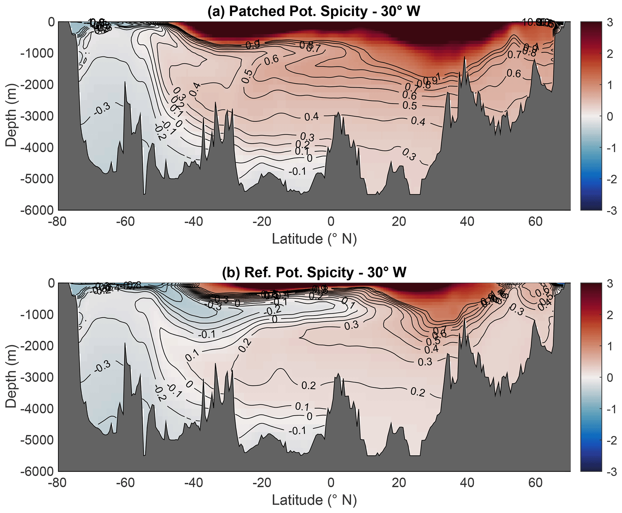
Figure 5(a) Patched potential spicity referenced to the relevant reference pressure appropriate to the pressure range of fluid parcels; (b) potential spicity referenced to the variable reference pressure pr(SA,Θ). Referencing potential spicity to the variable reference pressure pr significantly increases its ability as a water mass indicator, especially with respect to the representation of AAIW.
3.1 Mathematical problems defining spiciness as state functions
To examine the benefits that might be attached to a particular choice of spiciness as a state function ξ(S,θ) for studying water mass contrasts, it is useful to establish some general properties about what controls its isopycnal variations. By denoting di the restriction of the total differential operator to an isopycnal surface γ=constant, the isopycnal variations of the latter may be written in the following equivalent forms:
where , , , and using the fact that by construction , with being the Jacobian of the transformation as before. Equation (10) establishes the following.
-
diξ is proportional to the elemental imperfect differential with proportionality factor for all spiciness as state functions, ξ. The two quantities γSdiS and γθdiθ have the same physical units; they can thus be regarded as the basic building blocks for the construction of any spiciness-as-state-function variable if so desired.
-
diξ is unaffected by the transformation , where ξr(γ) is any arbitrary function of γ, so that both ξ and ξ−ξr(γ) have identical isopycnal variations. The benefit of imposing some particular property on ξ, such as orthogonality to γ, is therefore not obvious since such a property cannot in general be satisfied by both ξ and ξ−ξr(γ).
According to Eq. (10), the main quantity determining the properties of the spiciness as a state function ξ is the Jacobian J. The generic mathematical problem determining ξ may therefore be written in the form
Eq. (11) can be recognised as a standard quasi-linear partial differential equation amenable to the method of characteristics. Its general solution is defined up to some function ξr(γ) depending on the boundary conditions imposed ξ. In the important particular cases in which ξ=θ and ξ=S, the Jacobian and amplification factors are given by
Eqs. (12) and (13) exemplify the two main kinds of behaviour of spiciness as state functions. For salinity-like ξ, the Jacobian varies as γθ and is therefore quite non-uniform, with loss of invertibility where γθ=0; however, the scaling factor varies as and therefore varies little in (S,θ) space. This is the opposite for temperature-like ξ, for which it is the Jacobian that is approximately constant and the scaling factor that varies non-uniformly. To a large extent, these opposing behaviours characterise the McDougall and Krzysik (2015) and Huang et al. (2018) spiciness and spicity variables. Which behaviour is preferable cannot be determined without bringing in additional physical considerations discussed in Sect. 4 and the Conclusions.
3.2 Construction of reference potential spicity πref
The Huang et al. (2018) spicity variable π(SA,Θ) is designed to enforce the Veronis (1972) definition of orthogonality in the re-scaled SA and Θ coordinates X(SA)=ρ0β0SA and Y(Θ)=ρ0α0Θ, with α0 and β0 being representative constant values of the thermal expansion and haline contraction coefficients, respectively. The imposition of this form of orthogonality ensures that the transformation is invertible everywhere in (SA,Θ) space, which is not the case of the 45∘ form of orthogonality considered by Jackett and McDougall (1985), Flament (2002), and McDougall and Krzysik (2015). Huang et al. (2018) provide a MATLAB subroutine, gsw_pspi(SA,CT,pr), to compute π as a function of Absolute Salinity and Conservative Temperature at the discrete set of reference pressures pr=0, 500, 1000, 2000, 3000, 4000, and 5000 dbar. This provides sufficient vertical resolution for computing the reference potential spicity referenced to the variable reference pressure pr(SA,Θ) defined in the previous section using shape-preserving spline interpolation, as illustrated in Fig. 5b. By comparison, panel (a) shows the patched potential spicity obtained by stacking up potential spicity estimated at the reference pressure appropriate to its pressure range (which appears to be smoother than might have been expected, given the six transition points of discontinuities at p=250, 750, 1500, 2500, 3500, and 4500 dbar). This shows that the use of the variable reference pressure pr(SA,Θ) has a dramatic impact on the ability of spicity to pick up the water mass signals of the Atlantic Ocean. This is especially evident for the AAIW signal, which is only vaguely apparent in patched potential spicity, while being nearly as well defined in πref as in the salinity field. This suggests that it is more advantageous to use potential spicity with than with patched potential density.
3.3 Construction of reference potential spiciness τref
The Jackett and McDougall (1985) spiciness as a state function τ is designed so that its isopycnal variations are constrained to satisfy the following mathematically equivalent relations:
where, as before, di is the restriction of the total differential operator to the isopycnal surface and where α and β are the haline contraction and thermohaline expansion coefficients. In Jackett and McDougall (1985), density surfaces are approximated in terms of σ0, but the use of patched potential density is implicit in the more recent paper by McDougall and Krzysik (2015). By comparing Eq. (14) with Eq. (10), it can be seen that the Jackett and McDougall (1985) construction implies a constant proportionality factor . This in turn implies for the Jacobian and quasi-linear PDE satisfied by τ
To solve the quasi-linear PDE Eq. (15), Flament (2002) and Jackett and McDougall (1985) further imposed τ to satisfy the so-called 45∘ orthogonality, which in practice amounts to assuming that the total differential of τ satisfies ), with λ being some integrating factor. Flament (2002) and Jackett and McDougall (1985) approached the problem somewhat differently, but their variables are nevertheless approximately linearly re-scaled functions of each other.
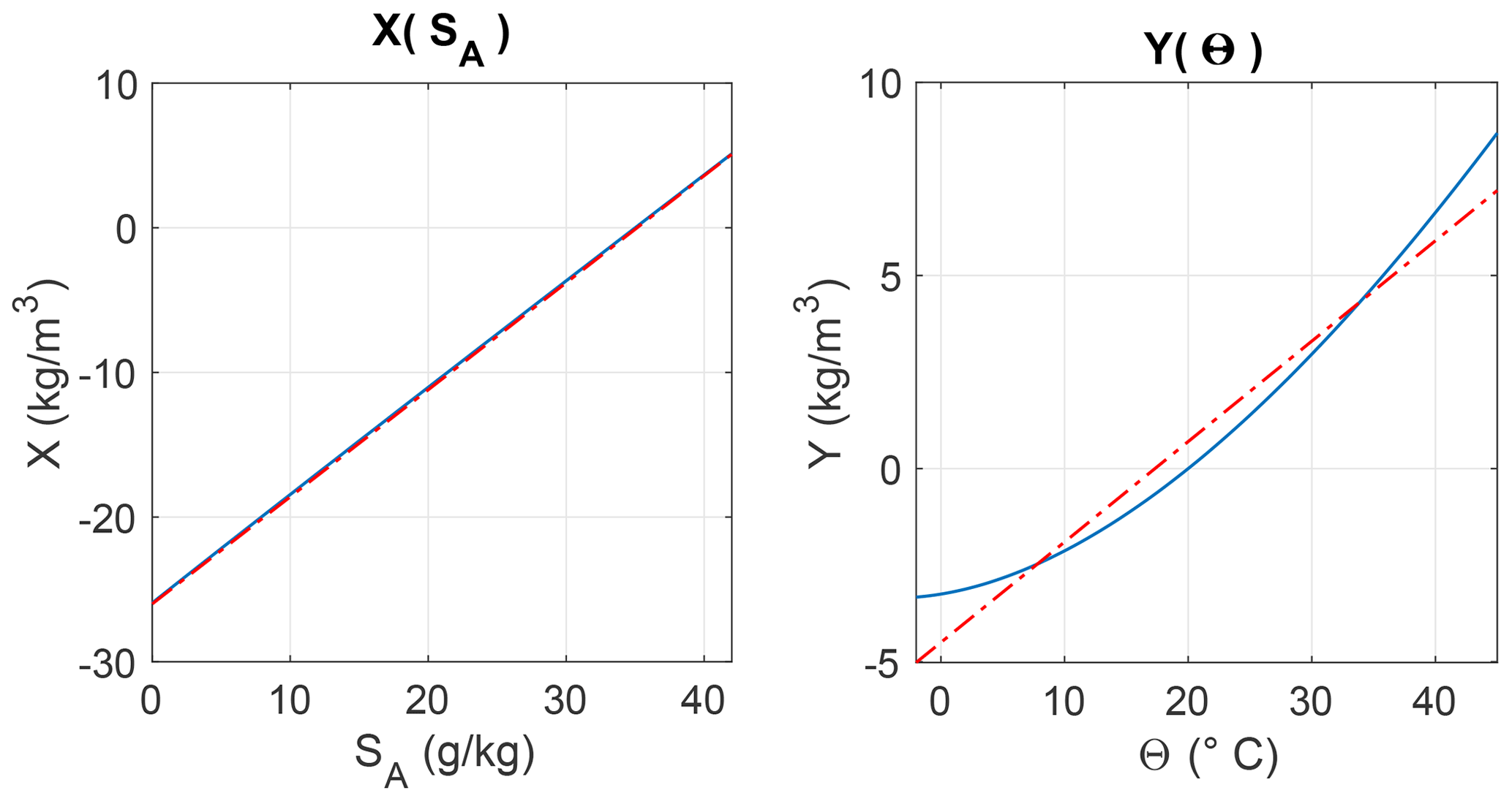
Figure 6The re-scaled salinity and temperature X(SA) and Y(Θ) expressing both quantities in a common system of density-like units. Red dashed lines are the linear regressions of the equations and .
Both Jackett and McDougall (1985) and Flament (2002) provide polynomial expressions in powers of S and θ for their potential spiciness variable, which are, however, limited to a single reference pressure pr=0. More recently, McDougall and Krzysik (2015) have provided the MATLAB subroutines (available at http://www.teos-10.org, last access: 25 January 2021) gsw_spice0(SA,CT), gsw_spice1(SA,CT), and gsw_spice2(SA,CT) to compute potential spiciness at the three reference pressures pr=0 dbar, pr=1000 dbar, and pr=2000 dbar, where SA is absolute salinity and CT conservative temperature. Because this limited number of reference pressures is far from ideal for computing potential spiciness referenced to the variable reference pressure pr(SA,Θ) underlying , I have constructed an analytical proxy for the McDougall and Krzysik (2015) variable valid for the full range of pressures encountered in the ocean. The expression for this proxy, called quasi-linear spiciness, is
τ‡ is a linear combination of the non-linear re-scaled salinity and temperature coordinates X(S,p) and Y(θ,p) and of reference function τ0(p), whose expressions are
These functions depend on some arbitrary reference constants, specified as follows: ρ00=1000 kg m−3 is chosen to give τ‡ the same unit as density, while specifies the reference value of τ‡ at the reference point (S0,θ0). In principle, S0 and θ0 could also be made to depend on pressure p, but this complication is avoided for simplicity. Figure 6 illustrates a particular construction of X(SA,p) and Y(Θ,p) based on the values S0=35 g kg−1, Θ0=20 ∘C, and p=0 dbar. The reference point (Sref,θref) defines where τ‡ vanishes. The values Sref=35.16504 g kg−1 and Θref=0 ∘C were used to fix the zero of τ‡ as in McDougall and Krzysik (2015). Figure 6 shows that while Y(SA) varies approximately linearly with SA, Y(Θ) clearly varies non-linearly with Θ. Linear regression lines are also indicated to illustrate the departure from non-linearity. The total and isopycnal differentials of potential spiciness referenced to the constant reference pressure pr are
where and . For (S,θ) close enough to the reference point (S0,θ0), diτ‡≈2ρ00βdiS, which is equivalent to the differential problem that Jackett and McDougall (1985) set out to solve. An important difference with standard spiciness variables, however, is that the Jacobian associated with τ‡ is given by
and it differs from zero everywhere in (S,θ) space. As to the pressure dependence of τ‡, it is given by
where . Equation (21) shows that ∂pτ‡ vanishes at the two reference points (S0,θ0) and (Sref,θref); it follows that, by design, τ‡ is only weakly dependent on pressure and hence naturally quasi-material (that is, approximately conserved following fluid parcels in the absence of diffusive sources and sinks of S and θ).
The McDougall and Krzysik (2015) spiciness and τ‡ are compared in Figs. 7 and 8 in (SA,Θ) space as well as in the re-scaled (X,Y) coordinates, respectively, at the reference pressure pr=0. The two variables can be seen to behave in essentially the same way, with the result also holding at pr=1000 dbar and pr=2000 dbar, except for cold temperature and low salinity values at which the Jacobian associated with McDougall and Krzysik (2015) spiciness vanishes, while that associated with τ‡ does not. That both variables approximately satisfy the 45∘ orthogonality is made obvious in the re-scaled (X,Y) coordinates in Fig. 8; interestingly, this plot suggests that in situ density is approximately a linear function of X and Y, which is further examined in Appendix B. Moving to physical space, Fig. 9 compares the patched potential spiciness computed using the McDougall and Krzysik (2015) software (top panel) versus the reference potential spiciness calculated with τ‡. For patched potential spiciness, the transition points of discontinuity were chosen at pr=1000 and 2000 dbar. As for potential spicity, it also appears to be advantageous to use potential spiciness with a variable pr, as it makes AAIW more marked and NADW somewhat more homogeneous. The effect of a variable pr on potential spiciness is not as dramatic as for potential spicity, however, which is likely due to the weak pressure dependence of τ‡ noted above. In any case, the above analysis suggests that τ‡ is a useful proxy for the McDougall and Krzysik (2015) spiciness variable.
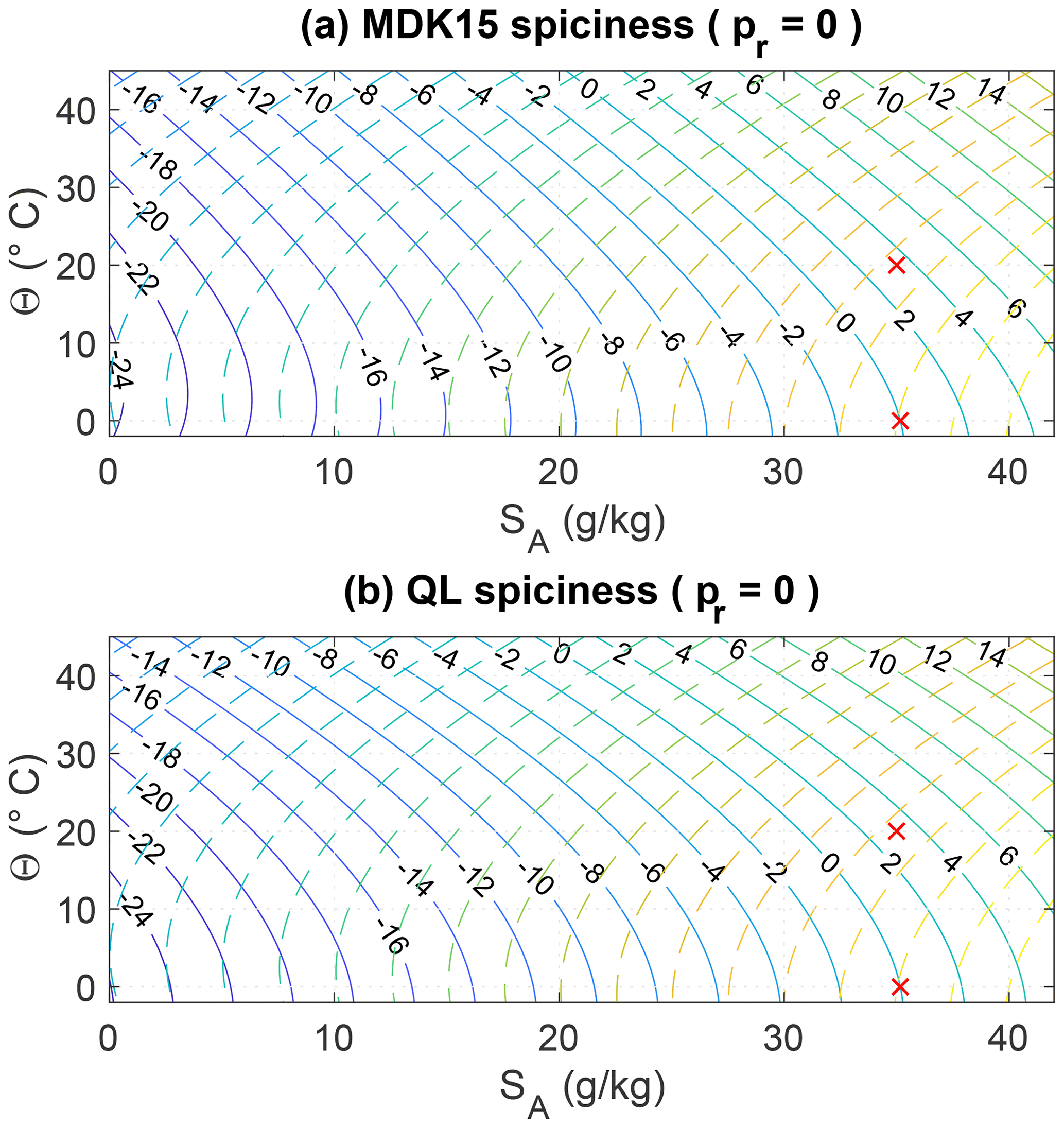
Figure 7(a) Isocontours of the McDougall and Krzysik (2015) spiciness variable referenced to the surface pressure (solid lines) along with σ0 isocontours (dashed lines). (b) Isocontours of the mathematically explicit quasi-linear spiciness variable introduced in this paper referenced to the surface pressure (solid lines) along with σ0 isocontours (dashed lines). The crosses indicate the reference point at which and the reference point at which both spiciness variables are imposed to vanish.
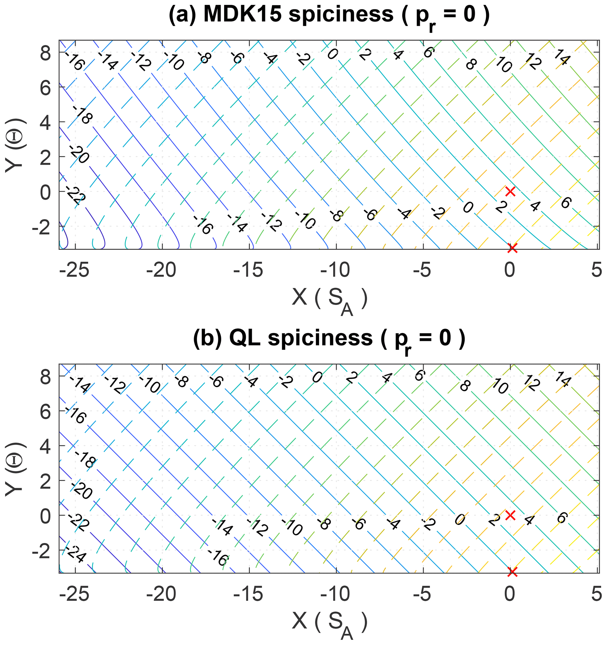
Figure 8Same as Fig. 7 but with SA and Θ replaced by the re-scaled salinity and temperature coordinates X(SA) and Y(Θ), in which the spiciness and density variables visually appear approximately orthogonal to each other.
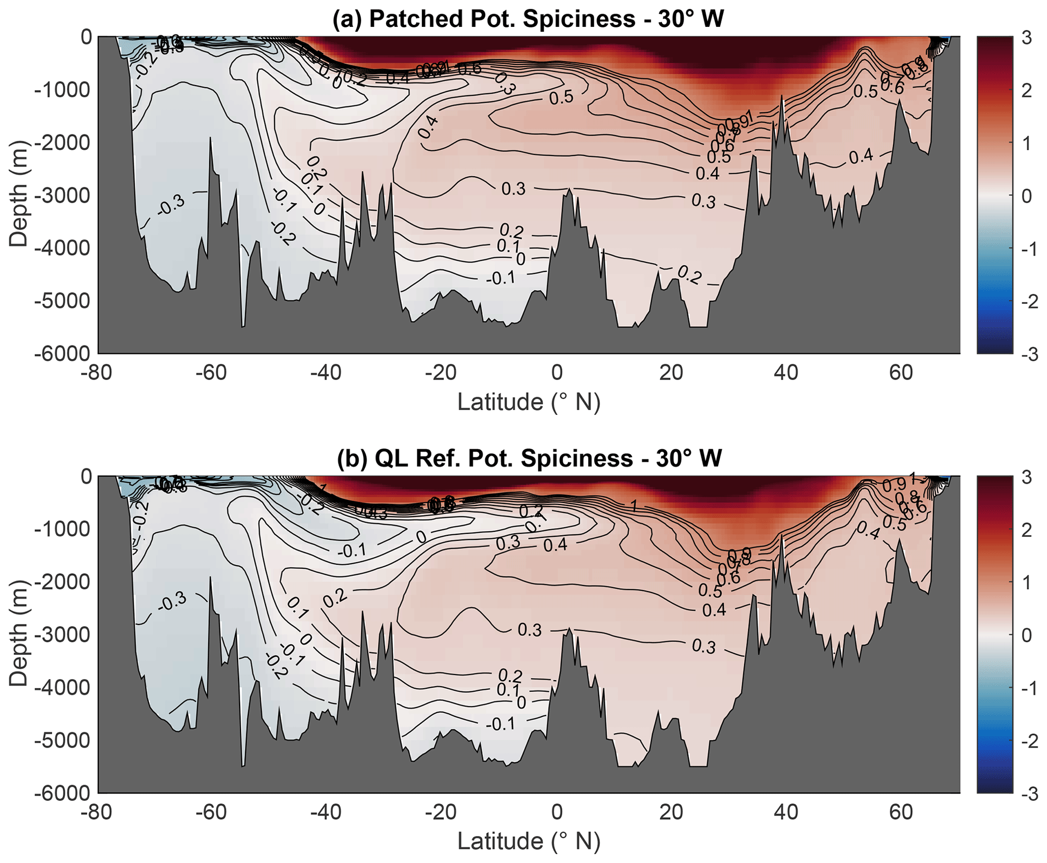
Figure 9(a) Patched potential spiciness referenced to the three discrete reference pressures provided by the McDougall and Krzysik (2015) software appropriate to their pressure ranges. (b) Quasi-linear potential spiciness referenced to the variable reference pressure . In contrast to spicity, the use of a variable reference pressure has little impact on the visual aspect of spiciness, thus confirming the weak pressure dependence of .
As stated previously, it is important to recognise that spiciness is not a substance but a property that cannot be described without taking into account empirical information about the particular water masses to be analysed. Whether this point is well known is unclear because the distinction between a property and a substance is rarely evoked if ever in the spiciness literature. As a result, it follows that the usefulness of spiciness-as-a-state-function variables such as those of Jackett and McDougall (1985), Flament (2002), and Huang et al. (2018), which do not incorporate any information about the particular water masses to be analysed, is only limited to quantifying the relative differences in spiciness for fluid parcels that belong to the same density surface, as pointed out Timmermans and Jayne (2016). In other words, any difference in spiciness for fluid parcels belonging to different density surfaces predicted by such variables is physically meaningless. Physically, this limitation is associated with another key one, namely the impossibility to link a spiceless ocean to the zero value of a spiciness-as-a-state-function variable. This is not surprising because the zero and other isovalues of any spiciness as a state function are necessarily artificial since they are not informed by a physical consideration of how to endow the relative spiciness of two fluid parcels that belong to different density surfaces with physical meaning. Here, a spiceless ocean is defined as a notional ocean in which iso-surfaces of potential temperature, salinity, and potential density would all coincide. It follows that in a spiceless ocean, any spiciness as a state function would have to be a function of density only, for example ξ=ξr(γ), which in general must differ from zero. This suggests that spiciness as a property should be defined as the anomaly , as originally proposed by Jackett and McDougall (1985) and McDougall and Giles (1987). Clearly, such an approach addresses the zero-of-spiciness issue, since it ensures that ξ′ would vanish in a spiceless ocean, as desired. Moreover, it also define spiciness as a property rather than as a substance because although is a function of S and θ, it is not truly a function of state owing to its dependence on the empirically determined function of density ξr(γ).
Because any function ξ(S,θ) independent of γ is a potential candidate for constructing a spiciness-as-a-property variable, the following questions arise.
-
Are there any benefits in constructing a dedicated spiciness as a state function ξ for the purpose of constructing the anomaly ? Are there any good reasons to think that and are not suitable or insufficient for all practical purposes?
-
Since neither the Veronis (1972) form of orthogonality nor the Jackett and McDougall (1985) 45∘ orthogonality can be satisfied by ξ′, what is the physical justification for imposing it on ξ in the first place?
-
In physics, the scale to measure some quantities is commonly accepted to be arbitrary, which is why several scales (e.g. Kelvin, Celsius, and Fahrenheit) have been developed over time to measure temperature, for instance. To what extent is the problem of quantifying spiciness as a property similar to or different from that of constructing a temperature scale?
-
To what extent is the problem of deciding in favour of a particular choice of ξ one that can be constrained by physical arguments as opposed to one that is fundamentally arbitrary and therefore a matter of personal preference?
-
Are there any additional constraints that should satisfy beyond the zero-of-spiciness issue in order for relative difference in ξ′ for fluid parcels that belong to different density surfaces to be considered physically meaningful?
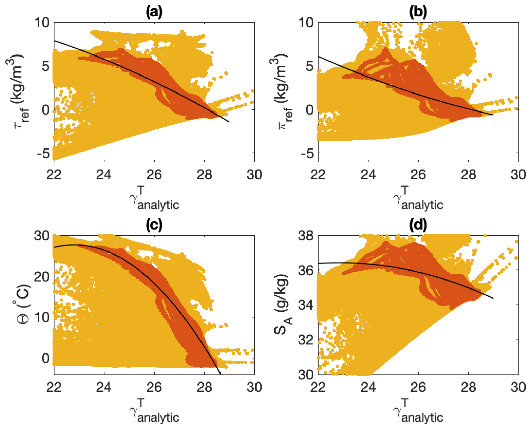
Figure 10Non-linear regression between and various spiciness as state functions estimated for data restricted to the 30∘ W Atlantic section (in red and orange): (a) potential reference spiciness τref, (b) potential reference spiciness πeref, (c) Conservative Temperature, and (d) Absolute Salinity. The non-linear regression curve is indicated in solid black and is described by a second-order polynomial in . The yellow data points represent the whole dataset for the global ocean for comparison.
Jackett and McDougall (1985) shed some light on some of the above issues by suggesting that the choice of ξ may be less important than one would think. Indeed, they showed that the inter-differences in appropriately re-scaled anomaly functions , , and S′ were considerably reduced over those exhibited by τjmd, τν, and S, a potentially important result that does not appear to have received much attention so far. The Jackett and McDougall (1985) conclusion is only based on the comparison of two vertical soundings, however, so it is necessary to examine it more systematically in order to assess its robustness. To that end, I constructed particular examples of anomaly functions ξ′ for the four variables considered in the Introduction based on the use of a second-order polynomial descriptor for ξr(γ) obtained by means of a non-linear regression of ξ against . A polynomial descriptor was preferred over using a simple isopycnal average as in Jackett and McDougall (1985) or McDougall and Giles (1987) to ensure the smoothness and differentiability of . To minimise the impact of outliers, the robust bisquare least-squares provided by MATLAB was used2. Because a scatter plot of ξ against does not reveal any particular relation between the two variables if all the ocean data points are used, as shown in Fig. 10 by the yellow points, the non-linear regression for obtaining the second-order polynomial was restricted to the points making up the 30∘ W Atlantic section (indicated in red and orange), for which a relation is more apparent. The resulting function, depicted as the black solid line in Fig. 10, was then used to construct ξ′ in both thermohaline space in Fig. 11 and physical space in Fig. 12. Similarly as in Jackett and McDougall (1985), Fig. 11 shows that the significant inter-differences in behaviour exhibited by the different ξ are considerably reduced for ξ′. The result is significantly more general than in Jackett and McDougall (1985), however, since it pertains to a large part of (SA,Θ) space as opposed to being limited to a few vertical soundings. In all plots in Fig. 11, is shown to be an increasing function of SA but decreasing function of Θ, similarly as density but with a much weaker dependence on Θ. This departs from the conventional wisdom that spiciness should be an increasing function of both SA and Θ, as is the case of McDougall and Krzysik (2015) spiciness and Huang et al. (2018) spicity variables. However, this is based on only one particular construction of ξr(γ) constrained by the properties of the Atlantic Ocean, so it might not be a general result valid for all possible constructions of ξr(γ).

Figure 11Isocontours of (red and brown solid lines), ξ (dashed magenta lines), and ξ′ (black solid lines) for various spiciness as state functions, ξ: (a) reference potential spiciness τref, (b) reference potential spicity πref, (c) Absolute Salinity, and (d) Conservative Temperature. The isocontours for are the same in all panels but labels are only shown in (c) and (d).
To make them more comparable, the various ξ′ values were re-scaled by the root mean square error (RMSE) of all data points making up the 30∘ W Atlantic section before being drawn in Fig. 12. As a result of the re-scaling, the inter-differences between the different variables have been significantly reduced but some are still noticeable. For instance, panel (d) suggests that part of AAIW is entrained by the sinking of AABW, which is not really apparent in the other panels. All re-scaled variables now appear to perform equally well as water mass indicators, with all four main Atlantic water masses following similar patterns and being characterised by similar spiciness values in all plots. Thus, MIW appears to be a high-spiciness water mass with values greater than about 0.3. AAIW appears to be a very low-spiciness water mass with negative values. AABW and NADW appear to be water masses differing only by about 0.1 spiciness units, with values for AABW and NADW ranging from 0 to about 0.2 for the former and from 0.2 to about 0.3 for the latter, except for Θ′ for which it goes to about 0.2. The nature of the inter-differences between the various re-scaled ξ′ values is further clarified by plotting the variables against each other as shown in Fig. 13. Panel (c) reveals that and are essentially indistinguishable from each other; however, the other panels reveal that and are non-linear multi-valued functions of (or ). It follows that the strong similarities exhibited by all re-scaled anomaly variables in Fig. 12 hide some important fundamental differences.
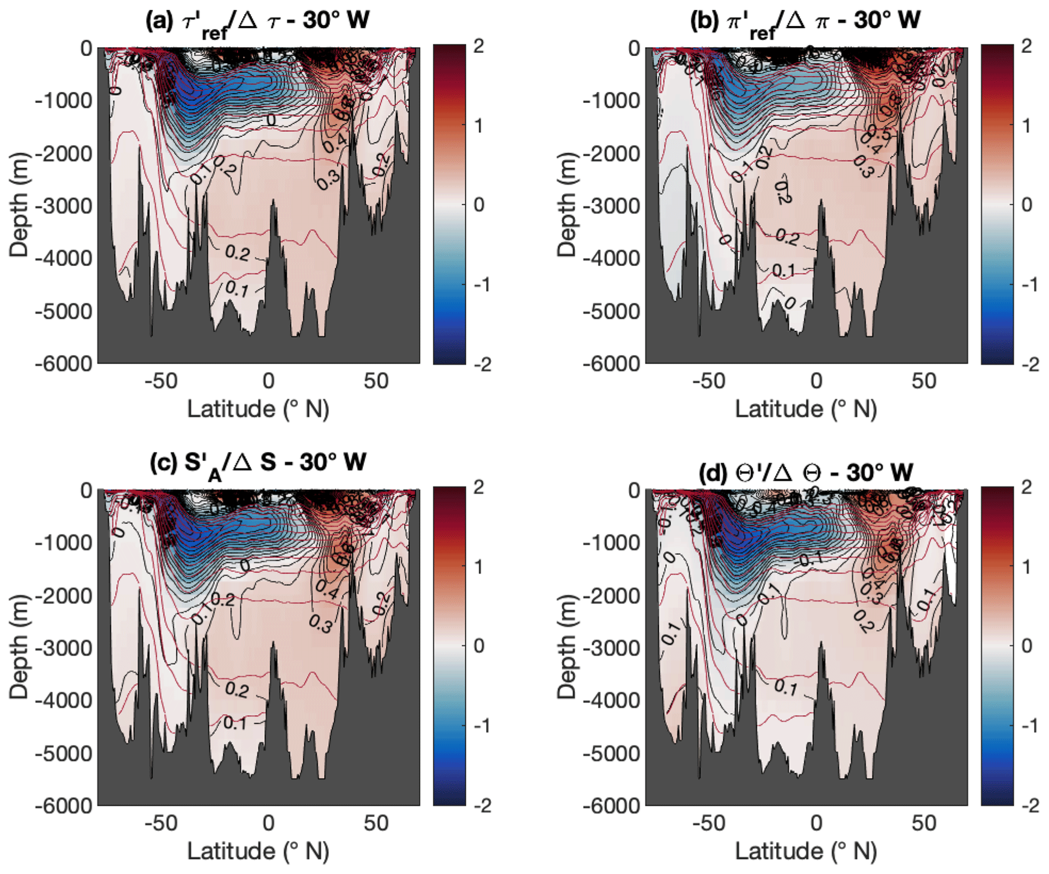
Figure 12Atlantic Ocean sections along 30∘ W of the normalised spiciness anomaly functions , with corresponding to the non-linear regression functions depicted in Fig. 10, for (a) reference potential spiciness τref, (b) reference potential spicity πref, (c) Absolute Salinity, and (d) Conservative Temperature. Brown solid lines represent the same selected isopycnal contours for as in Fig. 1. Each variable has been re-scaled by the RMSE Δξ of all data points making up this section before being drawn.
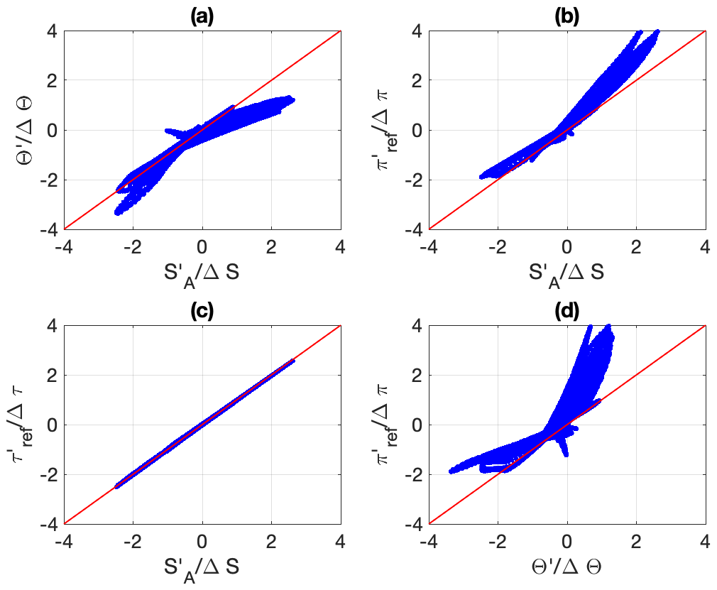
Figure 13Scatter plots of various normalised ξ′ values against each other. Panel (d) shows that is essentially equivalent to . The other panels suggest that and Θ′ behave in fundamentally different ways than and for positive and negative spiciness values.
In the Introduction, I showed that the superior ability of salinity to pick up the different water mass signals of the Atlantic Ocean3 appeared to coincide with being the most orthogonal to , with orthogonality being defined in terms of the median of all the angles between ∇ξ and estimated for all available data points. As shown in Fig. 2, such a metric ranks the various ξ values in the same order as a visual determination of their ability as water mass indicators. Since it seems clear from Fig. 12 that ξ′ systematically improves over ξ as a water mass indicator, one may ask whether this improvement can be similarly attributed to ξ′ being more orthogonal to than ξ. Figure 14 illustrates a particular idealised example for which this would be expected, as in this case ∇ξ′ can actually be imposed to be exactly orthogonal to ∇γ,
provided that ξr(γ) is chosen to satisfy
However, Fig. 2 reveals that although the orthogonality of ξ′ to is occasionally improved over that of ξ, this is not systematically the case, which suggests that the idealised case of Fig. 14 is not representative of the relative distributions of ξ and for the actual ocean water masses. In fact, the values of the median angles illustrated in Fig. 2 rarely exceed 0.02∘, which means that the isolines of ξ or ξ′ tend more often than not to make a small angle with isopycnal surfaces and that ∇ξ′ is only truly orthogonal to in a few frontal regions where two water masses collide. This is the case, for instance, where AAIW meets MIW around 20∘ N, as can be seen in Fig. 12. This therefore suggests that the angle between ∇ξ′ and ∇γ is strongly controlled by isopycnal stirring outside such frontal regions. Therefore, although the orthogonality in physical space seems more germane to spiciness theory than orthogonality in thermohaline space, how to actually make use of it to constrain ξ or ξr(γ) has yet to be fully understood and clarified.
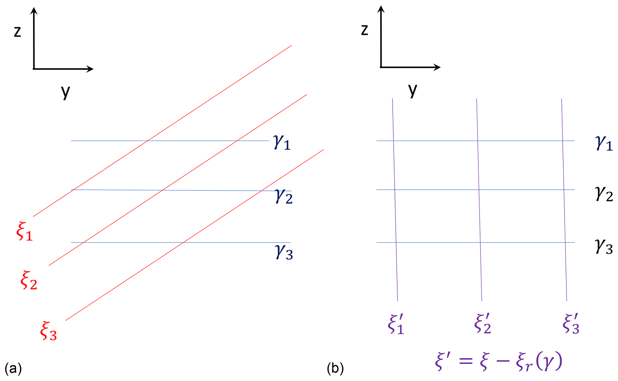
Figure 14Schematics of the effect of subtracting a suitably defined function of density γ from a spiciness as a state function, ξ. In (a), the isolines of γ and ξ are assumed to be linear functions of z such that and at an angle less than 90∘. In (b), the isolines of are described by the equation , with . This has removed the z-dependent part of ξ, resulting in ξ′ and γ being orthogonal in physical space.
In this paper, I have revisited the theory of spiciness and established that its main ingredients are (1) a quasi-material density-like variable γ(S,θ) that needs to be as neutral as feasible, (2) a quasi-material spiciness as a state function ξ(S,θ) independent of γ so that (ξ,γ) can be inverted to recover the (S,θ) properties of any fluid parcel, and (3) an empirical reference function ξr(γ) defined such that the zero value of the spiciness as a property, , describes a physically plausible notional spiceless ocean in which all surfaces of constant salinity, potential temperature, and density would coincide.
Ingredient (1) is required because, contrary to what has been assumed by some authors, it is not the properties of ξ that determines its degree of dynamical inertness but the degree of neutrality of γ, regardless of what ξ is. This result is important because it establishes the fact that the theory of spiciness is not independent of the theory of isopycnal analysis. In particular, it provides a rigorous theoretical justification for the pursuit of a globally defined material density-like variable maximising neutrality as originally proposed by Eden and Willebrand (1999) as an alternative to the Jackett and McDougall (1997) empirical neutral density variable γn. In this paper, I have proposed the use of a new implementation of the Tailleux (2016b) thermodynamic neutral density γT, which is smoother, more neutral, and computationally simpler to estimate than the original construction. As far as I am aware, this variable is currently the most neutral material density-like variable available. I also showed how to adapt McDougall and Krzysik (2015) and Huang et al. (2018) variables to construct the relevant forms of potential spiciness τref and potential spicity πref referenced to the variable reference pressure pr(S,θ) underlying the construction of γT. Interestingly, it is found that the use of pr improves both potential spicity and potential spiciness as water mass indicators, although this improvement is more evident for the former than for the latter.
One of the main key points repeatedly emphasised in this paper is that spiciness is not a substance but a property that cannot be meaningfully defined independently of the particular ocean water masses to be analysed. This is why spiciness as a property is really best measured by the anomaly rather than by the spiciness as a state function ξ, where the empirical information about the water masses analysed is encoded in the reference function ξr(γ). Although the use of spiciness anomalies was recommended early on by Jackett and McDougall (1985) and McDougall and Giles (1987) and underlies most of the literature devoted to understanding the role of spiciness in climate, it has since become completely overlooked in the most recent literature about spiciness theory in favour of the mathematical aspects pertaining to the construction of spiciness as state functions orthogonal to density; e.g. Flament (2002), McDougall and Krzysik (2015), Huang (2011), and Huang et al. (2018). This paper argues that the development of any dedicated spiciness as a state function, ξ, only makes sense if it is accompanied by a description of the reference function ξr(γ) that is needed to construct the anomaly . However, the fact that the normalised form of ξ′ does not appear to be very sensitive to the choice of ξ, as first suggested by Jackett and McDougall (1985) and illustrated by Figs. 11 and 12, combined with the fact than any form of orthogonality in (S,θ) space that may have been imposed on ξ is lost by ξ′, raises questions about the actual need for dedicated spiciness as state functions for constructing suitable water mass indicators or for studying the role of spiciness in climate.
One key advantage of ξ′ over ξ, however ξ is defined, is that a notional spiceless ocean can be associated with the zero value of ξ′, which in turn allows one to give physical meaning to differences in ξ′ for fluid parcels belonging to different density surfaces, neither of which make sense for ξ. This view is supported by Fig. 12, which shows that all the Atlantic water masses appear to have the same kind of spiciness behaviour regardless of ξ′, namely AAIW has very low spiciness and MIW has very high spiciness, while AABW and NADW have intermediate spiciness. Although differences in the way each variable represents ocean water masses exist, they tend to be rather subtle, making it hard to decide whether one variable should be regarded as superior to the others. Jackett and McDougall (1985) appear to disagree, as they have argued that the physical basis for their variable τjmd makes superior to S′ and for measuring water mass contrasts. However, they did not elaborate much on the physical meaning of this assumed superiority nor on how their claim could be independently tested. A clearer and physically more transparent way to assess the relative merits of a given ξ′ would be by establishing whether it mixes linearly or non-linearly under the action of irreversible diffusive mixing (a variable mixes linearly if the spiciness of the mixture is equal to the mass-weighted average of the individual spiciness values). If S and θ are governed by a standard advection–diffusion equation with symmetric turbulent mixing tensor K, the equation for ξ′ will be of the form
For ξ′ to mix linearly, the nonconservative production–destruction term due to its non-linearities in S and θ needs to be small. In this regard, and τref appear to be the variables in Fig. 11 that exhibit the smallest degree of non-linearity in SA and Θ, which suggests that they might be more conservative than πref and Θ′, although this remains to be checked. In this paper, ξr(γ) was defined as a second-order polynomial in γ so as to guarantee smoothness and differentiability, which is not necessarily true of ξr(γ) defined in terms of an isopycnal average, for instance. A full discussion of whether alternative ways to construct ξr(γ) might be preferable is beyond the scope of this paper. For instance, one could ask the question of whether it is possible to construct ξ and ξr(γ) so that ξ′ is as conservative as possible. Another important question is whether constraining ξ to be orthogonal to γ in thermohaline space, as pursued by McDougall and Krzysik (2015) and Huang et al. (2018), yields any special benefit for ξ′. To what extent can orthogonality in physical space be useful? Hopefully, the present work will help stimulate further research on these issues.
The values entering the definition of the reference density profile ρ0(z) are given in Table A1, whereas the coefficients for the polynomial entering the construction of are given in Table A2. Moreover, the parameters pm and Δp entering the normalised pressure are pm=1440 dbar and Δp=1470 dbar.
Table A1Coefficients for the analytical reference density profile ρ0(z).

The re-scaled salinity and temperature coordinates given by Eq. (17) make it possible to construct a quasi-linear approximation of in situ density as follows:
where so that, by construction, ρ‡=ρ at the reference point (S0,θ0) for all pressures. In situ density and its quasi-linear approximation are compared in Fig. B1 for p=0 as a function of SA and Θ (top panel) as well as of X and Y (bottom panel), with the red cross indicating the reference value (SA=35 g kg−1, Θ=20 ∘C) used in the definition of ρ‡. As expected, the accuracy of ρ‡ decreases away from the reference point but appears to be reasonable in the restricted salinity range [30, 40 g kg−1] that pertains to the bulk of ocean water masses. Interestingly, the bottom panel of Fig. B1 reveals that a significant fraction of the non-linear character of the equation of state is captured by X and Y so that ρ appears to be approximately linear in such coordinates.
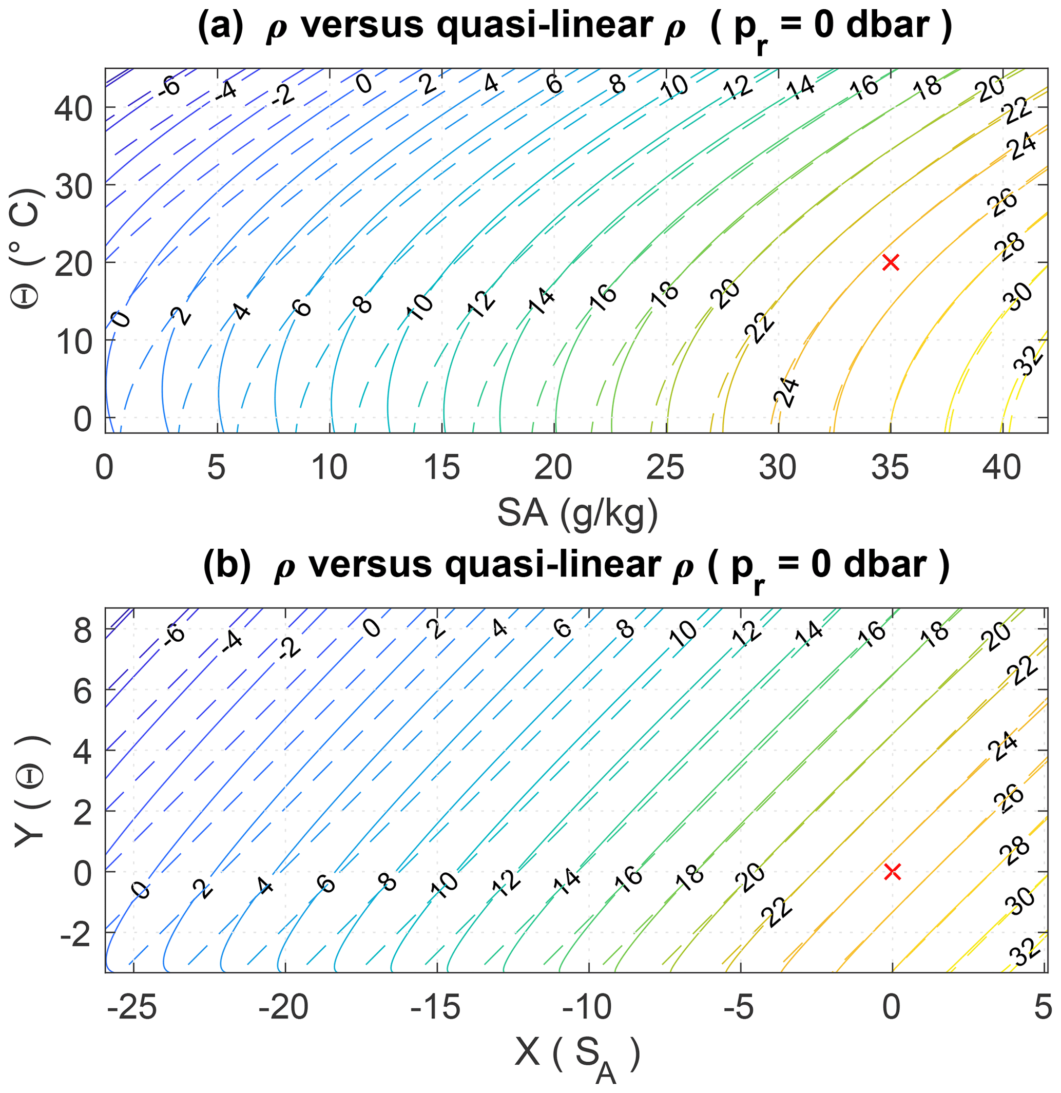
Figure B1Comparison between potential density (referenced at p=0; dbar) (solid line) and its quasi-linear approximation (dashed line), seen as a function of SA and Θ (a) as well as re-scaled coordinates X and Y (b). The red cross denotes the point at which the two functions are imposed to be equal.
The accuracy of the quasi-linear approximation ρ‡ can also be evaluated by examining how its thermal expansion, haline contraction, and compressibility compare with that of in situ density. These are given by
These relations show that the first partial derivatives of ρ‡ with respect to its three variables also coincide with their exact values at the reference point (S0,θ0), with the accuracy of the approximations decaying away from it, as expected.
MATLAB and Python subroutines for computing the variable reference pressure pr(SA,Θ) and used in this paper can be obtained by emailing the author.
The author declares that there is no conflict of interest.
The comments of Jan Zika and two anonymous reviewers, as well as the technical editing of Ilker Fer, greatly helped improving clarity of the paper and are gratefully acknowledged.
This research has been supported by the NERC-funded OUTCROP project (grant no. NE/R010536/1).
This paper was edited by Ilker Fer and reviewed by Jan Zika and two anonymous referees.
Butler, E. D., Oliver, K. I., Gregory, J. M., and Tailleux, R.: The ocean's gravitational potential energy budget in a coupled climate model, Geophys. Res. Lett., 40, 5417–5422, https://doi.org/10.1002/2013GL057996, 2013. a
deSzoeke, R. A. and Springer, S. R.: The materiality and neutrality of neutral density and orthobaric density, J. Phys. Oceanogr., 39, 1779–1799, https://doi.org/10.1175/2009JPO4042.1, 2009. a
Eden, C. and Willebrand, J.: Neutral density revisited, Deep-Sea Res., 46, 34–54, https://doi.org/10.1016/S0967-0645(98)00113-1, 1999. a, b
Feistel, R.: Thermodynamic properties of seawater, ice and humid air: TEOS-10, before and beyond, Ocean Sci., 14, 471–502, https://doi.org/10.5194/os-14-471-2018, 2018. a
Flament, P.: A state variable for characterizing water masses and their diffusive stability: Spiciness, Prog. Oceanogr., 54, 493–501, https://doi.org/10.1016/S0079-6611(02)00065-4, 2002. a, b, c, d, e, f, g, h, i, j
Gouretski, V. V. and Koltermann, K. P.: WOCE global hydrographic climatology, Tech. Rep. 35/2004, Bundesamtes für Seeshifffahrt und Hydrographie, Hamburg, Germany, 49 pp., 2004. a
Hochet, A., Tailleux, R., Ferreira, D., and Kuhlbrodt, T.: Isoneutral control of effective diapycnal mixing in numerical ocean models with neutral rotated diffusion tensors, Ocean Sci., 15, 21–32, https://doi.org/10.5194/os-15-21-2019, 2019. a
Huang, R. X.: Definining the spicity, J. Mar. Res., 69, 545–559, https://doi.org/10.1357/002224011799849390, 2011. a, b, c, d
Huang, R. X., Yu, L.-S., and Zhou, S.-Q.: New definition of potential spicity by the least square method, J. Geophys. Res.-Oceans, 123, 7351–7365, https://doi.org/10.1029/2018JC014306, 2018. a, b, c, d, e, f, g, h, i, j, k, l, m, n, o, p, q
Ingersoll, A. P.: Boussinesq and anelastic approiximations revisited: Potential energy release during thermobaric instability, J. Phys. Oceanogr., 35, 1359–1369, https://doi.org/10.1175/JPO2756.1, 2005. a
IOC, SCOR, and IAPSO: The international thermodynamic equation of seawater – 2010: Calculation and use of thermodynamic properties, Manual and Guides No. 56, Intergovernmental Oceanographic Commision, UNESCO, available at: http://www.TEOS-10.org (last access: 25 January 2021), 2010. a
Jackett, D. R. and McDougall, T. J.: An oceanographic variable for the characterizion of intrusions and water masses, Deep-Sea Res., 32, 1195–2207, https://doi.org/10.1016/0198-0149(85)90003-2, 1985. a, b, c, d, e, f, g, h, i, j, k, l, m, n, o, p, q, r, s, t, u, v, w, x, y, z, aa, ab, ac
Jackett, D. R. and McDougall, T. J.: A neutral density variable for the World's oceans, J. Phys. Oceanogr., 27, 237–263, https://doi.org/10.1175/1520-0485(1997)027<0237:ANDVFT>2.0.CO;2, 1997. a, b, c, d, e, f, g
Lang, Y., Stanley, G. J., McDougall, T. J., and Barker, P.: A pressure-invariant neutral density variable for the world's oceans, J. Phys. Oceanogr., 50, 3585–3604, https://doi.org/10.1175/JPO-D-19-0321.1, 2020. a, b
Laurian, A., Lazar, A., Reverdin, G., Rodgers, K., and Terray, P.: Poleward propagation of spiciness anomalies in the North Atlantic Ocean, Geophys. Res. Let., 33, L13603, https://doi.org/10.1029/2006GL026155, 2006. a
Laurian, A., Lazar, A., and Reverdin, G.: Generation mechanism of spiciness anomalies: an OGCM analysis in the North Atlantic subtropical gyre, J. Phys. Oceanogr., 39, 1003–1018, https://doi.org/10.1175/2008JPO3896.1, 2009. a
Lazar, A., Murtugudde, R., and Busalacchi, A. J.: A model study of temperature anomaly propagation from the tropics to subtropics within the South Atlantic thermocline, Geophys. Res. Lett., 28, 1271–1274, https://doi.org/10.1029/2000GL011418, 2001. a
Lorenz, E. N.: Available potential energy and the maintenance of the general circulation, Tellus, 7, 138–157, https://doi.org/10.1111/j.2153-3490.1955.tb01148.x, 1955. a
Luo, Y., Rothstein, L. M., Zhang, R., and Busalacchi, A. J.: On the connection between South Pacific subtropical spiciness anomalies and decadal equatorial variability in an ocean general circulation model, J. Geophys. Res., 110, C10002, https://doi.org/10.1029/2004JC002655, 2005. a
McDougall, T. J.: Neutral surfaces, J. Phys. Oceanogr., 17, 1950–1964, https://doi.org/10.1175/1520-0485(1987)017<1950:NS>2.0.CO;2, 1987. a
McDougall, T. J. and Giles, A. B.: Migration of intrusions across isopycnals, with examples from the Tasman sea, Deep-Sea Res., 34, 1851–1866, https://doi.org/10.1016/0198-0149(87)90059-8, 1987. a, b, c, d, e, f, g, h
McDougall, T. J. and Krzysik, O. A.: Spiciness, J. Mar. Res., 73, 141–152, https://doi.org/10.1357/002224015816665589, 2015. a, b, c, d, e, f, g, h, i, j, k, l, m, n, o, p, q, r, s, t, u, v, w, x
Pawlowicz, R., McDougall, T. J., Feistel, R., and Tailleux, R.: An historical perspective on the development of the thermdynamic equation of seawater – 2010, Ocean Sciences, 8, 161–174, https://doi.org/10.5194/os-8-161-2012, 2012. a
Reid, J. L.: On the total geostrophic circulation of the North Atlantic ocean: flow patterns, tracers and transports, Prog. Oceanogr., 33, 1–92, https://doi.org/10.1016/0079-6611(94)90014-0, 1994. a
Saenz, J. A., Tailleux, R., Butler, E. D., Hughes, G. O., and Oliver, K. I. C.: Estimating Lorenz's reference state in an ocean with a nonlinear equation of state for seawater, J. Phys. Oceanogr., 45, 1242–1257, https://doi.org/10.1175/JPO-D-14-0105.1, 2015. a, b, c
Schneider, N.: A decadal spiciness mode in the tropics, Geophys. Res. Lett., 27, 257–260, https://doi.org/10.1029/1999GL002348, 2000. a
Smith, K. S. and Ferrari, R.: The production and dissipation of compmensated thermohaline variance by mesoscale stirring, J. Phys. Oceanogr., 39, 2477–2501, https://doi.org/10.1175/2009JPO4103.1, 2009. a
Stipa, T.: Temperature as a passive isopycnal tracer in salty, spiceless oceans, Geophys. Res. Lett., 29, 1–4, https://doi.org/10.1029/2001GL014532, 2002. a
Tailleux, R.: Available potential energy density for a multicomponent Boussinesq fluid with arbitrary nonlinear equation of state, J. Fluid Mech., 735, 499–518, https://doi.org/10.1017/jfm.2013.509, 2013a. a
Tailleux, R.: Exergy and available energy in stratified fluids, Annu. Rev. Fluid Mech., 45, 35–58, https://doi.org/10.1146/annurev-fluid-011212-140620, 2013b. a, b
Tailleux, R.: Neutrality versus materiality: A thermodynamic theory of neutral surfaces, Fluids, 1, 32, https://doi.org/10.3390/fluids1040032, 2016a. a, b, c
Tailleux, R.: Generalized patched potential density and thermodynamic neutral density: two new physically-based quasi-neutral density variables for ocean water masses analyses and circulation studies, J. Phys. Oceanogr., 46, 3571–3584, https://doi.org/10.1175/JPO-D-16-0072.1, 2016b. a, b, c, d, e, f
Tailleux, R., Lazar, A., and Reason, C. J. C.: Physics and dynamics of density-compensated temperature and salinity anomalies. Part I: theory, J. Phys. Oceanogr., 35, 849–864, https://doi.org/10.1175/JPO2706.1, 2005. a
Timmermans, M. L. and Jayne, S. R.: The Artic Ocean spices up, J. Phys. Oceanogr., 46, 1277–1284, https://doi.org/10.1175/JPO-D-16-0027.1, 2016. a, b
Veronis, G.: On properties of seawater defined by temperature, salinity and pressure, J. Mar. Res., 30, 227–255, 1972. a, b, c, d, e, f
Yeager, S. G. and Large, W. G.: Late-winter generation of spiciness on subducted isopycnals, J. Phys. Oceanogr., 34, 1528–1547, https://doi.org/10.1175/1520-0485(2004)034<1528:LGOSOS>2.0.CO;2, 2004. a
Zika, J. D., Sallée, J.-B., Meijers, A. J. S., Naveira-Garabato, A. C., Watson, A. J., Messias, M.-J., and King, B. A.: Tracking the spread of a passive tracer through Southern Ocean water masses, Ocean Sci., 16, 323–336, https://doi.org/10.5194/os-16-323-2020, 2020. a
The software used to compute γn was obtained from the TEOS-10 website at http://www.teos-10.org/preteos10_software/neutral_density.html (last access: 25 January 2021).
The MATLAB documentation page reviewing the various least-squares methods can be consulted at https://uk.mathworks.com/help/curvefit/least-squares-fitting.html (last access: 26 January 2021).
- Abstract
- Introduction
- On the choice of isopycnal surfaces for spiciness studies
- On the construction and estimation of potential spiciness-as-state-function variables
- Links between spiciness as a property, the zero of spiciness, and orthogonality in physical space
- Conclusions
- Appendix A: Definition and construction of pr(S,θ) and
- Appendix B: Quasi-linear approximation to in situ density
- Code availability
- Competing interests
- Acknowledgements
- Financial support
- Review statement
- References
spicinessof seawater. This work discusses the relative merits and drawbacks of existing approaches and proposes a new way forward.
- Abstract
- Introduction
- On the choice of isopycnal surfaces for spiciness studies
- On the construction and estimation of potential spiciness-as-state-function variables
- Links between spiciness as a property, the zero of spiciness, and orthogonality in physical space
- Conclusions
- Appendix A: Definition and construction of pr(S,θ) and
- Appendix B: Quasi-linear approximation to in situ density
- Code availability
- Competing interests
- Acknowledgements
- Financial support
- Review statement
- References