the Creative Commons Attribution 4.0 License.
the Creative Commons Attribution 4.0 License.
 | 01 Nov 2021
Using feature-based verification methods to explore the spatial and temporal characteristics of the 2019 chlorophyll-a bloom season in a model of the European Northwest Shelf
Marion Mittermaier
Rachel North
Jan Maksymczuk
Christine Pequignet
David Ford
Two feature-based verification methods, thus far only used for the diagnostic evaluation of atmospheric models, have been applied to compare ∼7 km resolution pre-operational analyses of chlorophyll-a (Chl-a) concentrations to a 1 km gridded satellite-derived Chl-a concentration product. The aim of this study was to assess the value of applying such methods to ocean models. Chl-a bloom objects were identified in both data sets for the 2019 bloom season (1 March to 31 July). These bloom objects were analysed as discrete (2-D) spatial features, but also as space–time (3-D) features, providing the means of defining the onset, duration and demise of distinct bloom episodes and the season as a whole.
The new feature-based verification methods help reveal that the model analyses are not able to represent small coastal bloom objects, given the coarser definition of the coastline, also wrongly producing more bloom objects in deeper Atlantic waters. Model analyses' concentrations are somewhat higher overall. The bias manifests itself in the size of the model analysis bloom objects, which tend to be larger than the satellite-derived bloom objects. The onset of the bloom season is delayed by 26 d in the model analyses, but the season also persists for another month beyond the diagnosed end. The season was diagnosed to be 119 d long in the model analyses, compared to 117 d from the satellite product. Geographically, the model analyses and satellite-derived bloom objects do not necessarily exist in a specific location at the same time and only overlap occasionally.
- Article
(9928 KB) - Full-text XML
- BibTeX
- EndNote


The advancements in atmospheric numerical weather prediction (NWP) such as the improvements in model resolution began to expose the relative weaknesses in so-called traditional verification scores (such as the root-mean-squared error, for example), which rely on the precise matching in space and time of the forecast to a suitable observation. These metrics and measures no longer provided adequate information to quantify forecast performance (e.g. Mass et al., 2002). One key characteristic of high-resolution forecasts is the apparent detail they provide, but this detail may not be in the right place at the right time, a phenomenon referred to as the “double penalty effect” (Rossa et al., 2008). Essentially, it means that at any given time the error is counted twice because the forecast occurred where it was not observed, and it did not occur where it was observed. This realisation created the need within the atmospheric community for creating more informative yet robust verification methods. As a result, a multitude of so-called “spatial” verification methods were developed, which essentially provide a number of ways for accounting for the characteristics of high-resolution forecasts.
In 2007, a spatial verification method intercomparison (Gilleland et al., 2009, 2010) was established with the aim of providing a better collective understanding of what each of the new methods was designed for, and categorising what type of forecast errors each could quantify. A decade later, Dorninger et al. (2018) revisited this intercomparison, adding a fifth category so that all spatial methods fall into one of the following groupings: neighbourhood, scale separation, feature-based, distance metrics or field deformation.
The use of spatial verification methods has therefore become commonplace for atmospheric NWP (see Dorninger et al., 2018 and references within). Neighbourhood-based methods in particular have become popular due to the relative ease of computation and intuitive interpretation. Recently, one such neighbourhood spatial method was demonstrated as an effective approach for exploring the benefit of higher resolution ocean forecasts (Crocker et al., 2020). Another class of methods focuses on how well particular features of interest are being forecast. Forecasting specific features of interest is one of the main reasons for increasing horizontal resolution. Feature-based verification methods, such as the Method for Object-Based Diagnostic Evaluation (MODE, Davis et al., 2006) and the Time Domain version (MTD) (Clark et al., 2014), enable an assessment of such features, focusing on the physical attributes of the features (identified using a threshold) and how they behave at a given point in time and evolve over time. These methods require a gridded truth to compare to. Whilst the initial intercomparison project was based on analysing precipitation forecasts, over recent years their use has extended to other variables, provided gridded data sets exist that can be used to compare against (e.g. Crocker and Mittermaier, 2013, considered cloud masks and Mittermaier et al., 2016, considered more continuous fields in a global NWP model such as upper-level jet cores, surface lows and high-pressure cells using model analyses). Mittermaier and Bullock (2013) detailed the first study to use MODE-TD prototype tools to analyse the evolution of cloud breaks over the UK using satellite-derived cloud analyses.
In the ocean, several processes have strong visual signatures that can be detected by satellite sensors. For example, mesoscale eddies can be detected from sea surface temperature or sea level anomaly (e.g. Chelton et al., 2011; Morrow and Le Traon, 2012; Hausmann and Czaja, 2012). Phytoplankton blooms are seasonal events which see rapid phytoplankton growth as a result of changing ocean mixing, temperature and light conditions (Sverdrup, 1953; Winder and Cloern, 2010; Chiswell, 2011). Blooms represent an important contribution to the oceanic primary production, a key process for the oceanic carbon cycle (Falkowski et al., 1998). Their spatial extent and intensity in the upper ocean make them visible from space with ocean colour sensors (Gordon et al., 1983; Behrenfeld et al., 2005). Biogeochemical models coupled to physical models of the ocean provide simulations for the various parameters that characterise the evolution of a spring bloom, such as Chl-a concentration which can also be estimated from spaceborne ocean colour sensors (Antoine et al., 1996).
Validation of marine biogeochemical models has traditionally relied on simple statistical comparisons with observation products, often limited to visual inspections (Stow et al., 2009; Hipsey et al., 2020). In response to this, various papers have outlined and advocated using a hierarchy of statistical techniques (Allen et al., 2007a, b; Stow et al., 2009; Hipsey et al., 2020), multivariate approaches (Allen and Somerfield, 2009) and novel diagrams (Jolliff et al., 2009). Many of these rely on matching to observations in space and time, but some studies have started applying feature-based verification methods (Mattern et al., 2010). Emergent properties have been assessed in terms of geographical provinces (Vichi et al., 2011), phenological indices (Anugerahanti et al., 2018) and ecosystem functions (de Mora et al., 2016). In a previous application of spatial verification methods developed for NWP, Saux Picart et al. (2012) used a wavelet-based method to compare Chl-a concentrations from a model of the European Northwest Shelf (NWS) to an ocean colour product.
For this paper, both MODE and MODE-TD (or MTD for short) were applied to the latest pre-operational analysis (at the time) of the Met Office Atlantic Margin Model (AMM7) at 7 km resolution (O'Dea et al., 2012; Edwards et al., 2012; O'Dea et al., 2017; King et al., 2018; McEwan et al., 2021) for the NWS, in order to evaluate the spatiotemporal evolution of the bloom season in both model and observation fields. For comparison with the MODE and MTD results, a few traditional metrics are included here, based on the Copernicus Marine Environment Monitoring Service (CMEMS) quality information document for the model (McEwan et al., 2021). Traditional verification of a previous version, prior to the introduction of ocean colour data assimilation, was presented by Edwards et al. (2012), who used various metrics and Taylor diagrams (Taylor, 2001) to compare model analyses to satellite and in situ observations. Ford et al. (2017) presented further validation to understand the skill of the model at representing phytoplankton community structure in the North Sea. A similar version of the system used in this study, including ocean colour data assimilation, was assessed in Skákala et al. (2018), who validated both analysis and forecast skill using traditional methods. The assimilation improved analysis and forecast skill compared with the free-running model, but when assessed against satellite ocean colour the forecasts were not found to beat persistence. On the NWS, the spring bloom usually begins between February and April, varying across the domain and interannually (Siegel et al., 2002; Smyth et al., 2014), and lasts until summer. Without data assimilation, the spring bloom in the model typically occurs later than in observations (Skákala et al., 2018, 2020), a bias which is largely corrected by assimilating ocean colour data. The purpose of this study using feature-based methods is to further explore and quantify the benefit and impact of the data assimilation on the evolution of modelled Chl-a concentrations. In Sect. 2, the data sets used in the verification process are introduced. Section 3 describes MODE and MTD. Section 4 contains a selection of results and their interpretation. Conclusions and recommendations follow in Sect. 5.
As stated in Sect. 1, feature-based methods such as MODE and MTD require the fields to be compared to be on the same grid. The model grid is the coarser grid and is used here, with the satellite-derived gridded ocean colour products interpolated to the model grid.
2.1 Satellite-derived gridded ocean colour products
A cloud-free gridded (space–time interpolated, L4) daily product delivered through CMEMS (Le Traon et al., 2019) catalogue provides Chl-a concentration at ∼1 km resolution over the Atlantic (20–66∘ N, 46∘ W–13∘ E). The L4 Chl-a product is derived from merging of data from multiple satellite-borne sensors: MODIS-Aqua, Visible Infrared Imaging Radiometer Suite (VIIRS) and Ocean and Land Colour Instrument – Sentinel 3A (OLCI-S3A). The reprocessed (REP) products available nearly 6 months after the measurements (OCEANCOLOUR_ ATL_ CHL_L4_REP_ OBSERVATIONS_009_098) are used here as it is the best-quality gridded product available for comparison. The satellite derived Chl-a concentration estimate is an integrated value over optical depth.
Errors in satellite-derived chlorophyll a (Chl a) can be more than 100 % of the observed value (e.g. Moore et al., 2009). The errors in the L4 Chl-a values are often at their largest near the coast, especially near river outflows. However, in the rest of the domain, smaller values of Chl a mean that even large percentage observation errors result in errors typically smaller than the difference between model and observations. As will be shown, the models at 7 km resolution cannot resolve the coasts in the same way as is seen in the satellite product as some of the coastal Chl-a dynamics are sub-grid scale for a 7 km resolution model.
For this study, the ∼1 km resolution L4 satellite product was interpolated onto the AMM7 grid using standard two-dimensional horizontal cubic interpolation. This coarsening process retained some of the larger concentrations present in the L4 product.
2.2 Model description
Operational modelling of the NWS is performed using the Forecast Ocean Assimilation Model (FOAM) system. This consists of the NEMO (Nucleus for European Modelling of the Ocean) hydrodynamic model (Madec et al., 2016; O'Dea et al., 2017), the NEMOVAR data assimilation scheme (Waters et al., 2015; King et al., 2018) and for the NWS region the European Regional Seas Ecosystem Model (ERSEM), which provides forecasts for the lower trophic levels of the marine food web (Butenschön et al., 2016). The version of FOAM used in this study is AMM7v11, using the ∼7 km horizontal resolution domain stretching from 40∘ N, 20∘ W, to 65∘ N, 13∘ E. Operational forecasts of ocean physics and biogeochemistry for the NWS are delivered through CMEMS; for a summary of the principles underlying the service, see, e.g. Le Traon et al. (2019).
AMM7v11 uses the CO6 configuration of NEMO, which is configured for the shallow water of the shelf sea and is a development of the CO5 configuration described by O'Dea et al. (2017). The ERSEM version used is v19.04, coupled to NEMO using the Framework for Aquatic Biogeochemical Models (FABM, Bruggeman and Bolding, 2014). The NEMOVAR version is v6.0, with a 3D-Var method used to assimilate satellite and in situ sea surface temperature (SST) observations, in situ temperature and salinity profiles, and altimetry data into NEMO (King et al., 2018), and chlorophyll derived from satellite ocean colour into ERSEM (Skákala et al., 2018). The introduction of ocean colour assimilation in AMM7v11 is a major development for the biogeochemistry over previous versions of the system (Edwards et al., 2012). The satellite ocean colour observations assimilated are from a daily L3 multi-sensor composite product based on MODIS and the Visible Infrared Imaging Radiometer Suite (VIIRS) with resolutions of 1 km for the Atlantic (for further information, see OCEANCOLOUR_ATL_CHL_L3_NRT_OBSERVATIONS_009_ 036 on the CMEMS catalogue). The L3 product is based on two of the same three ocean colour sensors used in the L4 product described in Sect. 2.1 but with different processing and no gap filling.
In this study, daily mean Chl-a concentrations for the period of 1 March–31 July 2019 from AMM7v11 were used to illustrate the verification methodology. AMM7v11 entered operational use in December 2020, and the data used here came from a pre-operational run of the system. Note only the analysis of AMM7v11 (i.e. no corresponding forecasts) was available at the time of the assessment, and the results presented in this paper show how close the data assimilation draws the model to the observed state.
2.3 Visual inspection of data sets
Ideally, Chl-a concentration from the model should be integrated over optical depth to be equivalent to the satellite derived value defined in Sect. 2.1 (Dutkiewicz et al., 2018). However, this is currently a non-trivial exercise and cannot be accurately calculated from offline outputs. Therefore, the commonly accepted practice is to use the model surface Chl a (Lorenzen, 1970; Shutler et al., 2011). Here, it is assumed that the difference between surface and optical depth-integrated Chl a is likely to be small in comparison with the actual model errors.
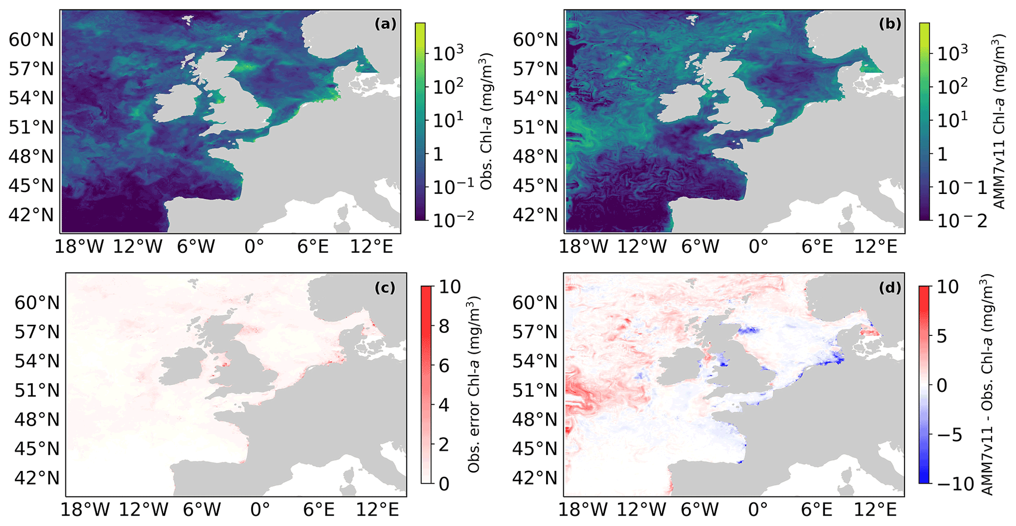
Figure 1(a) Daily mean L4 multi-sensor observations regridded on the 7 km resolution model grid and (c) AMM7v11 Chl a for 1 June 2019. (c) Error estimates on the multi-sensor L4 Chl a and (d) difference between AMM7v11 and the L4 product.
Figure 1 shows the L4 ocean colour product (a) and AMM7v11 analysis (b) for 1 June 2019 on the top row, using the same plotting ranges. The second row shows the difference field that is provided with the L4 ocean colour product (c), and the AMM7v11 minus L4 difference field (d). The mean error (bias) is generally positive with the AMM7v11 analysis containing higher Chl-a concentrations, especially in the deeper North Atlantic waters. The exceptions are along the coast where the AMM7v11 analysis is deficient, but it should be noted that these are also the zones where some of the largest satellite retrieval errors occur and where a 7 km resolution model, with a coarse representation of the coast, does not fully represent complex coastal and estuarine processes.
3.1 Description of the methods
This section provides a brief description of MODE, first described in Davis et al. (2006), and its time extension MTD.
MODE and MTD can be used on any temporal sequence of two gridded data sets which contain features that are of interest to a user (whoever that user may be, model developer or more applied). By extracting only the feature(s) of interest, the method allows one to mimic what humans do, but in an objective way. Once identified the features can then be mathematically analysed over many days or seasons to compute aggregate statistics of behaviour. MODE can be used in a very generalised way. The key requirements are to (1) have gridded fields to compare and (2) be able to set a threshold for identifying features of interest.
In this instance, the comparison will involve the AMM7v11 model data assimilation analysis and the gridded L4 satellite product. MODE identifies the features (called objects), as areas for which a specified threshold is exceeded; here, it is a Chl-a concentration. Consider Fig. 2, which shows a number of objects that have been identified after a threshold has been applied to two fields (blue and orange). The identified objects in the two fields are of different sizes and shapes and do not overlap in space, though they are not far apart. Object characteristics or attributes such as the area and mass-weighted centroid are computed for each single object. Simple (also known as single) objects can be “merged” (to form clusters) within one field (illustrated here for the orange field). This may be useful to do if it is clear that there are many small objects close together which should really be treated as one. Furthermore, objects in one field can be “matched” to objects in the other field. To find the best match, an interest score is computed for each possible pairing between all identified objects. The components used for computing the interest score can be tuned to meet specific user needs. In Fig. 2a, it is based on the area ratio, intersection–area ratio, minimum boundary distance and centroid difference. Furthermore, the components can be weighted according to relative importance. Given a scenario where there are two identified objects in the blue field and three in the orange field, Fig. 2b shows the interest score for each possible pairing in this hypothetical example. Only the pairing with the highest score is analysed further, and only if it exceeds the set threshold for defining an acceptable match. The default value for this is 0.7. In the example in Fig. 2b, blue object 1 is best matched against orange object 1, and this match is used in the analysis. Note that there is another good match with orange object 2, as it is above the threshold of 0.7, but it, as well as orange object 3, would not be used, with orange object 3 below the 0.7 threshold. In all likelihood, a scenario such as that shown in Fig. 2b would be assessed as clusters with blue objects 1 and 2 forming a cluster and orange objects 1 and 2 also forming a cluster. An interest score for the cluster pairing above 0.7 would then create a matched pair. Once these matches are completed, summary statistics describing the individual objects (both matched and unmatched) and matched object pairs are produced. These statistics can be used to identify similarities and differences between the objects identified in two different data sets, which can provide diagnostic insights on the relative strengths and weaknesses of one compared to the other.
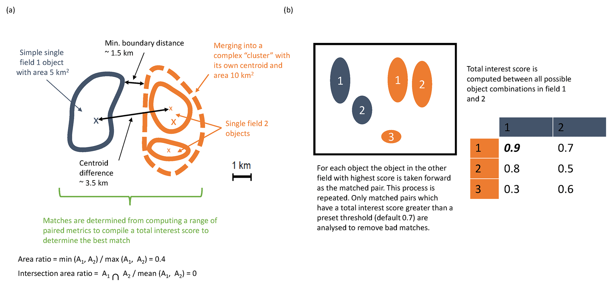
Figure 2Schematic illustrating some of the key components of identifying objects using MODE. (a) Defining some of the terminology and key components for computing matched pairs. (b) Example of how the best matched pair is identified.
The important steps for applying MODE can be summarised as follows (which are described in detail in Davis et al., 2006):
-
Both forecast and observation (or analysis) need to be on the same grid. Typically, this means interpolating the observations to the model grid to avoid the model being expected to resolve features which are sub-grid scale.
-
Depending on how noisy the fields are, they should be smoothed. Gridded observations (not analyses) can be noisy and usually need some smoothing. Models and model analyses are built on numerical methods which come with discretisation effects. Depending on the method this implies that any model's true resolution (i.e. the scales which the model is resolving) is between 2 and 4 times the horizontal grid (mesh) resolution. The number of objects identified will vary inversely with the smoothing radius.
-
Define a threshold which captures the feature of interest and apply it to both the smoothed forecast and observed fields to identify simple objects as shown in Fig. 2.
-
Any smoothing is only for object identification purposes. The original intensity information within the object boundaries is analysed.
-
Lastly, the object matching is accomplished using a fuzzy logic engine (low-level artificial intelligence), which is expressed as the so-called “interest” score as shown in Fig. 2b. The higher the score, the stronger the match. All objects are compared in both fields and interest scores are computed for all combinations. A threshold is set on the interest score value (typically 0.7) to denote which are the best matches, and on the unique pairing with the highest score is kept for analysis purposes. Some objects will remain unmatched (either because there are none or because there are no interest values above the set threshold to provide a credible match), and these can be analysed separately.
MODE is highly configurable. Gaining an optimal combination of configurable parameters for each application requires extensive sensitivity testing to gain sufficient understanding of the behaviour of the data sets to be examined and to achieve, on average, heuristically the right outcome. Initial tuning requires user input to check whether the method is replicating what a human would do.
The sensitivity to threshold and smoothing radius should be explored. The threshold and variability in the fields can affect the number of objects which are identified. The process of exploring the relationship between threshold and smoothness helps to identify what would heuristically be considered a reasonable number of objects.
The sensitivity to the merging option must also be investigated. In this instance, the merging option had very little impact.
The behaviour of the matching can also be configured, with a number of options ranging from the simple to the more complicated, which added computational expense. There may be very little difference in outcomes, but it is worth checking. Here the merge_both option was used but it was not strictly necessary as there was little difference between the available options.
Note also that a minimum size (area) is set for object identification. This is often a somewhat pragmatic choice. If the size is set too small, too many objects are identified, which end up being merged. If it is too large, very few objects are identified. Here, a minimum area of 10 grid squares (∼70 km2) was used for an object to be included in the analysis. For this study, the default settings were used for matching and computing the interest score (as provided in the default configuration file; see example configuration files at https://github.com/dtcenter/MET/tree/main_v8.1/met/scripts/config, last access: November 2018). The default threshold of 0.7 for the interest score was also used to identify acceptable matches.
Identical to MODE, identifying time–space objects in MTD uses smoothing and thresholding. Applying a threshold yields a binary field where grid points exceeding the defined threshold are set to 1. At this stage, each region of non-zero grid points in space and time is considered a separate object, and the grid points within each object are assigned a unique object identifier. For MTD, the search for contiguous grid points not only means examining adjacent grid points in space but also the grid points in the same or similar locations at adjacent times to define a space–time object. The same fuzzy logic-based algorithms used for merging and matching in MODE apply to MTD as well. Similarly to MODE, a minimum volume must be set. Here, a volume threshold of 1000 grid squares (a summation of the daily object areas identified to be part of the space–time object) was imposed for space–time object identification to be included in the analysis. This represents the accumulated number of grid squares associated with an object over consecutive time slices. Otherwise, the default settings were used for object matching. For MTD, a lower interest score of 0.5 was used for matching objects. Finally, it is worth noting that the MODE and MTD tools, though similar, are completely independent of each other and were set up differently here. MODE is ideal for understanding the identified features in individual daily fields in some detail. MTD, it was felt, would be best used to look at larger scales. Here it was set up to capture the most significant (in size) and long-lasting blooms.
3.2 Defining Chl-a concentration thresholds and other choices on tuneable parameters
Chl a can vary over several orders of magnitude. Often log10 thresholds are used to match the fact that Chl a follows a lognormal distribution (e.g. Campbell, 1995). Defining thresholds can be difficult: on the one hand, there is the desire to only capture events of interest, so the thresholds should not be too low; on the other hand, if the thresholds are too high, no events are captured and there is nothing to analyse. From a regional (NW European Shelf) perspective, the values of interest are typically in the range of 3–5 mg m−3 (Schalles, 2006), though higher Chl-a concentrations can be measured in situ or diagnosed in satellite products. For this study, the data sets were not log transformed but thresholds were selected in such a way that they would correspond to being equally spaced in logarithmic space (where the Chl-a concentrations are approximately Gaussian), better reflecting the skewed underlying distribution shape of Chl-a concentrations. Three thresholds analysed: 2.5, 4 and 6.3 mg m−3. Here, the primary focus is on the results for the 2.5 mg m−3 threshold, though some results for the 4 and 6.3 mg m−3 thresholds are also presented.
In addition to the interpolation of the L4 ocean colour product onto the ∼7 km AMM7v11 grid, it is important to ensure that MODE and MTD use optimal settings for the fields under study. Results are sensitive to characteristics of the fields (how smooth or noisy). Right at the start, the emphasis was on finding the right combination of Chl-a concentration threshold and smoothing, balancing the need for identifying objects with keeping the number of objects manageable. The guiding principles in identifying the right combination were to ensure that the daily object count remained low enough, recalling that these methods were developed to mimic what a human would do. The human brain would struggle to cope with as many as 30, but this was considered to be an acceptable upper limit after considerable visual inspection of output. Furthermore, the smoothing applied needs to be reduced with increasing concentration thresholds because objects become smaller and are less frequent. This is to ensure that too much smoothing does not remove more intense objects from the analysis. However, pushing the concentration threshold too high may also be detrimental; depending on the input fields, identified objects may be spurious (due to, for example, a failure of quality control processes removing such). Too few objects also make the compilation of robust aggregated statistics impossible.
For the lower thresholds, 2.5 and 4.0 mg m−3, a smoothing radius of five grid squares (∼35 km) was applied to both L4 and AMM7v11 fields, but for highest threshold (here 6.3 mg m−3) the smoothing radius was reduced to three grid squares, to prevent the higher peak concentrations, which are often small in spatial extent, from being lost due to the smoothing. Tests of thresholds above 6.3 mg m−3 yielded too few objects to be analysed with any rigour. The smoothing was particularly necessary for the L4 product, which, because of its native 1 km resolution, is able to resolve very small (noisy) objects typically found near the coast and which a 7 km resolution model cannot resolve. For the MTD analysis, objects in the L4 ocean colour product and the AMM7v11 analyses were only defined using a Chl-a concentration threshold of 2.5 mg m−3.
4.1 Traditional statistics
Traditional verification metrics are based on a set of observations and a set of model outputs matched in time and space. The statistics that are typically considered (McEwan et al., 2021) are the median error (bias), median absolute difference (MAD) and Spearman rank correlation coefficient. The median bias gives indication of consistent differences between the model and observations, with a positive bias indicating the model concentration is higher than observed. The MAD provides an absolute magnitude of the difference. The Spearman rank correlation coefficient is the Pearson correlation coefficient between the ranked values of the model and observation data, so that if the model data increase when the observations do, they are positively correlated. It has the same interpretation as the more common Pearson correlation coefficient where a correlation of 1 shows perfect correlation and 0 shows no correlation. Figure 3 provides a map of the model domain and the subregions over which traditional metrics are computed. Table 1 shows results for log(Chl a) assessed against the L4 ocean colour product.
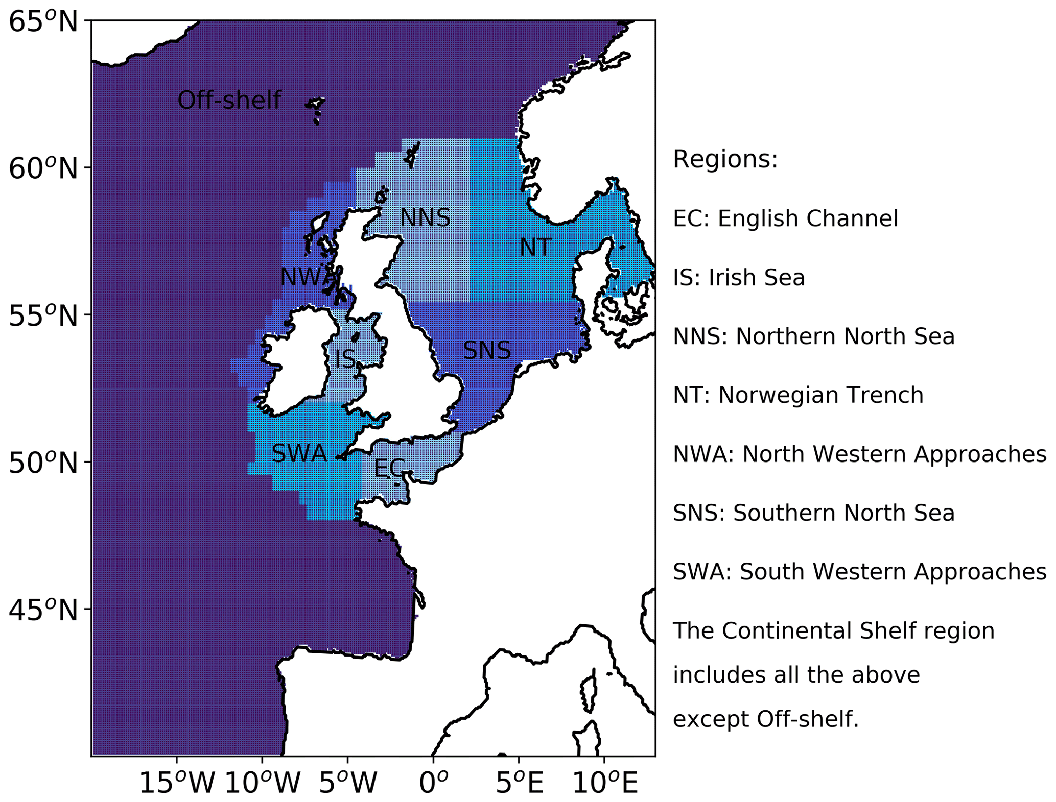
Figure 3Map showing the subregions over which statistics are computed.
Table 1Statistics for daily model surface log(Chl a) outputs and satellite ocean colour Chl a for the full domain and subregions for the period March to July 2019. See Fig. 3 for the location of the regions. The Continental Shelf includes all regions except those that are off-shelf (reproduced from McEwan et al., 2021).
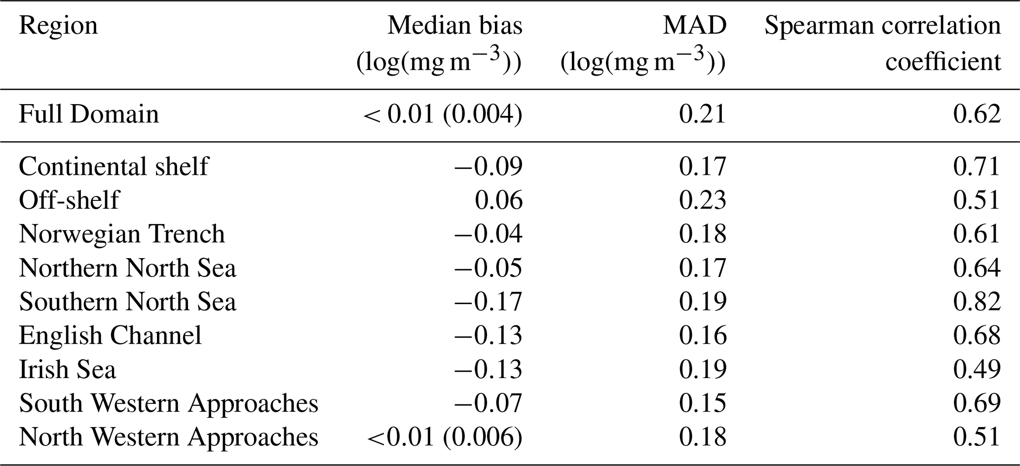
Compared with the L4 product, the AMM7v11 analysis slightly overestimates Chl a off-shelf and underestimates Chl a in the on-shelf regions (Table 1). Regions show moderate to strong positive correlations, highest in the Southern North Sea and lowest in the Irish Sea. These statistics give useful insight into model skill but provide limited information about how model performance changes as the bloom season progresses (McEwan et al., 2021; Skákala et al., 2018, 2020). As will be shown, the output from MODE and MTD provides a very different perspective from these traditional verification metrics, allowing a more detailed understanding of model performance.
4.2 Chl-a distributions
It is important to understand the nature of the underlying L4 and AMM7v11 Chl-a distributions and any differences between them. This can be done by creating cumulative distribution functions (CDFs) of the log10 L4 and AMM7v11 Chl-a concentrations, by taking all grid points in the domain and all dates in the study period. These are plotted in Fig. 4, showing that there is an offset between the distributions, the AMM7v11 analysis having more low concentrations, though the distributions appear to be converging in the upper tail.
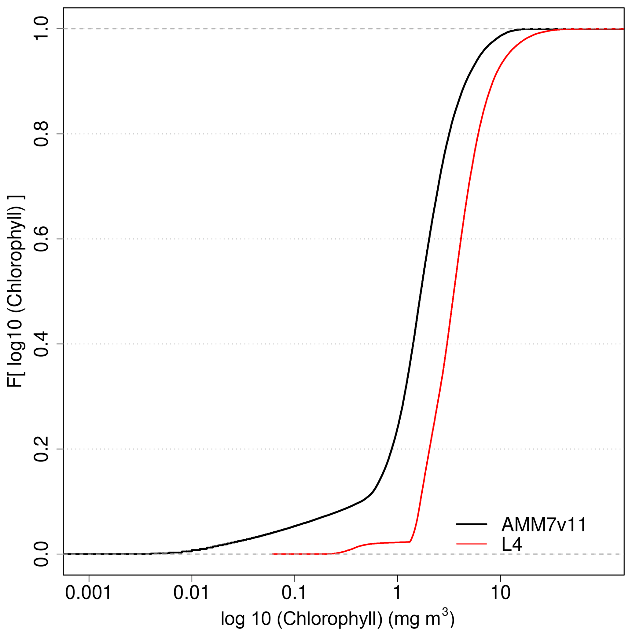
Figure 4Empirical cumulative distribution functions of the log10 Chl-a concentration for the L4 ocean colour product and AMM7v11 analyses for the 2019 bloom season.
Exploring this further, the AMM7v11 and L4 Chl-a concentration CDFs can be derived for each individual day, rather than for the season as a whole. From these, the quantile where the L4 product is less than or equal to 2.5 mg m−3 (29.7 %) can be compared to the corresponding AMM7v11 concentration associated with the same quantile of 29.7 %. From Fig. 4, this gives an equivalent concentration of 1.15 mg m−3 for the season. The daily matched quantile Chl-a values provide an estimate of the daily bias. This is plotted in Fig. 5 as a time series for the 2019 bloom season. It shows that the daily AMM7v11 corresponding quantile values are mainly in the range of ∼1.5–4.5 mg m−3, averaging out to 2.9 mg m−3 over the season, which suggests a modest difference overall. The larger day-to-day variations show some cyclical patterns. There are notable peaks at the end of May and the beginning of July. An inspection of the fields (not shown) suggests that at these times the AMM7v11 appears to have higher Chl-a concentrations over large portions of the domain compared to the L4 product.
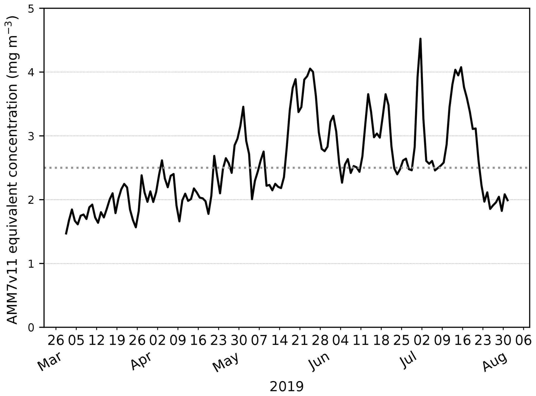
Figure 5The day-to-day AMM7v11 quantile Chl-a value corresponding to the L4 product quantile representing 2.5 mg m−3 derived from the L4 daily CDFs. The mean AMM7v11 Chl-a equivalent quantile value for the 2019 season is 2.9 mg m−3.
In employing a threshold-based approach, generally the same threshold is applied to both data sets. In the presence of a bias, this requires a little bit of thought. In extreme cases, it could mean the inability to identify objects in one of the data sets, which would then mean objects cannot be matched and paired, negating the purpose of a spatial method like MODE or MTD. Not being able to identify any objects does provide some useful information, though arguably not enough context. The lack of objects does suggest the presence of a bias, but it does not provide any sense of whether the model is producing a constant value of Chl a, for example, which would be of no use to the user, or whether it does capture regions of enhanced Chl a, albeit with an offset which means it does not exceed the set threshold. Therefore, a more likely scenario is that a bias could partially mask relevant signals in the derived object properties, which could lead to the potential misinterpretation of results. If there is a significant risk of this occurring the bias could be addressed before features are identified to ensure that the primary purpose of using a feature-based assessment can be achieved, i.e. identifying features of interest in two sets of fields to assess their location, timing and other properties and assessing their skill. The fact that there is an intensity offset should not prevent the method from providing information about the skill of identified features. As is seen here, though there is bias (as seen in Figs. 4 and 5), it does not prevent the method from successfully identifying objects using the same threshold for both data sets, though it will be shown that the effect of the bias can affect some object attributes, e.g. object areas. However, a more prohibitive bias could compromise the methods, e.g. being unable to identify objects in a data set. This would have a disproportionate effect on the statistics for the matched pairs in particular. Under such circumstances, the quantile-mapping functionality within MODE (to remove the effect of the bias) is strongly recommended.
4.3 Visualising daily objects
Figure 6 shows the daily Chl-a concentration fields as represented in the L4 ocean colour product and the AMM7v11 analyses for 21 April 2019, which is near the peak of the bloom season. The respective fields are plotted in (a) and (b), noting that the 1 km resolution L4 product has been interpolated onto the ∼7 km AMM7 grid. Applying a threshold of 6.3 mg m−3 to both with a smoothing radius of ∼21 km (three grid lengths) yields eight objects in the AMM7v11 analysis (seven visible in this zoomed region) and 11 objects in the L4 product. As discussed, the bias described in Sect. 4.1 does not appear to prevent the identification of objects in the L4 product and the AMM7v11 analyses, and the process of finding matches is possible.
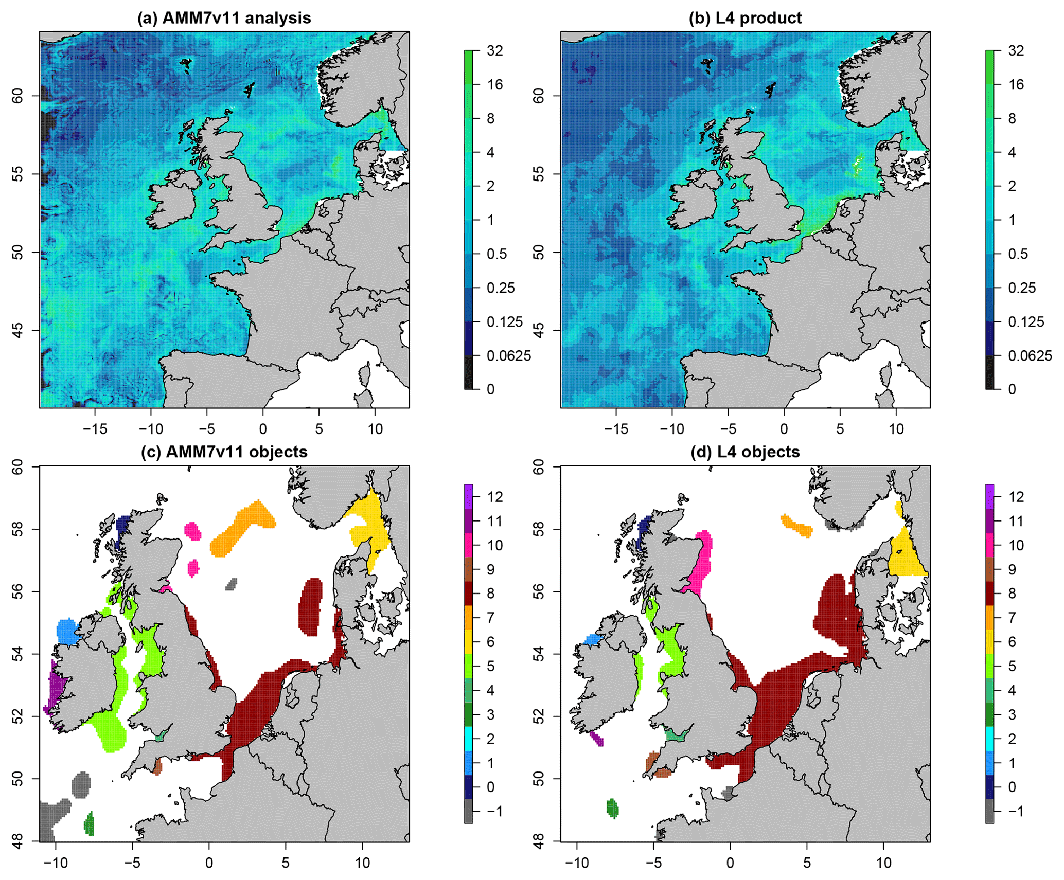
Figure 6Daily Chl-a concentrations (in mg m−3 for 21 April 2019: (a) AMM7v11 analysis and (b) L4 ocean colour product. The MODE objects shown in panels (c) and (d) are identified using a threshold of 6.3 mg m−3 and a smoothing radius of ∼ 21 km. Note that panels (c) and (d) show a smaller (inner) domain. The colours show the matching clusters. Objects denoted with −1 (grey) are unmatched.
4.4 Spatial characteristics
This section demonstrates the kinds of results that can be extracted from the two-dimensional MODE objects. Aspects of the marginal (AMM7v11 or L4 product only) and joint (matched/paired) distributions can be examined. This includes object size (as a proxy for area) but also the proportion of areas that are matched or unmatched.
Firstly, how similar is the L4 ocean colour product and the AMM7v11 analysis in terms of the features of most interest, i.e. the Chl-a blooms? Figure 7 shows the evolution of the proportion of matched object areas (to total combined area) through the 2019 season, when using MODE to compare the L4 product and AMM7v11 analyses, to further explore the differences (and similarities) between them. A value of 1 would indicate that all identified areas are matched. Values less than 1 suggest that some objects remain unmatched. The relatively high values of matched object to total area during April are due to the large numbers of well-matched, physically small coastal objects in addition to the larger Chl-a bloom originating in the Dover Straits (not shown). There is a notable minimum at the beginning of July. Inspecting the MODE graphical output reveals this is in part due to only a few small objects being identified, and this is compounded by their complete mismatch; the L4 objects are all coastal, whilst the AMM7v11 objects are either coastal (but not in the same location as L4 objects) or in the deep waters of the North Atlantic, to the northwest of Scotland. The relatively high proportions on either side of this time arise from a better correspondence in placement of the coastal objects (noting that there is a distance limit on how far objects can be apart for the matching process to have a positive contribution to the interest score).
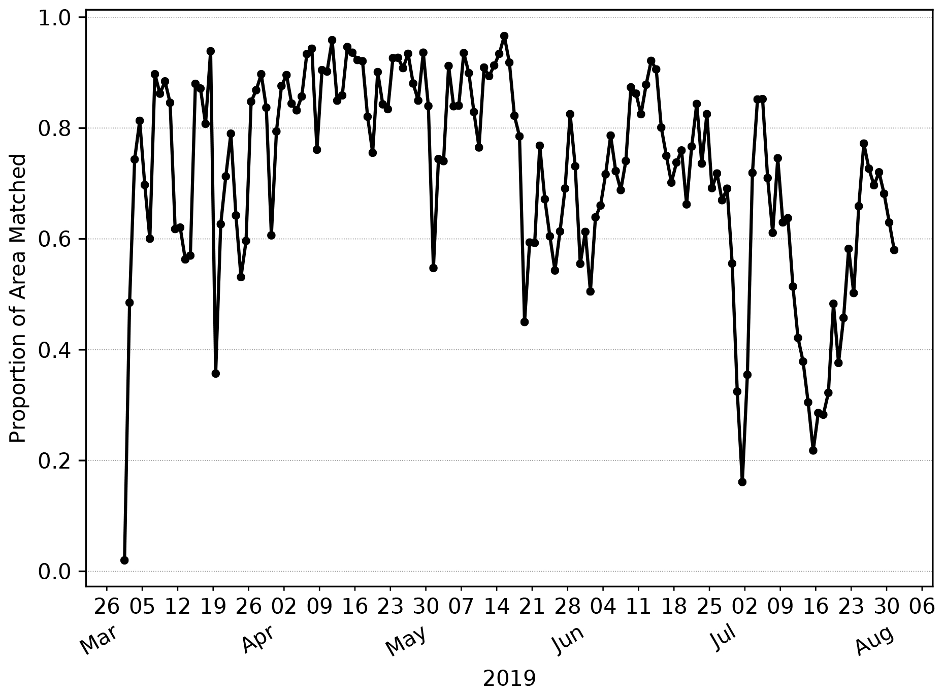
Figure 7Proportion of total object area which is matched. Underlying matched and unmatched object areas (in units of numbers of grid squares) are taken from the MODE output. These areas are for the 2.5 mg m−3 concentration threshold objects.
Overall, the AMM7v11 analysis is similar, but clearly not identical, to the L4 product. The best correspondence appears to be during the first half of the bloom season. Later in the season, the model's determination to produce blooms in deep North Atlantic waters is a model deficiency that the assimilation is (at this stage) unable to fix. The AMM7v11 analyses could conceivably be used as a credible source for assessing the AMM7 Chl-a forecasts in the future. The major benefit of using a model analysis is that it is at the same spatial resolution, with the same ability to resolve Chl-a bloom objects, especially along the coast (i.e. the analysis limits the uncertainty due to whether an object could be missing due to the inability of the model to resolve the feature).
The day-to-day number of objects identified through the 2019 bloom season is shown in Fig. 8, illustrating how elements of the marginal and joint distribution provided by MODE can be used together. Here, numbers of total and matched (joint) objects are shown. If the AMM7v11 analyses are good (i.e. similar to the L4 product), there should be fewer unmatched (marginal) objects than matched ones (indicated by the proximity of the solid and dashed lines); ideally, there would be no unmatched objects in either the L4 product or the AMM7v11 analysis. In Fig. 8, the number of objects in AMM7v11 starts off small and increases as the bloom develops. For the L4 product, there are already many objects identified at the start of the time series, leading to many unmatched L4 objects (these could be considered misses in a more categorical analysis). A spike in the number of matched objects seen in early April can be attributed to several coastal locations, which appear to be spatially well matched. In addition, a larger Chl-a bloom is seen in the Dover Straits region in the L4 product and although not exactly spatially collocated, the objects are matched. There is a consistently large number of unmatched objects seen in the AMM7v11 analysis and L4 ocean colour product from the end of May onwards. In the AMM7v11 analysis, this appears to be due to an increase in small objects identified, mainly to the west, north and east of the United Kingdom. The increase in unmatched objects in the L4 ocean colour product is of a different origin, being due to an increase in localised coastal blooms. Generally, the AMM7v11 analyses do not have the resolution to resolve these. Overall, there are 2632 AMM7v11 bloom objects identified in the season using the 2.5 mg m−3 threshold, and 2341 L4 bloom objects, with 56 % of AMM7v11 objects matched and 59 % of L4 objects matched.
The identified objects in AMM7v11 and the L4 product can also be considered spatially over the season by compositing the objects. This is done by counting the frequency with which a given grid square falls within an identified object on any given day, essentially creating a binary map. These can be added up over the entire season to produce a spatial composite object or temporal “frequency-of-occurrence” plot.
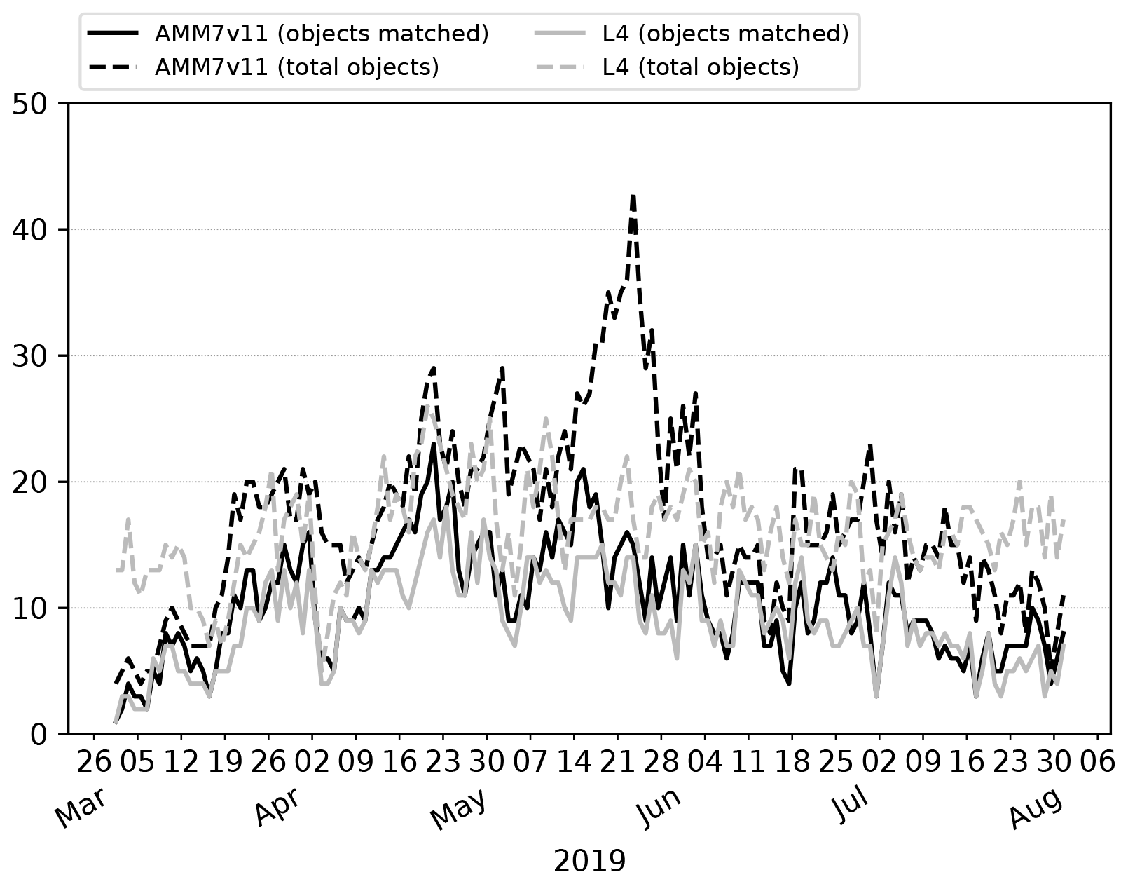
Figure 8Time series of the number of matched and total objects per day from MODE comparing AMM7v11 analyses (black) with L4 satellite product (grey). Objects are identified using a threshold of 2.5 mg m−3. Total object numbers for the season are 2341 for the L4 satellite product and 2632 for AMM7v11.
Figure 9 shows this spatial composite for the 2019 bloom season for the L4 ocean colour product objects (a) and the AMM7v11 objects (b). These are the composites based on the 2.5 mg m−3 threshold objects. There are areas, for example, in the South Western Approaches (SWAs; see Fig. 3), where there appears to be a good level of consistency. AMM7v11 analyses have elevated Chl-a values along the northern and western edges of the domain, for a low proportion of the time, which are not seen in the L4 product. This is likely due to the way that nutrient and phytoplankton boundary conditions are specified in AMM7v11. Overall, the low temporal frequency extent of the AMM7v11 objects is greater than that for the L4 product.
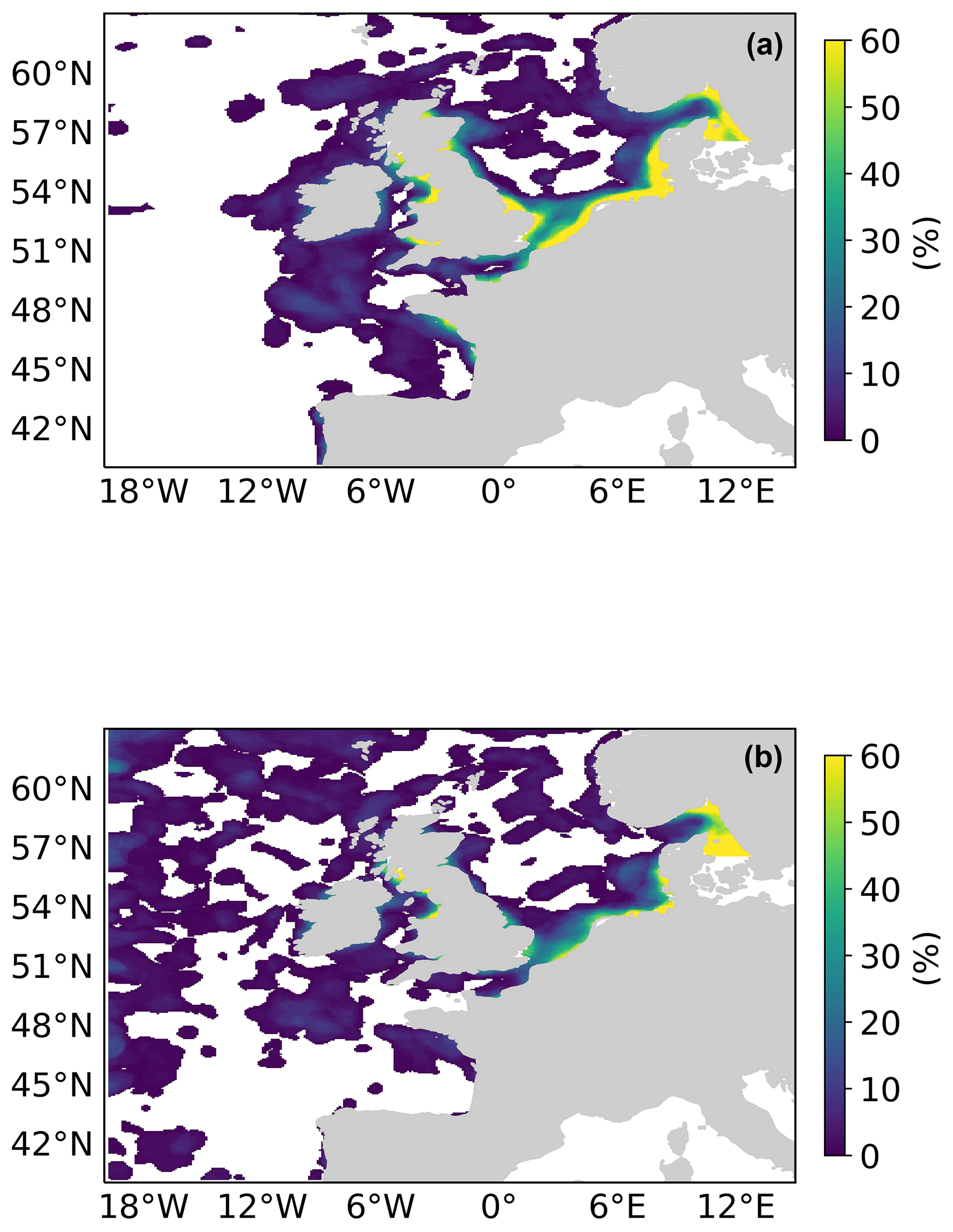
Figure 9Object composites (the proportion of time for which an object was present at the grid box throughout the 2019 bloom season) for (a) the L4 ocean colour product objects and (b) the AMM7v11 analysis objects.
Thus far, all the attributes have been based on only the AMM7v11 or L4 objects. The distribution of object properties, derived for the season from the daily comparisons, can be summarised using box-and-whisker plots. Recall that the box encompasses the interquartile range (IQR, 25th to 75th quantiles) and the notch and line through the box denotes the median or 50th quantile. The dashed line represents the mean, and the whiskers show ±1.5 times the IQR. For clarity, values outside that range have been filtered out of the plots shown here. Figure 10 shows the intersection-over-area paired object attribute distribution as box-and-whisker plots for all object pairs during the 2019 bloom season, comparing the AMM7v11 analyses to L4 for three of the thresholds: 2.5 and 4.0 and 6.3 mg m−3. The intersection-over-area diagnostic gives a measure of how much the matched (paired) objects overlap in space. If the objects do not intersect, this metric is 0. The ratio is bounded at 1 because any area of overlap is always divided by the larger of the two object areas. The IQR for the 2.5 mg m−3 threshold is 0.25 with 50 % of paired objects having an intersection-over-area ratio of 0.97 or greater. However, the lower whisker spans a large range of values to as low as 0.375, suggesting that there is a proportion of object pairs with only small overlaps. There is quite a difference between the median (notch) and the mean (dashed line) for this metric, suggesting the distribution is skewed with the mean affected more by many small overlaps. For the 4.0 mg m−3 threshold paired objects, the intersection-over-area distribution is much broader, though the difference between the mean and medians is similar. The proportion of paired objects with smaller overlaps has also increased. This should not be surprising given that the objects generally get smaller with increasing threshold such that the ability for object pairs to overlap actually decreases unless they are very closely collocated. At the 6.3 mg m−3 threshold, the median is lower (0.93) with a similar difference from the mean; however, the sample size is much smaller (only 130 paired objects over the season).
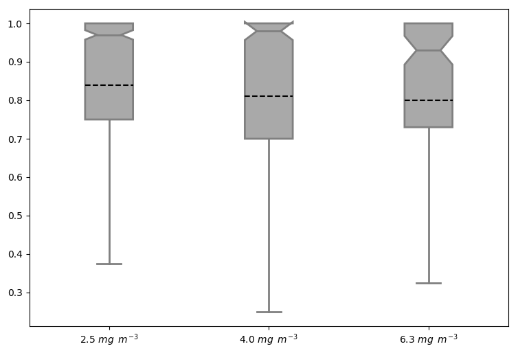
Figure 10Box-and-whisker plots of the paired object property intersection-over-area ]ratio computed by dividing the spatially collocated area between the paired objects by the largest of either the AMM7v11 or L4 observed object areas (to keep the ratio to be bounded by 0 and 1). Three object thresholds are shown: 2.5, 4.0 and 6.3 mg m−3. Smoothing radii of 5, 5 and 3 grid lengths were applied for the three thresholds, respectively. The sample sizes for each threshold were 1004, 401 and 130 paired objects, respectively.
4.5 Incorporating the time dimension
Having information in space and time enables one to ask, and hopefully answer, questions such as “did the model predict the bloom to start in the observed location?” or “did the model predict the onset at the right time?” and “did the model predict the peak (in terms of extent) and duration of the bloom correctly?”.
MTD identifies objects in space and time. As previously described, all MTD results are based on a 2.5 mg m−3 threshold applied to both the L4 ocean colour products and AMM7v11 analyses. A time centroid is derived from a time series of the spatial (two-dimensional) centroids which are computed for each (daily) time slice. In addition to this, each identified MTD object has a start and end time, and a geographical location of the time centroid, which is the average of the two-dimensional locations. The time component of the time centroid is weighted by volume.
The temporal progression of the 2019 bloom season along with spatial information as defined by the MTD objects' is shown in Fig. 11. The object start and end times as well as the date of their time centroids in (a) provide a clear view of the onset and demise of each object (bloom episode). In total, there are 22 AMM7v11 and 11 L4 MTD objects. The x axis in (a) represents elapsed time. The location of the vertical lines along the x axis on any given date indicates the date of the time centroid whilst the duration of the space–time object can be gleaned from the y axis based on the start and end of the vertical line which defines the time the object was in existence. Solid lines represent the L4 product objects whereas dashed lines represent the AMM7v11 objects. The colour palette is graduated from grey and blue through green, yellow, red and purple, denoting the relative time in the season. In (a), the first Chl-a bloom object in the AMM7v11 analysis was identified on 29 March 2019, whereas in the L4 ocean colour product the first bloom object was identified on 3 March, 26 d earlier. The first time the L4 product and AMM7v11 analyses have concurrent objects (blooms) is in late March. The L4 product also suggests that the season ends 30 June, whereas in the AMM7v11 analyses the bloom season persists with objects identified until 23 July. Most AMM7v11 objects are of relatively short duration, but overall, most groups of AMM7v11 objects have some temporal association with an L4 product object around the same time. In this instance, it is also illuminating to consider the daily object areas associated with the MTD objects (which are used to compute the volume of MTD objects). These are plotted in Fig. 11b showing all daily L4 object areas in the filled circles, and the AMM7v11 object areas (crosses), in the same colours as in (a). The main purpose is to highlight the relative size of the L4 and AMM7v11 objects on any given day, as well as how many objects there were. Recall that these are the objects identified using a Chl-a concentration threshold of 2.5 mg m−3. Some of the AMM7v11 objects are considerably larger than those in L4 in the middle and latter parts of the bloom season from mid-May onwards, just not necessarily at exactly the same time or location. As seen in Fig. 11b, the area time series also illustrates the offsets in the start and end of the bloom season. Some of the objects detected in AMM7v11 beyond the end of the observed bloom season provided by L4 suggest that at least three substantial areas are still diagnosed to exceed the threshold of 2.5 mg m−3 into July. Taking the start of the earliest space–time object as the onset of the bloom season and the end of the last object as the end, the 2019 season is 119 d long based on the L4 product, and 117 d in the AMM7v11 analysis. Therefore, the overall length of the season as defined by the space–time objects is comparable in the AMM7v11 analysis, albeit with a substantial offset. Finally, even if (a) and (b) suggest that AMM7v11 and L4 objects exist at the nearly the same time, this does not mean they are geographically close to each other. This is illustrated in Fig. 11c, which provides the spatial context. The colours and symbols are consistent across all panels and show that even when the MTD objects are identified at the same time they may be geographically quite far apart, or more typically there is no L4 counterpart (filled circle) to an AMM7v11 bloom object (cross). The north- and westward progression of the bloom as the season unfolds can be seen through the use of the colours, with the AMM7v11 analysis producing enhanced Chl a concentrations in deeper waters to the north and west of the domain beyond the end of the observed season.

Figure 11Space–time information from the L4 (filled circle) and AMM7v11 (cross) MTD objects. (a) The timing of each identified bloom event (time centroid) plotted on the x axis against the duration of the bloom event, denoted by the vertical line which represents the start and end time of each space–time object. (b) Daily object areas. (c) Spatial location of the time centroid shown in panel (a) to indicate that even if AMM7v11 and L4 objects exist at the same time, they may not be geographically close. Colours are coordinated across all panels.
With only 22 AMM7v11 and 11 L4 product MTD objects, which are temporally and geographically well dispersed, three of the L4 objects remained unmatched, leaving only eight matched MTD objects for the 2019 bloom season with an overall interest score greater than 0.5. This represented an insufficient sample for drawing any robust statistical conclusions. Nevertheless, some inspection of the paired MTD object attributes is summarised below:
-
The spatial centroid (centre of mass) differences can be extensive, but the majority are within 0 to 100 grid squares apart (i.e. up to ∼ 700 km).
-
The majority of paired objects have time centroid differences ± 10 d.
-
Considering the volumes of the space–time objects, half the paired objects have volume ratios of less than 1; i.e. AMM7v11 objects tend to be smaller or similar in size. The other pairs have ratios as high as 4.
-
Overlaps between AMM7v11 and L4 MTD objects remain small and infrequent with only one pair with a significant overlap in space and time.
The traditional statistics provided in Table 1 give useful insights into overall performance, but even when the full domain is divided into subregions, they do not focus on the events of interest enough to provide more detailed information on the evolution of bloom events as the season progresses.
MODE and MTD, two distinct but related feature-based diagnostic verification methods, provide more detailed diagnostic information in space and time. This was demonstrated by using these two methods to evaluate and compare the pre-operational AMM7v11 European Northwest Shelf Chl a concentration bloom objects to those identified in the satellite-based L4 ocean colour product. Nominally, blooms were said to occur when the concentration threshold exceeded 2.5 mg m−3, and two higher thresholds were also considered. Sample sizes dwindle rapidly with increasing threshold. Of specific interest were the similarities and differences in respective bloom object sizes, their geographical location and collocation and timing. For the timing component the onset, duration and demise of individual bloom objects (events) could be considered. For the season, all the identified space–time objects provided an estimate of the onset, duration and end of the bloom season as a whole. The season was found to be of similar length, but the onset was found to begin 26 d later in the AMM7v11 analyses than in the L4 product, and the AMM7v11 analyses persist the season for almost a month beyond the diagnosed end identified in the L4 product. Using traditional verification methods, data assimilation has been shown to considerably reduce the delay in bloom onset in the model (Skákala et al., 2020). Using feature-based verification methods, this study suggests that a substantial delay still remains.
There is a modest concentration bias in the AMM7v11 analyses compared to the L4 satellite ocean colour product. In this study, we chose not to mitigate against this bias as it was not considered to impede the identification of bloom objects, which would prevent the ability of the methodology to identify matches and create paired object statistics. Any concentration bias does affect the results and this effect must be understood or at least kept in mind when interpreting results; in this case, it will have contributed to the result that the AMM7v11 bloom objects are generally larger. An alternative approach would be to mitigate against the impact of the bias before using a threshold-based methodology such as MODE or MTD. A quantile-mapping approach is available within the MODE tool (not yet available in MTD but should be available at some point) to remove the biases between two distributions as each temporal data set is analysed. Using this method, the one threshold is fixed, and the other threshold varies day to day (as shown in Fig. 5). Another approach would be to analyse the bias for the whole season (as shown in Fig. 4) and deriving an equivalent threshold from this larger data set, thus applying a fixed threshold to all the days in the season, though there would still be two different thresholds applied to the two data sets.
MODE results suggest that the AMM7v11 bloom objects are larger than those in the L4 product. AMM7v11 produces more objects (in number) than seen in the L4 ocean colour product, yet many of the coastal objects seen in the L4 product are not as well resolved in AMM7v11 due to the coarseness of the coastline in the 7 km model. The additional AMM7v11 objects are mainly found in deeper Atlantic waters. The diagnosis of coastal blooms should improve if the model resolution was increased from 7 to 1.5 km.
Using MODE and MTD clearly gives extra information not obtained from traditional verification metrics that are more routinely used (McEwan et al., 2021). An alternative approach to assessing the representation of phytoplankton blooms might be to use phenological indices (Siegel et al., 2002; Soppa, et al., 2016), which measure the day of the year on which Chl a concentration first crosses a threshold based on the median concentration. Phenological indices have been used in observation and model-based process studies (e.g. Racault et al., 2012; Pefanis, 2021), but rarely for model verification, and then usually in 1-D (Anugerahanti et al., 2018) or at low temporal resolution (Hague and Vichi, 2018). One reason for this is that daily model Chl a will frequently cross such a threshold throughout the bloom season, meaning temporal smoothing and other processing (Cole et al., 2012) would be required, which is not straightforward to apply consistently. Objective methods such as MODE and MTD, which consider individual bloom objects throughout the season, rather than assuming a single spring bloom will occur at each location, bypass these difficulties.
Other work that formed part of this study, but is not reported on here, showed that constraining the Chl a using assimilation of the satellite observations appears to benefit the model in terms of fewer unmatched bloom regions. This should translate to an improvement in the forecasts generated from this analysis compared with previous versions of the operational system and will be the subject of future work.
Model Evaluation Tools (MET) was initially developed at the National Center for Atmospheric Research (NCAR) through grants from the National Science Foundation (NSF), the National Oceanic and Atmospheric Administration (NOAA), the United States Air Force (USAF), and the United States Department of Energy (DOE). The tool is now open source and available for download from https://doi.org/10.5281/zenodo.5567805 (Win-Gildenmeister et al., 2021). Over the course of the project, MET versions 8 to 9.1 were used, with local versions updated when they became available. MET allows for a variety of input file formats, but some pre-processing of the CMEMS NetCDF files was necessary before the MODE package could be applied. This includes regridding of the observations onto the model grid and the addition of the forecast reference time variables to the NetCDF attributes. All aspects of the use of MET are provided in the MET software documentation available online.
Data used in this paper were downloaded from CMEMS.
-
The Chl a satellite observations used for comparison are provided by ACRI-ST Company (Sophia Antipolis, France) and distributed through CMEMS (https://resources.marine.copernicus.eu/product-detail/OCEANCOLOUR_ATL_CHL_L4_REP_OBSERVATIONS_009_098/INFORMATION, last access: 12 September 2021) (CMEMS, 2021a)
-
The model outputs are produced by the Met Office and distributed via CMEMS (https://resources.marine.copernicus.eu/product-detail/NWSHELF_ANALYSISFORECAST_BGC_004_002/INFORMATION, last access: 5 October 2021) (CMEMS, 2021b).
The AMM7v11 analyses were not operational at the time of this study, but part of the bloom season (from 4 May 2019) has become publicly available since the study.
All authors contributed to the introduction, data and methods, and conclusions. MM, RN, JM and CP contributed to the scientific evaluation and analysis of the results. MM and RN designed and ran the model assessments. CP supported the assessments through the provision and reformatting of the data used. DF provided details on the model configurations used.
The contact author has declared that neither they nor their co-authors have any competing interests.
Publisher's note: Copernicus Publications remains neutral with regard to jurisdictional claims in published maps and institutional affiliations.
This study has been conducted using EU Copernicus Marine Service information.
This work has been carried out as part of the Copernicus Marine Environment Monitoring Service (CMEMS) HiVE project. CMEMS is implemented by Mercator Ocean International in the framework of a delegation agreement with the European Union.
We would like to thank the National Center for Atmospheric Research (NCAR) Developmental Testbed Center (DTC) for the help received via their met_help facility in getting MET to work with ocean data and Robert McEwan (Met Office) for his assistance with the production of the traditional metrics.
This paper was edited by Andrew Moore and reviewed by two anonymous referees.
Allen, J. I. and Somerfield, P. J.: A multivariate approach to model skill assessment, J. Mar. Syst., 76, 83-94. https://doi.org/10.1016/j.jmarsys.2008.05.009, 2009.
Allen, J. I., Holt, J. T., Blackford, J., and Proctor, R.: Error quantification of a high-resolution coupled hydrodynamic-ecosystem coastal-ocean model: Part 2. Chlorophyll-a, nutrients and SPM, J. Mar. Syst., 68, 381-404, https://doi.org/10.1016/j.jmarsys.2007.01.005, 2007a.
Allen, J. I., Somerfield, P. J., and Gilbert, F. J.: Quantifying uncertainty in high-resolution coupled hydrodynamic-ecosystem models, J. Mar. Syst., 64, 3-14, https://doi.org/10.1016/j.jmarsys.2006.02.010, 2007b.
Antoine, D., André, J. M., and Morel, A.: Oceanic primary production: 2. Estimation at global scale from satellite (Coastal Zone Color Scanner) chlorophyll, Global Biogeochem. Cy., 10, 57-69, https://doi.org/10.1029/95GB02832, 1996.
Anugerahanti, P., Roy, S., and Haines, K.: A perturbed biogeochemistry model ensemble evaluated against in situ and satellite observations, Biogeosciences, 15, 6685–6711, https://doi.org/10.5194/bg-15-6685-2018, 2018.
Behrenfeld, M. J., Boss, E., Siegel, D. A., and Shea, D. M.: Carbon-based ocean productivity and phytoplankton physiology from space, Global Biogeochem. Cy., 19, GB1006, https://doi.org/10.1029/2004GB002299, 2005.
Bruggeman, J. and Bolding, K.: A general framework for aquatic biogeochemical models, Environ. Model. Softw., 61, 249–265, https://doi.org/10.1016/j.envsoft.2014.04.002, 2014.
Butenschön, M., Clark, J., Aldridge, J. N., Allen, J. I., Artioli, Y., Blackford, J., Bruggeman, J., Cazenave, P., Ciavatta, S., Kay, S., Lessin, G., van Leeuwen, S., van der Molen, J., de Mora, L., Polimene, L., Sailley, S., Stephens, N., and Torres, R.: ERSEM 15.06: a generic model for marine biogeochemistry and the ecosystem dynamics of the lower trophic levels, Geosci. Model Dev., 9, 1293–1339, https://doi.org/10.5194/gmd-9-1293-2016, 2016.
Campbell, J. W.: The lognormal distribution as a model for bio‐optical variability in the sea, J. Geophys. Res.- Ocean., 100, 13237-13254, 1995.
Chelton, D. B., Schlax, M. G., and Samelson, R. M.: Global observations of nonlinear mesoscale eddies, Prog. Oceanogr., 91, 167–216, https://doi.org/10.1016/j.pocean.2011.01.002, 2011.
Chiswell, S. M.: Annual cycles and spring blooms in phytoplankton: Don't abandon Sverdrup completely, Mar. Ecol. Prog. Ser., 443, 39–50, https://doi.org/10.3354/meps09453, 2011.
Clark, A. J., Bullock, R. G., Jensen, T. L., Xue, M., and Kong, F.: Application of object-based time-domain diagnostics for tracking precipitation systems in convection-allowing models, Weather Forecast., 29, 517–542, https://doi.org/10.1175/WAF-D-13-00098.1, 2014.
CMEMS: North Atlantic Chlorophyll (Copernicus-GlobColour) from Satellite Observations: Daily Interpolated (Reprocessed from 1997), available at: https://resources.marine.copernicus.eu/product-detail/OCEANCOLOUR_ATL_CHL_L4_REP_OBSERVATIONS_009_098/INFORMATION, CMEMS [data set], last access: 15 October 2021a.
CMEMS: Atlantic – European North West Shelf – Ocean Biogeochemistry Analysis and Forecast, available at: https://resources.marine.copernicus.eu/product-detail/NWSHELF_ANALYSISFORECAST_BGC_004_002/INFORMATION, CMEMS [data set], last access: 15 October 2021b.
Cole, H., Henson, S., Martin, A., and Yool, A.: Mind the gap: The impact of missing data on the calculation of phytoplankton phenology metrics, J. Geophys. Res., 117, C08030, https://doi.org/10.1029/2012JC008249, 2012.
Crocker, R. L. and Mittermaier, M. P.: Exploratory use of a satellite cloud mask to verify NWP models, Meteorol. Appl., 20, 197–205, 2013.
Crocker, R., Maksymczuk, J., Mittermaier, M., Tonani, M., and Pequignet, C.: An approach to the verification of high-resolution ocean models using spatial methods, Ocean Sci., 16, 831–845, https://doi.org/10.5194/os-16-831-2020, 2020.
Davis, C., Brown, B., and Bullock, R.: Object-based verification of precipitation forecasts, Part I: Methods and application to mesoscale rain areas, Mon. Weather Rev., 134, 1772–1784, 2006.
de Mora, L., Butenschön, M., and Allen, J. I.: The assessment of a global marine ecosystem model on the basis of emergent properties and ecosystem function: a case study with ERSEM, Geosci. Model Dev., 9, 59–76, https://doi.org/10.5194/gmd-9-59-2016, 2016.
Dorninger, M., Gilleland, E., Casati, B., Mittermaier, M. P., Ebert, E. E., Brown, B. G., and Wilson, L. J.: The setup of the MesoVICT project, B. Am. Meteorol. Soc., 99, 1887-1906. DOI: https://doi.org/10.1175/BAMS-D-17-0164.1, 2018.
Dutkiewicz, S., Hickman, A. E., and Jahn, O.: Modelling ocean-colour-derived chlorophyll a, Biogeosciences, 15, 613–630, https://doi.org/10.5194/bg-15-613-2018, 2018.
Edwards, K. P., Barciela, R., and Butenschön, M.: Validation of the NEMO-ERSEM operational ecosystem model for the North West European Continental Shelf, Ocean Sci., 8, 983–1000, https://doi.org/10.5194/os-8-983-2012, 2012.
Falkowski, P. G., Barber, R. T., and Smetacek, V.: Biogeochemical controls and feedbacks on ocean primary production, Science, 281, 200–206, https://doi.org/10.1126/science.281.5374.200, 1998.
Ford, D. A., van der Molen, J., Hyder, K., Bacon, J., Barciela, R., Creach, V., McEwan, R., Ruardij, P., and Forster, R.: Observing and modelling phytoplankton community structure in the North Sea, Biogeosciences, 14, 1419–1444, https://doi.org/10.5194/bg-14-1419-2017, 2017.
Gilleland, E., Ahijevych, D., Brown, B., and Ebert, E.: Intercomparison of Spatial Forecast Verification Methods, Weather Forecast., 24, 1416–1430. https://doi.org/10.1175/2009WAF2222269.1, 2009.
Gilleland, E., Lindström, J., and Lindgren, F.: Analyzing the image warp forecast verification method on precipitation fields from the ICP, Weather Forecast., 25, 1249–1262, 2010.
Gordon, H. R., Clark, D. K., Brown, J. W., Brown, O. B., Evans, R. H., and Broenkow, W. W.: Phytoplankton pigment concentrations in the Middle Atlantic Bight: comparison of ship determinations and CZCS estimates, Appl. Opt., 22 20–36, https://doi.org/10.1364/ao.22.000020, 1983.
Hague, M. and Vichi, M.: A Link Between CMIP5 Phytoplankton Phenology and Sea Ice in the Atlantic Southern Ocean, Geophys. Res. Lett., 45, 6566–6575, https://doi.org/10.1029/2018GL078061, 2018.
Hausmann, U. and Czaja, A.: The observed signature of mesoscale eddies in sea surface temperature and the associated heat transport, Deep. Res. Part I Oceanogr. Res. Pap., 70, 60–72, https://doi.org/10.1016/j.dsr.2012.08.005, 2012.
Hipsey, M. R., Gal, G., Arhonditsis, G. B., Carey, C. C., Elliott, J. A., Frassl, M. A., Janse, J. H., de Mora, L., and Robson, B. J.: A system of metrics for the assessment and improvement of aquatic ecosystem models, Environ. Model. Softw., 128, 104697, https://doi.org/10.1016/j.envsoft.2020.104697, 2020.
Jolliff, J. K., Kindle, J. C., Shulman, I., Penta, B., Friedrichs, M. A. M., Helber, R., and Arnone, R. A.: Summary diagrams for coupled hydrodynamic-ecosystem model skill assessment, J. Mar. Sys., 76, 64–82, 2009.
King, R. R., While, J., Martin, M. J., Lea, D. J., Lemieux-Dudon, B., Waters, J., and O'Dea, E.: Improving the initialisation of the Met Office operational shelf-seas model, Ocean Model., 130, 1–14, https://doi.org/10.1016/j.ocemod.2018.07.004, 2018.
Le Traon, P. Y., Reppucci, A., Fanjul, E. A., Aouf, L., Behrens, A., Belmonte, M., Bentamy, A., Bertino, L., Brando, V. E., Kreiner, M. B., Benkiran, M., Carval, T., Ciliberti, S. A., Claustre, H., Clementi, E., Coppini, G., Cossarini, G., De Alfonso Alonso-Muñoyerro, M., Delamarche, A., Dibarboure, G., Dinessen, F., Drevillon, M., Drillet, Y., Faugere, Y., Fernández, V., Fleming, A., Garcia-Hermosa, M. I., Sotillo, M. G., Garric, G., Gasparin, F., Giordan, C., Gehlen, M., Gregoire, M. L., Guinehut, S., Hamon, M., Harris, C., Hernandez, F., Hinkler, J. B., Hoyer, J., Karvonen, J., Kay, S., King, R., Lavergne, T., Lemieux-Dudon, B., Lima, L., Mao, C., Martin, M. J., Masina, S., Melet, A., Nardelli, B. B., Nolan, G., Pascual, A., Pistoia, J., Palazov, A., Piolle, J. F., Pujol, M. I., Pequignet, A. C., Peneva, E., Gómez, B. P., de la Villeon, L. P., Pinardi, N., Pisano, A., Pouliquen, S., Reid, R., Remy, E., Santoleri, R., Siddorn, J., She, J., Staneva, J., Stoffelen, A., Tonani, M., Vandenbulcke, L., von Schuckmann, K., Volpe, G., Wettre, C., and Zacharioudaki, A.: From observation to information and users: The Copernicus Marine Service Perspective, Front. Mar. Sci., 6, 234, https://doi.org/10.3389/fmars.2019.00234, 2019.
Lorenzen, C. J.: Surface Chlorophyll As An Index Of The Depth, Chlorophyll Content, And Primary Productivity Of The Euphotic Layer, Limnol. Oceanogr., 15, 479–480, https://doi.org/10.4319/lo.1970.15.3.0479, 1970.
Madec, G. and the NEMO team: “NEMO ocean engin”, NEMO reference manual 3_6_STABLE, Note du Pôle de modélisation, Institut Pierre-Simon Laplace (IPSL), France, No 27 ISSN No 1288–1619, https://doi.org/10.5281/zenodo.3248739, 2016.
Mass, C. F., Ovens, D., Westrick, K., and Colle, B. A.: Does increasing horizontal resolution produce more skillful forecasts? The results of two years of real-time numerical weather prediction over the Pacific northwest, B. Am. Meteorol. Soc., 83, 407–430, 2002.
Mattern, J. P., Fennel, K., and Dowd, M.: Introduction and Assessment of Measures for Quantitative Model-Data Comparison Using Satellite Images, Remote Sensing, 2, 794–818, https://doi.org/10.3390/rs2030794, 2010.
McEwan, Robert, Kay, S., and Ford, D.: Quality Information Document for CMEMS-NWS-QUID-004-002 (4.2), Zenodo [data], https://doi.org/10.5281/zenodo.4746438, 2021.
Mittermaier, M. and Bullock, R.: Using MODE to explore the spatial and temporal characteristics of cloud cover forecasts from high-resolution NWP models, Meteorol. Appl., 20, 187–196, 2013.
Mittermaier, M., North, R., Semple, A., and Bullock, R.: Feature-based diagnostic evaluation of global NWP forecasts, Mon. Weather Rev., 144, 3871–3893, https://doi.org/10.1175/MWR-D-15-0167.1, 2016.
Moore, T. S., Campbell, J. W., and Dowell, M. D.: A class-based approach to characterizing and mapping the uncertainty of the MODIS ocean chlorophyll product, Remote Sens. Environ., 113, 2424–2430, https://doi.org/10.1016/j.rse.2009.07.016, 2009.
Morrow, R. and Le Traon, P. Y.: Recent advances in observing mesoscale ocean dynamics with satellite altimetry, Adv. Space Res., 50, 1062–1076, https://doi.org/10.1016/j.asr.2011.09.033, 2012.
O'Dea, E. J., Arnold, A. K., Edwards, K. P., Furner, R., Hyder, P., Martin, M. J., Siddorn, J. R., Storkey, D., While, J., Holt, J. T., and Liu, H.: An operational ocean forecast system incorporating NEMO and SST data assimilation for the tidally driven European North-West shelf, J. Oper. Oceanogr., 5, 3–17, https://doi.org/10.1080/1755876X.2012.11020128, 2012.
O'Dea, E., Furner, R., Wakelin, S., Siddorn, J., While, J., Sykes, P., King, R., Holt, J., and Hewitt, H.: The CO5 configuration of the 7 km Atlantic Margin Model: large-scale biases and sensitivity to forcing, physics options and vertical resolution, Geosci. Model Dev., 10, 2947–2969, https://doi.org/10.5194/gmd-10-2947-2017, 2017.
Pefanis, V.: Loading of coloured dissolved organic matter in the Arctic Mediterranean Sea and its effects on the ocean heat budget (Doctoral dissertation), Universität Bremen, https://doi.org/10.26092/elib/646, 2021.
Racault, M. F., Le Quéré, C., Buitenhuis, E., Sathyendranath, S., and Platt, T.: Phytoplankton phenology in the global ocean, Ecol. Indic., 14, 152–163, 2012.
Rossa, A. M., Nurmi, P., and Ebert, E. E.: Overview of methods for the verification of quantitative precipitation forecasts, Precipitation: Advances in Measurement, Estimation and Prediction, Springer, Berlin, Heidelberg, https://doi.org/10.1007/978-3-540-77655-0_16, pp. 419–452, 2008.
Saux Picart, S., Butenschön, M., and Shutler, J. D.: Wavelet-based spatial comparison technique for analysing and evaluating two-dimensional geophysical model fields, Geosci. Model Dev., 5, 223–230, https://doi.org/10.5194/gmd-5-223-2012, 2012.
Schalles, J. F.: Optical remote sensing techniques to estimate phytoplankton chlorophyll a concentrations in coastal waters with varying suspended matter and cdom concentrations, in: Remote Sensing and Digital Image Processing, Springer, Dordrecht 9, 27–79, 2006, https://doi.org/10.1007/1-4020-3968-9_3
Shutler, J. D., Smyth, T. J., Saux-Picart, S., Wakelin, S. L., Hyder, P., Orekhov, P., Grant, M. G., Tilstone, G. H., and Allen, J. I.: Evaluating the ability of a hydrodynamic ecosystem model to capture inter- and intra-annual spatial characteristics of chlorophyll-a in the north east Atlantic, J. Mar. Syst., 88, 169–182, https://doi.org/10.1016/j.jmarsys.2011.03.013, 2011.
Siegel, D. A., Doney, S. C., and Yoder, J. A.: The North Atlantic Spring Phytoplankton Bloom and Sverdrup's Critical Depth Hypothesis, Science, 296, 730–733, https://doi.org/10.1126/science.1069174, 2002.
Skákala, J., Ford, D., Brewin, R. J. W., McEwan, R., Kay, S., Taylor, B., de Mora, L., and Ciavatta, S.: The Assimilation of Phytoplankton Functional Types for Operational Forecasting in the Northwest European Shelf, J. Geophys. Res.-Ocean., 123, 5230–5247, https://doi.org/10.1029/2018JC014153, 2018.
Skákala, J., Bruggeman, J., Brewin, R. J. W., Ford, D. A., and Ciavatta, S.: Improved Representation of Underwater Light Field and Its Impact on Ecosystem Dynamics: A Study in the North Sea, J. Geophys. Res.-Ocean., 125, e2020JC016122, https://doi.org/10.1029/2020JC016122, 2020.
Smyth, T. J., Allen, I., Atkinson, A., Bruun, J. T., Harmer, R. A., Pingree, R. D., Widdicombe, C. E., and Somerfield, P. J.: Ocean net heat flux influences seasonal to interannual patterns of plankton abundance, Plos One, 9, e98709, https://doi.org/10.1371/journal.pone.0098709, 2014.
Soppa, M. A., Völker, C., and Bracher, A.: Diatom Phenology in the Southern Ocean: Mean Patterns, Trends and the Role of Climate Oscillations, Remote Sens., 8, 420, https://doi.org/10.3390/rs8050420, 2016.
Stow, C. A., Jolliff, J., McGillicuddy, D. J., Doney, S. C., Allen, J. I., Friedrichs, M. A. M., Rose, K. A., and Wallhead, P.: Skill assessment for coupled biological/physical models of marine systems, J. Mar. Syst., 76, 4–15, https://doi.org/10.1016/j.jmarsys.2008.03.011, 2009.
Sverdrup, H. U.: On conditions for the vernal blooming of phytoplankton, ICES J. Mar. Sci., 18, 287–295, https://doi.org/10.1093/icesjms/18.3.287, 1953.
Taylor, K. E.: Summarizing multiple aspects of model performance in a single diagram, J. Geophys. Res.-Atmos., 106, 7183–7192, https://doi.org/10.1029/2000JD900719, 2001.
Vichi, M., Allen, J. I., Masina, S., and Hardman-Mountford, N. J.: The emergence of ocean biogeochemical provinces: A quantitative assessment and a diagnostic for model evaluation, Global Biogeochem. Cy., 25, GB2005, https://doi.org/10.1029/2010GB003867, 2011.
Waters, J., Lea, D. J., Martin, M. J., Mirouze, I., Weaver, A., and While, J.: Implementing a variational data assimilation system in an operational 1/4 degree global ocean model, Q. J. R. Meteorol. Soc., 141, 333–349, https://doi.org/10.1002/qj.2388, 2015.
Win-Gildenmeister, M., McCabe, G., Prestopnik, J., Opatz, J., Halley Gotway, J., Jensen, T., Vigh, J., Row, M., Kalb, C., Fisher, H., Goodrich, L., Adriaansen, D., Frimel, J., Blank, L., and Arbetter, T.: METplus Verification System Coordinated Release (v4.0.0), Zenodo [code], https://doi.org/10.5281/zenodo.5567805, 2021.
Winder, M. and Cloern, J. E.: The annual cycles of phytoplankton biomass, Philos. Trans. R. Soc. B Biol. Sci., 365, 3215–3226, https://doi.org/10.1098/rstb.2010.0125, 2010.