In situ observations of turbulent ship wakes and their spatiotemporal extent

In areas of intensive ship traffic, ships pass every 10 min. Considering the amount of ship traffic and the predicted increase in global maritime trade, there is a need to consider all types of impacts shipping has on the marine environment. While the awareness about, and efforts to reduce, chemical pollution from ships is increasing, less is known about physical disturbances, and ship-induced turbulence has so far been completely neglected. To address the potential importance of ship-induced turbulence on, e.g., gas exchange, dispersion of pollutants, and biogeochemical processes, a characterisation of the temporal and spatial scales of the turbulent wake is needed. Currently, field measurements of turbulent wakes of real-size ships are lacking. This study addresses that gap by using two different methodological approaches: in situ and ex situ observations. For the in situ observations, a bottom-mounted acoustic Doppler current profiler (ADCP) was placed at 32 m depth below the shipping lane outside Gothenburg harbour. Both the acoustic backscatter from the air bubbles in the wake and the dissipation rate of turbulent kinetic energy were used to quantify the turbulent wake depth, intensity, and temporal longevity for 38 ship passages of differently sized ships. The results from the ADCP measurements show median wake depths of 13 m and several occasions of wakes reaching depths > 18 m, which is in the same depth range as the seasonal thermocline in the Baltic Sea. The temporal longevity of the observable part of the wakes had a median of around 10 min and several passages of > 20 min. In the ex situ approach, sea surface temperature was used as a proxy for the water mass affected by the turbulent wake (thermal wake), as lowered temperature in the ship wake indicates vertical mixing in a thermally stratified water column. Satellite images of the thermal infrared sensor (TIRS) onboard Landsat-8 were used to measure thermal wake width and length, in the highly frequented and thus major shipping lane north of Bornholm, Baltic Sea. Automatic information system (AIS) records from both the investigated areas were used to identify the ships inducing the wakes. The satellite analysis showed a median thermal wake length of 13.7 km (n=144), and the longest wake extended over 60 km, which would correspond to a temporal longevity of 1 h 42 min (for a ship speed of 20 kn). The median thermal wake width was 157.5 m. The measurements of the spatial and temporal scales are in line with previous studies, but the maximum turbulent wake depth (30.5 m) is deeper than previously reported. The results from this study, combined with the knowledge of regional high traffic densities, show that ship-induced turbulence occurs at temporal and spatial scales large enough to imply that this process should be considered when estimating environmental impacts from shipping in areas with intense ship traffic.

1 Introduction

The shipping industry holds a key role in today's society, as 80 %–90 % of all global trade is transported via ship (Balcombe et al., 2019). In areas of intensive ship traffic, e.g. in the Baltic Sea, there can be more than 50 000 ship passages annually, which in turn is approximately one ship passage every 10 min (HELCOM, 2010). Yet, maritime trade is predicted to increase by 3.4 % annually until 2024 (UNCTAD, 2019). Transport by ship is also advocated as the most energy efficient as it in general has a low carbon footprint per tonne and distance of transported goods (Balcombe et al., 2019). However, the carbon footprint is only one of many environmental impacts from shipping, and to fully estimate the impact of this growing industry, a holistic assessment is needed (Moldanová et al., 2018). To make a reliable holistic assessment, all types of impacts on the marine environment need to be considered, both from polluting and physical disturbances. This paper will focus on a previously disregarded physical disturbance from shipping, namely ship-induced turbulent wakes and their spatiotemporal extent.

When a ship moves through water, the hull and propeller create turbulence, which forms a turbulent wake behind the ship, characterised by an increased turbulence and an intense bubble cloud (NDRC, 1946; Soloviev et al., 2010; Voropayev et al., 2012; Francisco et al., 2017). There are several arguments for the need to know and be able to properly characterise temporal and spatial scales of the turbulent wake. A characterisation can be used to estimate the distribution of contaminants and pollutants discharged from ships (Katz et al., 2003; Loehr et al., 2006; Golbraikh and Beegle-Krause, 2020). Furthermore, the bubbles created in the turbulent wake can affect the gas exchange between ocean and atmosphere, in addition to the increased gas exchange due to the turbulence itself (Trevorrow et al., 1994; Weber et al., 2005; Emerson and Bushinsky, 2016). The episodic nature, intensity, and duration of the ship-induced turbulence is also of a magnitude that has been shown to affect the mortality of copepods and diatoms (Bickel et al., 2011; Garrison and Tang, 2014). Moreover, in areas with intense ship traffic, the ship-induced vertical mixing could possibly affect nutrient availability and natural biogeochemical cycles in seasonally stratified waters if the mixing is deep and intense enough to entrain water from below the thermocline.

Until now, the environmental impact of ship-induced vertical mixing has been overlooked, and there is a limited amount of field observations reporting spatiotemporal scales of the turbulent wake. There are few studies about ship-induced turbulence in general and none investigating the possible environmental impact of ship-induced vertical mixing. Remote-sensing approaches focused on detecting wakes from a surveillance perspective (Fujimura et al., 2016) or the theoretical possibility of doing so (Issa and Daya, 2014). These approaches mainly rely on synthetic aperture radar (SAR) to identify sea surface roughness. Other studies focused on the vertical distribution of the turbulent wake for military purposes, with the interest of detecting the wake and minimising the wake signal (Smirnov et al., 2005; Liefvendahl and Wikström, 2018). Moreover, the formation and distribution of the bubble cloud in the turbulent wake has been the focus rather than the turbulence and mixing. Besides the different foci, most of the available studies are numerical modelling studies of ship wakes. Measurements are on model-scale ships for validation (Carrica et al., 1999; Parmhed and Svennberg, 2006; Fu and Wan, 2011; Liefvendahl and Wikström, 2018), which generally only resolve the wake for distances of up to a ship length after the ship. In the real world, temporal and spatial scales of the turbulent wakes are significantly larger. Turbulent processes are difficult to investigate at laboratory scale, since the Reynolds number is much too small in the laboratory and the results can therefore not be expected to represent turbulence in nature.

The few peer-reviewed studies that are based on field measurements or focus on the spatial and temporal scales of the turbulent wake report measured wake depths between 6–12 m (Table 1). There are also two reports from the grey literature of observed wake depths of 18 m. Measured wake widths are more varied, with a range of 10–250 m (Table 1). This large variation could partly be due to the different methods used to define the wake region, as well as the difference in size and type of the investigated vessel. The longevity of the wake has been measured both as a temporal duration and as a length. Already in 1946, the United States National Defense Research Committee (US NDRC) reported detectable bubbles and temperature differences in the turbulent wake 30–60 min after ship passage. Trevorrow et al. (1994) made measurements of the temporal scale of the turbulent wake and reported strong acoustic scatters from the bubbles in the wake for 7.5 min after passage. Soloviev et al. (2010) even reported that bubbles from the turbulent wake were visible from 10–30 min after ship passage, corresponding to a distance of 4–10 km, for a ship with a speed of 12 kn. The observations in Table 1 clearly indicate that the turbulent wake can reach depths of 10–15 m and can have a longevity of up to 30 min and/or 10 km. However, except for Trevorrow et al. (1994) and NDRC (1946), information on wake width, length, or duration was always a by-product of these studies. Therefore, they naturally lack simultaneous measurements of depth, width, and length of the turbulent wake, as well as a statistical sound and reliable data basis with a high number and variety of vessels (type, speed, size). Thus, there are currently too few field measurements of the turbulent wake of real-size ships to reliably estimate the spatiotemporal scales of turbulent wakes (Carrica et al., 1999; Parmhed and Svennberg, 2006; Ermakov and Kapustin, 2010).

The aim of this study is therefore to provide a first comprehensive overview of the magnitude of the spatiotemporal extent of turbulent ship wakes. In order to capture the entire extent of the turbulent wake, both in all spatial dimensions and time, two different methodological approaches have been used: in situ and ex situ observations. As both approaches include ships of different types and varying size, the results constitute a solid base for a first estimate of the order of magnitude of the spatiotemporal extent of turbulent ship wakes. A better understanding of the spatial and temporal extent of the turbulent wake is needed to identify where ship-induced vertical mixing could have a significant impact on local biogeochemical cycles and thus should be studied further. Knowing the spatiotemporal extent of the turbulent wake also provides a basis for estimating the summed wake area in a region where an effect on gas exchange could be expected. Finally, knowledge about the turbulent wake extent will provide valuable information for monitoring in areas with intense ship traffic, as well as for studies of the dispersion of pollutants from ships. The turbulent wake extent is of particular importance for the FerryBox community, as FerryBoxes perform continuous measurements onboard ships en route, often in major shipping lanes where mixing from turbulent ship wakes may lead to biased results compared to surrounding, “natural”, water. In short, increased knowledge about the spatiotemporal extent of turbulent ship wakes makes it possible to identify when and where ship-induced turbulence needs to be considered.

Table 1 Previously reported field measurements of the spatial and temporal scales of the turbulent wake. The method used to estimate the turbulent wake is indicated, as well as the type and number of vessels observed. For studies where only the temporal wake longevity was measured, an estimate of the wake length has been calculated using the wake duration and a ship speed of 12 kn.

^a Calculated based on temporal longevity and a ship speed of 12 kn. ^b Distance at which the maximum width was documented. ^c Grey literature report, not peer reviewed.

2 Materials and methods

To cover all the spatial and temporal scales of the turbulent wake, the data collection was conducted using two different methodological approaches, which focused on different aspects of the turbulent wake extent. One approach was to make in situ observations in the large shipping lane outside Gothenburg harbour, where an acoustic Doppler current profiler (ADCP) was deployed at the sea floor to observe the vertical scale, the intensity, and the temporal longevity of the turbulent wake (Fig. 1b). The ADCP measurements show the very turbulent core of the wake and provide an estimate of the vertical and temporal extent of the turbulent wake. The other approach was based on ex situ observations, using satellite image analysis of sea surface temperature in the large shipping lane north of Bornholm, Baltic Sea (Fig. 1c). Thermal wake width and spatial longevity were used as a proxy for the extent of the effect of the turbulent wake. The satellite observations show the thermal signal of the water mass that has been produced by the turbulent mixing during summer conditions, in the form of a wake of colder water trailing the ship's track. The mixed water from the turbulent wake will remain even after the turbulence and bubbles have died away and is a measure of water that has been influenced by mixing. Hence, both approaches provide information for estimating the spatial and temporal extent of ship-induced mixing, but the ADCP measurements give an estimate of the turbulent wake, while the satellite image analysis shows the extent of the water influenced by the turbulent wake.

Figure 1 Overview of the two study areas (a) showing the location of the ADCP under the shipping lane outside Gothenburg (b) and the area covered by the analysed satellite images (c). White dashed lines indicate ship routes of ferry lines, and the boxes in (c) indicate the area defined as the shipping lane area in the satellite image analysis. The shipping lane and traffic-separated zone north of Bornholm are shown in Fig. 12.

2.1 Gothenburg harbour study

The field study was conducted off the Swedish west coast, in the large shipping lane outside Gothenburg harbour (Fig. 1). Gothenburg harbour is the largest harbour in Scandinavia, with 120 port calls per week, including large container ships, oil tankers, car carriers, and passenger ferries (The Port of Gothenburg, 2020). The size of the harbour, the frequency of port calls, and the variety of ship types make it a suitable study area for ship-induced vertical mixing. The site of instrument deployment was outside the port area, under the fairway where all incoming large ships need to pass (Swedish Maritime Administration, 2020). The site was also inside the area where tugboats and pilots are required when applicable but outside the speed restriction area; thus ships were travelling at normal speed. For the in situ measurements, the Gothenburg site was considered more suitable compared to the Bornholm study area, as the Gothenburg shipping lane was more easily accessible and the risk of losing the instrument to other maritime activities was lower. The water depth at the study site was 32 m, which is similar to the water depth where the major shipping lanes on the Swedish west and south coast are located (< 20 and < 50 m respectively) (Jakobsson et al., 2019). In the Baltic Proper (Western and Eastern Gotland basins, northern Baltic Proper), the median depth is deeper (< 75 m), but the major shipping lane passes south of Gotland, which is the shallowest part of the Baltic Proper (approximately 25–30 m) (Jakobsson et al., 2019).

2.1.1 Field measurements and data collection

A bottom-mounted Nortek Signature 500 kHz broadband ADCP was deployed under the shipping lane (57.61178^∘ N, 11.66102^∘ E), fixed in upward-looking position in a bottom frame (Fig. 2). Similar setups have previously been used to study the bubble cloud of the turbulent wake by Trevorrow et al. (1994) and Weber et al. (2005). The instrumental setup provides measurements of the overlying water column over time (Fig. 3), hence recording the wake development in a fixed point over time. Under the assumption of a stationary wake moving with the ship velocity, the observations can also be interpreted in terms of the spatial change in the wake with distance from the ship. The instrument was deployed at 32 m depth, for a duration of 4 weeks (28 August to 25 September 2018). The ADCP measured along-beam current velocities, using four slanted beams (25^∘ angle) and one vertical beam (ping frequency 1 Hz, cell size 1 m on all beams). The echo amplitudes from the beams were also used to detect the wake bubbles. All single ping data on currents and echo amplitude were stored onboard the instruments and analysed; see Sect. 2.1.2. The range of sonar frequencies that are suitable for detecting bubbles in the turbulent ship wake is 30 kHz to 1 MHz and depends on the size of the bubbles in the wake (Liefvendahl and Wikström, 2018). A SonTek CastAway^®-CTD (Xylem, San Diego, California) was used to measure salinity and temperature profiles at the time of the instrument deployment (28 August 2018, four casts) and retrieval (25 September 2018, four casts).

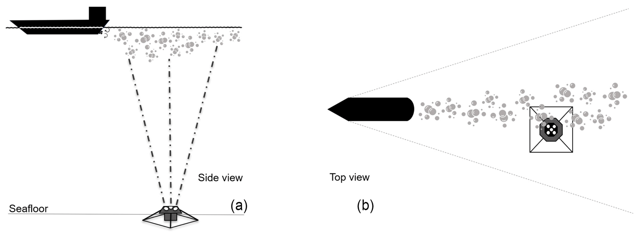
Figure 2 Scheme of instrument deployment, showing (a) the side view with a perspective of the ADCP placed on the seafloor facing upward and recording the turbulent wakes during ship passages and (b) a top-view perspective of the ADCP recording bubbles from a turbulent wake, induced by a ship passing above, but slightly to the side of the instrument.

A dataset of the ships passing the study area during the field measurement period was purchased from the Swedish Maritime Administration. The dataset is from the Baltic Marine Environment Protection Commission (HELCOM) automatic information system (AIS) database, which is processed according to the procedure described in the annex of the HELCOM Assessment on maritime activities in the Baltic Sea 2018 (HELCOM, 2018). The Swedish Institute for the Marine Environment (SIME) provided additional files from the same HELCOM database, with AIS data for the analysed satellite scenes and the Gothenburg harbour study area. Vessel information from MarineTraffic – Global Ship Tracking Intelligence (https://www.marinetraffic.com, last access: 15 October 2020) was used to retrieve detailed information about the width, length, and draught of the ships in the dataset.

2.1.2 Data analysis

The data analysis comprised detection and annotation of the turbulent wakes in the ADCP dataset, as well as statistical analysis of the final results. The analysis also included combining the in situ observations from the ADCP with the ship tracks and vessel information in the AIS dataset.

Compiling the ADCP wake dataset

All ship wakes in the dataset were identified manually using high-resolution figures of the echo amplitude of the ADCP beams (see Fig. 3 for an example). As the bubbles in the turbulent wake reflect the sound more efficiently than water, they induce an elevated echo amplitude in the turbulent wake region (NDRC, 1946; Marmorino and Trump, 1996; Trevorrow et al., 1994; Weber et al., 2005; Ermakov and Kapustin, 2010; Francisco et al., 2017). Generally, the wake signal could be clearly distinguished from bubbles induced by waves or signal noise from fish or zooplankton. However, ambiguous cases were noted, mainly during time periods with a lot of waves. Using a conservative approach, these cases were not considered wakes in the further analysis. Each wake in the dataset was linked to a ship track in the HELCOM AIS dataset, using manual comparison. This introduced additional uncertainties, as not all wakes had a clear match with a ship passage. Each ship in the AIS dataset passing within 184 m of the ADCP instrument was classified either as a wake-inducing passage or a no-wake passage. The wake-inducing passages included all ship passages where a clear wake was detected by the ADCP at the time of ship passage or after a slight delay (< 15 min). The no-wake passages included all passages without a detected wake, as well as all ambiguous wakes and unclear ship–wake matches. The distance at which a wake can be detected from a passing ship is affected by wake broadening, drifting, and ship width. In this study, the 184 m radius was chosen, as it was the furthest distance at which a clear wake and ship match was found in the dataset. Lastly, some wakes and passages were removed from the analysis altogether. These included ships with missing information in the AIS data (size information), clear wakes where two or three ships passed the instrument at the same time, making it impossible to discern which ship induced the detected wake, and small leisure boats

Distance calculation: AIS and ADCP dataset

The AIS dataset included position reports for each ship every 2–10 s, which were used to calculate the ship's track. The closest distance between the ship track and the vertical beam of the ADCP instrument was then calculated, using a local planar coordinate system, with the instrument at the origin. The coordinates for the closest point on the track was also calculated, using the Python GeoPy package function distance.distance, and the points just before and after the closest point on the track were then identified.

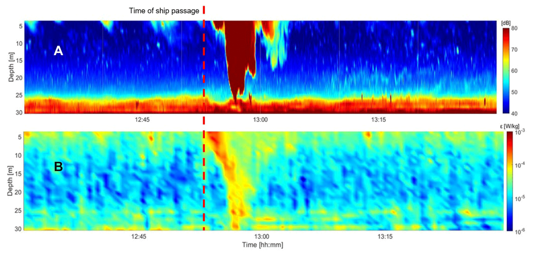
Figure 3 Example of the bubble wake signal in the echo amplitude dataset (a) and the calculated dissipation rate of turbulent kinetic energy, ε, (b) from 1 h of ADCP measurements. The upward-facing ADCP was placed at 32 m depth, repeatedly measuring the water column at one point. The dashed red line marks the time of ship passage. The high-intensity red (a) and yellow (b) areas after the ship passage represent the wake region. The increase in ε down to the bottom is evidence of increased turbulence and a vertical mixing down to 30 m depth. The wake was induced by a cargo ship (width 25 m, length 229 m, draught 7 m), which passed the instrument at a distance of 34 m and a speed of 19 kn.

Turbulence calculation: ADCP dataset

The dissipation rate of turbulent kinetic energy (ε) is a measure of the strength of the turbulence. By definition ε is the rate of energy conversion from kinetic energy to heat due to viscous friction in the smallest eddies, but in a stratified water column ε is also proportional to the mixing between different water masses. There are various ways of determining dissipation rates. In the present work ε is estimated from the ADCP data using the structure function method (e.g. Lucas et al., 2014), which estimates the dissipation rate of turbulent kinetic energy from the second-order structure function following Eq. (1):

$$\begin{array}{}\text{(1)}& D_{\mathrm{11}}\left(r,\mathrm{\Delta }r\right)=\stackrel{\mathrm{‾}}{{\left(u_r^{\prime }\left(r\right)-u_r^{\prime }\left(r+\mathrm{\Delta }r\right)\right)}^{\mathrm{2}}},\end{array}$$

where $u_r^{\prime }$ is the fluctuating velocity in the r direction (in this case the beam direction), Δr is the separation distance between two points along the beam, and the overbar denotes time averaging. For separation distances shorter than the largest eddies the structure function relates to the dissipation rate and separation distance as in Eq. (2):

$$\begin{array}{}\text{(2)}& D_{\mathrm{11}}\left(r,\mathrm{\Delta }r\right)=C{\mathit{\epsilon }}^{\mathrm{2}/\mathrm{3}}\mathrm{\Delta }{r}^{\mathrm{2}/\mathrm{3}},\end{array}$$

where C is a universal constant. Since the shortest distance (the ADCP bin size) was 1 m, the method is only expected to work for very strong turbulence with vertical eddy scales of magnitude larger than 2–3 m.

For each detected ship wake, the along-beam current velocity measurements from the ADCP were used for turbulence calculations in the wake region. One of the slanting beams was malfunctioning, but the four remaining beams were analysed. A 1 h dataset following each passage, identified by the start of the bubble cloud, was analysed. Spikes deviating more than 4 times the standard deviation from the mean in overlapping windows of 100 s length were removed. Since the velocity signal of surface waves at different depths may be expected to be coherent, whereas turbulent signals are not, the two empirical orthogonal function (EOF) modes with the largest variance were removed from the series to reduce the influence of surface waves. A fourth-order Butterworth high-pass filter with a cut-off period of 600 s was used to extract the turbulent velocity fluctuations. The dissipation rate of turbulent kinetic energy was estimated in 30 s bins (Lucas et al., 2014). One dissipation rate estimate was based on the average of the result for the three slanting beams (see Fig. 2 for an example), and another was based on the vertical beam.

Calculating wake depth, longevity, and maximum ε intensity: ADCP dataset

For each detected wake, the wake region was defined for the parameters echo amplitude (bubble wake), dissipation rate of turbulent kinetic energy (ε), and the maximum velocity variance. To reduce noise in the dataset induced by turbidity at the sea floor, the data were normalised with respect to vertical distance from the instrument, assuming exponential decay of the signal strength. The wake region was defined by visual scrutiny of echo amplitude and ε figures (see Fig. 2 for an example) and manually annotated. The elevation in echo amplitude or ε used for delimiting the wake region, as well as the depth and duration to consider, was manually adjusted for each wake to exclude noise. In general, the threshold was ∼ 15 % higher compared to the daily or nightly mean. The deepest part of the wake region was used as a measure of the maximum wake depth, and the maximum ε intensity in the wake region was used as a measure of the maximum turbulence. The duration of the wake (temporal longevity in min) was calculated using the start time and end time of the wake region. All calculations were pursued using an individually developed Python code.

Statistical analysis and graphical presentation of the ADCP wake dataset

The statistical analysis was performed for the entire wake dataset (all wakes) and for a subset including all wakes induced by ships passing within zero to three ship widths from the instrument (close wakes). This cut-off was chosen as there was a substantial decrease in the percentage of induced wakes at passages greater than three ship widths from the instrument, indicating difficulties in detecting wakes at larger distances. For both all wakes and the close wakes, the median wake depth (m) and temporal wake longevity (min) were calculated for the bubble wake and the ε dissipation rate wake, together with the standard deviation (SD) and the 25th and 75th percentile. Furthermore, the percentage of ship passages that induced a visible wake in the ADCP beams was calculated along with the maximum ε intensity in the wake region.

For the graphical presentation, the wake depth and longevity results are presented in relation to vessel force (F) [kg m s⁻²]. F was calculated from the ship width (B) [m], draught (T) [m], and speed (s) [m s⁻¹], as in Eq. (3):

$$\begin{array}{}\text{(3)}& F=\mathit{\rho }\cdot B\cdot T\cdot s^{\mathrm{2}},\end{array}$$

with seawater density (ρ) equal to 1025 kg m⁻³. The F parameter is proportional to ship drag and is used to relate the wake depth and longevity to vessel size and speed, which are parameters affecting the formation of the turbulent wake.

2.2 Bornholm satellite study

The Bornholm study area was chosen, as it covers the most intensely trafficked shipping lane in the Baltic Sea, with approximately 50 000 ship passages per year (HELCOM, 2010). All large ships heading for the eastern and northern ports of the Baltic Sea must use the Bornholm shipping lane (HELCOM, 2018), which makes it ideal for studying ship-induced vertical mixing from a variety of different ship types. Besides the purely traffic-related reason, the Bornholm area was favoured over the Gothenburg area based on the availability of cloud-free satellite scenes. A clear sky is essential for detecting any surface object in the optical and thermal wavelength, and for the investigated time period the Bornholm area (path 193/row 21) had 23 scenes with less than 23 % cloud cover above the sea, compared to the Gothenburg area (path 196/row 20) where only 9 scenes were available.

2.2.1 Data collection

All required optical and thermal infrared data from Landsat-8 were retrieved from https://s3-us-west-2.amazonaws.com, last access: 2 August 2019. The study area for the Bornholm area in the Baltic Sea was covered by path/row 193/21 (see Fig. 1 for an overview of study area).

2.2.2 Data analysis

The ships and thermal wakes in the satellite images were detected and annotated using a combination of automatised and manual analysis. The analysis included combining the detected thermal wakes with the ship tracks and vessel information in the AIS dataset, as well as statistical analysis of the results.

Compiling the satellite dataset

To obtain average wake lengths and widths indicating vertical mixing on regional scales, optical, near-infrared, and thermal-infrared bands from Landsat-8 were analysed. The dataset includes Landsat-8 data having a cloud cover < 23% (n=23). For optical and infrared data cloud coverage acts as opaque layer preventing us from inferring any information below it. The procedure includes a general and automatised data pre-processing scheme (Matlab), an automatic ship detection (Matlab), and a manual wake digitisation (ArcMap). The pre-processing encompasses (i) an automatic download of all available satellite scenes with less than 23 % cloud coverage of the given path/row, (ii) a masking of land areas using a combination of the modified normalised difference water index (MNDWI) after Xu (2006) and a Otsu-based threshold procedure (Otsu, 1979), (iii) a masking of opaque and cirrus clouds classified as such based on the CFMask (Foga et al., 2017), and (iv) finally a conversion from top-of-the-atmosphere (TOA) spectral radiances of band 10 to sea surface temperature (SST) using transmission, downwelling, and upwelling radiances modelled for each scene using a MODTRAN-based online tool (Barsi et al., 2003).

Detecting ships was pursued semi-automatically following an optical approach similar to the one described by Heiselberg (2016). After masking, the remaining and analysable area is open water only. Spectrally, ships can be differentiated using the visual and short-wave–infrared part of the spectrum, even on the basis of the coarser spatial resolution of 30 m as in the present case. As both parts of the spectrum are included in the MNDWI a global threshold of 0.09 was used on the MNDWI image for each scene to detect potential ships. To reduce the number of false positives due to unmasked cloud interference, a further selection criterion was added, using optical ship wake characteristics described in Gilman et al. (2011) and Heiselberg (2016), which is also visible in MNDWI space. Around all potential ships, a search window of 15×15 pixels (450×450 m) was created. If MNDWI values > 0.13 representing ship wakes were detected, the potential ship was converted to a true ship, while remaining potential ships were neglected.

Using the ships as a spatial indication, all available 23 scenes were screened for thermally indicated ship wakes. In the case of an occurrence, all thermal wakes for which a ship was detected were digitalised. Using this approach, the wake lengths were obtained (see Fig. 4 for an example of visible thermal wakes). To also retrieve wake widths, cross profiles were subsequently created at intervals of 250 m along the thermal ship wake, with a length of 400 m each. The cross-profile lengths were orientated at the maximum widths of < 300 m presented in Gilman et al. (2011). Wake width was automatically determined analysing the local temperature minima (thermal wake centre) and local temperature maxima (surrounding uninfluenced water area) for each of the cross profiles.

Combining the satellite wakes with AIS data

Identified wakes and ships from satellite data were automatically matched against AIS data to identify the ships inducing the wakes. All scenes were manually controlled to make sure the automatically matched ships were moving in the correct direction to have induced the wake. As the area of interest was the large shipping lane north-east of Bornholm, only the ships in the traffic-separated part of the shipping lane stretching from Bornholm to Öland's south tip were included in the analysis (see boxed area in Fig. 1c). In addition to the matched satellite ships, all other ships present in the area at the time of each satellite scene were identified.

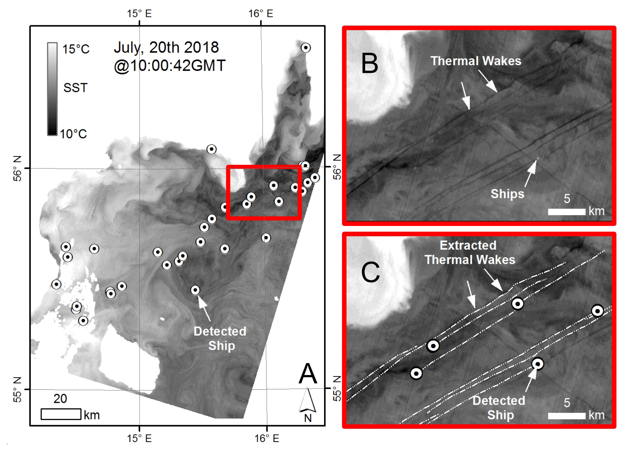
Figure 4 Example of satellite scene with visible thermal wakes in the Bornholm study area, with an illustration of the thermal wake detection process. Panel (a) is the original satellite scene with the detected ships marked as white circles with black dots. The red box marks the zoomed-in area in (b) and (c). In (b), the thermal wakes are visible as darker lines and the ships as small white dots. Panel (c) shows the detected ships and extracted thermal wakes. Landsat-8 image courtesy of the US Geological Survey.

Statistical analysis of satellite wake dataset

For the satellite dataset, the median spatial wake length (m) and wake width (m) were calculated, together with standard deviation (SD) and the 25th and 75th percentile. The percentage of ship passages inducing visible thermal wakes was also calculated.

3 Results and discussion

In the Gothenburg harbour study, there was a total of 68 detected turbulent wakes which could be successfully matched to a passing ship. In the Bornholm satellite image analysis, 144 thermal wakes were detected in the shipping lane area and successfully matched to a ship. Thus, a total of 212 ship wakes were included in the analysis, and the results from each study area will be presented separately below.

3.1 Gothenburg harbour study

During the measurement period, a total of 413 ships passed within 184 m of the ADCP instrument, of which 303 were included in the analysis. Of those passages, 68 (22 %) induced clearly visible wakes (all wakes), of which 38 (56 %) belonged to the subset of close-wake passages. The close-wake passages had a median passing distance of 29 m and a maximum of 82 m. The observed wake depth and longevity for the close wakes are presented in Sect. 3.1.4 and 3.1.5, and the results for all wakes are presented in the Supplement.

3.1.1 Environmental parameters

At the time of deployment, there was clear stratification at 10 m depth, with an upper mixed layer salinity of 25.5 and a gradual increase in salinity below the stratification, reaching a maximum salinity of 32 at 32 m depth (Fig. 5). The temperature profile showed a rather uniform profile, with only a slight increase towards the surface, indicating that salinity was the main stratifying component (Fig. 5). The surface layer had a temperature of 18–18.6 ^∘C, the middle layer ranged from 17.6 ^∘C at 10 m to 17.3 ^∘C at 20 m, and the deepest layer went from 17.4 ^∘C to 16.4 at the sea floor. At the time of instrument retrieval, there was only one clear pycnocline at 5 m depth, with an upper mixed layer temperature around 14 ^∘C and salinity around 27. The temperature below the pycnocline was around 16 ^∘C and the salinity was 33. This type of structure is usual in this area, as the Baltic Surface current, which brings low-salinity water from the Baltic Sea, is on top of the more saline water from the Skagerrak (Andersson and Rydberg, 1993). Note that the water column is unstable in temperature, so salinity is the stratifying component here too.

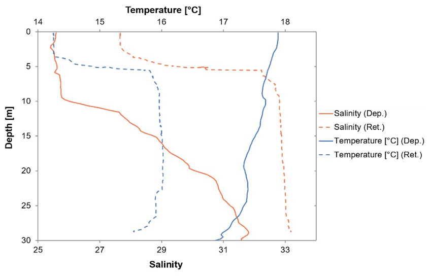
Figure 5 Salinity and temperature at the time of instrument deployment (28 August 2018; solid lines) and retrieval (25 September 2018; dashed lines).

3.1.2 Wake detection rate

For the close-wake subset, the detection rate ranged between 36 %–100 %, with an average of 56 % (Fig. 6). At distances greater than three ship widths, the wake detection was much lower (0 %–26 %) with an average of 13 %. Surprisingly, the detection rate of wakes induced by ships passing at distances greater than three ship widths does not seem to be affected by the vessel force, as the percentage of detected wakes is similar for all force bins (Fig. 6). Similarly, the close-wake category does not show a clear correlation between vessel force and wake detection rate. However, more passages with large vessel force would be needed to be able to draw any conclusions regarding the influence of vessel force on wake detection, since the data are skewed towards lower vessel forces. Nevertheless, the results presented in Fig. 6 indicate that passing distance affects the wake detection rate more than the vessel force.

3.1.3 Maximum wake depth

The median maximum wake depth for the close wakes was 11.5 m (SD 4.3 m) for the bubble wake and 13.5 m (SD 3.7 m) for the ε wake (Table 2). These ε wake depths were not the lower weak rim of the wake, as the threshold values defining the wake region mostly ranged between 10⁻⁴–10^−3.5 W kg⁻¹. These threshold values are large (e.g. Thorpe, 2007), indicating vigorously turbulent wakes, which were probably homogeneous down to the maximum depths of the wake region. Previous peer-reviewed studies have mainly reported turbulent wake depths of 8–12 m, with two observations from the grey literature of wake depths of 18 m (Table 1). The deepest detected wakes reached values of 27.5 m for the bubble wakes and 30.5 m for the ε wake. These maximum values are > 10 m deeper than previously reported depths in the grey literature and > 15 m deeper than previously reported in peer-reviewed studies (Table 1). The wakes detected from ships passing more than three ship widths from the instrument does not give a full representation of the maximum wake depth or longevity, as they likely represent the outer edges of the wake region. Nevertheless, these observations still provide information about the wake depth 3–55 ship widths from the wake centre (30–180 m), and the observed median values were 7.5 and 9.5 m for the bubble wakes and ε wakes respectively (Supplement Table S1).

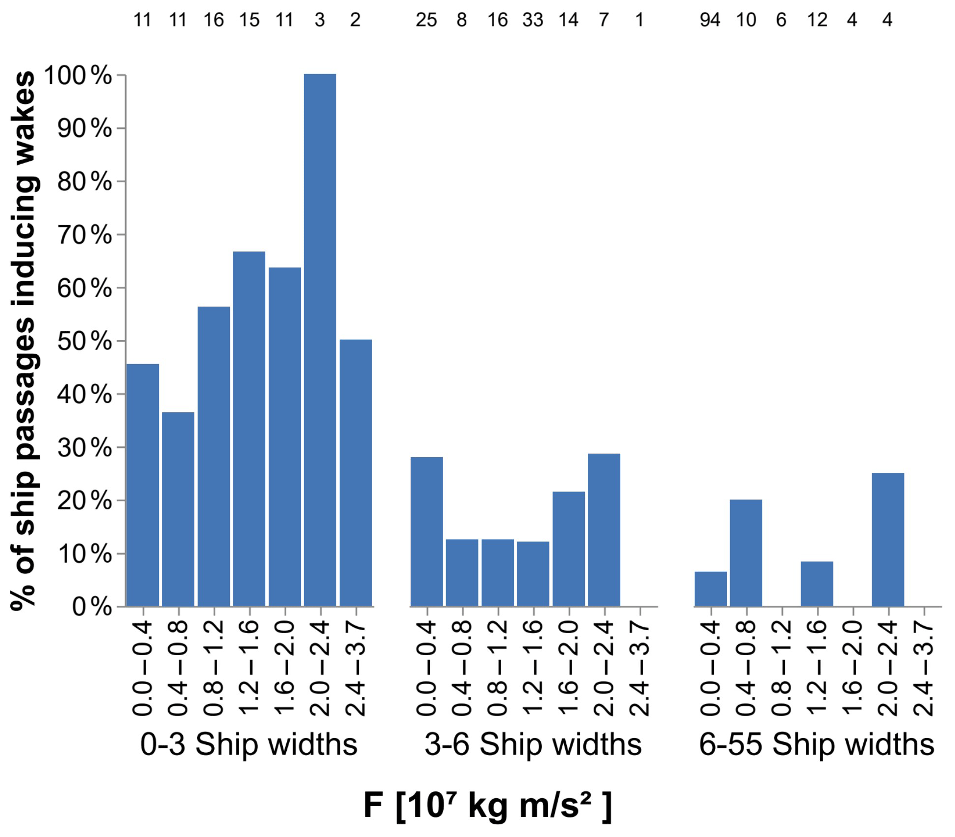
Figure 6 Wake occurrence for three different passing distances: 0–3, 3–6, and 6–55 ship widths from the instrument. For each distance, the x axis shows the force (F) of the passing vessel in newton. The number above each bar indicate the total number of passages for that passing distance. Note the cut-off in percentage of detected wakes at passing distances greater than three ship widths.

Table 2 Mean, median, and maximum value, first quartile (Q₂₅), third quartile (Q₇₅), and standard deviation (SD) for wake depth and longevity for the observed wakes induced by ships passing zero to three ship widths from the ADCP instrument.

In Fig. 7, the maximum wake depth is presented for the bubble wake and ε wake, in relation to vessel force (F). For the bubble wake, the percentage of induced wakes deeper than 12 m increases with increased vessel force (Fig. 7a), and there was a similar tendency for the ε wake (Fig. 7b). However, there was no statistically significant correlation between F and maximum wake depth for either category. The lack of correlation could partly be explained by the skewed data distribution, as there were few passages with a large F (Fig. 6).

Comparing the median maximum wake depth for the bubble wake and the ε wake, the ε wake was slightly deeper (∼2 m) (Table 2, Fig. 7). The bubbles in the wake are an indication of surface water being mixed down at depth and that it has been mixed with the ambient water. The bubbles will remain in the water column, or they can rise or collapse with time, depending on the bubble size. Bubbles with positive buoyancy will have an upward motion counteracting the downward mixing, which could be one explanation as to why the bubble wakes are slightly shallower than the ε wakes. The dissipation rate of turbulent kinetic energy, on the other hand, is a measure of the turbulent motions in the water that mixes the water down. When the turbulence decays, the dissipation also decays and dies out. The bubbles may remain after the turbulence has died out, which may explain why the bubble wake lasts longer compared to the ε wake. Another possible explanation to why the ε wakes are deeper is the calculation method used. The dissipation estimate is influenced by neighbouring cells (Eq. 1) and if there is strong turbulence in one cell and none in the next, the method may still show some turbulence in the calm cell.

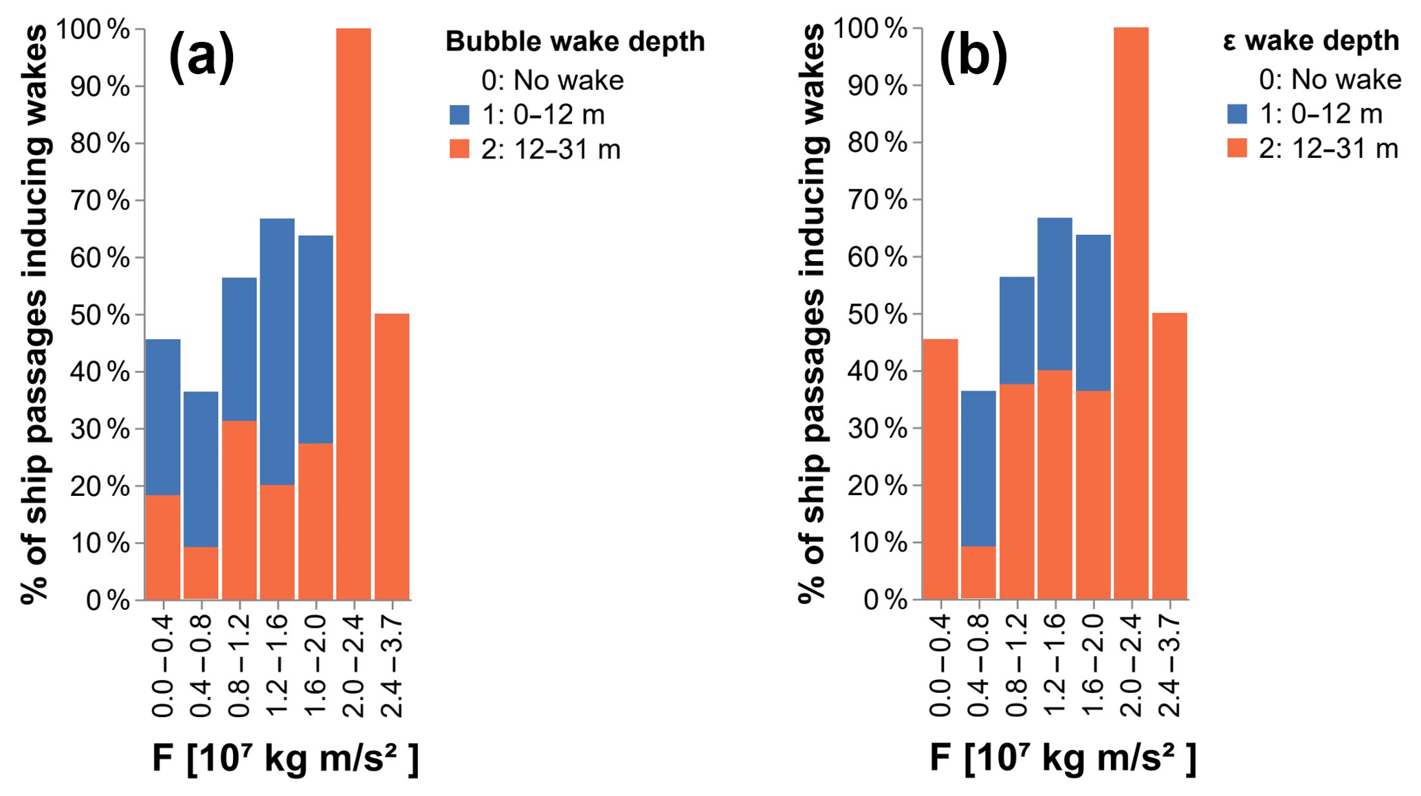
Figure 7 Maximum wake depth for the bubble wake (a) and dissipation rate of turbulent kinetic energy (ε) wake (b) for detected wakes induced by ships passing at zero to three ship widths from the instrument. The x axis shows the force (F) of the vessel in newton. Wake depths within the range presented in previous peer-reviewed studies are shown in blue, and wakes deeper than previously reported are shown in orange.

Among the ADCP measurements, there were a few wakes which reached depths of > 18 m (Table 2). The deepest wake, > 30 m, observed in this dataset was induced by a cargo ship with a beam of 25 m, length of 229 m, and draught of 7 m. The ship passed the instrument at a distance of 34 m and a speed of 19 kn. The cargo ship had a gross tonnage similar to the average of container and ro-ro cargo ships in the Baltic Sea (HELCOM, 2018), indicating that ship-induced mixing to depths of 30 m could be a common but undetected occurrence. The hypothesis that vertical mixing to this depth could be more frequent than expected from previous studies (Table 2) is supported by the observations that similarly sized ships passing at the same distance as the cargo ship inducing the deepest wake also induced mixing to depths greater than 15 m. On the other hand, the difference in wake depth for ships of similar size and passing distance could also be due to differences in stratification, as strong stratification can dampen the vertical development of the wake (Kato and Phillips, 1969). During the ADCP measurement campaign, water column stratification was measured at deployment and retrieval of the instrument (Fig. 4). Three hours before the instrument retrieval, a cargo ship passed at a distance of 21 m and induced a bubble wake of 13.5 m depth and an εwake 17.5 m depth. The CTD measurements 3 h later showed strong thermal stratification at 5 m depth. This indicates that during the time of ship passage, the turbulent wake must have mixed water across the thermocline. That the water is not homogeneous due to mixing 3 h after ship passage is not evidence that mixing is unimportant but just exemplifies why it is difficult to measure vessel-based mixing with standard instruments. After an intense localised mixing event in stratified water, the water will restratify (e.g. Arneborg, 2002), and the mixed water will spread out laterally. However, the effect of the mixing is irreversible, and its influence on physical, chemical, and biological properties is completed, although difficult to observe after restratification. Ship-induced turbulence interacts with the local and regional stratification, even though the contribution from each single ship is difficult to observe after the water has restratified. The lack of previous reports of vertical mixing of this magnitude can partly be explained by the fact that no previous study has targeted this specific research question. Moreover, measurements made using similar methods, but for other purposes, are seldom conducted in shipping lanes and particularly not from below. Further studies are needed to determine the interaction between stratification and the vertical development of the turbulent wake and the importance of the ship's draught and speed. The results of this study show that vertical mixing to depths down to 30 m occurs, and possibly at a high frequency, but current knowledge about the wake distribution is poor (especially on a vertical scale), and further studies are needed to determine when, and at what frequency, vertical mixing reaching this depth occurs.

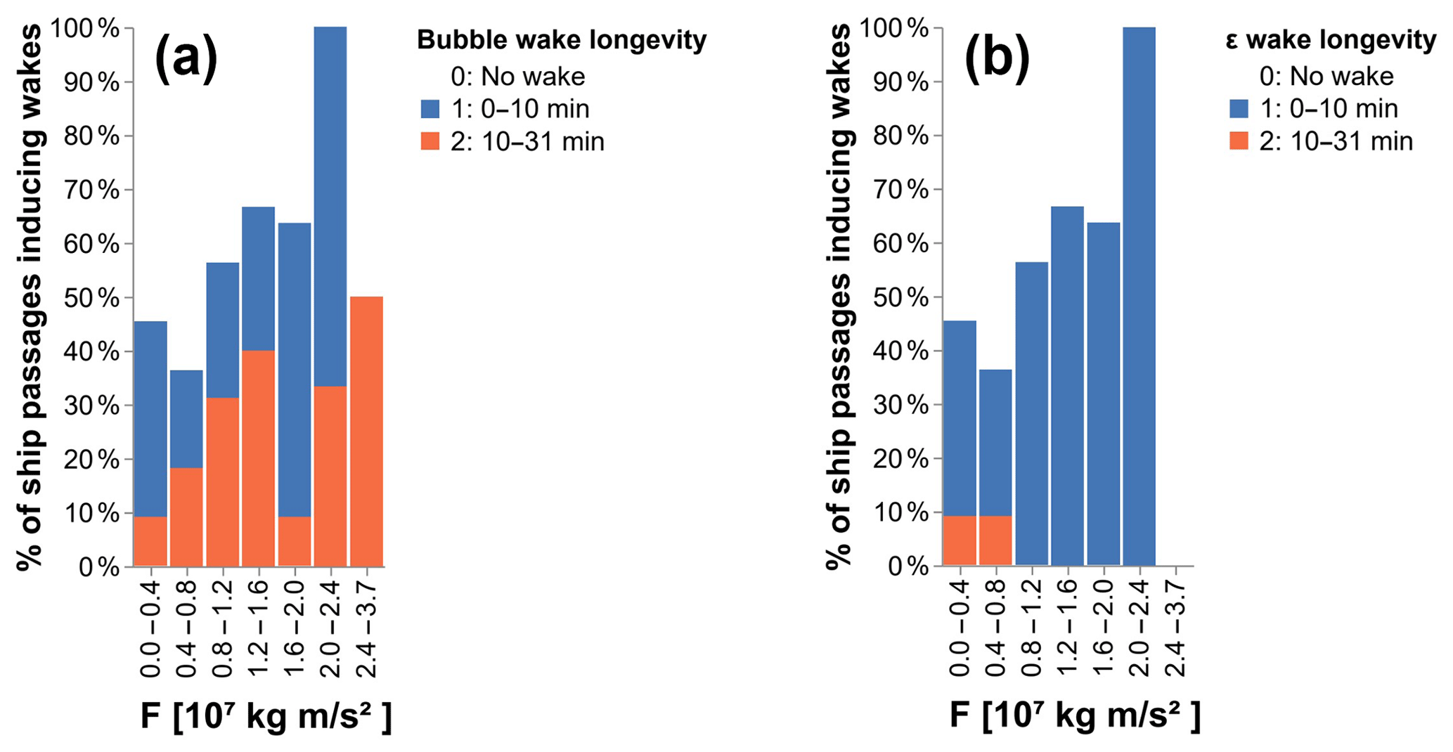
Figure 8 Wake longevity for the bubble wake (a) and dissipation rate of turbulent kinetic energy (ε) wake (b), for detected wakes induced by ships passing at zero to three ship widths from the instrument. The x axis shows the force (F) of the vessel in newton. Wake temporal longevities < 10 min are shown in blue, and wake longevities 10–31 min are shown in orange.

3.1.4 Wake temporal longevity

Figure 8 shows the wake temporal longevity related to vessel force for the bubble wake and ε wake. The median longevity was 9 min 59 s (SD 6 min 34 s) and 5 min 59 s (SD 2 min 33 s) for the bubble and ε wake respectively (Table 2). Figure 8 shows no clear correlation between wake longevity and vessel force for the bubble or ε wake. Hence, the results from this study indicate that parameters related to the vessel speed and size do not explain the variation in wake longevity to a very high degree. However, the relatively low number of passages with a large vessel force makes it difficult to draw any definite conclusions without further studies.

A detectable signal of the bubble wake from 10 and up to 30 min, is in agreement with previous studies (Table 1). Furthermore, the timescale of the wake longevity indicates that in highly trafficked areas, where large ships pass every 10–15 min, there is a high potential of a constant influence of ship-induced vertical mixing.

3.2 Bornholm satellite image analysis

There was a total of 94 satellite scenes from the period April 2013 to December 2018. Of these scenes, 25 % had a cloud cover of < 23 %, and were analysed for thermal wakes. Of these, 48 % (n=11) had visible thermal wakes. The monthly distribution of ship passages and occurrence of thermal wakes are shown in Fig. 9. As the number of analysed satellite scenes differed between months, the total number of ship passages for each month was divided by the number of analysed scenes. For all months, the majority of the passages did not induce visible thermal wakes. In April–July, there were several induced thermal wakes per scenes (Fig. 9), most of them in May and June. Occasional thermal wakes were found in September and October, but none were found during the winter months (December–February). In the satellite scenes where thermal wakes were visible and the environmental conditions were right for thermal wakes to be visible, 21 % of the ship passages induced thermal wakes (Table 3). For all the satellite scenes, including those without environmental conditions appropriate for inducing visible thermal wakes, 10 % of the ship passages induced thermal wakes.

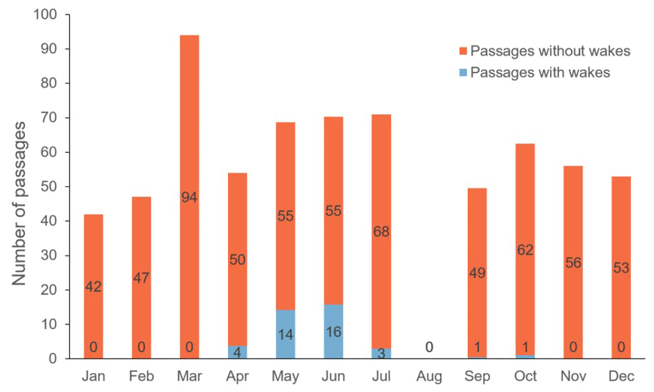
Figure 9 Seasonal distribution of ship passages for the satellite scenes with < 23 % cloud cover, for the period April 2013 to December 2018. The data labels in the stacked bar indicate the number of passages in each category. As some months have more than one analysed scene, the total number of ship passages for each month was divided by the number of analysed scenes to get an average number of passages per scene for each month. August had no scenes with < 23 % cloud cover and therefore has no data.

Table 3 Number of ship passages in the analysed satellite scenes and the percentage of passages inducing thermal wakes.

3.2.1 Spatial wake length

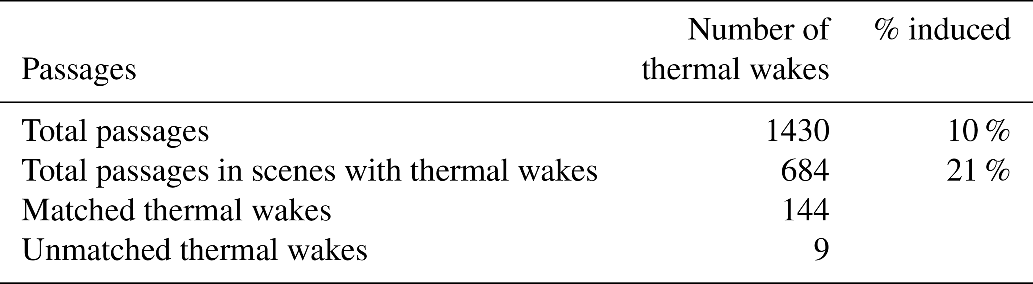
The median length of the matched thermal wakes in the shipping lane area was 13.7 km (SD 11.8 km), and 25 % were ≥ 20.9 km (Fig. 10a). Assuming that the median speed of the wake-inducing ships in the dataset (13.0 kn) is representative of the ship speed in the area, the calculated temporal wake longevity for the median wake length of 13.7 km was 34 min. The longest thermal wake was 62.5 km, which, considering the speed of the wake-inducing ship (20 kn), corresponds to a longevity of 1 h 42 min. In model experiments by Voropayev et al. (2012), the thermal wake signature was still increasing at a distance of 30 ship lengths behind the ship, which would correspond to 6 km for a 200 m long ship. Thus, the thermal wake length reported in the current study is up to 1 order of magnitude larger than previously reported experimental results, indicating an underestimation of thermal wake length in previous studies.

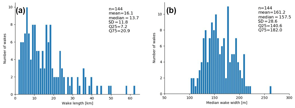
Figure 10 Distribution of observed thermal wake lengths (a) and widths (b), in the shipping lane area indicated in Fig. 1c. The observations are from satellite scenes with visible thermal wakes and <23 % cloud cover, for the period April 2013 to December 2018 (n=144).

3.2.2 Spatial wake width

The thermal wake width distribution is presented in Figs. 10b and 11. The median wake width for the entire dataset was 157.5 m (SD 28.6), which is within the 10–250 m range presented in previous studies (Table 1). There was no correlation between vessel width, length, or force [N] versus thermal ship wake width or length (data not shown). The width in this study corresponds to the values presented in Gilman et al. (2011), who used a ship-based remote-sensing approach to estimate width from the visible wake on the sea surface. In contrast, Trevorrow et al. (1994) and Ermakov and Kapustin (2010) reported typical widths of 40–80 m, which is narrower than any widths detected in the current study. However, the last two studies used acoustic measurements of bubbles to estimate the wake width, which could explain the diverging results. The distribution of the median wake width for the different satellite scenes can be seen in Fig. 11. Variations in stratification conditions could be one of the explanations as to why the thermal wake width varied between scenes. Another reason could be local and regional wind conditions as pointed out in Gilman et al. (2011) or simply the varying temperature gradient between entrained cooler temperatures and warmer temperatures of the upper layer and the resulting exponential adjustment process given Newton's law of cooling (Vollmer, 2009; Mallast and Siebert, 2019).

Figure 11 Median wake width distribution for the thermal wakes in the 11 satellite scenes with visible thermal wakes and < 23 % cloud cover, for the period April 2013 to December 2018. The median values are indicated with an “X”. The lower and upper edges of the box represent the 25th and 75th percentile of the dataset, and the entire box represents the interquartile range (IQR). The top whisker extends to the largest value within a distance of ≤ 1.5 times the IQR from the upper edge of the box, and the bottom whisker extends to the smallest value within a distance of ≤ 1.5 times the IQR of the lower edge of the box. Values at a distance > 1.5 times the IQR from the box edges are considered outliers and indicated by rings (∘).

3.3 Possible environmental implications of turbulent wakes

To put the effect of turbulent wakes at the observed spatiotemporal scales in the context of possible environmental implications, an example from the Bornholm area can be used. The traffic-separated shipping lane in the sound north of Bornholm is intensely trafficked, with 50 000 ship passages every year (HELCOM, 2010). Zooming into the shipping lane area and the traffic separation zones (each 5 km wide and ca. 30 km long), there are typically four to five ships present in each direction, at any given time (Fig. 12). Using the longevity and width of the “median” thermal wake as a proxy for the effect of the turbulent wake, the area of the shipping lane being affected by the turbulent wake, at any given time, can be estimated. Considering a scenario where all four wakes are uniformly distributed without overlap (Fig. 12), with a median thermal wake length of 13.7 km and width of 157.5 m (Fig. 9), the thermal wake area would be 8.6 km², i.e. 5.8 % of the shipping lane. However, considering the frequent ship traffic in the Bornholm sound, the presence of eight ships in each separation zone at the same time should occur frequently, implying 11.5 % thermal wake coverage.

In addition to the estimate of the area affected by the turbulent wake through its thermal signature, it is also possible to consider the frequency at which the water mass at a certain point would be influenced by a turbulent wake. An average of 50 000 ship passages in the Bornholm sound corresponds to 25 000 passages in each direction, corresponding to approximately one passage every 21 min (∼ three per hour), considering a scenario where all ships travel along the exact same path. The calculated median temporal thermal wake longevity for the satellite data was 34 min. As the thermal wake longevity is longer than the average time between ship passages, the assumption that all ships travel the exact same route would mean that the water mass along the travelled route would be under constant influence of a ship-induced thermal wake. The same scenario can also be assessed using the median temporal longevity for all the ADCP wake measurements from the close-wake passages: 9 min 59 s for the bubble wake and 5 min 59 s for the ε wake (Table 2). The assumption that there is a ship passage every 21 min means that there is 11 min between each ship passage when there are no bubbles; i.e. the shipping lane will be influenced close to 50 % of the time. If using the median temporal longevity for the ε wake instead, the shipping lane would be influenced close to 30 % of the time (15 min intervals without turbulence).

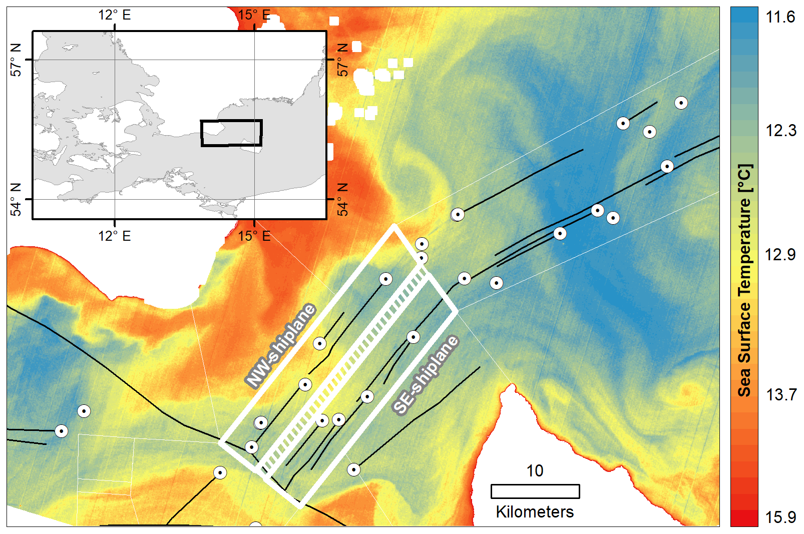
Figure 12 Ships and visible thermal wakes in the Bornholm sound from the analysed satellite scene from 25 May 2014 10:01 LT. White circles with black dots indicate ships with an AIS transmitter present in the area at the time of the satellite passage, and the black lines are the digitalised visible thermal wakes from the satellite scene. White lines indicate the shipping lane area, the bold lines mark the north-west and south-east shipping lanes, and the hatched area is the traffic separation zone. Landsat-8 image courtesy of the US Geological Survey.

The above calculated area coverage of thermal wakes and the frequency at which the water mass at a certain point would be influenced by ship-induced mixing represent two extremes. The first scenario assumes a uniform distribution of all ship wakes, and the second scenario assumes that all ships travel along the same route. However, in reality some of the wake regions would be overlapping (e.g. see Fig. 12), and most ships would travel similar but slightly different routes in the shipping lane. Nevertheless, based on the results presented in this study, areas like the Bornholm shipping lane in the Baltic Sea could be considered to be under a near-constant influence from ship-induced turbulent mixing. Even if the water column regained its stratification quite quickly, the mixing of the wake water with the surrounding water would take much longer (Arneborg, 2002). In a natural marine system, the water column is often stratified due to surface heating and/or freshwater influence. The wake turbulence interacts with this stratification by mixing the water and entraining deeper waters into the wake. The stratification may, in turn, reduce the vertical extent of the wake relative to what it would have been in a homogeneous water column (e.g. Voropayev et al., 2012). During periods of seasonal stratification, nutrients in the surface layer are depleted, and the supply of nutrients from below is limited due to damping of the vertical mixing by the stratification (Reissmann et al., 2009; Snoeijs-Leijonmalm and Andrén, 2017). In coastal regions, nutrients can be brought up to the upper mixed layer by coastal upwelling, but in open water, the nutrient supply is dependent on vertical mixing (Reissmann et al., 2009). If the vertical mixing is intense and deep enough, the mixing will bring up nutrient-rich water from below the stratification to the upper surface layer, which can increase primary production and sustain algal blooms. In ocean systems unaffected by human activities, vertical mixing in the surface layer is induced by wind, and the depth of the mixing depends on the wind strength and duration as well as the input of buoyancy from heating and freshwater (Thorpe, 2007). In temperate oceans like the Baltic Sea, the seasonal thermal stratification, at 10–20 m depth (Stigebrandt, 2001; Leppäranta and Myrberg, 2009), occurs during the summer season, which is also the period with the least wind (Reissmann et al., 2009). Thus, in unaffected seasonally stratified waters, there is little vertical mixing during the summer months. However, in areas with intense ship traffic there is a frequent input of ship-induced vertical mixing. In the Baltic Sea, at any given moment, there are circa 2000 moving vessels (HELCOM, 2010). A scoping calculation based on the average main engine power and velocity per ship type presented in Jalkanen et al. (2014) and the yearly distance travelled by each ship type from Hassellöv et al. (2019) will give a total input of turbulent kinetic energy from ship wakes of 3.9 GW. Using the conservative assumptions (1) that the ships are running at 50 % maximum continuous rating (MCR) (Buhaug et al., 2009; Smith et al., 2015) and (2) that the ships are operating evenly distributed on the total surface area of the Baltic Sea (including Kattegat and Skagerrak), the average energy input from turbulent ship wakes would be 0.0044 W m⁻². This ship-induced turbulent kinetic energy will mostly dissipate, but a certain fraction will be used to mix the water column in the case of stratified water. This can be compared with the dissipation rate of turbulent kinetic energy caused by wind- and wave-generated turbulence. Below the direct wave breaking layer, about one wave height thick (e.g. Sutherland and Melville, 2015), the dissipation rate of turbulent kinetic energy follows the “law of the wall” (Thorpe, 2007). There, the integrated dissipation rate of turbulent kinetic energy between the depths z₁ and z₂ can be written as Eq. (4):

$$\begin{array}{}\text{(4)}& {\mathit{\rho }}_{\mathrm{0}}{\displaystyle \frac{u_{\ast }^{\mathrm{3}}}{\mathit{\kappa }}}\ln {\displaystyle \frac{z_{\mathrm{2}}}{z_{\mathrm{1}}}},\end{array}$$

where ρ₀ is the water density, κ is the von Kármán constant (≅ 0.4), and u_∗ is the friction velocity. The friction velocity can be estimated from the wind velocity at 10 m height (U₁₀) as Eq. (5):

$$\begin{array}{}\text{(5)}& u_{\ast }=\sqrt{{\displaystyle \frac{{\mathit{\rho }}_{\mathrm{a}}}{{\mathit{\rho }}_{\mathrm{0}}}}{C}_{\mathrm{D}}}{U}_{\mathrm{10}},\end{array}$$

where ρ_a is the air density and C_D is a drag coefficient. An estimate of the integrated wind-generated dissipation rate at Gotska Sandön in the Baltic Sea between 1 and 20 m depth gives 0.002 W m⁻² in summer time and 0.007 W m⁻² in wintertime, based on wind observations and using the parameterisation of Smith (1988) for the drag coefficient. The dissipation rate of turbulent kinetic energy caused by vessels is therefore double the size of that caused by winds during summer at the depths where the turbulence may cause mixing of the seasonal thermocline. That is when averaged over the whole basin. The local impact in shipping lanes and behind individual ships is much larger. The Baltic Sea seasonal thermal stratification is located at 10–20 m depth (Stigebrandt, 2001; Leppäranta and Myrberg, 2009), and in many of the areas where the major shipping lanes are situated, the median water depth is between 20–50 m (Jakobsson et al., 2019). Consequently, during summer stratification, ship-induced turbulent mixing has a large potential to alter nutrient availability and gas exchange on a local to regional scale, which should be considered when evaluating environmental impact from shipping.

The results presented in this study also have implications for monitoring and data collection in areas with ship traffic, particularly when using FerryBox systems to conduct automated continuous measurements of parameters such as O₂ concentration, salinity, temperature, and sometimes also pCO₂, Chlorophyll a, and pigments (Petersen, 2014). In the Baltic Sea there are currently seven passenger ferries equipped with FerryBox systems, travelling along the major shipping lanes all or part of the journey (https://www.ferrybox.com/routes_data/routes/baltic_sea/index.php.en, last access: 15 October 2020). The intake of water to the FerryBox is from an inlet in the ship hull, located at approximately 2–10 m depth (Petersen, 2014). Considering the wake longevity of the thermal and turbulent wake observations presented in this study, there is a high likelihood that a ship travelling in a major shipping lane could be moving in the wake of another ship. In that case, the water being analysed by the FerryBox is the water of the turbulent wake and thus not necessarily representative of the conditions outside the shipping lane. Karlson et al. (2016) performed validations of FerryBox data, which were in good agreement with data from discrete water sampling in the shipping lane. Although the analytical precision and accuracy between the two methods seem to be good, the representativeness of both methods may be biased by turbulent wakes, as the validation was carried out within the shipping lane. Considering the general uncertainty of, e.g., seawater temperature measurements being in the order of 0.0025 K (e.g. Schmidt, 2016), the measured temperature differences, up to 1 ^∘C, between inside and outside the thermal wakes, (e.g. Fig. 4) could increase the uncertainty of the temperature measurements in the FerryBox data significantly. Further, as the bubbly wake affects gas exchange and saturation, it is important to know if the measurements are affected by ship-induced turbulence. Hence, the effect of ship-induced vertical mixing should be considered when using data collected from FerryBox systems.

3.4 Limitations and future outlook

The ADCP and satellite observations were used to capture different aspects of the turbulent wake, in order to estimate the entire spatiotemporal extent of the turbulent wake. As the thermal wakes show the effect of mixing, while ADCP observations show the actual turbulence that causes the mixing, the two approaches provide different but complementary results. The difference between the two methods, together with the separate geographical location, limits the possibilities of direct comparison and inference between the results. The observed longevity, for example, was expected to differ between the two approaches, as the turbulence will die out before the effect of the mixing of the water column has disappeared (thermal wake). For wake width, the satellite analysis showed a median wake width of 157.5 m (Fig. 10), implying that frequent detection of wakes from ships passing up to 75 m from the instrument would be expected. This wake width is within the range reported in previous studies (Table 2). The ADCP frequently detected wakes from ships passing within zero to three ship widths from the instrument (median of 29 m), indicating slightly narrower wake widths, although distances of up to 82 m were present within the close-wake subset. The large variation in vertical and horizontal distribution of the turbulent wakes observed during the wake analysis (inferred by comparing the signal between the slanted ADCP beams) strongly indicates that the vertical cross section across the width of the turbulent wake is non-uniform and varying. Based on these observations, the vertical cross section of the thermal wake is most likely also non-uniform and will differ in depth along the cross section. There is a need for further studies to clarify how the ship design, speed, and propeller (number and rotational direction) interact with water column stratification and currents in forming the “shape” of the turbulent wake.

The lack of detectable thermal wakes in the satellite dataset during the winter months was expected; for ship-induced turbulence to entrain cooler water from below and cause a surface temperature gradient, thermal stratification is needed. The Bornholm region usually has no thermal stratification during winter (Reissmann et al., 2009; van der Lee and Umlauf, 2011). Therefore, the method of estimating the spatiotemporal scales of the thermal wake using satellite SST observations is limited to seasons and regions where strong thermal stratifications occur. Moreover, the low percentage of available satellite scenes without too much cloud coverage, makes alternative remote-sensing techniques, such as drones, a possible alternative. Drones could also be used for longer time periods in the same area and in combination with underwater measurements.

As a current can move the wake towards or away from the instrument, the current speed and direction must be taken into consideration when estimating at what distance from the ship a wake is likely to be detected. Trevorrow et al. (1994) conducted measurements within 2–5 m of the turbulent wake and reported difficulties in catching the bubble signal from the wake using vertical sonars, as the wake often drifted out of the sonar range before it had completely dissipated. In this study, the water speed and waves were measured with the ADCP, and the wind effect on currents and waves was considered to have been captured by those measurements. A majority of the observed passages (50 %–60 %) occurred when there was a weak or no current at the position of the ADCP instrument (data not shown). Moreover, a current speed towards the instrument did not increase the likelihood of detecting the wake, especially not when ships passed further away from the instrument (data not shown).

In the current study, the water column stratification was only measured at deployment and retrieval of the instrument; hence the importance of stratification could not be addressed in this study. However, the presence and strength of the stratification will influence how much turbulence is required to mix water and substances across the thermocline (e.g. Kato and Phillips, 1969). In a stratified fluid, vertical mixing removes energy from the turbulence, reducing the vertical extent of the wake development. Stratification will also cause mixed fluid to spread out laterally, which causes an adjustment of the wake stratification to the surrounding stratification, resulting in a widening of the wake as well as an additional limitation of the vertical extent (Voropayev et al., 2012). As the aim of the current study was to present an order of magnitude estimation of the spatial and temporal scales of the turbulent wake, the lack of stratification measurements does not present an immediate problem within the current scope, yet it could be one explanation for the absence of statistically significant correlations between wake depth and vessel force. For future studies aiming at characterising the development of the turbulent wake and quantifying the ship-induced vertical mixing, stratification measurements will be necessary in order to understand the interaction between the stratification and the turbulent wake.

In shallow-water regimes the waves of the Kelvin wake give rise to increased current speeds at the sea floor, which can lead to resuspension (Soomere and Kask, 2003; Soomere, 2007). The measurements in this study also indicated resuspension and turbulence at the sea floor at 30 m depths, induced by the Kelvin wake from passing ships. These observations indicate the importance of including the effect of the Kelvin wake where shallow-water regimes apply when estimating the environmental impact on the marine environment in intensely trafficked shipping lanes. However, the effect of Kelvin wakes is outside the scope of the current study but has been investigated by Soomere and Kask (2003), Soomere (2007), and Soomere et al. (2009).

Finally, in order to determine when vertical mixing reaching depths of 30 m occurs and how common it is, future studies need to simultaneously measure the wake at more than one point to capture the 2D cross section, i.e. both the depth and the width of the wake. One way of achieving this would be to conduct measurements with several ADCPs placed on a row perpendicular to the shipping lane. Moreover, a line of instruments would also be able to capture a drifting wake and thus better estimate the true longevity. One of the limitations of the longevity estimation in this study is that currents could potentially shift the wake away from the instrument. Using multiple instruments would increase the chance of capturing the entire wake development, as it would cover a larger area, thus increasing the reliability of the longevity estimation. As the results from this study indicate that proximity is of importance for detecting the turbulent wakes using ADCP measurements, multiple instruments would increase the area where ships can pass close to the instrument. In addition, if the maximum depth of the wake is located only in a certain region of the turbulent wake, the likelihood of measuring that part of the wake is small when only one instrument is used. This spatial limitation of the current study makes it difficult to determine if the small number of detected deep wakes was because of low occurrence, or because using only one instrument made it difficult to successfully capture the deepest part of the wake. Thus, multiple instruments would increase the ability to identify when and where the very deep mixing occurs and shed further light upon how frequently deep mixing is induced. Conducting concurrent measurements using ADCPs and remote sensing would also be beneficial. In the current study, the satellite analysis and ADCP measurements have been conducted at different locations and time periods, but concurrent measurements would be necessary for obtaining a more complete picture of how the three-dimensional wakes develop for various combinations of stratification, vessel dimensions, propeller properties, and vessel speed.

4 Conclusions

Based on a large sample of in situ measurements, the median spatiotemporal extent of turbulent ship wakes has been estimated to a depth of 13.5 m and longevity of 9 min 59 s, based on ADCP measurements. Thermal wake width and length have been estimated to a median of 157.5 m and 13.7 km respectively, based on SST satellite image analysis. The results show frequent detection of turbulent wakes deeper than 12 m, which is deeper than previously reported. During summer, the total dissipation of turbulent kinetic energy induced by ships in the Baltic Sea is larger than that from wind-generated turbulence between 1 and 20 m depth. Wind mixing is homogeneously distributed over the Baltic Sea, whereas vessel mixing is concentrated in shipping lanes, implying that the local mixing from vessels is much larger than that from winds within the lanes. In these shipping lanes, satellite data show that the influence of vessel mixing covers a large fraction of the surface area, and our in situ turbulence data show that the mixing in the wakes has an influence at depths down to, typically, 14 m. Therefore, ship mixing should be considered when assessing environmental impacts from shipping. The potential bias of FerryBox measurements, e.g. up to 1 ^∘C temperature difference inside versus outside the shipping lane should also be further investigated.