the Creative Commons Attribution 4.0 License.
the Creative Commons Attribution 4.0 License.
 | 17 Jul 2020
An approach to the verification of high-resolution ocean models using spatial methods
Ric Crocker
Jan Maksymczuk
Marion Mittermaier
Marina Tonani
Christine Pequignet
The Met Office currently runs two operational ocean forecasting configurations for the North West European Shelf: an eddy-permitting model with a resolution of 7 km (AMM7) and an eddy-resolving model at 1.5 km (AMM15).
Whilst qualitative assessments have demonstrated the benefits brought by the increased resolution of AMM15, particularly in the ability to resolve finer-scale features, it has been difficult to show this quantitatively, especially in forecast mode. Applications of typical assessment metrics such as the root mean square error have been inconclusive, as the high-resolution model tends to be penalised more severely, referred to as the double-penalty effect. This effect occurs in point-to-point comparisons whereby features correctly forecast but misplaced with respect to the observations are penalised twice: once for not occurring at the observed location, and secondly for occurring at the forecast location, where they have not been observed.
An exploratory assessment of sea surface temperature (SST) has been made at in situ observation locations using a single-observation neighbourhood-forecast (SO-NF) spatial verification method known as the High-Resolution Assessment (HiRA) framework. The primary focus of the assessment was to capture important aspects of methodology to consider when applying the HiRA framework. Forecast grid points within neighbourhoods centred on the observing location are considered as pseudo ensemble members, so that typical ensemble and probabilistic forecast verification metrics such as the continuous ranked probability score (CRPS) can be utilised. It is found that through the application of HiRA it is possible to identify improvements in the higher-resolution model which were not apparent using typical grid-scale assessments.
This work suggests that future comparative assessments of ocean models with different resolutions would benefit from using HiRA as part of the evaluation process, as it gives a more equitable and appropriate reflection of model performance at higher resolutions.
- Article
(4128 KB) - Full-text XML
- BibTeX
- EndNote


When developing and improving forecast models, an important aspect is to assess whether model changes have truly improved the forecast. Assessment can be a mixture of subjective approaches, such as visualising forecasts and assessing whether the broad structure of a field is appropriate, or objective methods, comparing the difference between the forecast and an observed or analysed value of “truth” for the model domain.
Different types of intercomparison can be applied to identify the following different underlying behaviours:
-
between different forecasting systems over an overlapping region to check for model consistency between the two;
-
between two versions of the same model to test the value of model upgrades prior to operational implementation;
-
parent–son intercomparison, evaluating the impact of downscaling or nesting of models;
-
a forecast comparison against reanalysis of the same model, inferring the effect of resolution and forcing, especially in coastal areas.
There are a number of works which have used these types of assessment to delve into the characteristics of forecast models (e.g. Aznar et al., 2016; Mason et al., 2019; Juza et al., 2015) and produce coordinated validation approaches (Hernandez et al., 2015).
To aid the production of quality model assessment, services exist which regularly produce multi-model assessments to deliver to the ocean community (e.g. Lorente et al., 2019b).
One of the issues faced when assessing high-resolution models against lower-resolution models over the same domain is that often the coarser model appears to perform at least equivalently or better when using typical verification metrics such as root mean squared error (RMSE) or mean error, which is a measure of the bias. Whereas a higher-resolution model has the ability and requirement to forecast greater variation, detail and extremes, a coarser model cannot resolve the detail and will, by its nature, produce smoother features with less variation resulting in smaller errors. This can lead to the situation that despite the higher-resolution model looking more realistic it may verify worse (e.g. Mass et al., 2002; Tonani et al., 2019).
This is particularly the case when assessing forecast models categorically. If the location of a feature in the model is incorrect, then two penalties will be accrued: one for not forecasting the feature where it should have been and one for forecasting the same feature where it did not occur (the double-penalty effect, e.g. Rossa et al., 2008). This effect is more prevalent in higher-resolution models due to their ability to, at least, partially resolve smaller-scale features of interest. If the lower-resolution model could not resolve the feature and therefore did not forecast it, that model would only be penalised once. Therefore, despite giving potentially better guidance, the higher-resolution model will verify worse.
Yet, the underlying need to quantitatively show the value of high-resolution led to the development of so-called “spatial” verification methods which aimed to account for the fact the forecast produced realistic features that were not necessarily at the right place or at quite the right time (e.g. Ebert, 2008, or Gilleland, 2009). These methods have been in routine use within the atmospheric model community for a number of years with some long-term assessments and model comparisons (e.g. Mittermaier et al., 2013, for precipitation).
Spatial methods allow forecast models to be assessed with respect to several different types of focus. Initially, these methods were classified into four groups. Some methods look at the ability to forecast specific features (e.g. Davis et al., 2006); some look at how well the model performs at different scales (scale separation, e.g. Casati et al., 2004). Others look at field deformation (how much a field would have to be transformed to match a “truth” field (e.g. Keil and Craig, 2007). Finally, there is neighbourhood verification, many of which are equivalent to low-band-pass filters. In these methods, forecasts are assessed at multiple spatial or temporal scales to see how model skill changes as the scale is varied.
Dorninger et al. (2018) provides an updated classification of spatial methods, suggesting a fifth class of methods, known as distance metrics, which sit between field deformation and feature-based methods. These methods evaluate the distances between features, but instead of just calculating the difference in object centroids (which is typical), the distances between all grid point pairs are calculated, which makes distance metrics more similar to field deformation approaches. Furthermore, there is no prior identification of features. This makes distance metrics a distinct group that warrants being treated as such in terms of classification. Not all methods are easy to classify. An example of this is the integrated ice edge error (IIEE) developed for assessing the sea ice extent (Goessling et al., 2016).
This paper exploits the use of one such spatial technique for the verification of sea surface temperature (SST) in order to determine the levels of forecast accuracy and skill across a range of model resolutions. The High-Resolution Assessment framework (Mittermaier, 2014; Mittermaier and Csima, 2017) is applied to the Met Office Atlantic Margin Model running at 7 km (O'Dea et al., 2012, 2017; King et al., 2018) (AMM7) and 1.5 km (Graham et al., 2018; Tonani et al., 2019) (AMM15) resolutions for the North West European Shelf (NWS). The aim is to deliver an improved understanding beyond the use of basic biases and RMSEs for assessing higher-resolution ocean models, which would then better inform users on the quality of regional forecast products. Atmospheric science has been using high-resolution convective-scale models for over a decade and thus have experience in assessing forecast skill on these scales, so it is appropriate to trial these methods on eddy-resolving ocean model data. As part of the demonstration, the paper also looks at how the method should be applied to different ocean areas, where variation at different scales occurs due to underlying driving processes.
The paper was influenced by discussions on how to quantify the added value from investments in higher-resolution modelling given the issues around the double-penalty effect discussed above, which is currently an active area of research within the ocean community (Lorente et al., 2019a; Hernandez et al., 2018; Mourre et al., 2018).
Section 2 describes the model and observations used in this study along with the method applied. Section 3 presents the results, and Sect. 4 discusses the lessons learnt while using HiRA on ocean forecasts and sets the path for future work by detailing the potential and limitations of the method.
2.1 Forecasts
The forecast data used in this study are from the two products available in the Copernicus Marine Environment Monitoring Service (CMEMS; see, e.g. Le Traon et al., 2019, for a summary of the service) for the North West European Shelf area:
-
NORTHWESTSHELF_ANALYSIS_FORECAST_ PHYS_004_001_b (AMM7) and
-
NORTHWESTSHELF_ANALYSIS_FORECAST_ PHY_004_013 (AMM15).
The major difference between these two products is the horizontal resolution: ∼7 km for AMM7 and 1.5 km for AMM15. Both systems are based on a forecasting ocean assimilation model with tides. The ocean model is NEMO (Nucleus for European Modelling of the Ocean; Madec and the NEMO team, 2016), using the 3D-Var NEMOVAR system to assimilate observations (Mogensen et al., 2012). These are surface temperature in situ and satellite measurements, vertical profiles of temperature and salinity, and along-track satellite sea level anomaly data. The models are forced by lateral boundary conditions from the UK Met Office North Atlantic Ocean forecast model and by the CMEMS Baltic forecast product (BALTICSEA_ANALYSIS_FORECAST_PHY_003_006). The atmospheric forcing is given by the operational European Centre for Medium-Range Weather Forecasts (ECMWF) numerical weather prediction model for AMM15 and by the operational UK Met Office Global Atmospheric model for AMM7.
The AMM15 and AMM7 systems run once a day and provide forecasts for temperature, salinity, horizontal currents, sea level, mixed layer depth and bottom temperature. Hourly instantaneous values and daily 25 h de-tided averages are provided for the full water column.
AMM7 has a regular latitude–longitude grid, whilst AMM15 is computed on a rotated grid and regridded to have both models delivered to the (CMEMS) data catalogue (http://marine.copernicus.eu/services-portfolio/access-to-products/, last access: October 2019) on a regular grid. Table 1 provides a summary of the model configuration, a fuller description can be found in Tonani et al. (2019).
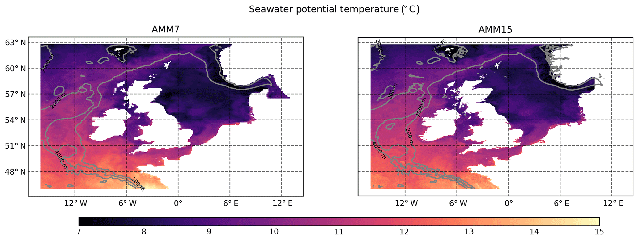
Figure 1AMM7 and AMM15 co-located areas. Note the difference in the land–sea boundaries due to the different resolutions, notably around the Scandinavian coast. Contours show the model bathymetry at 200, 2000 and 4000 m.
For the purpose of this assessment, the 5 d daily mean potential SST forecasts (with lead times of 12, 36, 60, 84 and 108 h) were utilised for the period from January to September 2019. Forecasts were compared for the co-located areas of AMM7 and AMM15. Figure 1 shows the AMM7 and AMM15 co-located domain along with the land–sea mask for each of the models. AMM15 has a more detailed coastline and SST field than AMM7 due to its higher resolution. When comparing two models with different resolutions, it is important to know whether increased detail actually translates into better forecast skill. Additionally, the differences in coastline representation can have an impact on any HiRA results obtained, as will be discussed in a later section.
It should be noted that this study is an assessment of the application of spatial methods to ocean forecast data and, as such, is not meant as a full and formal assessment and evaluation of the forecast skill of the AMM7 and AMM15 ocean configurations. To this end, a number of considerations have had to be taken into account in order to reduce the complexity of this initial study. Specifically, it was decided at an early stage to use daily mean SST temperatures, as opposed to hourly instantaneous SST, as this avoided any influence of the diurnal cycle and tides on any conclusions made. AMM15 and AMM7 daily means are calculated as means over 25 h to remove both the diurnal cycle and the tides. The tidal signal is removed because the period of the major tidal constituent, the semidiurnal lunar component M2, is 12 h and 25 min (Howarth and Pugh, 1983). Daily means are also one of the variables that are available from the majority of the products within the CMEMS catalogue, including reanalysis, so the application of the spatial methods could be relevant in other use cases beyond those considered here. In addition, there are differences in both the source and frequency of the air–sea interface forcing used in both the AMM7 and AMM15 configurations which could influence the results. Most notably, AMM7 uses hourly surface pressure and 10 m winds from the Met Office Unified Model (UM), whereas AMM15 uses 3-hourly data from ECMWF.

Figure 2Observation locations within the domain for 12:00 UTC on 6 June 2019.
2.2 Observations
SST observations used in the verification were downloaded from the CMEMS catalogue from the product
-
INSITU_NWS_NRT_OBSERVATIONS_013_036.
This dataset consists of in situ observations only, including daily drifters, mooring, ferry-box and conductivity–temperature–depth (CTD) observations. This results in a varying number of observations being available throughout the verification period, with uneven spatial coverage over the verification domain. Figure 2 shows a snapshot of the typical observational coverage, in this case for 12:00 UTC on 6 June 2019. This coverage is important when assessing the results, notably when thinking about the size and type of area over which an observation is meant to be representative of, and how close to the coastline each observation is.
This study was set up to detect issues that should be considered by users when applying HiRA within a routine ocean verification setup, using a broad assessment containing as much data as were available in order to understand the impact of using HiRA for ocean forecasts. Several assumptions were made in this study.
For example, there is a temporal mismatch between the forecasts and observations used. The forecasts (which were available at the time of this study) are daily means of the SSTs from 00:00 to 00:00 UTC, whilst the observations are instantaneous and usually available hourly. For the purposes of this assessment, we have focused on SSTs closest to the midpoint of the forecast period for each day (nominally 12:00 UTC). Observation times had to be within 90 min of this time, with any other times from the same observation site being rejected. A particular reason for picking a single observation time rather than daily averages was so that moving observations, such as drifting buoys, could be incorporated into the assessment. Creating daily mean observations from moving observations would involve averaging reports from different forecast grid boxes and hence contaminate the signal that HiRA is trying to evaluate.
Future applications would probably contain a stricter setup, e.g. only using fixed daily mean observations, or verifying instantaneous (hourly) forecasts so as to provide a subdaily assessment of the variable in question.
The HiRA framework (Mittermaier, 2014) was designed to overcome the difficulties encountered in assessing the skill of high-resolution models when evaluating against point observations. Traditional verification metrics such as RMSE and mean error rely on precise matching in space and time, by (typically) extracting the nearest model grid point to an observing location. The method is an example of a single-observation neighbourhood-forecast (SO-NF) approach, with no smoothing. All the forecast grid points within a neighbourhood centred on an observing location are treated as a pseudo ensemble, which is evaluated using well-known ensemble and probabilistic forecast metrics. Scores are computed for a range of (increasing) neighbourhood sizes to understand the scale–error relationship. This approach assumes that the observation is not only representative of its precise location but also has characteristics of the surrounding area. WMO manual No. 8 (World Meteorological Organisation, 2017) suggests that, in the atmosphere, observations can be considered representative of an area within a 100 km radius of a land station, but this is often very optimistic. The manual states further: “For small-scale or local applications the considered area may have dimensions of 10 km or less.” A similar principle applies to the ocean; i.e. observations can represent an area around the nominal observation location, though the representative scales are likely to be very different from in the atmosphere. The representative scale for an observation will also depend on local characteristics of the area, for example, whether the observation is on the shelf or in the open ocean or likely to be impacted by river discharge.
There will be a limit to the useful forecast neighbourhood size which can be used when comparing to a point observation. This maximum neighbourhood size will depend on the representative scale of the variable under consideration. Put differently, once the neighbourhoods become too big, there will be forecast values in the pseudo ensemble which will not be representative of the observation (and the local climatology) and any skill calculated will be essentially random. Combining results for multiple observations with very different representative scales (for example, a mixture of deep ocean and coastal observations) could contaminate results due to the forecast neighbourhood only being representative of a subset of the observations. The effect of this is explored later in this paper.
HiRA can be based on a range of statistics, data thresholds and neighbourhood sizes in order to assess a forecast model. When comparing deterministic models of different resolutions, the approach is to equalise on the physical area of the neighbourhoods (i.e. having the same “footprint”). By choosing sequences of neighbourhoods that provide (at least) approximate equivalent neighbourhoods (in terms of area), two or more models can be fairly compared.
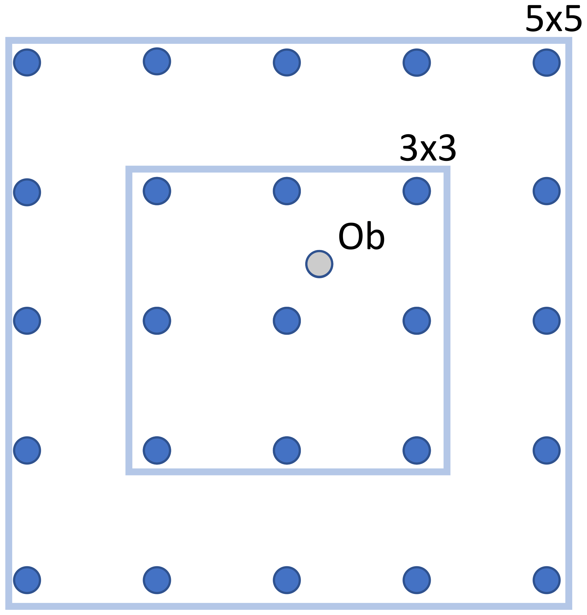
Figure 3Example of forecast grid point selections for different HiRA neighbourhoods for a single observation point. A 3×3 domain returns nine points that represent the nearest forecast grid points in a square around the observation. A 5×5 domain encompasses more points.
HiRA works as follows. For each observation, several neighbourhood sizes are constructed, representing the length in forecast grid points of a square domain around the observation points, centred on the grid point closest to the observation (Fig. 3). There is no interpolation applied to the forecast data to bring them to the observation point; all the data values are used unaltered.
Once neighbourhoods have been constructed, the data can be assessed using a range of well-known ensemble or probabilistic scores. The choice of statistic usually depends on the characteristics of the parameter being assessed. Parameters with significant thresholds can be assessed using the Brier score (Brier, 1950) or the ranked probability score (RPS) (Epstein, 1969), i.e. assessing the ability of the forecast to correctly locate a forecast in the correct threshold band. For continuous variables such as SST, the data have been assessed using the continuous ranked probability score (CRPS) (Brown, 1974; Hersbach, 2000).
The CRPS is a continuous extension of the RPS. Whereas the RPS is effectively an average of a user-defined set of Brier scores over a finite number of thresholds, the CRPS extends this by considering an integral over all possible thresholds. It lends itself well to ensemble forecasts of continuous variables such as temperature and has the useful property that the score reduces to the mean absolute error (MAE) for a single-grid-point deterministic model comparison. This means that, if required, both deterministic and probabilistic forecasts can be compared using the same score.
Equation (1) defines the CRPS, where for a parameter x, Pfcst(x) is the cumulative distribution of the neighbourhood forecast and Pobs(x) is the cumulative distribution of the observed value, represented by a Heaviside function (see Hersbach, 2000). The CRPS is an error-based score where a perfect forecast has a value of zero. It measures the difference between two cumulative distributions: a forecast distribution formed by ranking the (in this case, quasi)-ensemble members represented by the forecast values in the neighbourhood and a step function describing the observed state. To use an ensemble, HiRA makes the assumption that all grid points within a neighbourhood are equi-probable outcomes at the observing location. Therefore, aside from the observation representativeness limit, as the neighbourhood sizes increase, this assumption of equi-probability will break down as well, and scores become random. Care must therefore be taken to decide whether a particular neighbourhood size is appropriately representative. This decision will be based on the length scales appropriate for a variable as well as the resolution of the forecast model being assessed. Figure 4 shows a schematic of how different neighbourhood sizes contribute towards constructing forecast probability density functions around a single observation.
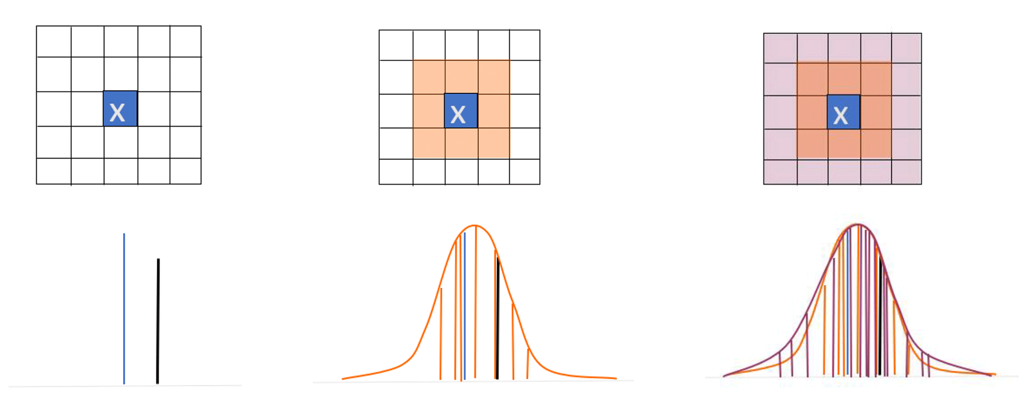
Figure 4Example of how different forecast neighbourhood sizes would contribute to the generation of a probability density function around an observation (denoted by x). The larger the neighbourhood, the better described the pdf, though potentially at the expense of larger spread. If a forecast point is invalid within the forecast neighbourhood, that site is rejected from the calculations for that neighbourhood size.
AMM7 and AMM15 resolve different length scales of motion due to their horizontal resolution. This should be taken into account when assessing the results of different neighbourhood sizes. Both models can resolve the large barotropic scale (∼200 km) and the shorter baroclinic scale off the shelf in deep water. On the continental shelf, only the resolution of ∼1.5 km of AMM15 permits motions at the smallest baroclinic scale since the first baroclinic Rossby radius is on the order of 4 km (O'Dea et al., 2012). AMM15 represents a step change in representing the eddy dynamics variability on the continental shelf. This difference has an impact also on the data assimilation scheme, where two horizontal correlation length scales (Mirouze et al., 2016) are used to represent large and small scales of ocean variability. The long length scale is 100 km, while the short correlation length scale aims to account for internal ocean processes variability, characterised by the Rossby radius of deformation. Computational requirements restrict the short length scale to be at least three model grid points, 4.5 and 21 km, respectively, for AMM15 and AMM7 (Tonani et al., 2019). Although AMM15 resolves smaller-scale processes, comparing AMM7 and AMM15 in neighbourhood sizes between the AMM7 resolution and multiples of this resolution will address processes that should be accounted for in both models.
As the methodology is based on ensemble and probabilistic metrics, it is naturally extensible to ensemble forecasts (see Mittermaier and Csima, 2017), which are currently being developed in research mode by the ocean community, allowing for intercomparison between deterministic and probabilistic forecast models in an equitable and consistent way.
Verification was performed using the Point-Stat tool, which is part of the Model Evaluation Tools (MET) verification package that was developed by the National Center for Atmospheric Research (NCAR) and which can be configured to generate CRPS results using the HiRA framework. MET is free to download from GitHub at https://github.com/NCAR/MET (last access: May 2019).
When comparing neighbourhoods between models, the preference is to look for similar-sized areas around an observation and then transform this to the closest odd-numbered square neighbourhood, which will be called the “equivalent neighbourhood”. In the case of the two models used, the most appropriate neighbourhood size can change depending on the structure of the grid, so the user needs to take into consideration what is an accurate match between the models being compared.
The two model configurations used in this assessment are provided on standard latitude–longitude grids via the CMEMS catalogue. The AMM7 and AMM15 configurations are stated to have resolutions approximating 7 and 1.5 km, respectively. Thus, equivalent neighbourhoods should simply be a case of matching neighbourhoods with similar spatial distances. In fact, AMM15 is originally run on a rotated latitude–longitude grid where the resolution is closely approximated by 1.5 km and subsequently provided to the CMEMS catalogue on the standard latitude–longitude grid. Once the grid has been transformed to a regular latitude–longitude grid, the 1.5 km nominal spatial resolution is not as accurate. This is particularly important when neighbourhood sizes become larger, since any error in the approximation of the resolution will become multiplied as the number of points being used increases.
Table 1Summary of the main differences between NORTHWESTSHELF_ANALYSIS_FORECAST_PHYS_004_001_b (AMM7) and NORTHWESTSHELF_ANALYSIS_FORECAST_PHYS_004_013 (AMM15).
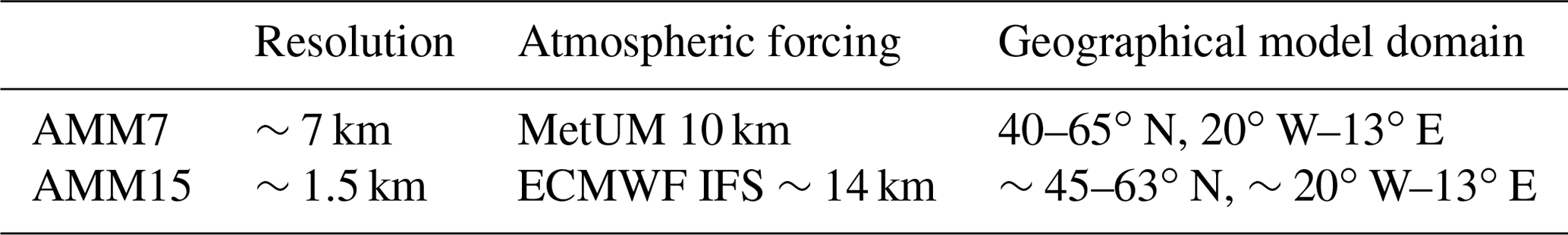
Table 2Details of equivalent neighbourhoods used when comparing AMM7 and AMM15.
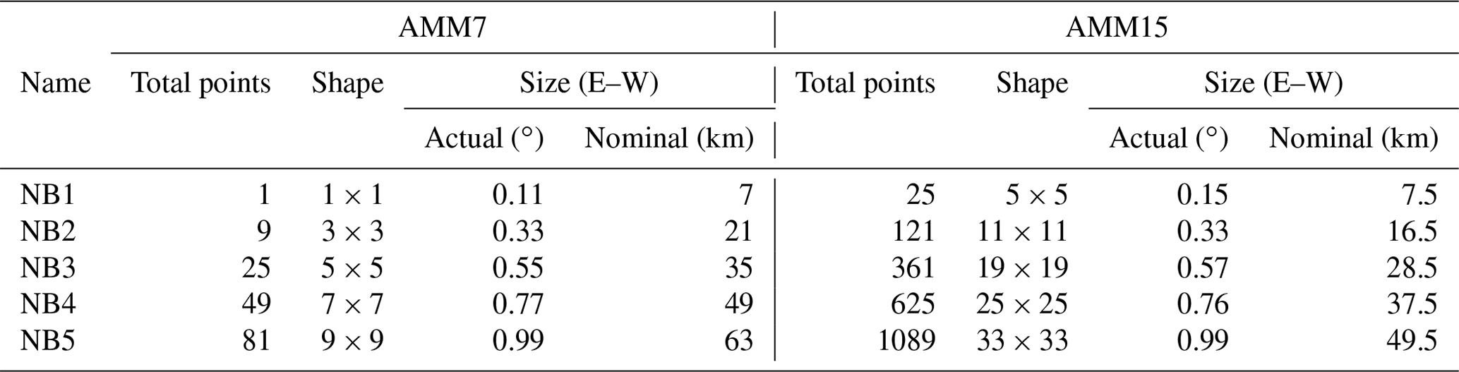
Additionally, the two model configurations do not have the same aspect ratio of grid points. AMM7 has a longitudinal resolution of ∼0.11∘ and a latitudinal resolution of ∼0.066∘ (a ratio of 3:5), whilst the AMM15 grid has a resolution of ∼0.03 and ∼0.0135∘, respectively (a ratio of 5:11). HiRA neighbourhoods typically contain the same number of grid points in the zonal and meridional directions which will lead to discrepancies in the area selected when comparing models with different grid aspect ratios, depending on whether the comparison is based on neighbourhoods with a similar longitudinal or similar latitudinal size. This difference will scale as the neighbourhood size increases, as shown in Fig. 4 and Table 2. The onus is therefore on the user to understand any difference in grid structure, and therefore within the HiRA neighbourhoods, between models being compared and to allow for this when comparing equivalent neighbourhoods.
For this study, we have matched neighbourhoods between model configurations based on their longitudinal size. The equivalent neighbourhoods used to show similar areas within the two configurations are indicated in Table 2 along with the bar style and naming convention used throughout.
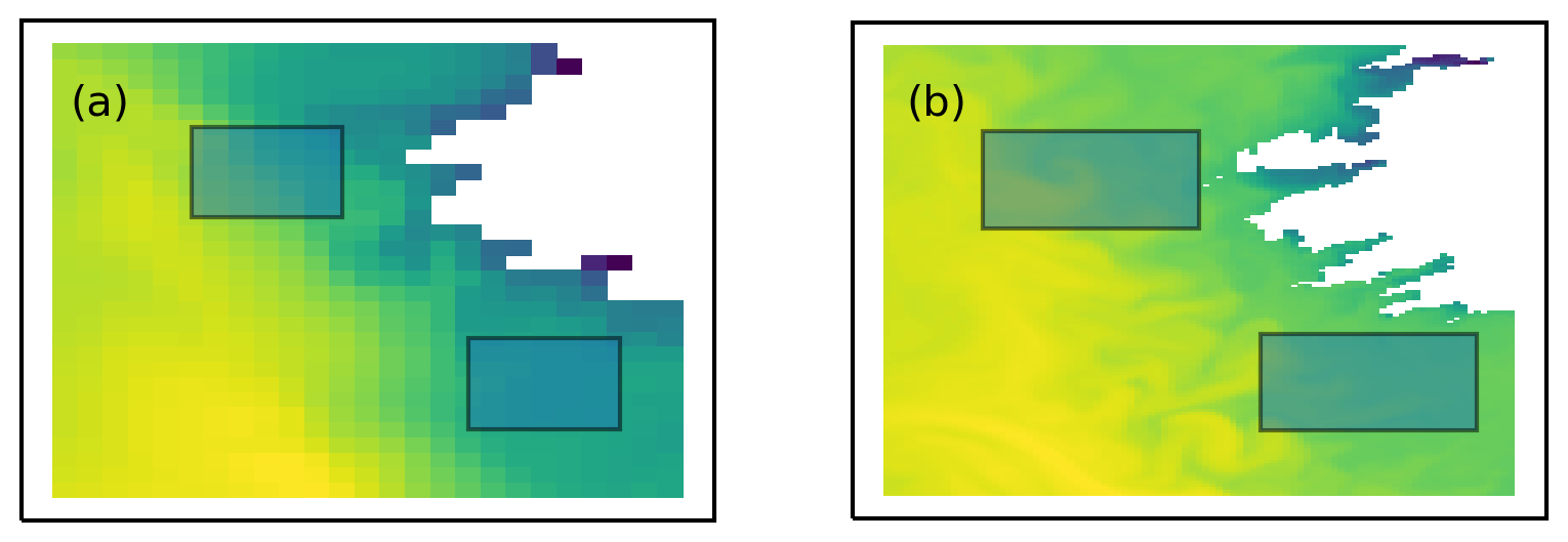
Figure 5Similar neighbourhood sizes for a 49 km neighbourhood using the approximate resolutions (7 and 1.5 km) with (a) AMM7 with a 7×7 neighbourhood and (b) AMM15 with a 33×33 neighbourhood. Whilst the neighbourhoods are similar sizes in the latitudinal direction, the AMM15 neighbourhood is sampling a much larger area due to different scales in the longitudinal direction. This means that a comparison with a 25×25 AMM15 neighbourhood is more appropriate.
For ocean applications, there are other aspects of the processing to be aware of when using neighbourhood methods. This is mainly related to the presence of coastlines and how their representation changes resolution (as defined by the land–sea mask) and the treatment of observations within HiRA neighbourhoods. Figure 5 illustrates the contrasting land–sea boundaries due to the different resolutions of the two configurations. When calculating HiRA neighbourhood values, all forecast values in the specific neighbourhood around an observation must be present for a score to be calculated. If any forecast points within a neighbourhood contain missing data, then that observation at that neighbourhood size is rejected. This is to ensure that the resolution of the “ensemble”, which is defined or determined by the number of members, remains the same. For typical atmospheric fields such as screen temperature, this is not an issue, but with parameters that have physical boundaries (coastlines), such as SST, there will be discontinuities in the forecast field that depend on the location of the land–sea boundary. For coastal observations, this means that as the neighbourhood size increases, it is more likely that an observation will be rejected from the comparison due to missing data. Even at the grid scale, the nearest model grid point to an observation may not be a sea point. In addition, different land–sea borders between models mean that potentially some observations will be rejected from one model comparison but will be retained in the other because of missing forecast points within their respective neighbourhoods. Care should be taken when implementing HiRA to check the observations available to each model configuration when assessing the results and make a judgement as to whether the differences are important.
There are potential ways to ensure equalisation, for example, only using observations that are available in both configurations for a location and neighbourhoods, or only observations away from the coast. For the purposes of this study, which aims to show the utility of the method, it was judged important to use as many observations as possible, so as to capture any potential pitfalls in the application of the framework, which would be relevant to any future application of it.

Figure 6Number of observation sites within NB1, NB3 and NB5 for AMM15 and AMM7. Numbers are those used during September 2019 but represent typical total observations during a month. Matching line styles represent equivalent neighbourhoods.
Figure 6 shows the number of observations available to each neighbourhood for each day during September 2019. For each model configuration, it shows how these observations vary within the HiRA framework. There are several reasons for the differences shown in the plot. There is the difference mentioned previously whereby a model neighbourhood includes a land point and therefore is rejected from the calculations because the number of quasi-ensemble members is no longer the same. This is more likely for coastal observations and depends on the particularities of the model land–sea mask near each observation. This rejection is more likely for the high-resolution AMM15 when looking at equivalent areas, in part due to the larger number of grid boxes being used; however, there are also instances of observations being rejected from the coarser-resolution AMM7 and not the higher-resolution AMM15 due to nuances of the land–sea mask.
It is apparent that for equivalent neighbourhoods there are typically more observations available for the coarser model configuration and that this difference is largest for the smallest equivalent neighbourhood size but becoming less obvious at larger neighbourhoods. It could therefore be worth considering that the large benefit in AMM15 when looking at the first equivalent neighbourhood is potentially influenced by the difference in observations. As the neighbourhood sizes increase, the number of observations reduces due to the higher likelihood of a land point being part of a larger neighbourhood. It is also noted that there is a general daily variability in the number of observations present, based on differences in the observations reporting on any particular day within the co-located domain.
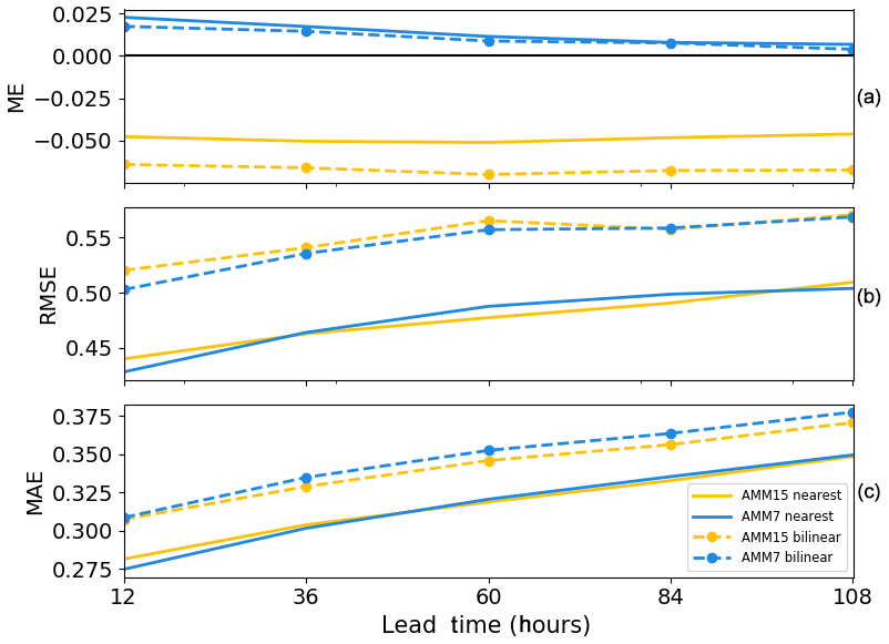
Figure 7Verification results using a typical statistics approach for January–September 2019. Mean error (a), root mean square error (b) and mean absolute error (c) results are shown for the two model configurations. Two methods of matching forecast to observations points have been used: a nearest-neighbour approach (solid) representing the single-grid-point results from HiRA and a bilinear interpolation approach (dashed) more typically used in operational ocean verification.
Figure 7 shows the aggregated results from the study period defined in Sect. 2 by applying typical verification statistics. Results have been averaged across the entire period from January to September and output relative to the forecast validity time. Two methods of matching forecast grid points to observation locations have been used. Bilinear interpolation is typically the approach used in traditional verification of SST, as it is a smoothly varying field. A nearest-neighbour approach has also been shown, as this is the method that would be used for HiRA when applying it at the grid scale.
It is noted that the two methods of matching forecasts to observation locations give quite different results. For the mean error, the impact of moving from a single-grid-point approach to a bilinear interpolation method appears to be minor for the AMM7 model but is more severe for AMM15, resulting in a larger error across all lead times. For the RMSE, the picture is more mixed, generally suggesting that the AMM7 forecasts are better when using a bilinear interpolation method but giving no clear overall steer when the nearest grid point is used. However, the impact of taking a bilinear approach results in much higher gross errors across all lead times when compared to the nearest grid point approach.
The MAE has been suggested as a more appropriate metric than the RMSE for ocean fields using (as is the case here) near-real-time observation data (Brassington, 2017). In Fig. 6, it can be seen that the nearest grid point approach for both AMM7 and AMM15 gives almost exactly the same results, except for the shortest of lead times. For the bilinear interpolation method, AMM15 has a smaller error than AMM7 as lead time increases, behaviour which is not apparent when RMSE is applied.
Based on the interpolated RMSE results in Fig. 6, it would be hard to conclude that there was a significant benefit to using high-resolution ocean models for forecasting SSTs. This is where the HiRA framework can be applied. It can be used to provide more information, which can better inform any conclusions on model error.
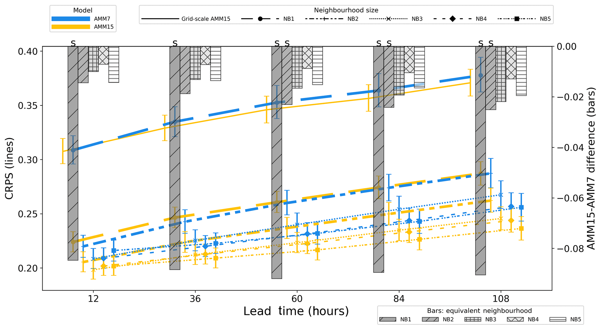
Figure 8Summary of CRPS (left axis, lines) and CRPS difference (right axis, bars) for the January 2019 to September 2019 period for AMM7 and AMM15 models at different neighbourhood sizes. Error bars represent 95 % confidence intervals generated using a bootstrap with replacement method for 10 000 samples. An “S” above the bar denotes that 95 % error bars for the two models do not overlap.
Figure 8 shows the results for AMM7 and AMM15 for the January–September 2019 period using the HiRA framework with the CRPS. The lines on the plot show the CRPS for the two model configurations for different neighbourhood sizes, each plotted against lead time. Similar line styles are used to represent equivalent neighbourhood sizes. Confidence intervals have been generated by applying a bootstrap with replacement method, using 10 000 samples, to the domain-averaged CRPS (e.g. Efron and Tibshirani, 1986). The error bars represent the 95 % confidence level. The results for the single grid point show the MAE and are the same as would be obtained using a traditional (precise) matching. In the case of CRPS, where a lower score is better, we see that AMM15 is better than AMM7, though not significantly so, except at shorter lead times where there is little difference.
The differences at equivalent neighbourhood sizes are displayed as a bar plot on the same figure, with scores referenced with respect to the right-hand axis. Line markers and error bars have been offset to aid visualisation, such that results for equivalent neighbourhoods are displayed in the same vertical column as the difference indicated by the bar plot. The details of the equivalent neighbourhood sizes are presented in Table 2. Since a lower CRPS score is better, a positively orientated (upwards) bar implies AMM7 is better, whilst a negatively orientated (downwards) bar means AMM15 is better.
As indicated in Table 2, NB1 compares the single-grid-point results of AMM7 with a 25-member pseudo-ensemble constructed from a 5×5 AMM15 neighbourhood. Given the different resolutions of the two configurations, these two neighbourhoods represent similar physical areas from each model domain, with AMM7 only represented by a single forecast value for each observation but AMM15 represented by 25 values covering the same area, and as such potentially better able to represent small-scale variability within that area.
At this equivalent scale, the AMM15 results are markedly better than AMM7, with lower errors, suggesting that overall the AMM15 neighbourhood better represents the variation around the observation than the coarser single grid point of AMM7. In the next set of equivalent neighbourhoods (NB2), the gap between the two configurations has closed, but AMM15 is still consistently better than AMM7 as lead time increases. Above this scale, the neighbourhood values tend towards similarity and then start to diverge again suggesting that the representative scale of the neighbourhoods has been reached and that errors are essentially random.
Whilst the overall HiRA neighbourhood results for the co-located domains appear to show a benefit to using a higher-resolution model forecast, it could be that these results are influenced by the spatial distribution of observations within the domain and the characteristics of the forecasts at those locations. In order to investigate whether this was important behaviour, the results were separated into two domains: one representing the continental shelf part of the domain (where the bathymetry <200 m) and the other representing the deeper, off-shelf, ocean component (Fig. 9). HiRA results were compared for observations only within each masked domain.
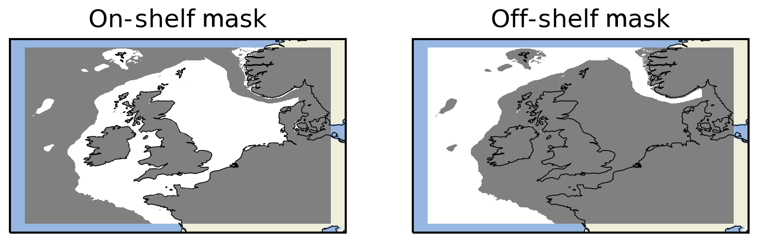
Figure 9On-shelf and off-shelf masking regions within the co-located AMM7 and AMM15 domain (data within the grey areas are masked).

Figure 10Summary of on-shelf CRPS (left axis, lines) and CRPS difference (right axis, bars) for the January 2019 to September 2019 period for AMM7 and AMM15 models at different neighbourhood sizes. Error bars represent 95 % confidence values obtained from 10 000 samples using bootstrap with replacement. An “S” above the bar denotes that 95 % error bars for the two models do not overlap.
On-shelf results (Fig. 10) show that at the grid scale the results for both AMM7 and AMM15 are worse for this subdomain. This could be explained by both the complexity of processes (tides, friction, river mixing, topographical effects, etc.) and the small dynamical scales associated with shallow waters on the shelf (Holt et al., 2017).
The on-shelf spatial variability in SST across a neighbourhood is likely to be higher than for an equivalent deep ocean neighbourhood due to small-scale changes in bathymetry and, for some observations, the impact of coastal effects. Both AMM7 and AMM15 show improvement in CRPS with increased neighbourhood size until the CRPS plateaus in the range 0.225 to 0.25, with AMM15 generally better than AMM7 for equivalent neighbourhood sizes. Scores get worse (errors increase) for both model configurations as the forecast lead time increases.
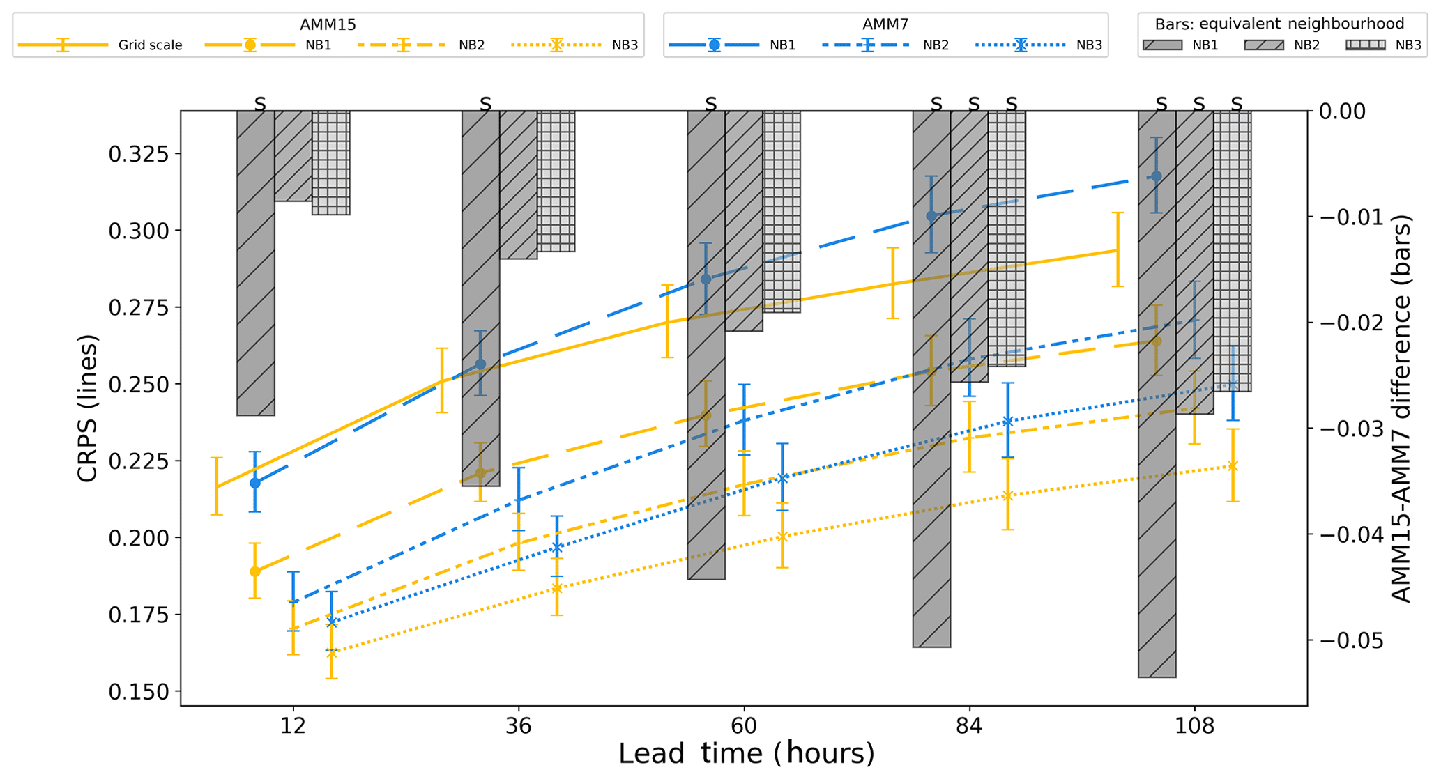
Figure 11Summary of off-shelf CRPS (left axis, lines) and CRPS difference (right axis, bars) for the January 2019 to September 2019 period for AMM7 and AMM15 models at different neighbourhood sizes. Error bars represent 95 % confidence values obtained from 10 000 samples using bootstrap with replacement. An “S” above the bar denotes that 95 % error bars for the two models do not overlap.
For off-shelf results (Fig. 11), CRPS is much better (smaller error) at both the grid scale and for HiRA neighbourhoods, suggesting that both configurations are better at forecasting these deep ocean SSTs (or that it is easier to do so). There is still an improvement in CRPS when going from the grid scale (single grid box) to neighbourhoods, but the value of that change is much smaller than that for the on-shelf subdomain. When comparing equivalent neighbourhoods, AMM15 still gives consistently better results (smaller errors) and appears to improve over AMM7 as lead time increases in contrast to the on-shelf results.
It is likely that the neighbourhood at which we lose representativity will be larger for the deeper ocean than the shelf area because of the larger scale of dynamical processes in deep water. When choosing an optimum neighbourhood to use for assessment, care should be taken to check whether there are different representativity levels in the data (such as here for on-shelf and off-shelf) and pragmatically choose the smaller of those equivalent neighbourhoods when looking at data combining the different representativity levels.
Overall, for the January–September 2019 period, AMM15 demonstrates a lower (better) CRPS than AMM7 when looking at the HiRA neighbourhoods. However, this also appears to be true at the grid scale over the assessment period. One of the aspects that HiRA is trying to provide additional information about is whether higher-resolution models can demonstrate improvement over coarser models against a perception that the coarser models score better in standard verification forecast assessments. Assessed over the whole period, this initial premise does not appear to hold true; therefore, a deeper look at the data is required to assess whether this signal is consistent within shorter time periods or if there are underlying periods contributing significant and contrasting results to the whole-period aggregate.
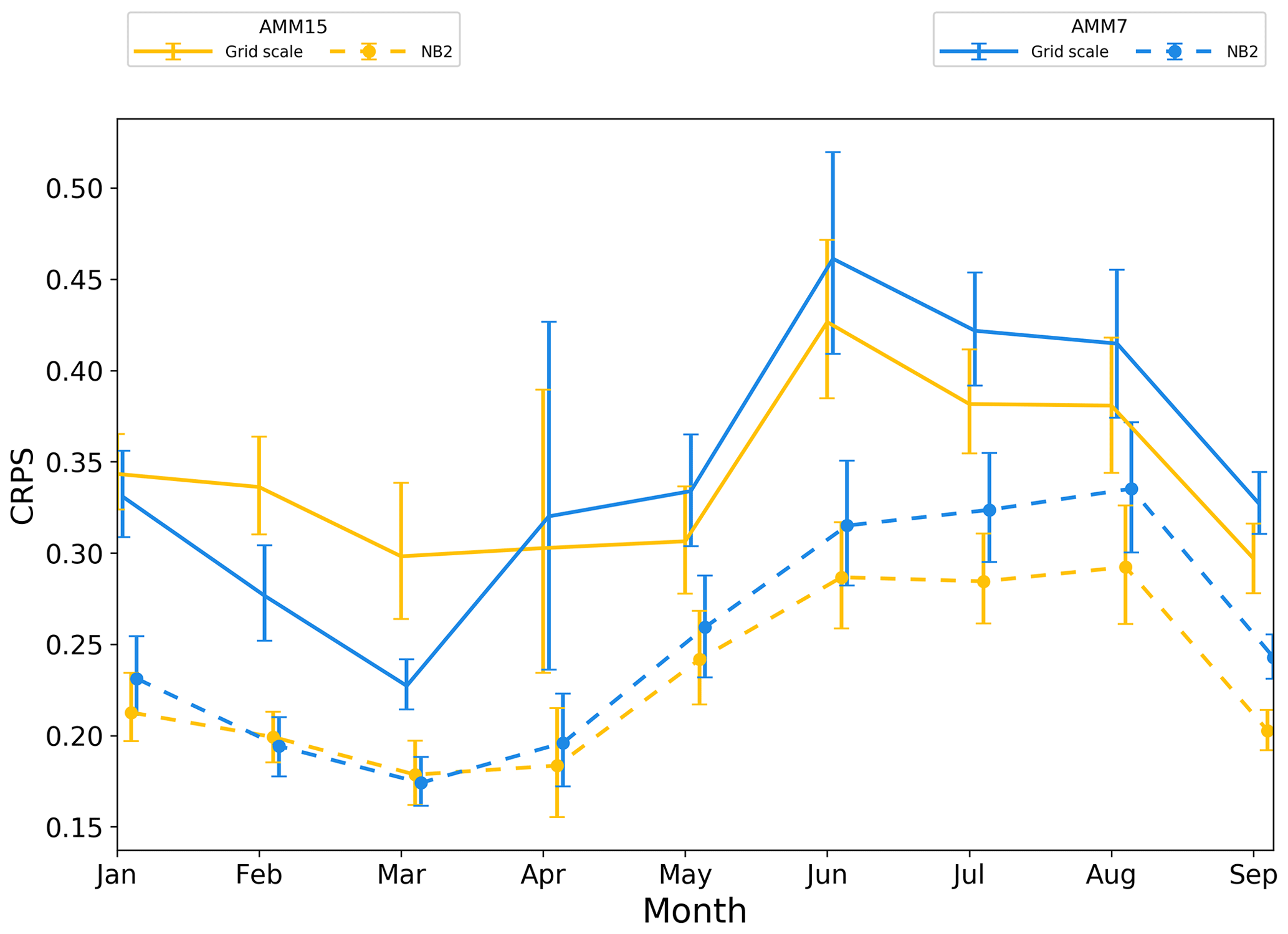
Figure 12Monthly time series of whole-domain CRPS scores for the grid scale (solid line) and NB2 neighbourhood (dashes) for T+60 forecasts. Error bars represent 95 % confidence values obtained from 10 000 samples using bootstrap with replacement. Error bars have been staggered in the x direction to aid clarity.
Figure 12 shows a monthly breakdown of the grid scale and the NB2 HiRA neighbourhood scores at T+60. This shows the underlying monthly variability not immediately apparent in the whole-period plots. Notably for the January to March period, AMM7 outperforms AMM15 at the grid scale. With the introduction of HiRA neighbourhoods, AMM7 still performs better for February and March but the difference between the models is significantly reduced. For these monthly time series, the error bars increase in size relative to the summary plots (e.g. Fig. 8) due to the reduction in data available. The sample size will have an impact on the error bars as the smaller the sample, the less representative of the true population the data are likely to be. April in particular contained several days of missing forecast data, leading to a reduction in sample size and corresponding increase in error bar size, whilst during May there was a period with reduced numbers of observations.
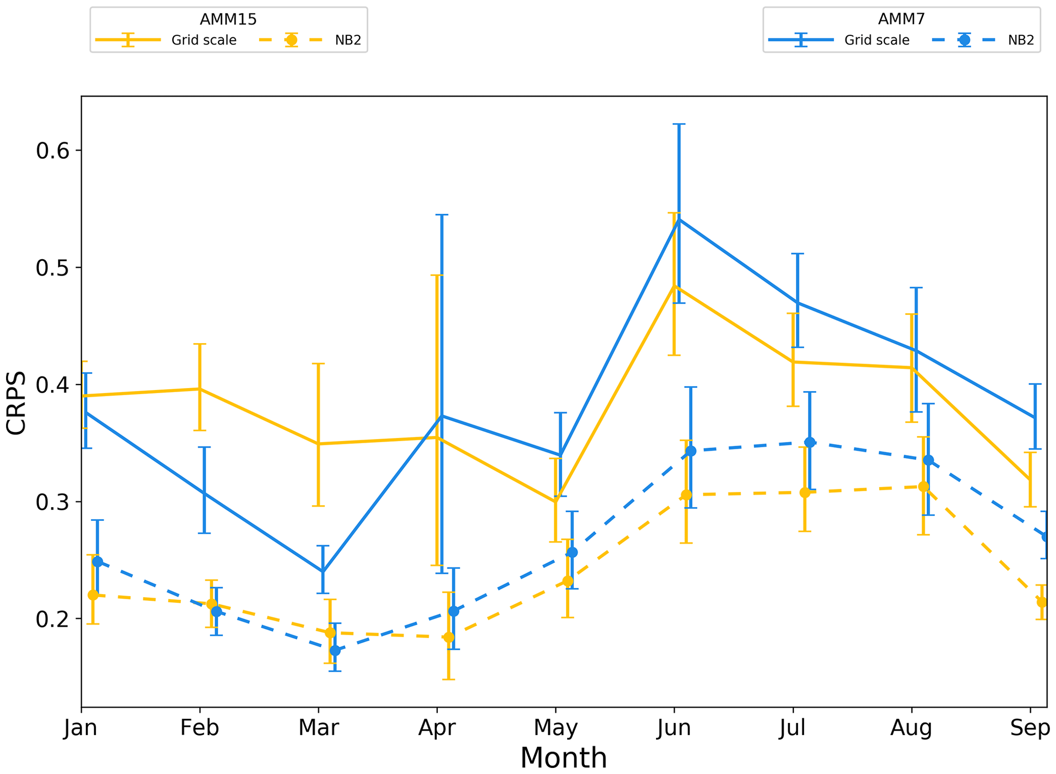
Figure 13On-shelf monthly time series of CRPS. Error bars represent 95 % confidence values obtained from 10 000 samples using bootstrap with replacement.
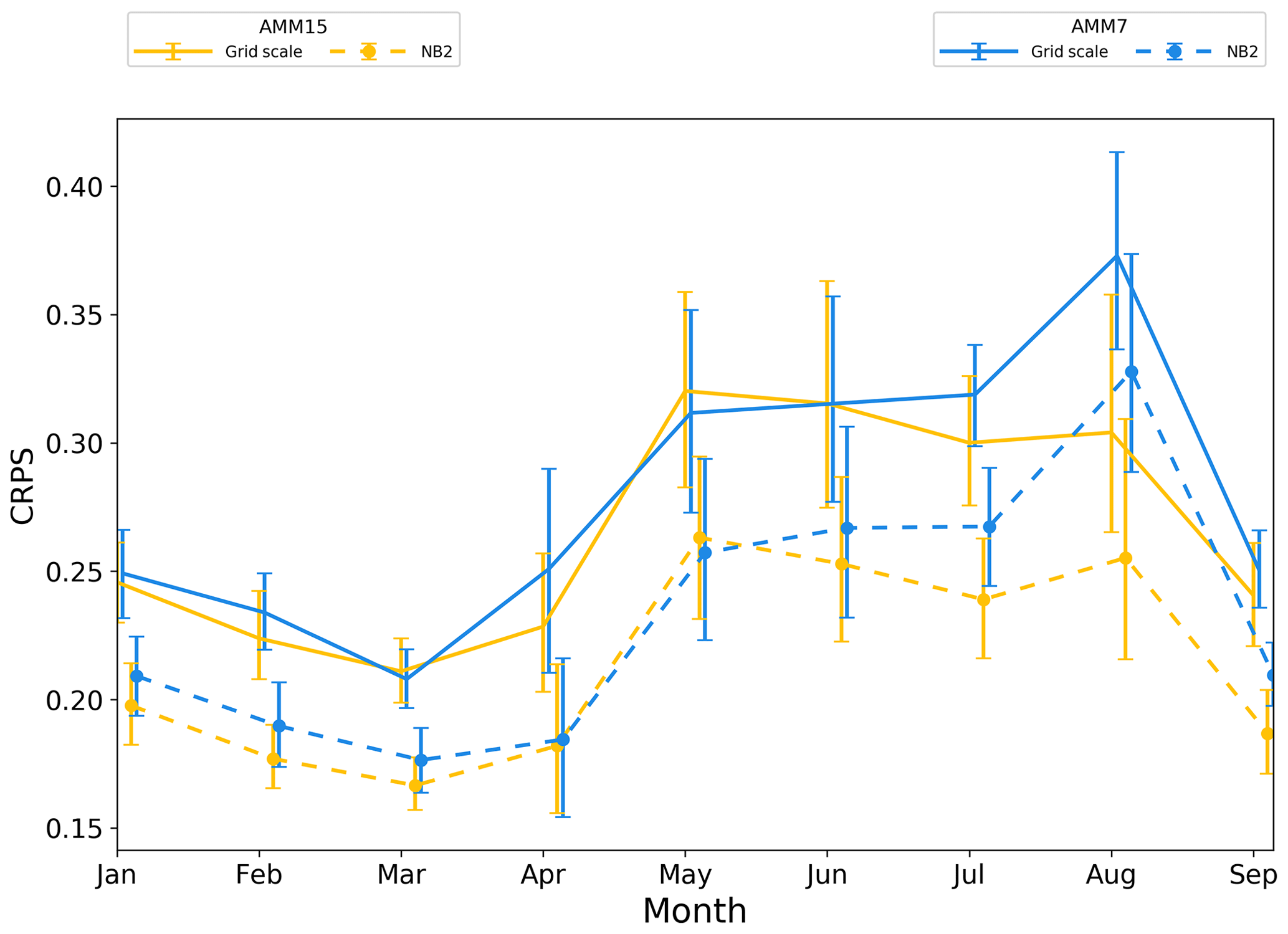
Figure 14Off-shelf monthly time series of CRPS. Error bars represent 95 % confidence values obtained from 10 000 samples using bootstrap with replacement.
The same pattern is present for the on-shelf subdomain (Fig. 13), where what appears to be a significant benefit for AMM7 during February and March is less clear-cut at the NB2 neighbourhood. For the off-shelf subdomain (Fig. 14), differences between the two configurations at the grid scale are mainly apparent during the summer months. At the NB2 scale, AMM15 potentially demonstrates more benefit than AMM7 except for April and May, where the two show similar results. There is a balance to be struck in this conclusion as the differences between the two models are rarely greater than the 95 % error bars. This in itself does not mean that the results are not significant. However, care should be taken when interpreting such a result as a statistical conclusion rather than broad guidance as to model performance. Attempts to reduce the error bar size, such as increasing the number of observations or number of times within the period, would aid this interpretation.
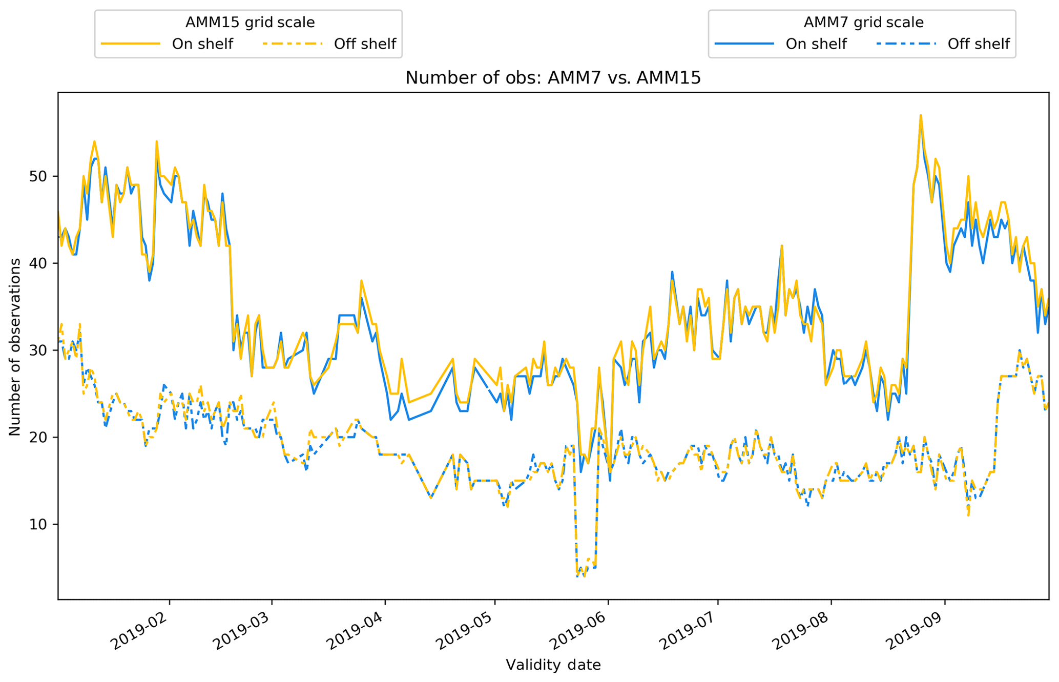
One noticeable aspect of the time series plots is that the whole-domain plot is heavily influenced by the on-shelf results. This is due to the difference in observation numbers as shown in Fig. 15, with the on-shelf domain having more observations overall, sometimes significantly more, for example, during January or mid-to-late August. For the overall domain, the on-shelf observations will contribute more to the overall score, and hence the underlying off-shelf signal will tend to be masked. This is an indication of why verification is more useful when done over smaller, more homogeneous subregions, rather than verifying everything together, with the caveat that sample sizes are large enough, since underlying signals can be swamped by dominant error types.
In this study, the HiRA framework has been applied to SST forecasts from two ocean models with different resolutions. This enables a different view of the forecast errors than obtained using traditional (precise) grid-scale matching against ocean observations. Particularly, it enables us to demonstrate the additional value of high-resolution model. When considered more appropriately, high-resolution models (with the ability to forecast small-scale detail) have lower errors when compared to the smoother forecasts provided by a coarser-resolution model.
The HiRA framework was intended to address the question of whether moving to higher resolution adds value. This study has identified and highlighted aspects that need to be considered when setting up such an assessment. Prior to this study, routine verification statistics typically showed that coarser-resolution models had equivalent skill to or more skill than higher-resolution models (e.g. Mass et al., 2002; Tonani et al., 2019). During the January to September 2019 period, grid-scale verification within this assessment showed that the coarser-resolution AMM7 often demonstrated lower errors than AMM15.
HiRA neighbourhoods were applied and the data then assessed using the CRPS, showing a large reduction (improvement) in errors for AMM15 when going from a grid-scale, point-based verification assessment to a neighbourhood, ensemble approach. When applying an equivalent-sized neighbourhood to both configurations, AMM15 typically demonstrated lower (better) scores. These scores were in turn broken down into off-shelf and on-shelf subdomains and showed that the different physical processes in these areas affected the results. Forecast verification studies tailored for the coastal/shelf areas are needed to properly understand the forecast skills in areas with high complexity and fast-evolving dynamics.
When constructing HiRA neighbourhoods, the spatial scales that are appropriate for the parameter must be considered carefully. This often means running at several neighbourhood sizes and determining where the scores no longer seem physically representative. When comparing models, care should be taken to construct neighbourhood sizes that are similarly sized spatially; the details of the neighbourhood sizes will depend on the structure and resolution of the model grid.
Treatment of observations is also important in any verification setup. For this study, the fact that there are different numbers of observations present at each neighbourhood scale (as observations are rejected due to land contamination) means that there is never an optimally equalised dataset (i.e. the same observations for all models and for all neighbourhood sizes). It also means that comparison of the different neighbourhood results from a single model is ill advised, in this case, as the observations numbers can be very different, and therefore the model forecast is being sampled at different locations. Despite this, observation numbers should be similar when looking at matched spatially sized neighbourhoods from different models if results are to be compared. One of the main constraints identified through this work is both the sparsity and geographical distribution of observations throughout the NWS domain, with several viable locations rejected during the HiRA processing due to their proximity to coastlines.
The purest assessment, in terms of observations, would involve a fixed set of observations, equalised across both model configurations and all neighbourhoods at every time. This would remove the variation in observation numbers seen as neighbourhood sizes increase as well as those seen between the two models and give a clean comparison between two models.
Care should be taken when applying strict equalisation rules, as this could result in only a small number of observations being used. The total number of observations used should be large enough to ensure that the sample is large enough to produce robust results and satisfy rules for statistical significance. Equalisation rules could also unfairly affect the spatial sampling of the verification domain. For example, in this study, coastal observations would be affected more than deep ocean observations if neighbourhood equalisation were applied, due to the proximity of the coast.
To a lesser extent, the variation in observation numbers on a day-to-day timescale also has an impact on any results and could mean that incorrect importance is attributed to certain results, which are simply due to fluctuations in observation numbers.
The fact that the errors can be reduced through the use of neighbourhoods shows that the ocean and the atmosphere have similarities in the way the forecasts behave as a function of resolution. This study did not consider the concept of skill, which incorporates the performance of the forecast relative to a pre-defined benchmark. For the ocean, the choice of reference needs to be considered. This could be the subject of further work.
To our knowledge, this work is the first attempt to use neighbourhood techniques to assess ocean models. The promising results showing reductions in errors of the finer-resolution configuration warrant further work. We see a number of directions the current study could be extended.
The study was conducted on daily output which should be appropriate to address eddy mesoscale variability, but observations are distributed at hourly resolution, and so the next logical step would be to assess the hourly forecasts against the hourly observation and see how this impacted the results. This will increase the sample size, if all hourly observations were considered together. However, it is impossible to speculate on whether considering hourly forecasts would lead to more noisy statistics, counteracting the larger sample size.
This assessment only looked at SST for this initial examination. Consideration of other ocean variables would also be of interest, including looking at derived diagnostics such as mixed layer depth, but the sparsity of observations available for some variables may limit the case studies available. HiRA as a framework is not remaining static. Enhancements to introduce non-regular flow-dependent neighbourhoods are planned and may be of benefit to ocean applications in the future. Finally, an advantage of using the HiRA framework is that results obtained from deterministic ocean models could also be compared against results from ensemble models when these become available for ocean applications.
Data used in this paper was downloaded from the Copernicus Marine and Environment Monitoring Service (CMEMS).
The datasets used were https://resources.marine.copernicus.eu/?option=com_csw&task=results?option=com_csw&view=details&product_id=NORTHWESTSHELF_ANALYSIS_FORECAST_PHYS_004_001_b (last access: October 2019), https://resources.marine.copernicus.eu/?option=com_csw&task=results?option=com_csw&view=details&product_id=NORTHWESTSHELF_ANALYSIS_FORECAST_PHY_004_013 (last access: October 2019) and https://resources.marine.copernicus.eu/?option=com_csw&task=results?option=com_csw&view=details&product_id=INSITU_NWS_NRT_OBSERVATIONS_013_036 (last access: October 2019).
All authors contributed to the introduction, data and methods, and conclusions. RC, JM and MM contributed to the scientific evaluation and analysis of the results. RC and JM designed and ran the model assessments. CP supported the assessments through the provision and reformatting of the data used. MT provided details on the model configurations used.
The authors declare that they have no conflict of interest.
This study has been conducted using EU Copernicus Marine Service Information.
This work has been carried out as part of the Copernicus Marine Environment Monitoring Service (CMEMS) HiVE project. CMEMS is implemented by Mercator Ocean International in the framework of a delegation agreement with the European Union.
Model Evaluation Tools (MET) was developed at the National Center for Atmospheric Research (NCAR) through grants from the National Science Foundation (NSF), the National Oceanic and Atmospheric Administration (NOAA), the United States Air Force (USAF) and the United States Department of Energy (DOE). NCAR is sponsored by the United States National Science Foundation.
This paper was edited by Anna Rubio and reviewed by two anonymous referees.
Aznar, R., Sotillo, M., Cailleau, S., Lorente, P., Levier, B., Amo-Baladrón, A., Reffray, G., and Alvarez Fanjul, E.: Strengths and weaknesses of the CMEMS forecasted and reanalyzed solutions for the Iberia-Biscay-Ireland (IBI) waters, J. Marine. Syst., 159, 1–14, https://doi.org/10.1016/j.jmarsys.2016.02.007, 2016.
Brassington, G.: Forecast Errors, Goodness, and Verification in Ocean Forecasting, J. Marine Res., 75, 403–433, https://doi.org/10.1357/002224017821836851, 2017.
Brier, G. W.: Verification of Forecasts Expressed in Terms of Probability, Mon. Weather Rev., 78, 1–3, https://doi.org/10.1175/1520-0493(1950)078<0001:VOFEIT>2.0.CO;2, 1950.
Brown, T. A.: Admissible scoring systems for continuous distributions, Santa Monica, CA, RAND Corporation, available at: https://www.rand.org/pubs/papers/P5235.html (last access: March 2020), 1974.
Casati, B., Ross, G., and Stephenson, D. B.: A new intensity-scale approach for the verification of spatial precipitation forecasts, Met. Apps., 11, 141–154, https://doi.org/10.1017/S1350482704001239, 2004.
Davis, C., Brown, B., and Bullock, R.: Object-Based Verification of Precipitation Forecasts. Part I: Methodology and Application to Mesoscale Rain Areas, Mon. Weather Rev., 134, 1772–1784, https://doi.org/10.1175/MWR3145.1, 2006.
Dorninger, M., Gilleland, E., Casati, B., Mittermaier, M. P., Ebert, E. E., Brown, B. G., and Wilson, L. J.: The Setup of the MesoVICT Project, B. Am. Meteorol. Soc., 99, 1887–1906, https://doi.org/10.1175/BAMS-D-17-0164.1, 2018.
Ebert, E. E.: Fuzzy verification of high-resolution gridded forecasts: a review and proposed framework, Met. Apps, 15, 51–64, https://doi.org/10.1002/met.25, 2008.
Efron, B. and Tibshirani, R.: Bootstrap methods for standard errors, confidence intervals, and other measures of statistical accuracy, Stat. Sci., 1, 54–77, 1986.
Epstein, E. S.: A Scoring System for Probability Forecasts of Ranked Categories, J. Appl. Meteorol., 8, 985–987, 1969.
Gilleland, E., Ahijevych, D., Brown, B. G., Casati, B., and Ebert, E. E.: Intercomparison of Spatial Forecast Verification Methods, Weather Forecast., 24, 1416–1430, https://doi.org/10.1175/2009WAF2222269.1, 2009.
Goessling, H. F., Tietsche, S., Day, J. J., Hawkins, E., and Jung, T. : Predictability of the Arctic sea ice edge, Geophys. Res. Lett., 43, 1642–1650, https://doi.org/10.1002/2015GL067232, 2016.
Graham, J. A., O'Dea, E., Holt, J., Polton, J., Hewitt, H. T., Furner, R., Guihou, K., Brereton, A., Arnold, A., Wakelin, S., Castillo Sanchez, J. M., and Mayorga Adame, C. G.: AMM15: a new high-resolution NEMO configuration for operational simulation of the European north-west shelf, Geosci. Model Dev., 11, 681–696, https://doi.org/10.5194/gmd-11-681-2018, 2018.
Hernandez, F., Blockley, E., Brassington, G. B., Davidson, F., Divakaran, P., Drévillon, M., Ishizaki, S., Garcia-Sotillo, M., Hogan, P. J., Lagemaa, P., Levier, B., Martin, M., Mehra, A., Mooers, C., Ferry, N., Ryan, A., Regnier, C., Sellar, A., Smith, G. C., Sofianos, S., Spindler, T., Volpe, G., Wilkin, J., Zaron, E. D., and Zhang, A.: Recent progress in performance evaluations and near real-time assessment of operational ocean products, J. Oper. Oceanogr., 8, 221–238, https://doi.org/10.1080/1755876X.2015.1050282, 2015.
Hernandez, F., Smith, G., Baetens, K., Cossarini, G., Garcia-Hermosa, I., Drevillon, M., Maksymczuk, J., Melet, A., Regnier, C., and von Schuckmann, K.: Measuring Performances, Skill and Accuracy in Operational Oceanography: New Challenges and Approaches, in: New Frontiers in Operational Oceanography, edited by: Chassignet, E., Pascual, A., Tintore, J., and Verron, J., GODAE OceanView, 759–796, https://doi.org/10.17125/gov2018.ch29, 2018.
Hersbach, H.: Decomposition of the Continuous Ranked Probability Score for Ensemble Prediction Systems, Weather Forecast., 15, 559–570, https://doi.org/10.1175/1520-0434(2000)015<0559:DOTCRP>2.0.CO;2, 2000.
Holt, J., Hyder, P., Ashworth, M., Harle, J., Hewitt, H. T., Liu, H., New, A. L., Pickles, S., Porter, A., Popova, E., Allen, J. I., Siddorn, J., and Wood, R.: Prospects for improving the representation of coastal and shelf seas in global ocean models, Geosci. Model Dev., 10, 499–523, https://doi.org/10.5194/gmd-10-499-2017, 2017.
Howarth, M. and Pugh, D.: Chapter 4 Observations of Tides Over the Continental Shelf of North-West Europe, Elsevier Oceanography Series, 35, 135–188, https://doi.org/10.1016/S0422-9894(08)70502-6, 1983.
Juza, M., Mourre, B., Lellouche, J. M., Tonani M., and Tintoré, J.: From basin to sub-basin scale assessment and intercomparison of numerical simulations in the western Mediterranean Sea, J. Mar. Syst., 149, 36–49, https://doi.org/10.1016/j.jmarsys.2015.04.010, 2015.
Keil, C. and Craig, G. C.: A Displacement-Based Error Measure Applied in a Regional Ensemble Forecasting System, Mon. Weather Rev., 135, 3248–3259, https://doi.org/10.1175/MWR3457.1, 2007.
King, R., While, J., Martin, M. J., Lea, D. J., Lemieux-Dudon, B., Waters, J., and O'Dea, E.: Improving the initialisation of the Met Office operational shelf-seas model, Ocean Model., 130, 1–14, 2018.
Le Traon, P. Y., Reppucci, A., Alvarez Fanjul, E., Aouf, L., Behrens, A., Belmonte, M., Bentamy, A., Bertino, L., Brando, V. E., Kreiner, M. B., Benkiran, M., Carval, T., Ciliberti, S. A., Claustre, H., Clementi, E., Coppini, G., Cossarini, G., De Alfonso Alonso-Muñoyerro, M., Delamarche, A., Dibarboure, G., Dinessen, F., Drevillon, M., Drillet, Y., Faugere, Y., Fernández, V., Fleming, A., Garcia-Hermosa, M. I., Sotillo, M. G., Garric, G., Gasparin, F., Giordan, C., Gehlen, M., Gregoire, M. L., Guinehut, S., Hamon, M., Harris, C., Hernandez, F., Hinkler, J. B., Hoyer, J., Karvonen, J., Kay, S., King, R., Lavergne, T., Lemieux-Dudon, B., Lima, L., Mao, C., Martin, M. J., Masina, S., Melet, A., Buongiorno Nardelli, B., Nolan, G., Pascual, A., Pistoia, J., Palazov, A., Piolle, J. F., Pujol, M. I., Pequignet, A. C., Peneva, E., Pérez Gómez, B., Petit de la Villeon, L., Pinardi, N., Pisano, A., Pouliquen, S., Reid, R., Remy, E., Santoleri, R., Siddorn, J., She, J., Staneva, J., Stoffelen, A., Tonani, M., Vandenbulcke, L., von Schuckmann, K., Volpe, G., Wettre, C., and Zacharioudaki, A.: From Observation to Information and Users: The Copernicus Marine Service Perspective, Front. Mar. Sci., 6, 234, https://doi.org/10.3389/fmars.2019.00234, 2019.
Lorente, P., García-Sotillo, M., Amo-Baladrón, A., Aznar, R., Levier, B., Sánchez-Garrido, J. C., Sammartino, S., de Pascual-Collar, Á., Reffray, G., Toledano, C., and Álvarez-Fanjul, E.: Skill assessment of global, regional, and coastal circulation forecast models: evaluating the benefits of dynamical downscaling in IBI (Iberia–Biscay–Ireland) surface waters, Ocean Sci., 15, 967–996, https://doi.org/10.5194/os-15-967-2019, 2019a.
Lorente, P., Sotillo, M., Amo-Baladrón, A., Aznar, R., Levier, B., Aouf, L., Dabrowski, T., Pascual, Á., Reffray, G., Dalphinet, A., Toledano Lozano, C., Rainaud, R., and Alvarez Fanjul, E. : The NARVAL Software Toolbox in Support of Ocean Models Skill Assessment at Regional and Coastal Scales, doi10.1007/978-3-030-22747-0_25, 2019b.
Madec, G. and the NEMO team: NEMO ocean engine, Note du Pôle de modélisation, Institut Pierre-Simon Laplace (IPSL), France, No 27 ISSN 1288-1619, 2016.
Mason, E., Ruiz, S., Bourdalle-Badie, R., Reffray, G., García-Sotillo, M., and Pascual, A.: New insight into 3-D mesoscale eddy properties from CMEMS operational models in the western Mediterranean, Ocean Sci., 15, 1111–1131, https://doi.org/10.5194/os-15-1111-2019, 2019.
Mass, C. F., Ovens, D., Westrick, K., and Colle, B. A.: DOES INCREASING HORIZONTAL RESOLUTION PRODUCE MORE SKILLFUL FORECASTS?, B. Am. Meteorol. Soc., 83, 407–430, https://doi.org/10.1175/1520-0477(2002)083<0407:DIHRPM>2.3.CO;2, 2002.
Mirouze, I., Blockley, E. W., Lea, D. J., Martin, M. J., and Bell, M. J.: A multiple length scale correlation operator for ocean data assimilation, Tellus A, 68, 29744, https://doi.org/10.3402/tellusa.v68.29744, 2016.
Mittermaier, M., Roberts, N., and Thompson, S. A.: A long-term assessment of precipitation forecast skill using the Fractions Skill Score, Met. Apps, 20, 176–186, https://doi.org/10.1002/met.296, 2013.
Mittermaier, M. P.: A Strategy for Verifying Near-Convection-Resolving Model Forecasts at Observing Sites, Weather Forecast., 29, 185–204, https://doi.org/10.1175/WAF-D-12-00075.1, 2014.
Mittermaier, M. P. and Csima, G.: Ensemble versus Deterministic Performance at the Kilometer Scale, Weather Forecast., 32, 1697–1709, https://doi.org/10.1175/WAF-D-16-0164.1, 2017.
Mogensen, K., Balmaseda, M. A., and Weaver, A.: The NEMOVAR ocean data assimilation system as implemented in the ECMWF ocean analysis for System 4, European Centre for Medium-Range Weather Forecasts, Reading, UK, 2012.
Mourre, B., Aguiar, E., Juza, M., Hernandez-Lasheras, J., Reyes, E., Heslop, E., Escudier, R., Cutolo, E., Ruiz, S., Mason, E., Pascual, A., and Tintoré, J.: Assessment of high-resolution regional ocean prediction systems using muli-platform observations: illustrations in the Western Mediterranean Sea, in: New Frontiers in Operational Oceanography, edited by: Chassignet, E., Pascual, A., Tintoré, J., and Verron, J., GODAE Ocean View, 663–694, https://doi.org/10.17125/gov2018.ch24, 2018.
O'Dea, E. J., Arnold, A. K., Edwards, K. P., Furner, R., Hyder, P., Martin, M. J., Siddorn, J. R., Storkey, D., While, J., Holt, J. T., and Liu, H.: An operational ocean forecast system incorporating NEMO and SST data assimilation for the tidally driven European North-West shelf, J. Oper. Oceanogr., 5, 3–17, https://doi.org/10.1080/1755876X.2012.11020128, 2012.
O'Dea, E., Furner, R., Wakelin, S., Siddorn, J., While, J., Sykes, P., King, R., Holt, J., and Hewitt, H.: The CO5 configuration of the 7 km Atlantic Margin Model: large-scale biases and sensitivity to forcing, physics options and vertical resolution, Geosci. Model Dev., 10, 2947–2969, https://doi.org/10.5194/gmd-10-2947-2017, 2017.
Rossa, A., Nurmi, P., and Ebert, E.: Overview of methods for the verification of quantitative precipitation forecasts, in: Precipitation: Advances in Measurement, Estimation and Prediction, edited by: Michaelides, S., Springer, Berlin, Heidelberg, 419–452, https://doi.org/10.1007/978-3-540-77655-0_16, 2008.
Tonani, M., Sykes, P., King, R. R., McConnell, N., Péquignet, A.-C., O'Dea, E., Graham, J. A., Polton, J., and Siddorn, J.: The impact of a new high-resolution ocean model on the Met Office North-West European Shelf forecasting system, Ocean Sci., 15, 1133–1158, https://doi.org/10.5194/os-15-1133-2019, 2019.
World Meteorological Organisation: Guide to Meteorological Instruments and Methods of Observation (WMO-No. 8, the CIMO Guide), available at: https://library.wmo.int/opac/doc_num.php?explnum_id=4147 (last access: June 2019), 2017.