the Creative Commons Attribution 4.0 License.
the Creative Commons Attribution 4.0 License.
 | 14 May 2020
Spatiotemporal variability of light attenuation and net ecosystem metabolism in a back-barrier estuary
Jeremy M. Testa
Steven E. Suttles
Alfredo L. Aretxabaleta
Quantifying system-wide biogeochemical dynamics and ecosystem metabolism in estuaries is often attempted using a long-term continuous record at a single site or short-term records at multiple sites due to sampling limitations that preclude long-term monitoring. However, differences in the dominant primary producer at a given location (e.g., phytoplankton versus benthic producers) control diel variations in dissolved oxygen and associated ecosystem metabolism, and they may confound metabolic estimates that do not account for this variability. We hypothesize that even in shallow, well-mixed estuaries there is strong spatiotemporal variability in ecosystem metabolism due to benthic and water-column properties, as well as ensuing feedbacks to sediment resuspension, light attenuation, and primary production. We tested this hypothesis by measuring hydrodynamic properties, biogeochemical variables (fluorescent dissolved organic matter – fDOM, turbidity, chlorophyll a fluorescence, dissolved oxygen), and photosynthetically active radiation (PAR) over 1 year at 15 min intervals at paired channel (unvegetated) and shoal (vegetated by eelgrass) sites in Chincoteague Bay, Maryland–Virginia, USA, a shallow back-barrier estuary. Light attenuation (KdPAR) at all sites was dominated by turbidity from suspended sediment, with lower contributions from fDOM and chlorophyll a. However, there was significant seasonal variability in the resuspension–shear stress relationship on the vegetated shoals, but not in adjacent unvegetated channels. This indicated that KdPAR on the shoals was mediated by submerged aquatic vegetation (SAV) and possibly microphytobenthos presence in the summer, which reduced resuspension and therefore KdPAR. We also found that gross primary production (Pg) and KdPAR were significantly negatively correlated on the shoals and uncorrelated in the channels, indicating that Pg over the vegetated shoals is controlled by a feedback loop between benthic stabilization by SAV and/or microphytobenthos, sediment resuspension, and light availability. Metabolic estimates indicated substantial differences in net ecosystem metabolism between vegetated and unvegetated sites, with the former tending towards net autotrophy in the summer. Ongoing trends of SAV loss in this and other back-barrier estuaries suggest that these systems may also shift towards net heterotrophy, reducing their effectiveness as long-term carbon sinks. With regards to temporal variability, we found that varying sampling frequency between 15 min and 1 d resulted in comparable mean values of biogeochemical variables, but extreme values were missed by daily sampling. In fact, daily resampling minimized the variability between sites and falsely suggested spatial homogeneity in biogeochemistry, emphasizing the need for high-frequency sampling. This study confirms that properly quantifying ecosystem metabolism and associated biogeochemical variability requires characterization of the diverse estuarine environments, even in well-mixed systems, and demonstrates the deficiencies introduced by infrequent sampling to the interpretation of spatial variability.
- Article
(10784 KB) - Full-text XML
-
Supplement
(327 KB) - BibTeX
- EndNote


Back-barrier estuaries are biologically productive environments that provide numerous ecological, recreational, and economic benefits. Submerged aquatic vegetation (SAV) proliferates in these environments due to relatively shallow bathymetry and sufficient light availability, providing habitats for many fish and crustaceans (Heck and Orth, 1980) as well as enhancing wave attenuation (Nowacki et al., 2017). Primary production in back-barrier estuaries and similar shallow marine ecosystems is relatively high given the shallow bathymetry, benthic light availability, and sometimes large SAV beds (e.g., Duarte and Chiscano, 1999). Benthic communities within shallow ecosystems host other primary producers where SAV is absent, including microphytobenthos (Sundbäck et al., 2000) and various forms of macroalgae, and the relative contribution of these producers is altered by nutrient enrichment (e.g., McGlathery, 2001; Valiela et al., 1997). In deeper, unvegetated habitats, phytoplankton may also contribute significantly to primary production, whereby the balance between water-column and benthic primary production is dependent on depth, light availability, and nutrient levels, but it is unclear if total ecosystem primary production is affected by these factors (Borum and Sand-Jensen, 1996).
A fundamental control on estuarine primary production is light availability, which is affected by bathymetry for benthic primary producers, but is also a function of other spatiotemporally dynamic variables (e.g., nutrient availability, sediment type). Models of light attenuation consider the role of suspended sediment, phytoplankton, and colored dissolved organic matter (CDOM) concentrations in the water column, either through empirical formulations (Xu et al., 2005) or detailed models of scattering and absorption properties (Gallegos et al., 1990). Suspended sediment concentrations are controlled by processes that vary on a variety of timescales (minutes, weeks, months), including bed composition, bed shear stress, resuspension, and advective inputs of sediment from external sources. In contrast, phytoplankton concentrations are a function of light and water-column nutrients, while CDOM is driven by the input of terrestrial material through freshwater loading. The relative contributions of these constituents to light attenuation is dependent on local conditions, can vary spatially and seasonally based on external forcings (wind-induced resuspension, external inputs), and thus requires high-frequency measurements over space and time to measure all aspects of variability.
A wealth of literature describes the relationship between light and photosynthesis for marine photoautotrophs, including for SAV the role of self-shading, overall water-column conditions, and light attenuation (Kemp et al., 2004; Duarte, 1991). Light-photosynthesis interactions for SAV and phytoplankton can differ substantially given that phytoplankton are vulnerable to water-column structure and mixing, while SAV are rooted to sediments, vulnerable to epiphytic fouling under nutrient-enriched conditions (Neckles et al., 1993), and can engineer their own light environment through attenuation of flow velocity, wave energy, and therefore bed shear stress and resuspension (Hansen and Reidenbach, 2013). Multiple studies have revealed self-reinforcing feedbacks within SAV beds, where SAV shoots and roots stabilize the sediment bed to reduce sediment resuspension, increasing the local net deposition of water-column particulates and improving local light conditions (e.g., Gurbisz et al., 2017). These feedbacks are complex, however, and depend on bed size, aboveground biomass, and other factors (e.g., Adams et al., 2016). Consequently, healthy SAV beds are likely to generate high rates of primary production relative to adjacent unvegetated areas, but each habitat may respond differently to tidal, diurnal, and event-scale variations in physical forcing.
The spatiotemporal variability of light attenuation and primary production in back-barrier estuaries over seasonal timescales is not well constrained due to large variability in benthic habitats, nutrient and carbon concentrations, and circulation. Nonetheless, numerous net ecosystem metabolism (NEM) estimates have been made with limited spatiotemporal information due to the inherent difficulty of continuous measurements at multiple locations. For example, Caffrey (2004) synthesized NEM across numerous estuaries; however, some estuaries were represented by one to two sampling locations within the system. Conversely, Howarth et al. (2014) quantified NEM at multiple locations in a small, eutrophic estuary, but sampling was limited to ∼100 d over 7 years, thereby adding uncertainty to annual rates. Indeed, Staehr et al. (2012) suggest that undersampling and variability are both large sources of uncertainty in NEM estimates that are not well understood.
We hypothesize that the type of benthic habitat and biophysical environment control spatial variations in primary production via their influence on light attenuation by resuspended particles and water-column phytoplankton biomass. Consequently, the quantification of spatial variability in ecosystem metabolism and subsequent “up-scaling” to system-wide rates are influenced by sampling frequency. Therefore, the objective of this study is to quantify sub-hourly variations in light attenuation, water-column properties, and net ecosystem metabolism and examine the relationship among these properties across habitats in a back-barrier estuary, Chincoteague Bay (Maryland–Virginia, USA), using a year-long deployment of high-frequency sensors. We first describe the observational campaign and analytical methods, followed by an analysis of the light attenuation and associated forcing mechanisms. We then quantify gross primary production, respiration, and net ecosystem metabolism, which have not been studied comprehensively in this estuary, and relate them to the variability of light attenuation across different habitats. Given the large spatial variability in bed sediment type, bathymetry, and dominant vegetation, we aim to quantify how temporal variations in light-attenuating substances, wave dynamics, dissolved oxygen, and metabolic rates are linked across these spatially distinct environments. Our conclusions highlight the importance of quantifying spatiotemporal variability in these processes, which indicate feedbacks between physical and ecological processes in estuarine environments that should be considered when evaluating future ecosystem response.
2.1 Site description
Chincoteague Bay, a back-barrier estuary on the Maryland–Virginia Atlantic coast (Fig. 1), spans 60 km from the Ocean City Inlet at the north to Chincoteague Inlet in the south. A relatively undeveloped barrier island separates the estuary from the Atlantic Ocean. The mean depth is 1.6 m, with depths exceeding 5 m in the inlets. The central basin depths are approximately 3 m, and the eastern back-barrier side of the bay is characterized by shallower vegetated shoals; the western side is deeper with no shoals (Fig. 1).
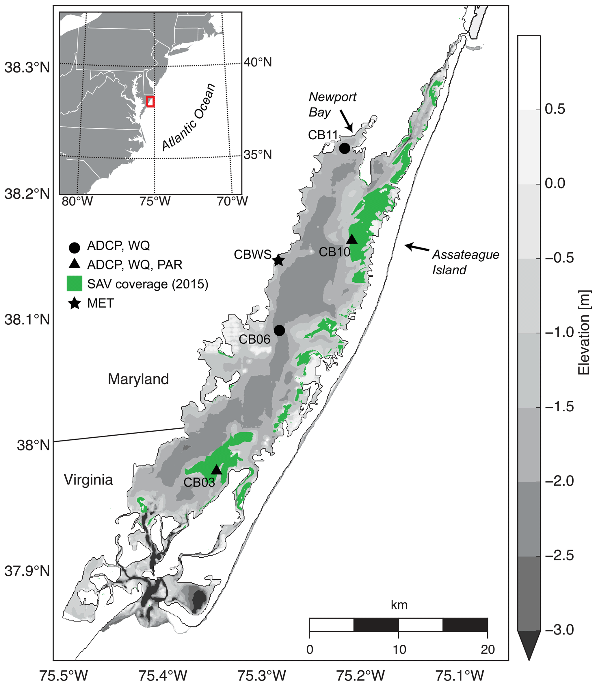
Figure 1Location map with bathymetry relative to mean sea level, instrument locations, and submerged aquatic vegetation coverage from the Virginia Institute of Marine Science annual SAV mapping survey (http://web.vims.edu/bio/sav/, last access: 1 October 2019). ADCP refers to acoustic current Doppler profiler; WQ refers to water-quality sonde; PAR refers to paired upper–lower PAR sensors; MET refers to meteorological parameters at site CBWS (Chincoteague Bay weather station).
The coastal ocean tide range approaches 1 m but is attenuated to less than 0.1 m in the center of the bay, where water levels are dominated by wind setup and remote offshore forcing (Pritchard, 1960); subtidal water-level fluctuations throughout the bay approach 1 m (Nowacki and Ganju, 2018). River and watershed constituent inputs are minimal, with the highest discharge and lowest salinities near Newport Bay in the northwest corner of the bay. Atmospheric forcing is characterized by episodic frontal passages in winter with strong northeast winds; summer and fall exhibit gentler southwest winds. Waves within the bay are predominantly locally generated, with substantial dependence on wind direction and fetch due to the alignment of the estuary along a southwest to northeast axis.
Wazniak et al. (2007) synthesized water-quality metrics for Chincoteague Bay, indicating high spatial variability in chlorophyll a, dissolved oxygen, and nutrient concentrations. Sites in the northern portion of the bay had generally poorer water quality, ostensibly due to higher nutrient loading and poorer flushing; Newport Bay had the lowest water-quality index. Fertig et al. (2013) identified terrestrial sources of nutrients to central Chincoteague Bay, though the precise source (anthropogenic vs. naturally occurring) could not be determined.
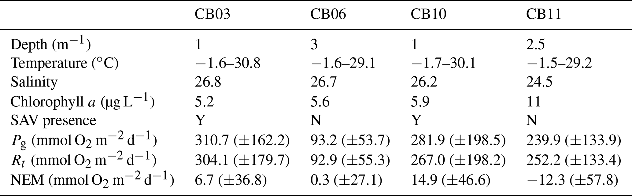
Table 1Water-column properties at the four study sites, SAV presence or absence, and metabolic rate estimates. Temperature data are minimum and maximum values (min, max), salinity is the annual mean, chlorophyll a is the annual mean, and metabolic rate estimates are means (± standard deviation) for the August–September (peak SAV growth) period. Standard deviations of all parameters are sufficiently large such that differences between means are not statistically significant except for Pg at site CB06 relative to site CB03.
2.2 Time series of turbidity, chlorophyll a, fDOM, dissolved oxygen, and light attenuation
Instrumentation was deployed from 10 August 2014 to 12 July 2015 (Suttles et al., 2017) at four locations in Chincoteague Bay (Fig. 1; Table 1). Instruments were recovered, downloaded, and serviced three times during that period (October 2014, January 2015, and April 2015). The sites were chosen to span a range of water depth, benthic type, and proximity to the coastal ocean; these represent a subset of the eight sites considered by Nowacki and Ganju (2018) in their sediment flux study. Here we include only the sites where light climate and/or water quality were measured comprehensively. Beginning in the southern portion of the estuary, site CB03 is within a seagrass meadow (primarily Zostera marina) on the eastern edge of the southern basin at 1 m of depth. Tide range is approximately 0.3 m (Nowacki and Ganju, 2018); the seabed is mainly composed of sand and silt, with organic content < 4 % (Ellis et al., 2016). Moving northward, site CB06 is within the main channel north of the nominal boundary between the northern and southern basins, with a silt-dominated bed, organic content of 6 %, no vegetation, a depth of 3 m, and a slightly diminished tide range of 0.2 m. Site CB10 is within a seagrass meadow on the eastern side of the northern basin, with a sand-dominated bed, < 4 % organic content, 1 m of depth, and a tide range of 0.15 m. Lastly, site CB11 is in the central basin of Newport Bay within the northwest portion of the estuary at a depth of 2.5 m with a tide range of 0.2 m. The seabed at this site is silt-dominated, with the highest observed organic content (> 8 %). A meteorological station was deployed at site CBWS, approximately 3.8 m above the water surface at Public Landing, Maryland, on the central western shore of Chincoteague Bay. Seagrass presence or absence was confirmed visually during instrument deployments; SAV bed area was obtained from the Virginia Institute of Marine Science Submersed Aquatic Vegetation Monitoring Program, which mapped SAV area from aerial imagery acquired annually in 2014 and 2015 (http://www.web.vims.edu/bio/sav/, last access: 1 October 2019; Orth et al., 2016).
The shallow-water platform described by Ganju et al. (2014) was deployed at sites CB03 and CB10 within sandy patches of the seagrass meadows. The platform was designed to measure hydrodynamic, biogeochemical, and light parameters in the bottom half of a 1 m water column and consists of an RBR Virtuoso D|Wave pressure recorder (±0.05 % accuracy); a pair of WET Labs ECO-PARSB self-wiping photosynthetically active radiation (PAR, 400–700 nm; ±5 % accuracy) sensors; a YSI EXO2 multiparameter sonde measuring temperature, salinity, turbidity, dissolved oxygen, chlorophyll a fluorescence, fluorescing dissolved organic matter (fDOM, a proxy for CDOM), pH, and depth (accuracies of ±0.2 ∘C, 0.2 psu, 0.3 FNU, 0.1 mg L−1, N/A, N/A, 0.2 pH units, 0.004 m; N/A indicates inapplicability of accuracy values for chlorophyll a and fDOM, which are dependent on the user-specific accuracy of the serial dilutions); and a Nortek Aquadopp acoustic Doppler current profiler measuring water velocity profiles (2 MHz standard at CB10 and 1 MHz high resolution at CB03; ±1 % accuracy). All instruments except for the upper PAR sensor were mounted at 0.15 m above the bed (m a.b.) on a weighted fiberglass grate approximately 1 m×0.5 m. The lower PAR sensor was recessed inside a PVC tube protruding from the bottom of the frame. The upper PAR sensor was mounted at 0.45 m a.b.; the upper and lower sensors provide an estimate of light attenuation KdPAR over the PAR spectrum (400–700 nm), calculated as
where dz is the distance between the two PAR sensors (0.3 m in this case). Light attenuation was calculated only between the hours of 10:30 and 15:30, when the angle of the sun relative to the deployment location was closest to 0∘. All sensors sampled at 15 min intervals, except for the wave recorders, which burst-sampled at 6 Hz every 3 min. Temperature, turbidity, and inner filter effects (IFEs) have been shown to alter fDOM measurements (Baker, 2005; Downing et al., 2012). We corrected fDOM measurements to account for temperature, turbidity, and IFE according to Downing et al. (2012). Measurements of fDOM at turbidities > 50 NTU were removed due to interference with the fluorescence signal. Chlorophyll a concentration was calculated from sensor-based fluorescence measurements by regressing fluorescence against discrete measurements of chlorophyll a made on four dates (August and October 2014, January and April 2015) at all stations (Fig. S1 in the Supplement). In short, water was collected in the field at the time of sensor sampling and filtered through 0.7 µm GF/F filters, which were wrapped in foil and frozen until laboratory analysis using standard methods (EPA Method 445.0). Non-photochemical quenching was accounted for by removing fluorescence measurements during periods of daylight (upper PAR sensor > 150 W m−2, or ∼40 % of the record) and interpolating to fill gaps. Platforms at sites CB06 and CB11 were identical to platforms at CB03 and CB10 except for the omission of PAR sensors. Light attenuation at those sites was estimated using the model of Gallegos et al. (2011), discussed below; this enabled comparison between vegetated and unvegetated sites using the same fundamental variables to compute light attenuation.
Quality control and quality assurance checks were performed on all data and are described in detail in the data report (Suttles et al., 2017). These included removal of obvious spikes in individual parameter time series using either a recursive filter or median filter technique, in which values that changed from one time point to the next by more than a set threshold were flagged and replaced with a fill value (e.g., −9999). Pre-deployment calibrations and a post-deployment check were performed on all EXO2 sensors following YSI procedures outlined in the EXO User Manual (Revision F). Linear corrections were obtained from either post-deployment calibration checks or differences between in situ values from a fouled sensor and from a cleaned, calibrated sensor at the beginning of the next deployment. If data were obviously fouled and corrections were not possible, the data were replaced with fill values. WET Labs ECO-PARSB instruments were checked to verify that counts were above their “dark” count (low-count) thresholds; therefore, legitimate data collected during night were also discarded. All subsurface pressure data were corrected for changes in atmospheric pressure by using local barometric pressure data, from the meteorological station at CBWS when available, to give a more accurate representation of pressure caused by the overlying water.
We investigated the frequency response of constituents using spectral density estimates (Welch's overlapped segment averaging estimator) and their uncertainties (Bendat and Piersol, 1986) for dissolved oxygen, turbidity, chlorophyll a, and fDOM. Uncertainty bounds on the spectra were used to test if differences in spectral density between sites were significant, with nonoverlapping uncertainty envelops suggesting significant differences. We also performed wavelet coherence analyses (Grinsted et al., 2004) between site CB03 (shoal) and CB06 (channel) for each constituent; wavelet coherence indicates the covariability of two signals at varying frequencies through time and can identify mechanistic linkages between processes that have complex temporal coupling. The analysis was limited to these two sites due to the more complete data coverage. Statistics of the constituent time series (mean, maxima, and minima) were computed with the original 15 min data and with variable sampling intervals (1, 2, 24 h) to investigate the influence of sampling resolution on spatial variability in biogeochemical variables.
Further details on collection protocols and access to the time series data are reported by Suttles et al. (2017). The hydrodynamic results of this field campaign have been described in detail by prior studies (Ganju et al., 2016; Beudin et al., 2017; Nowacki and Ganju, 2018); for the purposes of this paper we focus on the spatiotemporal variability of constituent concentrations and light attenuation.
2.3 Estimation of light attenuation contributions
We estimated light attenuation (for periods with missing PAR data or at sites with no PAR data) and relative contributions from turbidity, chlorophyll a, and CDOM using the method of Gallegos et al. (2011). This formulation computes spectral attenuation in terms of suspended and dissolved constituents including the effects of water, CDOM, phytoplankton, and non-algal particulates (NAPs; e.g., detritus, minerals, bacteria). We include absorption by four components: (1) absorption by water was assumed to follow the spectral characteristics of pure water; (2) CDOM absorption was taken as proportional to the fDOM concentration, with a negative spectral slope (Bricaud et al., 1981) set to sg=0.02 nm−1 (Oestreich et al., 2016); (3) phytoplankton absorption was proportional to chlorophyll a concentration and with the spectrum shape normalized by the absorption peak at 675 nm (initial value for peak absorption was taken as m2 (mg chl a)−1, within the range provided by Bricaud et al., 1995); and (4) non-algal absorption was taken as proportional to the suspended sediment concentration with a spectral shape (Bowers and Binding, 2006) that included a baseline of cx1=0.0024 m2 g−1 (Biber et al., 2008), an absorption cross section of cx2=0.04 m2 g−1 (Bowers and Binding, 2006), and a spectral slope of sx=0.009 nm−1 (Boss et al., 2001). The backscattering ratio of water was set at 0.5, while CDOM is considered non-scattering (Mobley and Stramski, 1997), and the particulate effective backscattering ratio bbx was initially set at 0.017.
Given the high variability in turbidity and suspended sediment concentrations due to wind-wave resuspension, we varied the value of bbx as a function of turbidity to achieve the best agreement between the model and observations. At turbidity below 50 NTU, bbx is constant at 0.017 and then linearly declines to 0.0024 at turbidities above 220 NTU. This modification implies that backscattering by mineral particles dominates at low turbidities, while large organic aggregates dominate at the highest turbidities (Gallegos et al., 2011), and has the effect of enhancing attenuation by particulate-induced absorption at the highest turbidities. The lowest values of the backscattering-to-scattering ratio bbx in the literature range from 0.005 (Snyder et al., 2008) to about 0.002 (Chang et al., 2004). The chosen value of 0.0024 was obtained from Loisel et al. (2007). Morel and Bricaud (1981) described the bbx ratio as decreasing with increasing absorption, which would be consistent with high-turbidity situations. McKee et al. (2009) described a decrease in the bbx ratio with increasing concentrations in a mineral-rich environment. The maximum sediment concentrations (15 mg L−1) in that study were higher than previously mentioned studies but smaller than concentrations observed in this environment (Nowacki and Ganju, 2018). Determining the appropriate backscattering ratio at high turbidities is still poorly constrained, and the minimum value used in this study might even be an overestimation (a sensitivity analysis is described in Sect. 3.1). The calibration of the light model at shoal sites (CB03 and CB10) and subsequent application at channel sites assume that the vertical variability in the bottom 0.3 m of the water column is similar among these sites.
2.4 Net ecosystem metabolism
The basic concept and method for computing community production and respiration (and ecosystem metabolism) were developed by Odum and Hoskin (1958) and, with numerous modifications, have been used since for estimating these rate processes in streams, rivers, lakes, estuaries, and the open ocean (Caffrey, 2004; Howarth et al., 2014). The technique is based on quantifying increases in oxygen concentrations during daylight hours and declines during nighttime hours as ecosystem rates of net primary production and respiration, respectively. The sum of these two processes over 24 h, after correcting for air–sea exchange, provides an estimate of net ecosystem metabolism. We utilized continuous oxygen concentration measurements at four locations in Chincoteague Bay (CB03, CB10, CB06, CB11) to compare differences in net ecosystem metabolism across sites and across habitats (phytoplankton- versus SAV-dominated, channel versus shoal). We computed daily estimates of gross primary production (Pg), ecosystem respiration (Rt), and net ecosystem metabolism (NEM ) using the approach of Beck et al. (2015), which utilizes weighted regression to remove tidal effects on dissolved oxygen time series. The changes in dissolved oxygen concentrations used to compute metabolic rates were corrected for air–water gas exchange using the equation
where D is the rate of air–water oxygen exchange (mg O2 L−1 h−1), Ka is the volumetric aeration coefficient (h−1), and Cs and C are the oxygen saturation concentration and observed oxygen concentration (mg O2 L−1), respectively. Ka was computed as a function of wind speed measured at a weather station installed at a dock (near CB10; Suttles et al., 2017). Details of the air–water gas calculation are incorporated into the R package WtRegDO (Beck et al., 2015) and described in detail in Thebault et al. (2008). The calculations utilized salinity, temperature, and dissolved oxygen time series from the sensors at each platform, as well as atmospheric pressure and air temperature data from a nearby buoy (OCIM2 – 8570283 at the Ocean City Inlet, Maryland).
The oxygen data used to make metabolic computations were obtained from sensors deployed near the bottom in relatively shallow waters. Our metabolic computations assume that the water column is well mixed, which is necessary for the air–water flux correction to be valid and for the oxygen time series to be representative of the combined water column and sediments (e.g., Murrell et al., 2018). We tested the validity of this assumption at our two deeper sites (which were 2–3 m deep) using monthly vertical profile data for dissolved oxygen, temperature, and salinity from the Maryland Department of Natural Resources from 1999 to 2014. These data indicate instantaneous vertical dissolved oxygen differences of > 1 mg L−1 on occasion over the 15-year record, generally during the productive summer months. The long-term mean vertical oxygen difference, however, was less than 0.5 mg L−1 during September to May but between 0.5 and 0.9 mg L−1 during June–August, indicating that although we did not measure vertical gradients during our study, they do occasionally develop.

Figure 2Time series of wave height, upper and lower PAR, KdPAR, turbidity, chlorophyll a, and fDOM at vegetated shoal site CB03.
3.1 Time series of turbidity, chlorophyll a, fDOM, dissolved oxygen, and light attenuation
Turbidity ranged from near zero to a maximum of over 400 NTU at site CB06 during a winter storm (December 2014) that induced waves exceeding 0.7 m (Figs. 2–5). The highest peak turbidities were observed at CB06, while sites CB03, CB10, and CB11 had similar statistical distributions of turbidity (Table 3), though the differences between mean values over the entire period were not statistically significant (Table 3). Turbidity at shoal sites was highest in the winter, between November and April, while turbidity at site CB06 did not display a similar seasonal signal. In general, tidal resuspension appeared to be minimal, although tidal advection after large wind-wave resuspension events was observed (Figs. 2–5). Spectrally, most of the energy in the turbidity signal was found at subtidal frequencies (i.e., > 1 d), with little correspondence between sites at tidal frequencies (Fig. 6).
Chlorophyll a concentrations peaked just below 50 µg L−1 at site CB11 and below 30 µg L −1 at all other sites (Figs. 2–5). Mean chlorophyll a concentrations were not statistically different across sites but were nonetheless twice as high at CB11 (Table 1). The largest concentrations were observed in winter during resuspension events, likely representing the resuspension of benthic microalgae, and during a broad spring bloom during March–April 2015. All sites showed a large decrease in chlorophyll a concentration during a period of ice formation in late February 2015, when advection and resuspension were largely halted in the estuary. Despite removing effects of non-photochemical quenching, an attenuated diel signal remains in the spectra that may be a partial artifact or consistent with day–night variations in PAR (Fig. 6). The diurnal signal was comparable across all stations and was stronger than the tidal signal (Fig. 6).
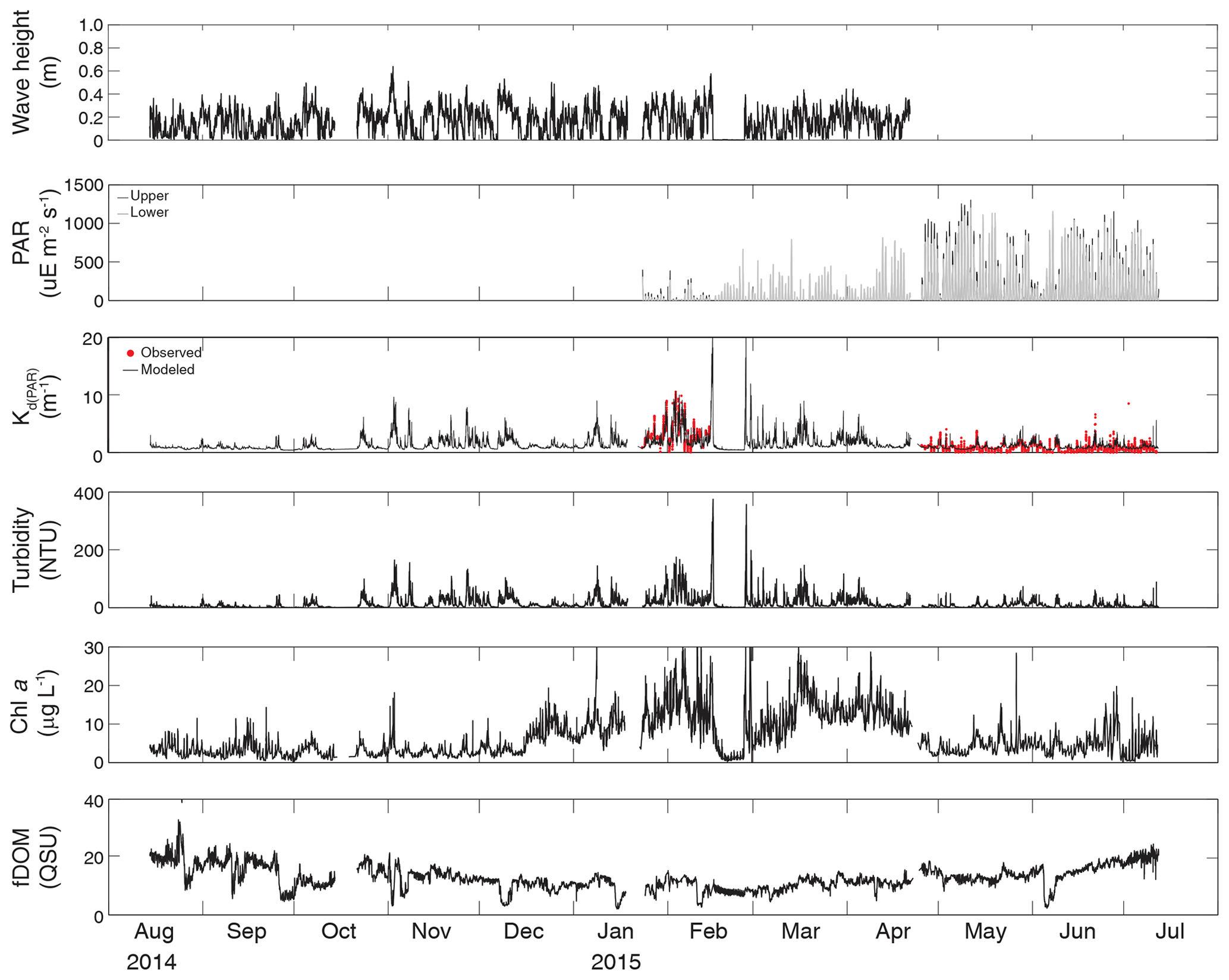
Figure 3Time series of wave height, upper and lower PAR, KdPAR, turbidity, chlorophyll a, and fDOM at vegetated shoal site CB10.

Figure 4Time series of wave height, modeled KdPAR, turbidity, chlorophyll a, and fDOM at unvegetated channel site CB06.
Concentrations of fluorescing dissolved organic matter (fDOM) varied between 0 and 70 QSU, with the highest peak values over the overlapping period of record observed at CB11 in Newport Bay (Figs. 2–5). Concentrations were similar between the other sites, with the lowest fDOM in the winter, possibly due to reduced dissolved organic material production in the surrounding watershed and ultimately in freshwater runoff to the estuary. Periodic large decreases in fDOM coincided with increases in turbidity due to wind-wave resuspension; despite correcting the fDOM time series for turbidity interference, the fluorescence measurement was likely attenuated beyond correction. Most of the energy in the fDOM signal was at subtidal frequencies (Fig. 6); there was a distinct peak at the M2 tidal frequency (12.42 h or ∼0.5 d) corresponding to the advection of fresher, fDOM-elevated water on ebb tides.
Dissolved oxygen percent saturation ranged from a minimum of 19 % at site CB11 in the summer to a maximum of over 200 % at site CB10 (Fig. 7), with maximum diel variability in the summer. The channel sites (CB06 and CB11) showed substantially attenuated diel variations compared to the shoal sites (CB03 and CB10). Diel fluctuations in the winter were typically less than the subtidal changes. Spectral analysis clearly shows the dominance of 24 h diel fluctuations at all sites (Fig. 6), with higher energy at the vegetated shoal sites (CB03, CB10).
Table 2Median light attenuation and relative contributions from turbidity, chlorophyll a, and fDOM. The remainder of the light attenuation contribution is from water (not shown) and is equivalent between sites.
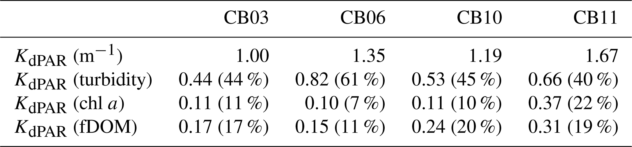

Figure 5Time series of wave height, modeled KdPAR, turbidity, chlorophyll a, and fDOM at unvegetated channel site CB11.
Direct measurements of KdPAR at sites CB03 and CB10 were partially confounded by instrument fouling and the malfunction of one or both sensors on each platform. Nonetheless, we successfully captured a wide range of conditions, with peak light attenuation of approximately 10 m−1 occurring at sites CB03 and CB10 in the winter during a sediment resuspension event (Figs. 2–5). Median KdPAR was approximately 1 m−1 at both shoal sites, but event-driven magnitudes exceeded 2 m−1 multiple times during the deployment. The KdPAR data were used to calibrate the light model (Fig. S2), which we implemented to reconstruct missing data at sites CB03 and CB10, as well as to estimate light attenuation at sites CB06 and CB11 where constituent concentrations were measured but no light data were collected. The full time series of estimated light attenuation at the four sites demonstrates the strong seasonal variability of light attenuation at all sites (Figs. 2–5), with peak attenuation occurring during winter storms. Wave-induced sediment resuspension and advection were responsible for increased turbidity, which accounted for approximately 40 % of the light attenuation at sites CB03, CB10, and CB11 and 61 % at site CB06. Light attenuation at site CB11, with its proximity to freshwater and nutrient sources, was highest overall during the overlapping period of record and more highly influenced by chlorophyll a and fDOM than at other sites. Median KdPAR was highest at the two unvegetated channel sites and lowest at the two vegetated shoal sites (Table 2), though the period means are not statistically different. Turbidity, the strongest driver of KdPAR, was generally lower during the warm season at the vegetated shoal sites, and the turbidity generated for a given wind-wave-induced bed shear stress was significantly reduced in summer at the vegetated sites, while there was no significant seasonal variation in the turbidity–shear stress relationship at unvegetated channel sites (Fig. 8).
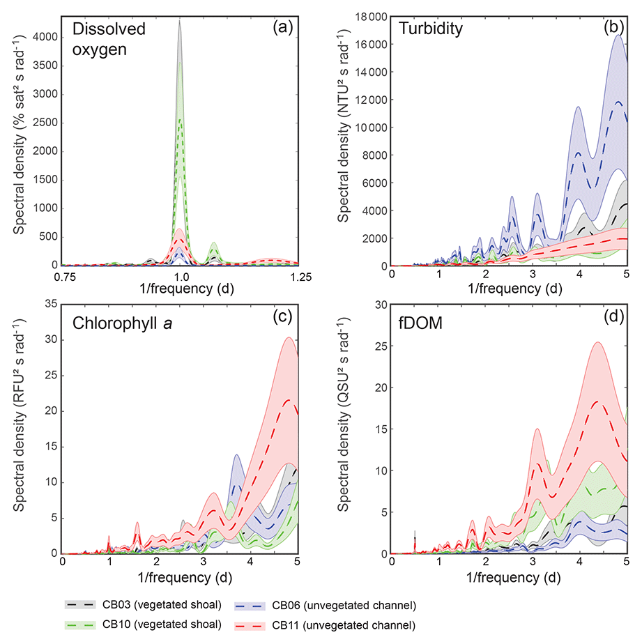
Figure 6Spectral density estimates for (a) dissolved oxygen, (b) turbidity, (c) chlorophyll a, and (d) fDOM at all four sites. Shaded areas indicate 90 % uncertainty bounds of spectral density estimates. The dissolved oxygen spectra for site CB03 are beneath the spectra for site CB10. A defined peak of fDOM can be seen at 12.42 h or 0.5 d (d), though the lower-frequency spectral density is higher overall.
Sediments at site CB06 and CB11 tend to be finer (Ellis et al., 2016) and may be more susceptible to flocculation, which would induce error in the light model. Therefore, we ran the light model with variation in the maximum particle backscatter ratio (bbx), which is particle-size-dependent. An increase in flocculated suspended sediment would increase this ratio, thereby increasing the light attenuation and causing a larger difference in light attenuation between the sandy, vegetated sites and the siltier, unvegetated sites. Modifying the peak value as described above from 0.017 to 0.025 (47 % increase; 0.025 value was used for a different mud-dominated estuary by Ganju et al., 2014) increased the median light attenuation at CB06 by 17 % (from 1.35 to 1.58 m−1) and at CB11 by 11 % (from 1.67 to 1.86). Therefore, the spatial variability in light attenuation is likely robust and not confounded by variability in particle size.
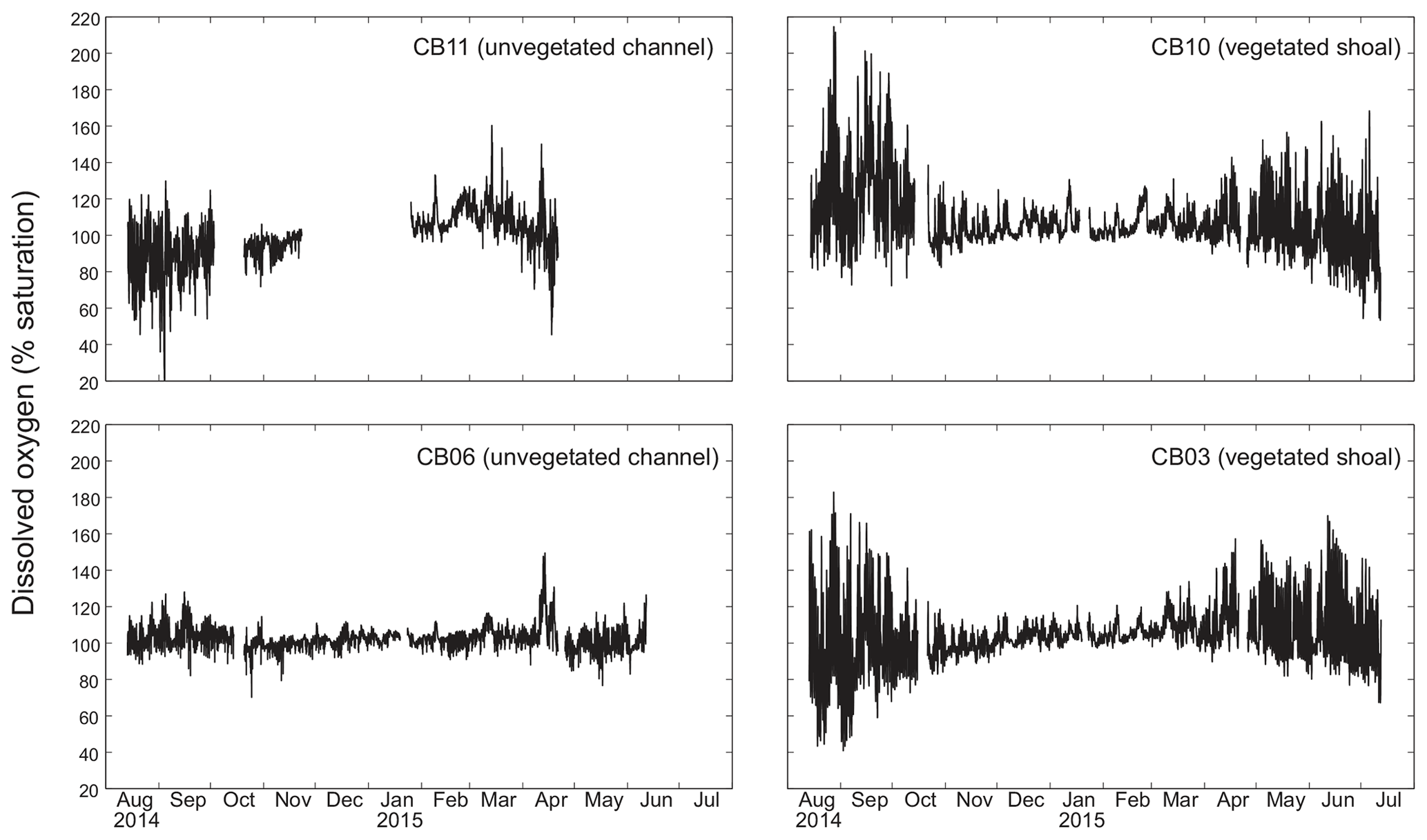
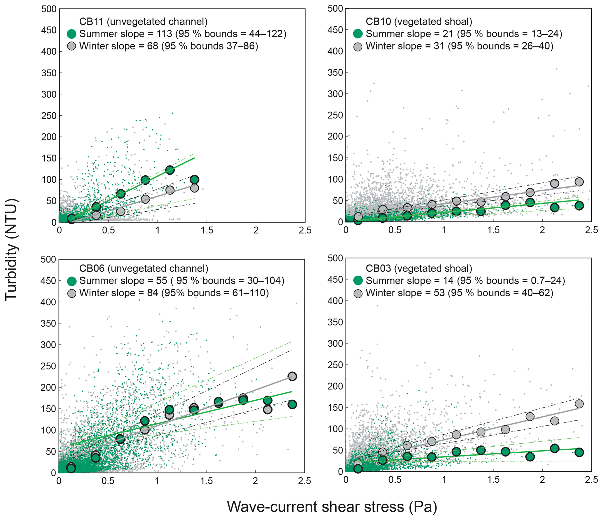
Figure 8Relationship between combined wave-current-induced bed shear stress and turbidity at four sites, with repeated-median linear regressions of bin-averaged values over summer (May–September) and winter (October–April). Larger slopes indicate a stronger relationship between shear stress and turbidity. Dashed lines indicate 95 % confidence bounds on slopes; bounds overlap at channel sites, indicating a lack of significant difference between seasons, while bounds do not overlap at shoal sites, indicating a significant seasonal difference in the stress–turbidity relationship, likely caused by vegetation.
The wavelet coherence of dissolved oxygen between site CB03 and site CB06 was maximized at diel timescales (Fig. 9), corresponding to covarying oscillations due to daytime production and nighttime respiration. Coherence was also high at lower frequencies, especially during winter when oscillations at both sites were small due to reduced production and respiration. Turbidity was coherent between channel and shoal sites primarily at subtidal timescales, corresponding to episodic multiday resuspension events and generally high turbidity during most of the winter. Phase lag was minimal during times of high coherence for both of these parameters. Coherence for both chlorophyll a and fDOM was minimal throughout the year, though the former demonstrated sporadic coherence at diel and multiday timescales. The December–April period of generally high chlorophyll a was similar between these sites and manifested as increased coherence at ∼512–1024 h (21–42 d).
Table 3Mean, minima, and maxima for four water-quality parameters at four sites with variable temporal sampling resolution over the entire period of record. The standard deviations (SD) of all parameters at original temporal resolution are sufficiently large such that differences between means are not statistically significant, except for fDOM at sites CB10 and CB11 relative to site CB06.

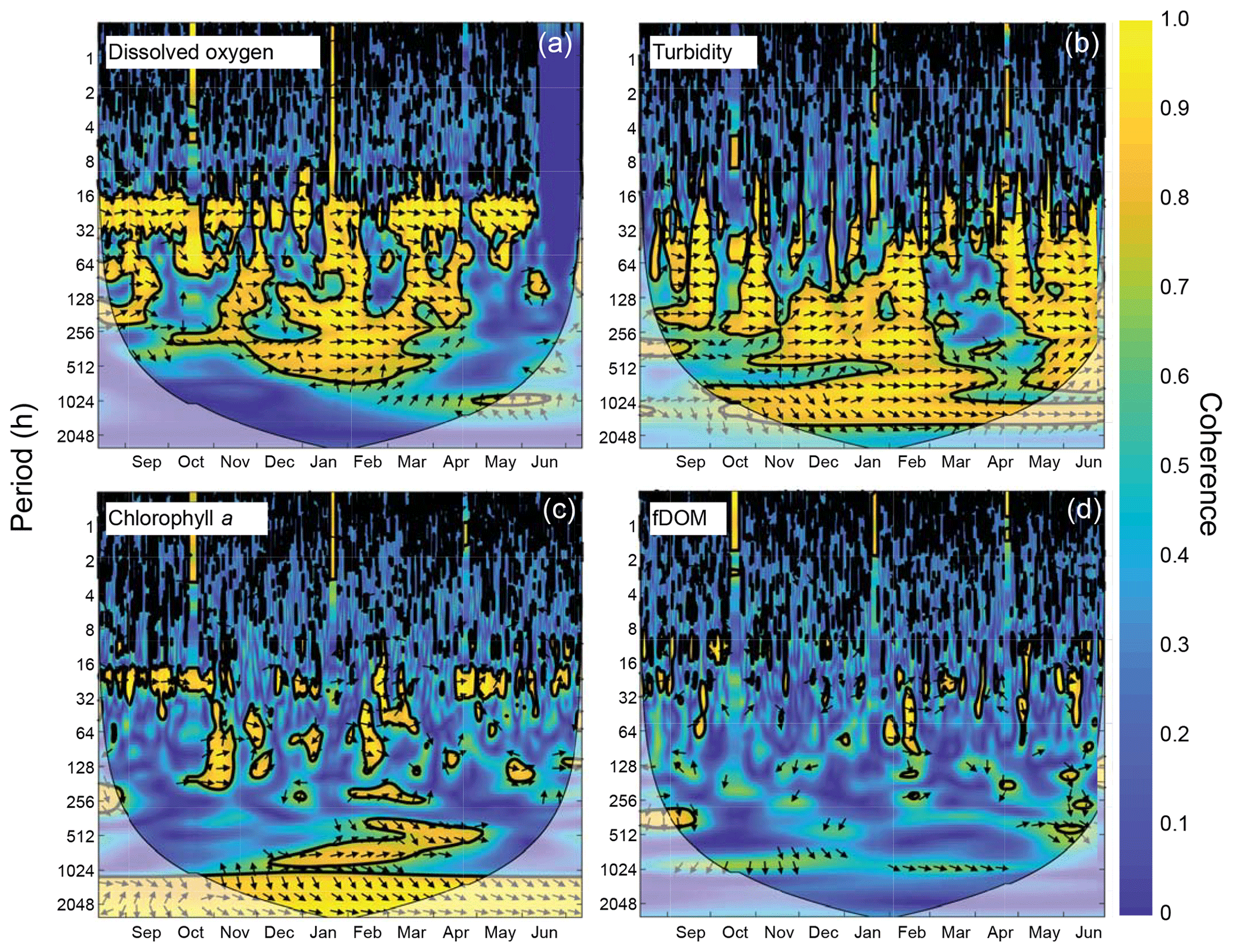
Figure 9Wavelet coherence between time series at sites CB03 (vegetated shoal) and CB06 (unvegetated channel) for four water-quality parameters: (a) dissolved oxygen, (b) turbidity, (c) chlorophyll a, and (d) fDOM. Increased coherence at a given period indicates covariability of the time series at that time; for example, increased coherence at ∼24 h for dissolved oxygen during most of the record indicates covarying diel oscillations at both sites during most of the year. The direction of arrows indicates phase; arrows pointing to the right indicate that signals are in phase. Shaded areas near the bottom of each panel indicate areas that are not statistically robust and should be interpreted with caution.
Statistics of the constituent time series were computed with temporal sampling intervals of 15 min (original sampling interval) and 1, 2, and 24 h (Fig. 10; Table 3). While mean values were minimally altered, minima and maxima were significantly dampened for dissolved oxygen and turbidity. At site CB11, the original sampling interval captured a hypoxic event in September 2014 with a minimum value of 19 % dissolved oxygen, while daily sampling yielded a minimum of 55 %, above the hypoxic threshold. Similarly, at site CB10 supersaturation led to a maximum of over 200 % dissolved oxygen, while daily sampling yielded a maximum of 152 %. Maximum values of turbidity were similarly attenuated by daily sampling (Table 3). The effect of these sampling intervals is discussed later in the paper.
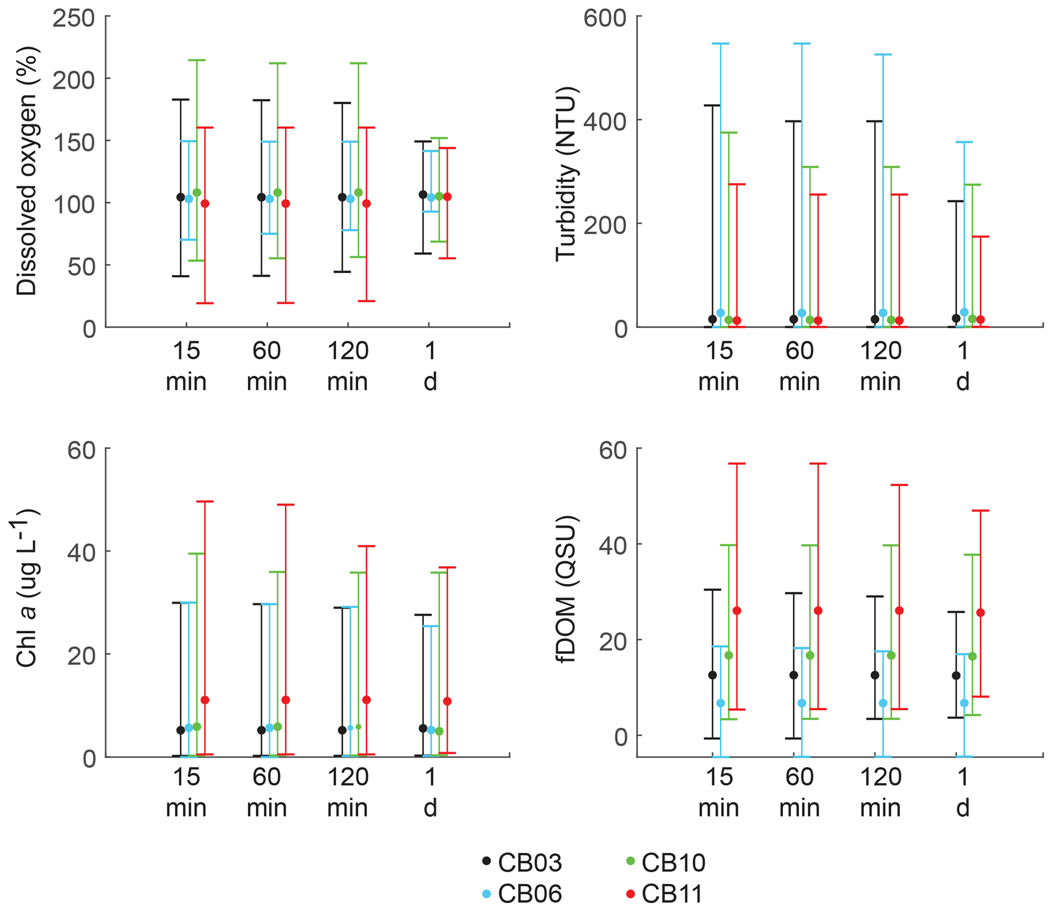
Figure 10Mean (dots), maxima, and minima (bars) for each parameter using different temporal sampling intervals (15 min; 1, 2, 24 h). Spatial variability in dissolved oxygen is most impacted by coarse temporal resolution, with spatial differences in minima and maxima largely eliminated at a resolution of 1 d.
3.2 Net ecosystem metabolism
Estimates of ecosystem metabolism displayed strong seasonal variability, with elevated rates of Pg and Rt during warm months across all stations (Figs. 11, 12; Table S1 in the Supplement). High rates of Pg and Rt persisted between May and September, when temperature and PAR peaked seasonally, and were consistently lower during November to March (Figs. 11, 12); Rt was exponentially related to temperature across sites (although less so at CB06). Daily metabolic rates were clearly higher at vegetated shoal sites (CB03, CB10), consistent with the strong diurnal signal in oxygen at these sites (Figs. 6, 7) and the presence of seagrass (Table 1). Temperature was strongly associated with rates of respiration across all sites, and respiration reached peak values under conditions of high temperatures and high rates of Pg (Fig. 12). Gross primary production and respiration were largely balanced across all sites, but the frequency of daily net autotrophy (Pg > Rt) was higher at the vegetated sites.
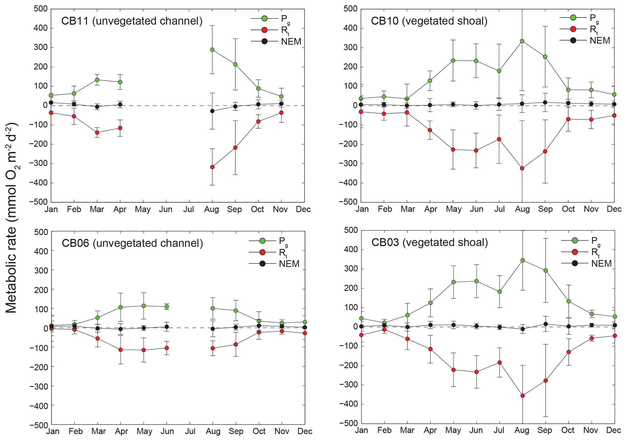
Figure 11Monthly estimates of gross primary production (Pg), respiration (Rt), and net ecosystem metabolism (NEM) at four sites. Measurements span August 2014 through July 2015, and therefore the time axis begins in August 2014 and wraps back to January 2015.
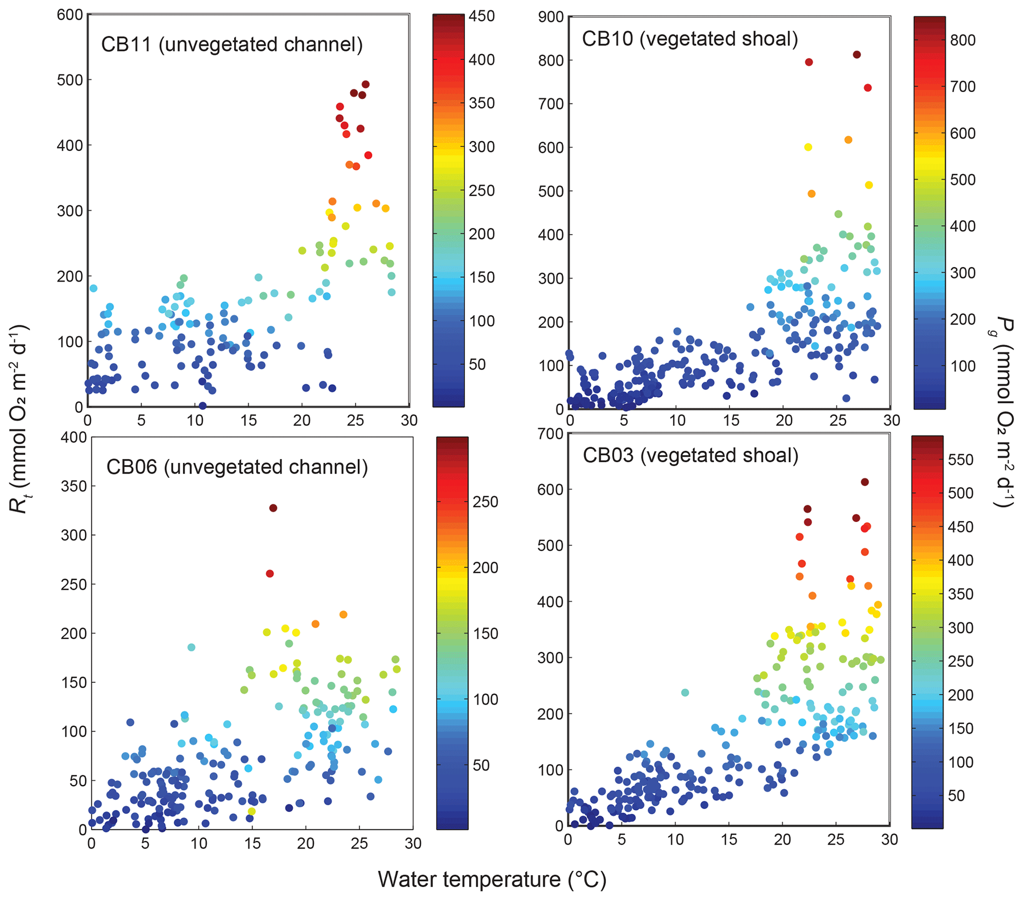
Figure 12Relationship between respiration (Rt) and water temperature at four sites, with data coloration scaled to gross primary production (Pg).
The relationship between rates of Pg and light availability was site-specific. At the vegetated sites, CB03 and CB10, Pg and KdPAR were significantly negatively correlated, with high rates of Pg occurring during the periods of lowest KdPAR and highest surface PAR (Fig. 14). At CB06 and CB11, variations in Pg and KdPAR were not significantly correlated, and KdPAR was higher and Pg was lower at these sites than at CB03 and CB10 (Tables 1, 2; Figs. 13, 14). Over the entire record, mean values were not statistically different except for mean Pg between sites CB03 and CB06 (Table 1). In summary, the highest daily metabolic rates we measured occurred during warm periods in vegetated shoals, where wave attenuation by seagrass reduced turbidity and KdPAR.
Net ecosystem metabolism and other water-quality parameters are typically measured over limited spatial (e.g., single point) and temporal (e.g., days to weeks) scales. An analysis of a comprehensive suite of high-frequency biological and physical measurements in Chincoteague Bay over an annual cycle revealed the primary drivers of light attenuation, the role of light attenuation in driving variations in gross primary production, the primary timescales of biogeochemical variability, and the effect of habitat type (i.e., vegetated versus unvegetated; nutrient enrichment) on oxygen variability and net ecosystem metabolism. Turbidity dominated light attenuation variability and varied considerably at 1–7 d timescales, consistent with the frequency of storm passage. Storm-associated wind waves were the specific driver of resuspension and turbidity, and the reduction of bed shear stress and turbidity in SAV-dominated shoal environments during summer increased light availability in these habitats. As a consequence, Pg was substantially higher in SAV-dominated shoals compared with adjacent plankton-dominated sites, and Pg was negatively correlated with KdPAR in the shoals, highlighting the role of short-term variability in light availability driving Pg. High rates of Pg and Rt in shoal environments led to much higher diurnal and seasonal-scale variability in dissolved oxygen in these habitats. Though we do not have direct estimates of microalgal production partitioned between sediments and the water column at any of our sites, the sediment surface is nearly covered by SAV and macroalgae at the vegetated sites; therefore, we expect that benthic microalgal production is low. At site CB11, KdPAR values indicate that very little light reaches the bottom, so we presume that water-column microalgae are dominant. For site CB06, we cannot constrain the partitioning between the two environments.
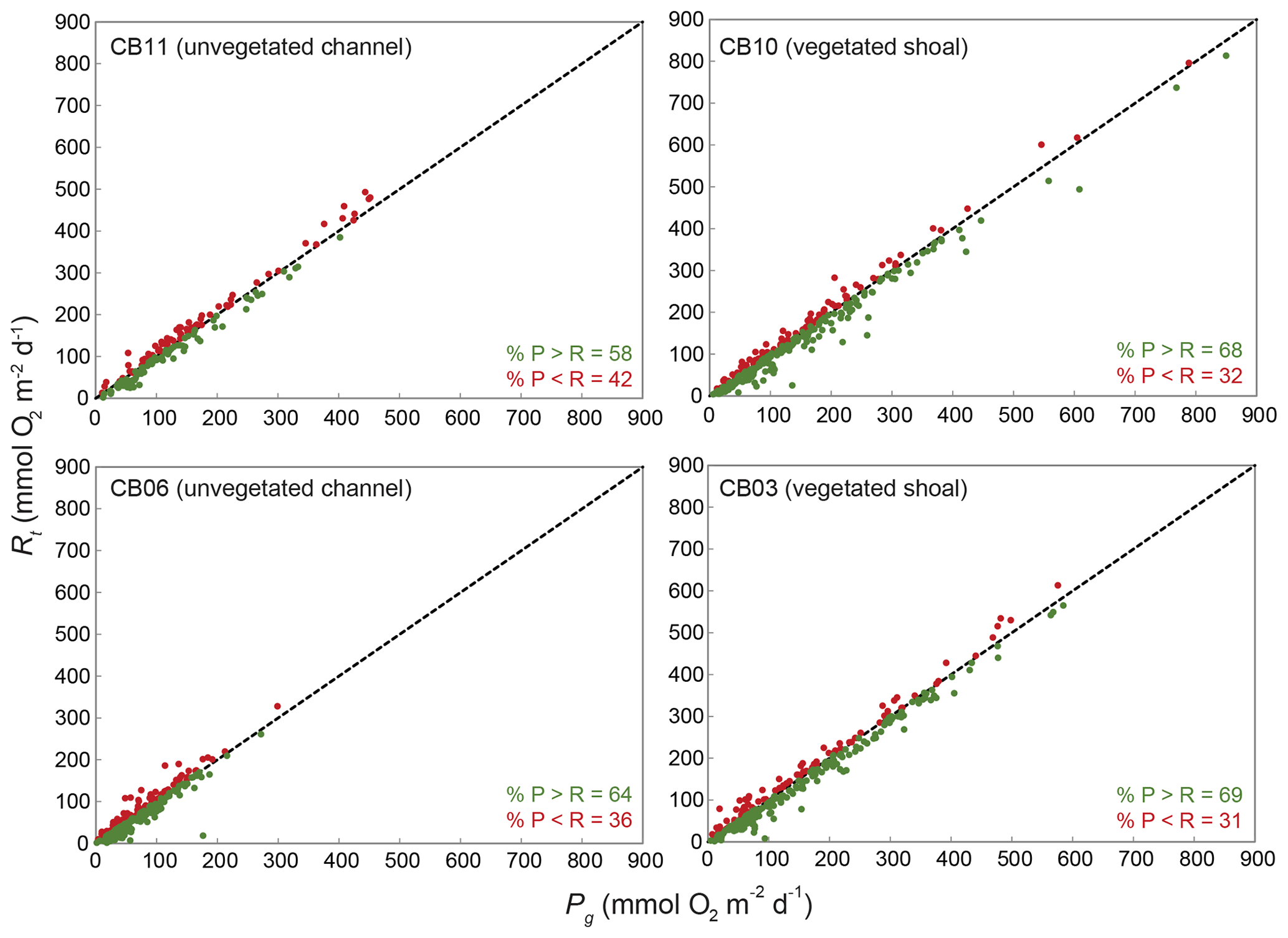
Figure 13Relationship between gross primary production (Pg) and respiration (Rt) at four sites; line of 1:1 agreement shown.
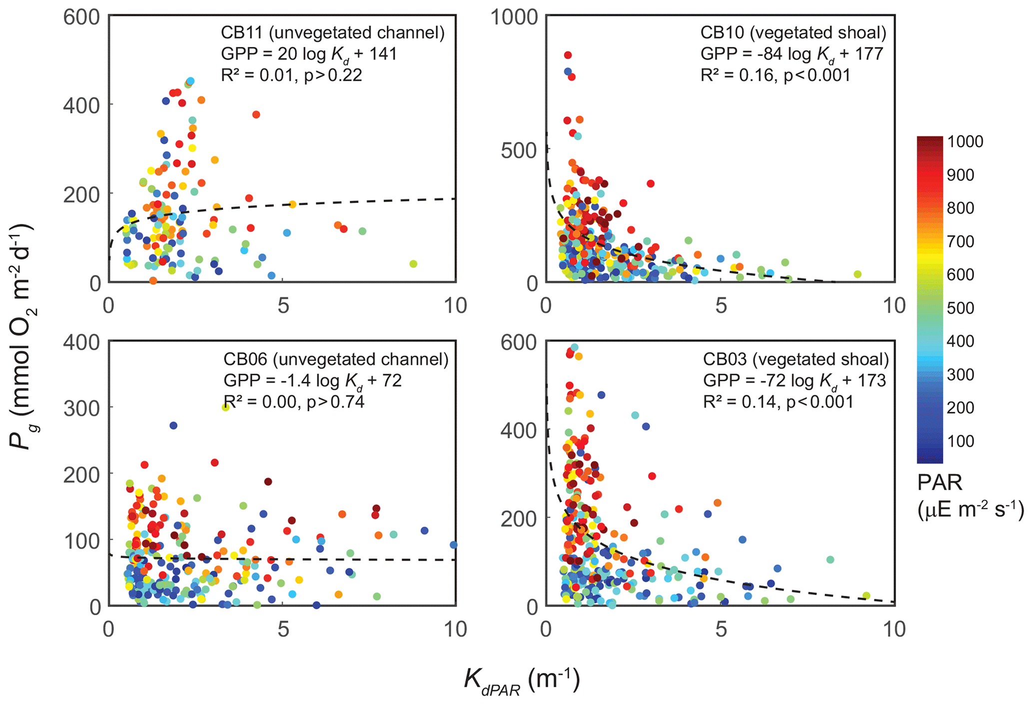
Figure 14Relationship between light attenuation KdPAR and gross primary production (Pg), with coloration indicating surface photosynthetically active radiation (PAR; µE m−2 s−1) measured at the weather station. The linear model was fitted to Pg as a function of log (KdPAR). The relationship between Pg and KdPAR is significant at vegetated shoal sites but not significant at unvegetated channel sites.
4.1 Spatiotemporal variability of constituents
4.1.1 Interpretation of spectral signals
Spectral analysis of the constituent time series elucidates significant differences between channel and shoal sites, as well as longitudinally within the estuary. With regards to dissolved oxygen, the peak in diurnal energy at shoal sites is markedly stronger relative to channel sites, with no overlap in uncertainty bounds between channel and shoal sites, indicating higher local production and/or respiration due to SAV presence. Between sites CB03 and CB06, the diurnal peak in spectral density is reduced by 94 % and reduced by 83 % between site CB10 and CB11. The peak in spectral density was 30 % higher at CB03 than CB10, perhaps due to higher SAV biomass at that site. This indicates the dominant role of seagrass in controlling oxygen concentrations locally and the relatively weaker oxygen dynamics at the channelized, unvegetated sites. From a sampling perspective, this also suggests that interpreting oxygen dynamics with limited spatial resolution is confounded by heterogeneous benthic coverage.
The highest spectral densities for turbidity were observed at site CB06 across all frequencies. At the lowest frequencies corresponding to multiday storms, there was no overlap in the uncertainty bounds. Nowacki and Ganju (2018) showed that sediment fluxes at this site were an order of magnitude larger than the other three sites due to a strong response to wind events, which are typically multiday events. The central location of the site suggests that local sediment transport would respond consistently to the seasonally variable winds, which tend to act along the axis of the estuary. Resuspension over shoals on either end of the estuary and subsequent advection cause the spatial integration of resuspension processes throughout the estuary at this main channel site.
Spectral density peaks of chlorophyll a were similar between sites, with significant overlap across frequencies, but site CB11 demonstrated the highest total spectral density, primarily at subtidal frequencies. The reduced exchange with other portions of the estuary, local nutrient inputs, and longer residence times increase the potential for phytoplankton growth at this station, which is known to be locally eutrophic (Fertig et al., 2009). This coincides with the lowest oxygen minima across the four sites (Table 3), indicating eutrophication. Again, in regards to sampling strategies, characterizing spatial variability in eutrophication is confounded by the competing timescales of transport and biogeochemical processes.
While the tidal signal in fDOM was pronounced (peak at 12.42 h or 0.5 d), the bulk of the spectral density was in the lower-frequency band at sites CB10 and CB11 in the northern half of the estuary. This likely represents a longitudinal gradient in freshwater input, with decreased salinity in the north where inputs are largest. The inverse correlation between salinity and fDOM in Chincoteague Bay was identified in prior work (Oestreich et al., 2016) and highlights the roles of tidal circulation, residence time, and freshwater input in biogeochemical and light attenuation patterns.
4.1.2 Channel–shoal coherence of water-quality parameters
Wavelet coherence analyses demonstrate that though certain parameters are tightly coupled between channel and shoal, other parameters are not. The coherence of dissolved oxygen at diel and longer timescales, along with nearly no phase lag, is congruent with diel and seasonal patterns of production and respiration. The “breathing” of the estuary (Odum and Hoskin, 1958) appears to be a near-simultaneous process regardless of location and demonstrates the importance of local biogeochemical processes throughout the system. With regards to turbidity and sediment resuspension, the coherence at subtidal timescales indicates that channels integrate resuspension processes over the entire estuary; minimal phase lag suggests that a rapidly evolving local wave climate in response to episodic winds controls both resuspension and rapid advection through the channels (Nowacki and Ganju, 2018). Conversely, chlorophyll a demonstrates coherence only over the seasonal timescale, and therefore advection and other tidal processes do not appear to control the dynamic exchange of phytoplankton or benthic microalgae. Lastly, the lack of coherence in fDOM shows that freshwater input is relatively minor in the southern half of the estuary, and despite a significant peak in spectral density at the tidal timescale, the advection of freshwater (and fDOM) between channel and shoal is not significant. Despite a qualitatively coherent annual signal in fDOM, the analysis cannot detect coherence at this timescale with a single year of data. These complex relationships between parameters highlight both the intricate response to spatiotemporal variability in biophysical environments and the necessity of high-frequency, spatially comprehensive measurements to understand estuarine ecosystem behavior.
4.1.3 Influence of temporal sampling resolution on spatial variability
Many estuary sampling programs, including “citizen science” efforts, often collect one daily sample of water-quality parameters, including dissolved oxygen (Rheuban et al., 2016). Summers et al. (1997) demonstrated that month-long records of dissolved oxygen in a number of estuarine systems, resampled to replicate various noncontinuous sampling programs, were not able to identify oxygen minima. This study expands on that finding by mimicking sampling programs within one large estuary over an entire year. Though mean biogeochemical values were relatively insensitive to sampling interval, maximum values were significantly modulated for all parameters, while minimum values for dissolved oxygen were also affected. With regards to dissolved oxygen specifically, we find that daily sampling dampens the spatial variability in maxima and minima between sites. For example, a daily sampling program would not detect hypoxic conditions at site CB11 and would only observe a 13 % difference in dissolved oxygen compared to nearby site CB10, while the actual difference was over 30 %. This is relevant given the ubiquitous daily sampling programs in many estuaries, which cover numerous locations with infrequent sampling. This result suggests that characterizing differences in water-column conditions across space requires sampling at timescales finer than 1 d, especially in highly metabolic environments where diel oscillations in dissolved oxygen are large. Continuous monitoring at multiple locations in an estuary is difficult due to fouling and instrument limitations (e.g., power and memory), especially across large systems over an entire year. However, it may be more informative to conduct shorter-term, continuous monitoring deployments at select locations rather than daily monitoring at many locations. In the case of Chincoteague Bay, characterizing the oxygen environment would be possible with seasonal, month-long deployments at four sites. This type of data would yield both an accurate assessment of minimum and maximum values and allow spectral analysis to capture tidal-timescale variability.
4.2 Spatiotemporal variability of light attenuation
Light attenuation can appear to be controlled by uncoupled biological (i.e., nutrient loading and phytoplankton blooms) and physical (sediment resuspension) processes, but in reality the feedbacks between physics and biology are consistently present in estuaries. Wave-induced suspended sediment resuspension is primarily responsible for light attenuation in shallow lagoons like Chincoteague Bay, and seagrass clearly modulates the magnitude and spatiotemporal variability in sediment resuspension through the attenuation of wave energy (e.g., Hansen and Reidenbach, 2013). This wave-induced resuspension and turbidity occurs on the timescale of periodic wind events observed in this system. During summer months, when vegetation densities are ostensibly the highest, the dependence (i.e., slope) of turbidity on bed shear stress decreases significantly at the vegetated shoal sites, while it is not significantly different at the unvegetated channel sites (Fig. 8). In the winter, when seagrass is largely absent, the slope increases at the shoal sites, indicating the influence of seagrass on bed stabilization in the summer. The role of seagrass in modulating the physical environment is demonstrated by this improvement in light availability when vegetation reestablishes in the warmer months. Furthermore, the dependence of Pg on KdPAR at the vegetated shoal sites (Fig. 14) completes the positive feedback loop between benthic stabilization, sediment resuspension, light attenuation, and primary production. It is important to note that the seasonal change in resuspension response at the shallow sites may also be partially attributed to increased microphythobenthos coverage in summer. However, it is likely that in these vegetated sandy substrates, seagrass would dominate bed stabilization over benthic microalgae given shading and coarser sediment. In fact, the data of Ellis et al. (2016) indicate organic matter percentages of less than 2 % on the sandy shoals.
Our measurements underscore the ability of comprehensive continuous measurements to capture multiple scales of variation in light attenuation. For example, subsampling our light attenuation measurements under fair weather conditions (wave height < median) leads to the underestimation of median KdPAR by as much as 27 % (sites CB06 and CB10). Subsampling to periods with wave heights less than the 84th percentile leads to underestimation by 13 % (site CB06). The effect of these changes can be large if sparse data are used to assess trends in biogeochemical variables or to drive ecological models. In situations in which continuous monitoring of light attenuation is difficult, light modeling using continuous measurements of turbidity, chlorophyll a, and fDOM is a suitable proxy. With a reasonable number of discrete light attenuation samples, it is possible to calibrate a light model and estimate seasonal changes in contributions to light attenuation using the constituent measurements. This becomes useful when attempting to determine the relative influence of physical and biogeochemical processes on spatiotemporal variations in light attenuation and the potential benefits of restoration activities.
Apart from Newport Bay in the northwest corner of the estuary, Chincoteague Bay is relatively unimpacted by external nutrient and organic material inputs compared to other lagoonal systems on the US East Coast (e.g., Indian River Lagoon, Phlips et al., 2002; Great South Bay, Kinney and Valiela, 2011). For example, the relatively urbanized watershed surrounding Barnegat Bay, New Jersey, contributes larger nutrient loads to the northern portion of the estuary (Kennish et al., 2007); however, the highest light attenuation is observed in the southern portion, where sediment concentrations are highest due to the availability of fine bed sediment and wind-wave resuspension (Ganju et al., 2014). In fact, in Barnegat Bay light attenuation is lowest in the more eutrophic, poorly flushed (Defne and Ganju, 2015) northern portion due to coarser bed sediments and smaller wave heights (and less resuspension). In the more nutrient-enriched regions of the Maryland coastal bays north of Chincoteague Bay, chlorophyll a is also much higher and likely makes a larger contribution to light attenuation (Boynton et al., 1996). In contrast, spatial variability in the light field within Chincoteague Bay is driven by geomorphology (depth), the presence of submerged aquatic vegetation (CB03 and CB10), and the higher contribution of chlorophyll a at a nutrient-enriched site (CB11; Boynton et al., 1996). Thus, generalizing the light attenuation in back-barrier estuaries is hampered by these subtle, habitat-specific controls on attenuation, but improvements in continuous monitoring will lead to an increased understanding of these controls.
4.3 Spatiotemporal variability in metabolism and relationship with benthic ecosystem and light attenuation
Clear differences in the magnitude and timescales of oxygen dynamics were present across habitats in Chincoteague Bay. Spectral density at the diurnal timescale for dissolved oxygen was significantly higher at the two vegetated sites, where high rates of primary production during the day and associated respiration at night led to large changes in dissolved oxygen. Although this pattern is unsurprising given the high metabolic rates in these dense seagrass beds, this study is one of few studies that have clearly documented this pattern inside and outside SAV beds within an estuary over annual timescales. Elevated metabolic rates in macrophyte-dominated habitats relative to phytoplankton-dominated habitats have been documented in other systems (D'Avanzo et al., 1996), where the canonical C:N molar ratio of phytoplankton () is much less than that measured for Chincoteague Bay Z. marina (), indicating higher carbon and oxygen metabolism for a given amount of nitrogen (e.g., Atkinson and Smith 1983). Elevated magnitudes of daily oxygen change have also been associated with elevated phytoplankton biomass in Chincoteague Bay (e.g., Boynton et al., 1996) and other systems (e.g., D'Avanzo et al., 1996). This is consistent with the fact that the site at Newport Bay (CB11), which had the highest plankton chlorophyll a concentrations across all sites, had a larger spectral density for dissolved oxygen at the diel frequency than at CB06. Newport Bay is known to have elevated nutrient inputs and concentrations associated with land use in its watershed (Boynton et al., 1996), and spectral density for chlorophyll a was highest at this location (Fig. 6), suggesting that this site is responding to eutrophication.
Seasonal variations in metabolic rate estimates were typical of temperate regions but were variable across space. At all stations, rates of Pg and Rt were highest in warmer months when incident PAR and temperature are highest in this region, but rates were especially high in the later summer (August and September) at the vegetated sites. This late summer period is typically when SAV biomass is highest and where the self-reinforcing effect of wave attenuation, reduced resuspension, and reduced KdPAR allow for high rates of primary production (Figs. 8, 14). Indeed, the relationship between KdPAR and Pg was strongest at these vegetated sites (Fig. 14), displaying sensitivity of benthic primary production to light attenuation, which was dominated by turbidity. Elevated temperatures during this period also stimulate respiration (e.g., Marsh et al., 1986), which has been documented at the ecosystem scale in other SAV-dominated coastal systems (Howarth et al., 2014; Boynton et al., 2014). Seasonal variations in metabolic rates were comparatively lower at the unvegetated, non-eutrophic site (CB06), where low phytoplankton biomass and the absence of macrophytes lead to limited primary production and respiration rates.
The metabolic balance (ratio) between primary production and respiration is a metric of interest in coastal aquatic ecosystems as it provides an indication of whether the system is a relative source or sink of carbon with respect to the atmosphere (Stæhr et al., 2012). Many river-dominated estuaries and estuaries flanked by extensive tidal marshes are net heterotrophic, whereby respiration exceeds primary production (e.g., Kemp and Testa, 2011). Pg and Rt are often balanced or indicate modest autotrophy in shallow lagoons where SAV is present (e.g., Ferguson and Eyre, 2010; D'Avanzo et al., 1996). Autotrophy tends to persist in these habitats as submerged macrophytes like SAV generate high biomass where light availability is relatively high given low nutrient concentrations, low phytoplankton biomass, and sediment trapping within SAV beds. In fact, modest net autotrophy (on a monthly basis) prevailed during the summer season at vegetated sites but not at unvegetated sites. The rates of Pg and Rt we estimated, which were typically between 200 and 400 mmol O2 m−2 d−1, are comparable to those measured in other temperate ecosystems dominated by Zostera marina (Howarth et al., 2014), and net autotrophy in these low-nutrient environments is consistent with other coastal lagoons in the region (Giordano et al., 2012; Stutes et al., 2007). While the overall metabolic balance (Pg∕Rt) of Chincoteague Bay is difficult to assess, given large differences in metabolic balance across a range of depths and nutrient enrichment levels, we made a simple calculation whereby the mean rates of net ecosystem metabolism at CB10 were multiplied by the area of SAV in 2015 (30 km2) and rates from CB06 are multiplied by the remaining area without SAV (276 km2). The calculation assumes that the rates measured at these stations are representative of similar habitats across Chincoteague Bay and does not account for the potential of benthic photosynthesis to occur in shallow regions not occupied by SAV. This approach generates an estimate of net metabolism for Chincoteague Bay of 317±461 Mmol O2 yr−1, which indicates autotrophy basin-wide, but the uncertainty is high. Given the ongoing loss of SAV in this and other back-barrier systems, it is likely that the metabolic balance may shift towards heterotrophy in the future.
Pg and Rt were tightly coupled in the Chincoteague Bay stations during 2014–2015, suggesting that primary producers were the dominant sources of respiration in the ecosystem. At the vegetated stations, low plankton chlorophyll a levels indicate that SAV was the dominant contributor to ecosystem metabolism, though macroalgae and epiphytic algae were also present. Alternatively, high chlorophyll a levels at CB11 (Newport Bay) suggest that phytoplankton were dominant contributors to metabolism, as this site is known to be nutrient-enriched. Alternate sources of primary production and respiration that could drive metabolism include benthic microalgae, benthic macro-algae, and heterotrophic bacteria. Previously measured sediment oxygen uptake (SOU) rates during summer in sediment incubations without light suggest a mean SOU of 56.2 (±24.7) mmol O2 m−2 d−1 (Bailey et al., 2005), which is ∼50 % of the mean summer respiration rates at CB06 but only 15 % of the rates measured at the phytoplankton-dominated CB11. Rates of benthic photosynthesis were not available at this site, but with a mean KdPAR of 1.35 at CB06 and a water-column depth of 3 m, only a small fraction of surface PAR would be expected to reach the sediments. Thus, respiration at CB06 might be evenly split between the water column and sediments, which fits well with previous cross-system comparisons of coastal marine ecosystems (Kemp et al., 1992; Boynton et al., 2018).
We tested the hypothesis that spatiotemporal differences in benthic habitat would exert a strong control on biogeochemical variables and primary production in an otherwise well-mixed estuary. We found a clear linkage between SAV presence or absence, the dependence of turbidity on shear stress, the ensuing light attenuation, and gross primary production, reinforcing the positive feedback loop between seagrass presence and primary production. Vegetated shoal sites exhibited higher metabolic rates, reduced sediment resuspension, and reduced light attenuation compared to unvegetated channel sites. Light attenuation was dominated by wind-wave-induced sediment resuspension, which was minimized during summer months in vegetated shoal sites when SAV aboveground biomass was at its peak. Furthermore, we found a clear causal linkage between SAV presence, the reduction of turbidity at a given shear stress, lowered light attenuation, and elevated gross primary production, reinforcing the positive feedback loop between seagrass presence and primary production. As a consequence, despite relatively balanced ecosystem production and respiration across all sites, high rates of primary production led to modest net autotrophy at sites vegetated by SAV. Future shifts towards phytoplankton-dominant habitats, given ongoing SAV loss, will likely shift these systems towards net heterotrophy and reduce their effectiveness as carbon sinks. Interpreting spatial differences in biogeochemistry was strongly influenced by temporal sampling resolution, whereby daily sampling reduced spatial variability between sites and attenuated peak values significantly. These results demonstrate the value of high-temporal-resolution measurements at multiple locations within a given estuary due to the strong interplay between geomorphology, light attenuation, SAV dynamics, and ecosystem metabolism. The mechanisms identified here demonstrate a need to consider feedbacks between biological and physical processes in estuaries, especially when constructing deterministic models or evaluating future ecosystem responses to eutrophication and climate change.
Freely available MATLAB toolboxes were used for analyses and are available at https://github.com/grinsted/wavelet-coherence (last access: 11 May 2020); https://github.com/fawda123/WtRegDO (last access: 11 May 2020).
The time series data are available at https://doi.org/10.3133/ofr20171032 (Suttles et al., 2017).
The supplement related to this article is available online at: https://doi.org/10.5194/os-16-593-2020-supplement.
NKG, SES, and JMT designed the study, ALA implemented the light model, and all authors analyzed time series data and drafted the paper.
The authors declare that they have no conflict of interest.
Use of brand names is for identification purposes only and does not constitute endorsement by the U.S. Government.
We thank Alexis Beudin, Dan Nowacki, Sandra Brosnahan, Dave Loewensteiner, Nick Nidzieko, Ellyn Montgomery, and Pat Dickhudt for field and data assistance. Casey Hodgkins and Amanda Moore provided help with sample processing and data analysis. W. Michael Kemp provided constructive feedback on the paper. This is UMCES contribution number 5852 and ref. no. (UMCES) CBL 2020-123.
This study was funded by the USGS Coastal and Marine Geology Program and the Department of the Interior Hurricane Sandy Recovery program (GS2-2D).
This paper was edited by Mario Hoppema and reviewed by Mario Hoppema and one anonymous referee.
Adams, M. P., Hovey, R. K., Hipsey, M. R., Bruce, L. C., Ghisalberti, M., Lowe, R. J., Gruber, R. K., Ruiz-Montoya, L., Maxwell, P. S., Callaghan, D. P., Kendrick, G. A., and O'Brien, K. R.: Feedback between sediment and light for seagrass: Where is it important?, Limnol. Oceanogr., 61, 1937–1955, 2016.
Atkinson, M. J. and Smith, S. V.: ratios of benthic marine plants, Limnol. Oceanogr., 28, 568–574, 1983.
Bailey, E. M., Smail, P. W., and Boynton, W. R.: Monitoring of sediment oxygen and nutrient exchanges in Maryland's coastal bays in support of TMDL development, Report No. UMCES-CBL 04-105a, 2005.
Baker, A.: Thermal fluorescence quenching properties of dissolved organic matter, Water Res., 39, 4405–4412, 2005.
Beck, M. W., Hagy III, J. D. and Murrell, M. C.: Improving estimates of ecosystem metabolism by reducing effects of tidal advection on dissolved oxygen time series, Limnol. Oceanogr.-Methods, 13, 731–745, 2015.
Bendat, J. S. and Piersol, A. G.: Random data. Analysis and measurement procedures, 566 pp., John Wiley & Sons, New York, 1986.
Beudin, A., Ganju, N. K., Defne, Z., and Aretxabaleta, A. L.: Physical response of a back-barrier estuary to a post-tropical cyclone, J. Geophys. Res.-Oceans, 122, 5888–5904, 2017.
Biber, P. D., Gallegos, C. L., and Kenworthy, W. J.: Calibration of a bio-optical model in the North River, NC: A tool to evaluate water quality impact on seagrasses, Estuar. Coast., 31, 177–191, 2008.
Borum, J. and Sand-Jensen, K.: Is total primary production in shallow coastal marine waters stimulated by nitrogen loading?, Oikos, 76, 406–410, 1996.
Boss, E., Twardowski, M. S., and Herring, S.: Shape of the particulate beam attenuation spectrum and its inversion to obtain the shape of the particulate size distribution, Appl. Optics, 40, 4885–4893, 2001.
Bowers, D. G. and Binding, C. E.: The optical properties of mineral suspended particles: A review and synthesis, Estuar. Coast. Shelf Sci., 67, 219–230, 2006.
Boynton, W. R., Hagy, J. D., Murray, L., Stokes, C., and Kemp, W. M.: A comparative analysis of eutrophication patterns in a temperate coastal lagoon, Estuaries, 19, 408–421, 1996.
Boynton, W. R., Hodgkins, C. L. S., O'Leary, C. A., Bailey, E. M., Bayard, A. R., and Wainger, L. A.: Multi-decade responses of a tidal creek system to nutrient load reductions: Mattawoman Creek, Maryland USA, Estuar. Coast., 37, 111–127, 2014.
Boynton, W. R., Ceballos, M. A. C., Bailey, E. M., Hodgkins, C. L. S., Humphrey, J. L., and Testa, J. M.: Oxygen and Nutrient Exchanges at the Sediment-Water Interface: a Global Synthesis and Critique of Estuarine and Coastal Data, Estuar. Coast., 41, 301–333, 2018.
Bricaud, A., Morel, A., and Prieur, L.: Absorption by dissolved organic matter of the sea (yellow substance) in the UV and visible domains, Limnol. Oceanogr., 26, 43–53, 1981.
Bricaud, A., Babin, M., Morel, A., and Claustre, H.: Variability in the chlorophyll-specific absorption coefficients of natural phytoplankton: Analysis and parameterization, J. Geophys. Res., 100, 13321–13332, 1995.
Caffrey, J. M.: Factors controlling net ecosystem metabolism in US estuaries, Estuaries, 27, 90–101, 2004.
Chang, G. C., Barnard, A., Zaneveld, R., Moore, C., Dickey, T., Egli, P., and Hanson, A.: Bio-optical relationships in the Santa Barbara Channel: Implications for remote sensing, in: Proceedings of the Ocean Optics XVII Conference, Fremantle, Australia, 1–12, 2004.
D'Avanzo, C., Kremer, J. N., and Wainright, S.C.: Ecosystem production and respiration in response to eutrophication in shallow temperate estuaries, Mar. Ecol. Prog. Ser., 141, 263–274, 1996.
Defne, Z. and Ganju, N. K.: Quantifying the residence time and flushing characteristics of a shallow, back-barrier estuary: Application of hydrodynamic and particle tracking models, Estuar. Coast., 38, 1719–1734, 2015.
Downing, B. D., Pellerin, B. A., Bergamaschi, B. A., Saraceno, J. F., and Kraus, T. E. C.: Seeing the light: The effects of particles, dissolved materials, and temperature on in situ measurements of DOM fluorescence in rivers and streams, Limnol. Oceanogr.-Methods, 10, 767–775, 2012.
Duarte, C. M.: Seagrass depth limits, Aquat. Bot., 40, 363–377, 1991.
Duarte, C. M. and Chiscano, C. L.: Seagrass biomass and production: a reassessment, Aquat. Bot., 65, 159–174, 1999.
Ellis, A. M., Marot, M. E., Wheaton, C. J., Bernier, J. C., and Smith, C. G.: A seasonal comparison of surface sediment characteristics in Chincoteague Bay, Maryland and Virginia, USA, Report No. 2015-1219, US Geological Survey, available at: https://pubs.er.usgs.gov/publication/ofr20151219 (last access: 1 October 2019), 2016.
Ferguson, A. J. and Eyre, B. D.: Carbon and nitrogen cycling in a shallow productive sub-tropical coastal embayment (Western Moreton Bay, Australia): The importance of pelagic–benthic coupling, Ecosystems, 13, 1127–1144, 2010.
Fertig, B., Carruthers, T. J. B., Dennison, W. C., Jones, A. B., Pantus F., and Longstaff, B.: Oyster and macroalgae bioindicators detect elevated δ15N in Maryland's Coastal Bays, Estuar. Coast., 32, 773–786, 2009.
Fertig, B., O'Neil, J. M., Beckert, K. A., Cain, C. J., Needham, D. M., Carruthers, T. J. B., and Dennison, W. C.: Elucidating terrestrial nutrient sources to a coastal lagoon, Chincoteague Bay, Maryland, USA, Estuar. Coast. Shelf Sci., 116, 1–10, 2013.
Gallegos, C. L., Correll, D. L., and Pierce, J. W.: Modeling spectral diffuse attenuation, absorption, and scattering coefficients in a turbid estuary, Limnol. Oceanogr., 35, 1486–1502, 1990.
Gallegos, C. L., Werdell, P. J., and McClain, C. R.: Long-term changes in light scattering in Chesapeake Bay inferred from Secchi depth, light attenuation, and remote sensing measurements, J. Geophys. Res., 116, C00H08, https://doi.org/10.1029/2011JC007160, 2011.
Ganju, N. K., Miselis, J. L., and Aretxabaleta, A. L.: Physical and biogeochemical controls on light attenuation in a eutrophic, back-barrier estuary, Biogeosciences, 11, 7193–7205, https://doi.org/10.5194/bg-11-7193-2014, 2014.
Ganju, N. K., Brush, M. J., Rashleigh, B., Aretxabaleta, A. L., Del Barrio, P., Grear, J. S., Harris, L. A., Lake, S. J., McCardell, G., O'Donnell, J., and Ralston, D. K.: Progress and challenges in coupled hydrodynamic-ecological estuarine modeling, Estuar. Coast., 39, 311–332, 2016.
Giordano, J. C., Brush, M. J., and Anderson, I. C.: Ecosystem metabolism in shallow coastal lagoons: patterns and partitioning of planktonic, benthic, and integrated community rates, Mar. Ecol.-Prog. Ser., 458, 21–38, 2012.
Grinsted, A., Moore, J. C., and Jevrejeva, S.: Application of the cross wavelet transform and wavelet coherence to geophysical time series, Nonlin. Processes Geophys., 11, 561–566, https://doi.org/10.5194/npg-11-561-2004, 2004.
Gurbisz, C., Kemp, W. M., Cornwell, J. C., Sanford, L. P., Owens, M. S., and Hinkle, D. C: Interactive Effects of Physical and Biogeochemical Feedback Processes in a Large Submersed Plant Bed, Estuar. Coast., 40, 1626–1641, 2017.
Hansen, J. C. and Reidenbach, M. A.: Seasonal growth and senescence of a Zostera marina seagrass meadow alters wave-dominated flow and sediment suspension within a coastal bay, Estuar. Coast., 36, 1099–1114, 2013.
Heck, K. L. and Orth, R. J.: Seagrass habitats: the roles of habitat complexity, competition and predation in structuring associated fish and motile macroinvertebrate assemblages, in: Estuarine perspectives, edited by: Kennedy, V. S., Academic Press, 449–464, 1980.
Howarth, R. W., Hayn, M., Marino, R. M., Ganju, N., Foreman, K., McGlathery, K., Giblin, A. E., Berg, P., and Walker, J. D.: Metabolism of a nitrogen-enriched coastal marine lagoon during the summertime, Biogeochemistry, 118, 1–20, 2014.
Kemp, W. M. and Testa, J. M.: Metabolic balance between ecosystem production and consumption, in: Treatise on Estuarine and Coastal Science, vol. 5, edited by: Wolanski, E. and McLusky, D., 83–118, Academic Press, Oxford, UK, 2011.
Kemp, W. M., Sampou, P. A., Garber, J., Tuttle, J., and Boynton, W. R.: Seasonal depletion of oxygen from bottom waters of Chesapeake Bay: Roles of benthic and planktonic respiration and physical exchange processes, Mar. Ecol. Prog. Ser., 85, 137–152, 1992.
Kemp, W. M., Batleson, R., Bergstrom, P., Carter, V., Gallegos, C. L., Hunley, W., Karrh, L., Koch, E. W., Landwehr, J. M., Moore, K. A., Murray, L., Naylor, M., Rybicki, N. B., Stevenson, J. C., and Wilcox, D. J.: Habitat requirements for submerged aquatic vegetation in Chesapeake Bay: Water quality, light regime, and physical-chemical factors, Estuaries, 27, 363–377, 2004.
Kennish, M. J., Bricker, S. B., Dennison, W. C., Glibert, P. M., Livingston, R. J., Moore, K. A., Noble, R. T., Paerl, H. W., Ramstack, J. M., Seitzinger, S., and Tomasko, D. A.: Barnegat Bay–Little Egg Harbor Estuary: case study of a highly eutrophic coastal bay system, Ecol. Appl., 17, S3–S16, https://doi.org/10.1890/05-0800.1, 2007.
Kinney, E. L. and Valiela, I.: Nitrogen loading to Great South Bay: land use, sources, retention, and transport from land to bay, J. Coast. Res., 27, 672–686, 2011.
Loisel, H., Mériaux, X., Berthon, J. F., and Poteau, A.: Investigation of the optical backscattering to scattering ratio of marine particles in relation to their biogeochemical composition in the eastern English Channel and southern North Sea, Limnol. Oceanogr., 52, 739–752, 2007.
McGlathery, K. J.: Macroalgal blooms contribute to the decline of seagrass in nutrient-enriched coastal waters, J. Phycol., 37, 453–456, 2001.
McKee, D., Chami, M., Brown, I., Calzado, V.S., Doxaran, D., and Cunningham, A.: Role of measurement uncertainties in observed variability in the spectral backscattering ratio: a case study in mineral-rich coastal waters, Appl. Optics, 48, 4663–4675, 2009.
Mobley, C. D. and Stramski, D.: Effects of microbial particles on oceanic optics: Methodology for radiative transfer modeling and example simulations, Limnol. Oceanogr., 42, 550–560, 1997.
Morel, A. and Bricaud, A.: Theoretical results concerning the optics of phytoplankton, with special reference to remote sensing applications, in: Oceanography from space, edited by: Gower, J. F., Springer, 313–327, 1981.
Murrell, M. C., Caffrey, J. M., Marcovich, D. T., Beck, M. W., Jarvis, B. M., and Hagy III, J. D.: Seasonal oxygen dynamics in a warm temperate estuary: effects of hydrologic variability on measurements of primary production, respiration, and net metabolism, Estuar. Coast., 41, 690–707, 2018.
Neckles, H. A., Wetzel, R. L., and Orth, R. J.: Relative effects of nutrient enrichment and grazing on epiphyte-macrophyte (Zostera marina L.) dynamics, Oecologia, 93, 285–295, 1993.
Nowacki, D. J. and Ganju, N. K.: Storm impacts on hydrodynamics and suspended-sediment fluxes in a microtidal back-barrier estuary, Mar. Geol., 404, 1–14, https://doi.org/10.1016/j.margeo.2018.06.016, 2018.
Nowacki, D. J., Beudin, A., and Ganju, N. K.: Spectral wave dissipation by submerged aquatic vegetation in a back-barrier estuary, Limnol. Oceanogr., 62, 736–753, 2017.
Odum, H. T. and Hoskin, C. M.: Comparative studies on the metabolism of marine waters, Publications of the Institute of Marine Science, Texas, 5, 16–46, 1958.
Oestreich, W. K., Ganju, N. K., Pohlman, J. W., and Suttles, S. E.: Colored dissolved organic matter in shallow estuaries: relationships between carbon sources and light attenuation, Biogeosciences, 13, 583–595, https://doi.org/10.5194/bg-13-583-2016, 2016.
Orth, R. J., Wilcox, D. J., Whiting, J. R., Kenne, A. K., Nagey, L., and Smith, E. R.: 2015 Distribution of Submerged Aquatic Vegetation in Chesapeake and Coastal Bays, VIMS Special Scientific Report Number 159, available at: http://web.vims.edu/bio/sav/sav15/index.html (last access: 1 October 2019), 2016.
Phlips, E. J., Badylak, S., and Grosskopf, T.: Factors affecting the abundance of phytoplankton in a restricted subtropical lagoon, the Indian River Lagoon, Florida, USA, Estuar. Coast. Shelf Sci., 55, 385–402, 2002.
Pritchard, D. W.: Salt balance and exchange rate for Chincoteague Bay, Chesapeake Science, 1, 48–57, 1960.
Rheuban, J. E., Williamson, S., Costa, J. E., Glover, D. M., Jakuba, R. W., McCorkle, D. C., Neill, C., Williams, T., and Doney, S. C.: Spatial and temporal trends in summertime climate and water quality indicators in the coastal embayments of Buzzards Bay, Massachusetts, Biogeosciences, 13, 253–265, https://doi.org/10.5194/bg-13-253-2016, 2016.
Snyder, W. A., Arnone, R. A., Davis, C. O., Goode, W., Gould, R. W., Ladner, S., Lamela, G., Rhea, W. J., Stavn, R., Sydor, M., and Weidemann, A.: Optical scattering and backscattering by organic and inorganic particulates in US coastal waters, Appl. Optics, 47, 666–677, 2008.
Staehr, P. A., Testa, J. M., Kemp, W. M., Cole, J. J., Sand-Jensen, K., and Smith, S. V.: The metabolism of aquatic ecosystems: history, applications, and future challenges, Aquat. Sci., 74, 15–29, 2012.
Stutes, J., Cebrian, J., Stutes, A. L., Hunter, A., and Corcoran, A. A.: Benthic metabolism across a gradient of anthropogenic impact in three shallow coastal lagoons in NW Florida, Mar. Ecol.-Prog. Ser., 348, 55–70, 2007.
Summers, J. K., Weisberg, S. B., Holland, A. F., Kou, J., Engle, V. D., Breitberg, D. L., and Diaz, R. J.: Characterizing dissolved oxygen conditions in estuarine environments, Environ. Monit. Assess., 45, 321–330, 1997.
Sundbäck, K., Miles, A., and Göransson, E.: Nitrogen fluxes, denitrification and the role of microphytobenthos in microtidal shallow-water sediments: an annual study, Mar. Ecol. Prog. Ser., 200, 59–76, 2000.
Suttles, S. E., Ganju, N. K, Brosnahan, S. M., Montgomery, E. T., Dickhudt, P. J., Beudin, A., Nowacki, D. J., and Martini, M. A.: Summary of oceanographic and water-quality measurements in Chincoteague Bay, Maryland and Virginia, 2014–15, https://doi.org/10.3133/ofr20171032, 2017.
Thébault, J., Schraga, T. S., Cloern, J. E., and Dunlavey, E. G.: Primary production and carrying capacity of former salt ponds after reconnection to San Francisco Bay. Wetlands, 28, 841–851, 2008.
Valiela, I., McClelland, J., Hauxwell, J., Behr, P. J., Hersh, D., and Foreman, K.: Macroalgal blooms in shallow estuaries: controls and ecophysiological and ecosystem consequences, Limnol. Oceanogr., 42, 1105–1118, 1997.
Wazniak, C. E., Hall, M. R., Carruthers, T. J., Sturgis, B., Dennison, W. C., and Orth, R. J.: Linking water quality to living resources in a mid-Atlantic lagoon system, USA, Ecol. Appl., 17, S67–S78, 2007.
Xu, J., Hood, R. R, and Chao, S.-Y.: A simple empirical optical model for simulating light attenuation variability in a partially mixed estuary, Estuaries, 28, 572–580, 2005.