the Creative Commons Attribution 4.0 License.
the Creative Commons Attribution 4.0 License.
 | 23 Apr 2020
The Pacific–Indian Ocean associated mode in CMIP5 models
Minghao Yang
Xin Li
Weilai Shi
Chao Zhang
Jianqi Zhang
The Pacific–Indian Ocean associated mode (PIOAM), defined as the first dominant mode (empirical orthogonal function, EOF1) of sea surface temperature anomalies (SSTAs) in the Pacific–Indian Ocean between 20∘ S and 20∘ N, is the product of the tropical air–sea interaction at the cross-basin scale and the main mode of ocean variation in the tropics. Evaluating the capability of current climate models to simulate the PIOAM and finding the possible factors that affect the simulation results are beneficial in the pursuit of more accurate future climate change prediction. Based on the 55-year Hadley Centre Global Sea Ice and Sea Surface Temperature (HadISST) dataset and the output data from 21 Coupled Model Intercomparison Project (CMIP) phase 5 (CMIP5) models, the PIOAM in these CMIP5 models is assessed. Instead of using the time coefficient (PC1) of the PIOAM as its index, we chose to utilize the alternative PIOAM index (PIOAMI), defined with SSTA differences in the boxes, to describe the PIOAM. It is found that the explained variance of the PIOAM in almost all 21 CMIP5 models is underestimated. Although all models reproduce the spatial pattern of the positive sea surface temperature anomaly in the eastern equatorial Pacific well, only one-third of these models successfully simulate the El Niño–Southern Oscillation (ENSO) mode with the east–west inverse phase in the Pacific Ocean. In general, CCSM4, GFDL-ESM2M and CMCC-CMS have a stronger capability to capture the PIOAM than the other models. The strengths of the PIOAM in the positive phase in less than one-fifth of the models are slightly greater, and very close to the HadISST dataset, especially CCSM4. The interannual variation of the PIOAM can be measured by CCSM4, GISS-E2-R and FGOALS-s2.
- Article
(10404 KB) - Full-text XML
- BibTeX
- EndNote


As early as the 1960s, Bjerknes (1966, 1969) studied the phenomenon of El Niño–Southern Oscillation (ENSO). Since then, the impact of ENSO on global climate has become a major concern in climate research. ENSO in the Pacific Ocean is the strongest interannual signal of global climate change, and it has been extensively studied by a large number of scholars, including its occurrence and development mechanism (Wyrtki, 1975; Philander et al., 1984; Suarez and Schopf, 1988; Jin, 1997; Li and Mu, 1999, 2000; Li, 2002), its evolution characteristics and its impact on global weather and climate (Bjerknes, 1966; Rasmusson and Wallace, 1983; Ropelewski and Halpert, 1987; Li, 1990; Webster and Yang, 1992; Zhou and Zeng, 2001; Mu and Duan, 2003; Mu et al., 2007; Zheng et al., 2007). At the end of the 20th century, an interannual climate anomaly characterized by a sea surface temperature anomaly (SSTA) of opposing sign in the western and eastern tropical Indian Ocean, known as the Indian Ocean dipole (IOD), was reported by Saji et al. (1999) and Webster et al. (1999) and was catalogued as one of the major ocean–atmosphere coupled phenomena. The SSTA in the tropical Indian Ocean subsequently has been widely studied, and a great deal of literature has discussed the causes and mechanisms of the IOD, as well as its weather and climate impacts (Li and Mu, 2001; Li et al., 2003; Saji and Yamagata, 2003; Cai et al., 2005; Rao et al., 2007; Zheng et al., 2013; Wang and Wang, 2014).
The IOD was initially thought to be generated only by independent air–sea interactions in the tropical Indian Ocean, but some studies have suggested that the tropical Indian Ocean SSTA in 1997/98 was caused by the influence of the ENSO event in the Pacific Ocean on the surface wind field of the Indian Ocean through anti-Walker circulation over the Equator, thus causing the SSTA in the Indian Ocean (Yu and Rienecker, 1999). It has also been suggested that the east–west asymmetry anomaly of the Indian Ocean SSTA in 1997/98 may contain the triggering process of ENSO (Ueda and Matsumoto, 2000). Li et al. (2002) showed that there is a significant negative correlation between the tropical Indian Ocean SSTA dipole event and the Pacific SSTA dipole event (similar to ENSO mode) using statistical analysis. Huang and Kinter (2002) also noted that there was a significant relationship between the IOD in the Indian Ocean and ENSO in the Pacific Ocean.
The movements and changes of Earth's fluids (atmosphere and oceans) have a certain connection, and the change in tropical sea surface temperature (SST) should not be an isolated phenomenon. The IOD in the Indian Ocean and ENSO in the Pacific Ocean, both as significant basin-scale signals, are supposed to be closely related and interact with each other. Although the type of relationship between ENSO and the IOD has not yet been fully demonstrated, extensive research has shown that both SST and the air–sea systems in the Pacific Ocean and the Indian Ocean are closely linked (Klein and Soden, 1999; Li et al., 2008, 2003; Huang and Kinter, 2002; Annamalai et al., 2005; Cai et al., 2019). The Walker circulation anomaly induced by SSTA over the equatorial Pacific Ocean will cause a Walker circulation anomaly over the Indian Ocean, which could inspire the occurrence and development of the IOD in the Indian Ocean driven by abnormal wind stress in the lower layer. On the other hand, Indonesian Throughflow also plays a role in the connection between ENSO and the IOD. The cold (El Niño) or warm (La Niña) SST of the warm pool in the Pacific Ocean can cool or warm the SST in the eastern equatorial Indian Ocean through the Indonesian Throughflow, which is conducive to the establishment of a positive or negative phase of the IOD.
Yang and Li (2005) found the first leading mode of the tropical Pacific–Indian Ocean SSTA reflecting the opposite phase characteristics of both the west-central Indian Ocean and equatorial east-central Pacific Ocean and both the eastern Indian Ocean and equatorial western Pacific Ocean, from which they proposed the concept of the Pacific–Indian Ocean associated mode (PIOAM), and noted that the PIOAM can better reflect the influence of the tropical SSTA on Asian atmospheric circulation. Yang et al. (2006) subsequently found that the influences of the PIOAM and the ENSO mode on summer precipitation and climate in China were very different, and their numerical experiments also showed that the simulation results obtained by considering the PIOAM were more consistent with observation data. Based on multi-variable empirical orthogonal functions, Chen and Cane (2008) and Chen (2011) also found this phenomenon and named it Indo-Pacific tripole (IPT), which is considered to be an intrinsic mode in the tropical Pacific–Indian Ocean. In addition, Lian et al. (2014) used a conceptual model to discuss the development and physical mechanism of the IPT. By analyzing the monthly thermocline temperature anomaly (TOTA) from 1958 to 2007 and the weekly sea surface height anomaly from 1992 to 2011 in the tropical Pacific–Indian Ocean, Li et al. (2013) further found that the PIOAM is more obviously in the subsurface ocean temperature anomaly field, especially in the thermocline. Based on the simulation results of the LASG/IAP (State Key Laboratory of Numerical Modeling for Atmospheric Sciences and Geophysical Fluid Dynamics/Institute of Atmospheric Physics) Climate System Ocean Model (LICOM), version 2 (LICOM2.0) (Liu et al., 2012) and observation data, Li and Li (2017) proved that the PIOAM is an important tropical Pacific–Indian Ocean SST variation mode that actually exists both in observation and simulation. Therefore, when studying the influence of the SSTA in the Pacific and Indian oceans on weather and climate, the Pacific and Indian oceans should be considered as unified.
Since the PIOAM is so important, how well do current climate models simulate it? To answer this question, the outputs from the climate system models for the Coupled Model Intercomparison Project (CMIP) phase 5 (CMIP5) were used for this research, from which we aim to provide a more complete evaluation of the PIOAM and try to find possible causes of the simulation biases. In the following, Sect. 2 includes a brief description of the Hadley Centre Global Sea Ice and Sea Surface Temperature (HadISST) dataset, CMIP5 models and the methods used in this study. Section 3 presents the assessments of the PIOAM in the CMIP5 models. A conclusion and discussion are given in Sect. 4.
The SST data from the HadISST (Rayner et al., 2003) dataset are used for this study. The data are monthly averaged data from 1951 to 2005 with a spatial resolution of . A brief overview of the 21 CMIP5 models for the historical period used in this article is provided in Table 1. It is worth noting that some models have higher resolution in the tropics. Considering that output data resolutions vary between the models, we first interpolated all data into a grid to facilitate comparison between the models and HadISST dataset.

The PIOAM is determined according to the method of Ju et al. (2004) and Li et al. (2018); that is, the first leading mode (empirical orthogonal function, EOF1) of the tropical Pacific–Indian Ocean SSTA (20∘ S–20∘ N, 40∘ E–80∘ W) is used to represent the PIOAM. The annual cycle and the linear trend are removed to obtain the monthly SSTA. Ju et al. (2004) used this method to analyze the SSTA in the tropical Pacific–Indian Ocean in different seasons and found the existence of the PIOAM in all seasons with a contribution to total variance of more than 33 %, indicating that the spatial distribution structure of the PIOAM was stable.
Accounting for the intimate connection between the Pacific ENSO mode and the Indian Ocean dipole, Yang et al. (2006) argued that the PIOAM index (PIOAMI) can be defined as the respectively normalized east–west SSTA differences of the equatorial areas in the two oceans. As for the SSTA, the SSTA of ENSO is stronger than that in the equatorial Indian Ocean because of the larger Pacific basin; however, as for the influence of the SSTA on East Asia, a series of numerical experiments clearly indicate that the effect of SSTA forcing on the Indian Ocean is stronger than that on the eastern equatorial Pacific (Shen et al., 2001; Guo et al., 2002; Guo, 2004; Yang et al., 2006). Therefore, the PIOAMI is defined on the basis of the respectively normalized dipoles in the Pacific and the Indian Ocean. According to the method of Yang et al. (2006), the PIOAMI is defined as follows:
where IOI and POI are the normalized Indian Ocean and Pacific Ocean indices, respectively.
3.1 Spatial pattern
Figure 1 shows the pattern of SST anomalies over the Pacific–Indian Ocean in October 1982 and September 1997. It can be clearly seen that there are obvious warm tongues in the eastern equatorial Pacific Ocean, obvious positive SST anomalies in the northwest Indian Ocean, and obvious negative SST anomalies in the western equatorial Pacific Ocean and the eastern Indian Ocean. This is precisely the typical spatial pattern characteristics of the PIOAM mentioned above. That is to say, the SST anomalies in the northwest Indian Ocean and the equatorial east-central Pacific Ocean is opposite to the SST anomalies in the western equatorial Pacific Ocean and the east Indian Ocean. Compared with ENSO and the IOD, the PIOAM has a broader spatial distribution.
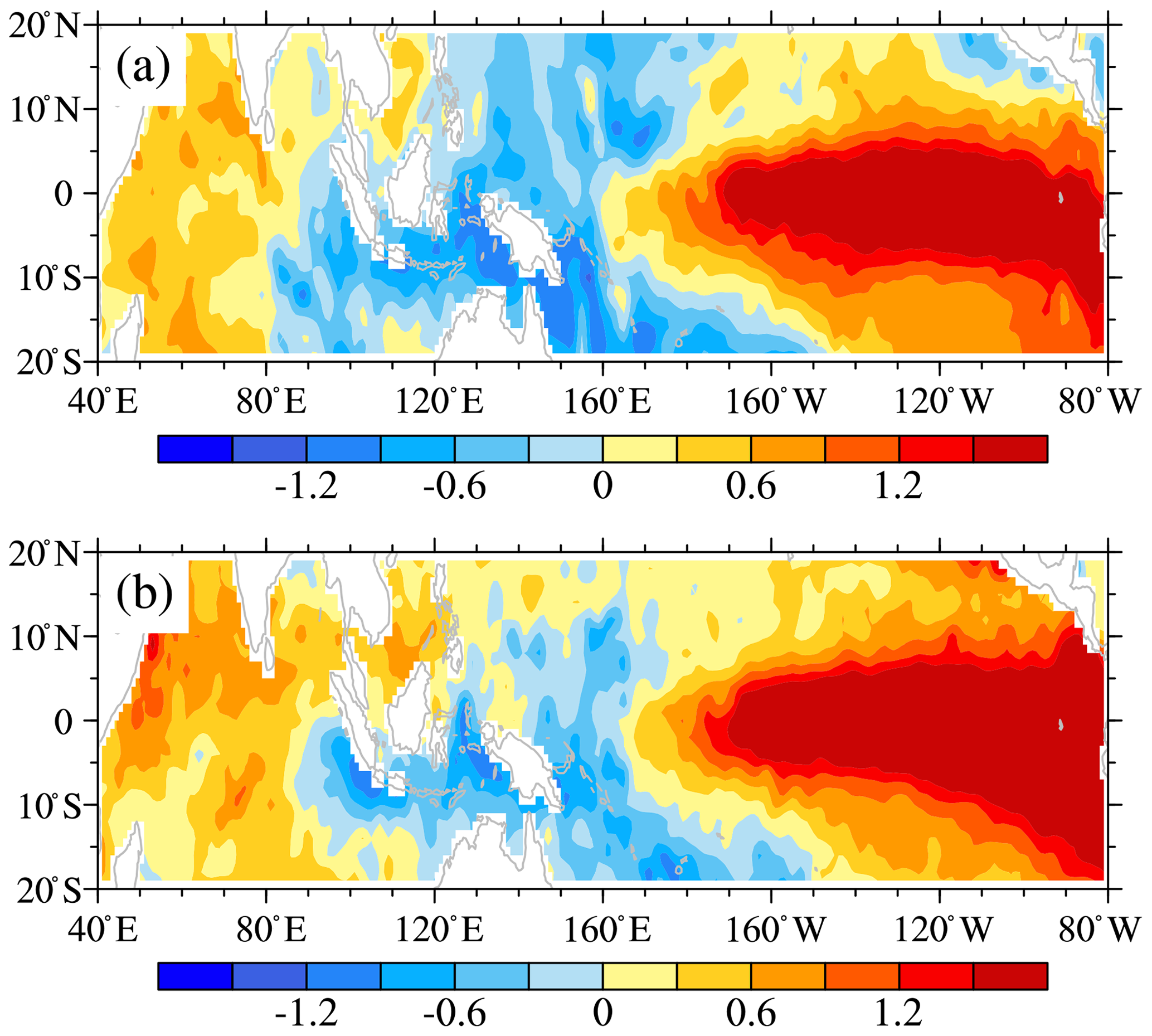
Figure 1Maps of SST anomalies for (a) October 1982 and (b) September 1997 from the HadISST dataset (unit: ∘C). The period from 1981 to 2005 is used to extract the monthly SST climatology.
However, is this spatial pattern of SST anomalies only a special case of a certain year, or is it stable? To answer this question, EOF analysis is performed on the SST anomalies of different seasons over the Pacific–Indian Ocean (20∘ S–20∘ N, 40∘ E–80∘ W) from 1951 to 2005. All these first leading modes in Fig. 2 are well separated from the remaining leading modes, based on the criteria of North et al. (1982), which means that they are less likely to be affected by statistical sampling errors. It can be found that the patterns of summer (June, July and August; Fig. 2b) and autumn (September, October and November; Fig. 2c) display the typical spatial distribution of the PIOAM, with a 46 % and 61 % contribution to total variance, respectively, while the spatial pattern of the PIOAM is not so obvious in spring (March, April and May; Fig. 2a) and winter (December, January and February; Fig. 2d). In general, the PIOAM has stable structure and practical significance, especially in autumn.

Figure 2Spatial patterns of the first leading mode of the (a) spring (March, April and May), (b) summer (June, July and August), (c) autumn (September, October and November) and (d) winter (December, January and February) averaged SST anomalies over the Pacific–Indian Ocean (20∘ S–20∘ N, 40∘ E–80∘ W) calculated from the HadISST dataset (unit: ∘C). The numbers in the upper right corner of each panel indicate the percentage of variance explained by each season.
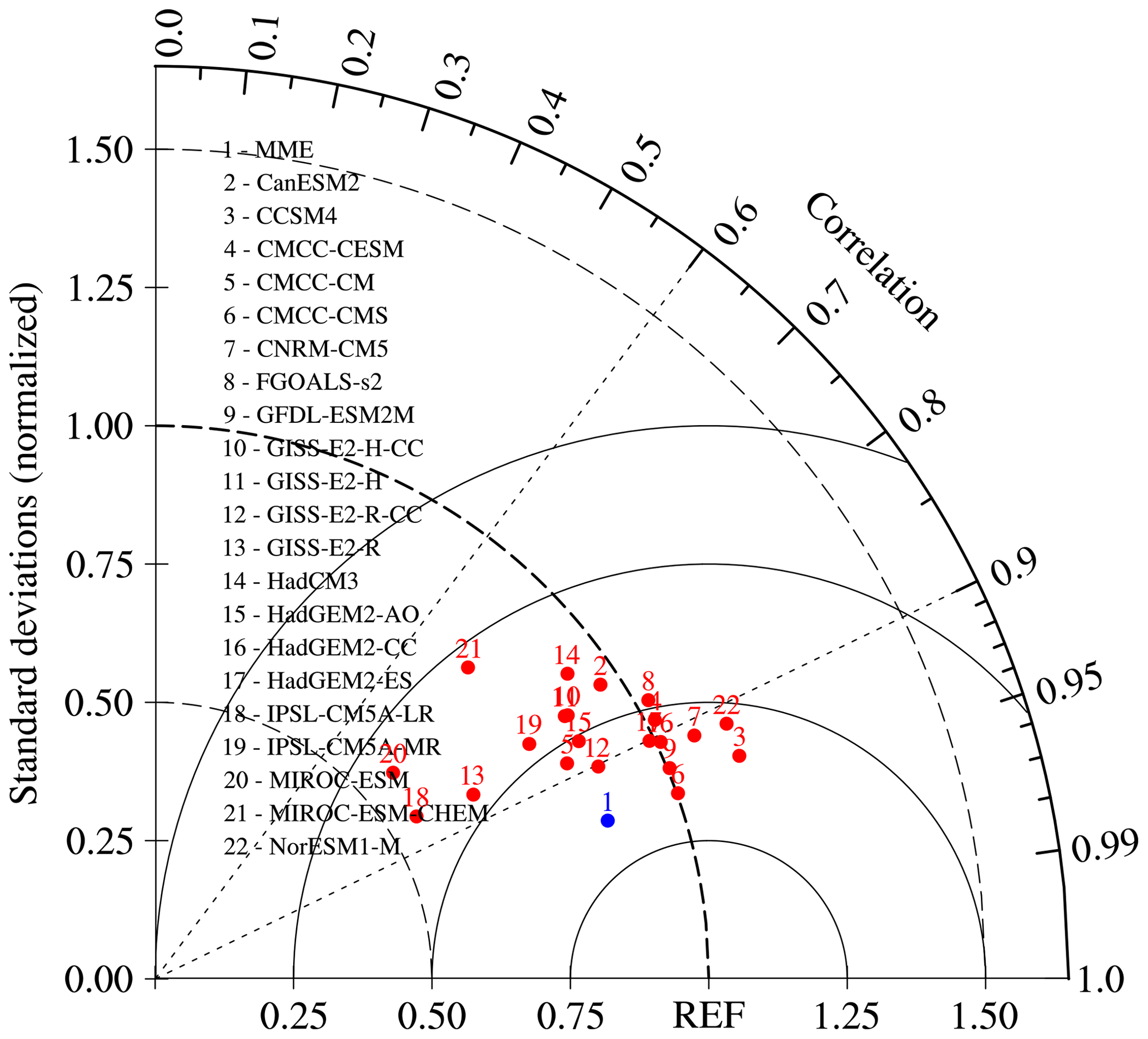
Performing the EOF analysis on the monthly SST anomalies regardless of seasonal differences, Fig. 3 depicts the spatial pattern of the PIOAM in the 21 selected CMIP5 models and their differences compared to the HadISST dataset (Fig. 3a). Figure 3b shows the results of a multi-model ensemble (MME) that represents the mean of the results from all selected models. The PIOAM in the HadISST dataset and CMIP5 models is well separated from the second leading mode, according to the criterion of North et al. (1982). To better and objectively evaluate the capability of each model to simulate the PIOAM, a Taylor diagram (Fig. 4) is also adopted to concisely display the relative information from multiple models, so that the differences among the simulations from all models are revealed clearly (Taylor, 2001; Jiang and Tian, 2013; Yang et al., 2018). According to the HadISST dataset (Fig. 3a), with a 47 % contribution to total variance, the PIOAM has a warm-tongue spatial pattern in the eastern equatorial Pacific Ocean, whereas there is a negative SSTA in the western equatorial Pacific Ocean, which exhibits an obvious ENSO mode in the Pacific Ocean. In addition, there are obvious positive SSTAs in the western Indian Ocean region of the PIOAM, but the SSTAs in the eastern equatorial Indian Ocean region remain positive. Considering that the IOD is defined by the difference between the SSTA in the western equatorial Indian Ocean and that in the eastern equatorial Indian Ocean, this indicates zonal surface heat contrast of the Indian Ocean SSTA. Although it is called a dipole, it is also like a meridional seesaw (Li et al., 2002; Yang et al., 2006). Therefore, the PIOAM can be considered to represent an IOD mode in the Indian Ocean region.
Figure 3 shows that all of these models can generally reproduce the spatial pattern of the PIOAM, yet large discrepancies exist regarding the strength, and the differences between the models are also significant. Except for the contribution to total variance of the PIOAM in CCSM4 and CMCC-CESM being nearly consistent with the HadISST dataset, the variance contribution of the PIOAM in almost all CMIP5 models is lower than in the HadISST dataset, especially CMCC-CM with a contribution to total variance as small as 26 %. In terms of strength, it is apparent that the simulation errors of these models are mainly concentrated in the Pacific Ocean rather than the Indian Ocean. Compared to the HadISST dataset, a majority of models overestimate the strength of the PIOAM in the equatorial east Pacific and central Pacific; only one-seventh of the models (IPSL-CM5A-LR, IPSL-CM5A-MR and MIROC-ESM) underestimate the strength of the PIOAM in the equatorial east Pacific, while the simulation results of HadGEM2-AO and CMCC-CM in the equatorial central Pacific and western Pacific are weak. The simulation errors of the strength of the ENSO-like mode in CCSM4, CMCC-CMS, GFDL-ESM2M and GISS-E2-R-CC are lower than those in other models. For the Indian Ocean, the strengths of the PIOAM in only approximately one-quarter of the models (CanESM2, CMCC-CESM, GISS-E2-H-CC, HadCM3 and HadGEM2-AO) are basically consistent with the HadISST dataset with small simulation errors. Nearly half of the models were smaller for the eastern Indian Ocean, whereas more than half were larger for the western Indian Ocean. In general, the simulation error in the Indian Ocean region is significantly smaller than that in the Pacific region. According to Fig. 4, it is apparent that the root mean square errors (RMSEs) in MIROC-ESM-CHEM, IPSL-CM5A-LR and MIROC-ESM are relatively large, which means that the capabilities of these modes to simulate the strength of the PIOAM are still inadequate, whereas the RMSEs in CCSM4, CMCC-CMS and GFDL-ESM2M are smaller than in other models with better performance. In addition, as shown in Fig. 3b, MME better simulates the amplitude of the PIOAM in the Indian Ocean than most of the selected CMIP5 models with smaller simulation errors, but the amplitude in the equatorial Pacific is larger than that of the HadISST dataset.
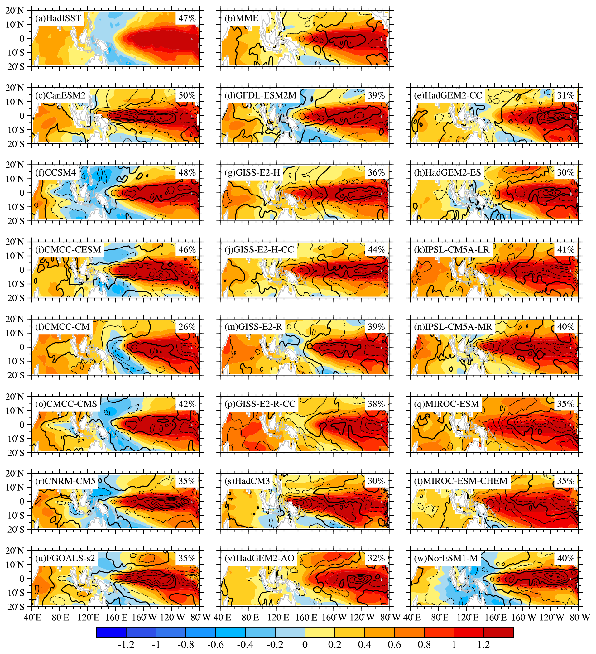
Figure 3PIOAM (shading) and the difference between each model and the HadISST dataset (contours with an interval of 0.3, shown as black bold lines, represent contours with a zero value; dashed contours denote negative values; unit: ∘C). The numbers in the upper right corner of each panel indicate the percentage of variance explained by each model.
As for spatial patterns, the IOD-like mode in the Indian Ocean region can be simulated in almost all models except MIROC-ESM-CHEM. Although all these models reproduce the spatial pattern of the positive SSTA well in the eastern equatorial Pacific, only one-third of the models (CCSM4, CMCC-CM, CMCC-CMS, CNRM-CM5, FGOALS-s2, GFDL-ESM2M and NorESM1-M) successfully simulate the ENSO-like mode with the east–west inverse phase in the Pacific Ocean. In addition, the simulated positive SSTAs in the eastern equatorial Pacific in HadCM3 and MIROC-ESM-CHEM are further south. According to Fig. 4, more than one-third of these models (CCSM4, CMCC-CMS, GFDL-ESM2M etc.) can simulate the spatial pattern of the PIOAM well, and the spatial correlation coefficients between these models and the HadISST dataset are all greater than 0.9, especially CCSM4, which is as high as 0.95. In contrast, the spatial pattern of the PIOAM in MIROC-ESM-CHEM is unsatisfactory with a spatial correlation coefficient of only 0.69. The simulation results of HadCM3 and MIROC-ESM are also relatively poor, and the spatial correlation coefficients with the HadISST dataset are less than 0.8. It can also be learned from Fig. 4 that, for the standard deviation of the PIOAM, very large differences exist among these models. The standard deviations of the PIOAM in IPSL-CM5A-LR, MIROC-ESM and GISS-E2-R-CC are quite different from those of the HadISST dataset, while the simulation results of CMCC-CMS, GFDL-ESM2M and HadGEM2-CC are fairly close to those of the HadISST dataset and have better performance. It is noteworthy that the standard deviations of the PIOAM in more than half of these models are smaller than that of the HadISST dataset, and their differences are large. Although the spatial pattern of the PIOAM in MME is closer to the HadISST dataset and the RMSE is smaller than the vast majority of single models, the standard deviation of the PIOAM in MME is smaller than that of the HadISST dataset.
In general, CCSM4, GFDL-ESM2M and CMCC-CMS have a stronger ability to simulate the PIOAM. In addition, although the MME may not be as good as that of a single model in some specific aspects, overall – considering spatial pattern, standard deviation and RMSE – MME is still superior to most single models.
To further evaluate the differences between these models, Fig. 5 shows the distribution of standard deviations between the CMIP5 models, which clearly reflects the regional differences between the models. It is apparent that the differences are mainly concentrated in the eastern equatorial Pacific. Therefore, the emphasis on simulating the PIOAM is to improve the capability of the model to simulate the eastern Pacific type ENSO.
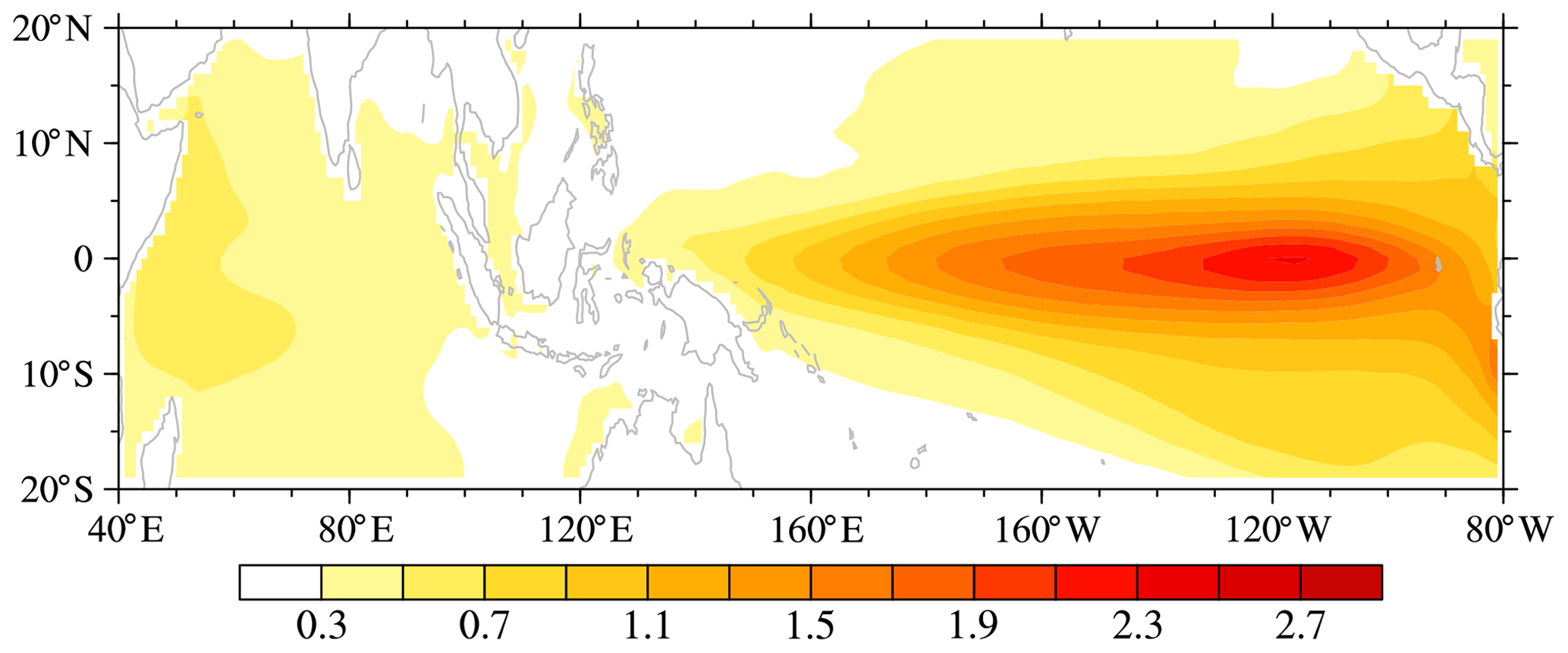
Figure 5The standard deviations of the simulated PIOAM between the 21 selected CMIP5 models (unit: ∘C).
3.2 PIOAM index
3.2.1 Time series
A satisfactory index is needed to describe the PIOAM. It is customary to select the time coefficient (PC1) of the PIOAM as its index. It can be seen from the regression of the monthly SSTA onto the normalized PC1 (Fig. 6a) that the pattern in the Pacific Ocean is similar to ENSO, but positive SST anomalies occur throughout the Indian Ocean, which does not match the typical PIOAM spatial pattern. This is because the ENSO signals in the Pacific Ocean in PC1 are so strong that the signals of the IOD are not fully reflected. The correlation coefficient between PC1 and Niño3.4 index is as high as 0.95. However, obvious negative SST anomalies in the eastern Indian Ocean can be found in the regression map of the monthly SSTA based on the normalized PIOAMI defined in Sect. 2. The correlation coefficient between the PIOAMI and Niño3.4 index is 0.68, indicating the PIOAMI contains more Indian Ocean signals than PC1. In addition, the correlation coefficient between PC1 and the PIOAMI is 0.70, which is far more than the confidence level of 99 %. Therefore, the PIOAMI can describe the mode well because it gives consideration to both the signals in the Pacific Ocean and the signals in the Indian Ocean.

Figure 6Regressions of the monthly SSTA onto the normalized (a) PC1 and (b) PIOAMI for the period from 1951 to 2005 (unit: ∘C). The stippled areas for the SSTA denote the 99 % confidence levels.
In addition, Fig. 7 shows the regressions of the SSTA onto the normalized PC1 and PIOAMI in four seasons. It can also be found that the spatial patterns associated with the PIOAMI (Fig. 7e–h) are closer to the typical spatial pattern of the PIOAM than that associated with PC1 (Fig. 7a–d). Although both the PC1 and the so-called PIOAMI can describe the PIOAM, in the present study we believe that the PIOAMI can better represent the PIOAM than the PC1. Therefore, we chose to only use the PIOAMI to investigate the PIOAM in the following studies, instead of using both indices.

Figure 7Same as Fig. 6 but for the regressions of the (a, e) MAM, (b, f) JJA, (c, g) SON and (d, h) DJF SSTA onto the normalized (a–d) PC1 and (e–h) PIOAMI.
Figure 8 shows the monthly time series of the PIOAMI, POI and IOI from 1951 to 2005. The wavelet analysis of the PIOAMI indicates that the PIOAM has obvious seasonal and interannual variations, as well as interdecadal variations (this feature is omitted). According to Fig. 8, the POI and IOI have the same variation tendency at most times; thus the PIOAMI amplitude is greatly enhanced. However, there are a few cases where the two change in opposing ways, resulting in a much weaker PIOAMI. Moreover, from the time series of the PIOAMI, there is an interannual oscillation of positive and negative phases in the PIOAM, and there is also the phenomenon of the PIOAMI being very weak or not obvious in some years.

Figure 8Time series of the PIOAM index (black), Pacific Ocean index (red) and Indian Ocean index (blue) in the HadISST dataset.
Considering that the PIOAM mainly reaches its peak in autumn (September, October and November), we select the year with significant positive and negative phases of the PIOAM by taking 1 standard deviation as the criterion, and calculate the difference of the autumn PIOAMI between each CMIP5 model and the HadISST dataset (see Fig. 9) to further reveal the simulation of the CMIP5 models on the strength of the PIOAM. As shown by Fig. 9a, the simulated strengths of the PIOAM in the positive phase are underestimated in most models, whereas they are slightly overestimated in less than one-fifth of the models: CCSM4, CMCC-CMS, CNRM-CM5 and GFDL-ESM2M are slightly stronger and very close to the HadISST dataset, especially CCSM4. However, nearly half of the models overestimate the strength of the PIOAM in the negative phase (Fig. 9b), in which the simulation results of CanESM2 and GISS-E2-R are consistent with the HadISST dataset. Although CCSM4 has better performance in simulating the strength of the PIOAM in the positive phase than other models, the simulation error of the negative phase is very large.
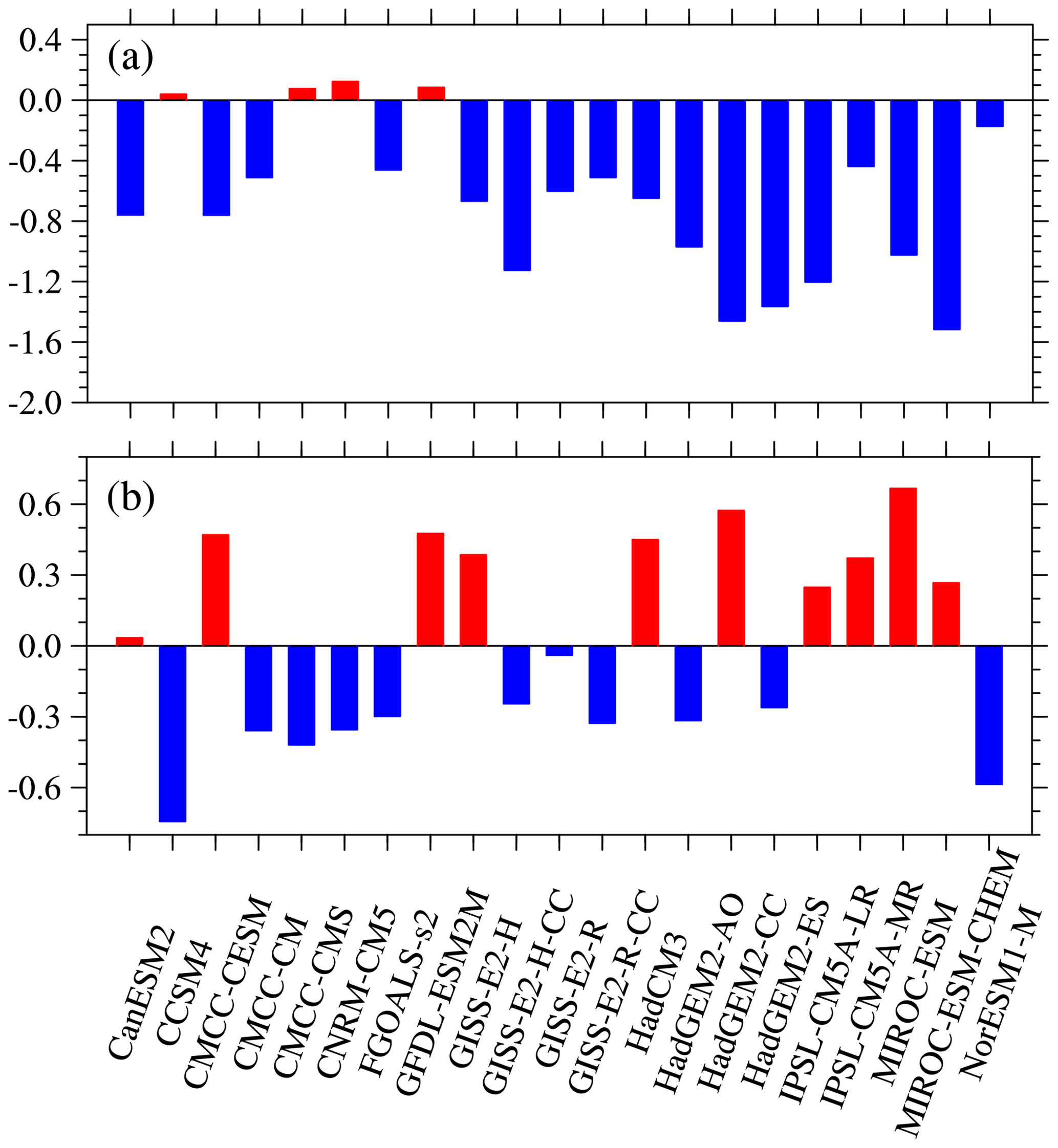
Figure 9Difference in the amplitude of the PIOAMI in the positive phase (a) and negative phase (b) between the CMIP5 models and HadISST dataset.
According to PIOAM positive- and negative-phase years based on the autumn PIOAMI, SSTAs in the tropical Pacific–Indian Ocean in October are composited to obtain the spatial pattern of SSTAs in the PIOAM positive and negative phases. It is clear in Fig. 10 that the SSTAs in the Pacific–Indian Ocean in both the MME of CMIP5 models and the HadISST dataset present patterns with a tripole structure, where the Indian Ocean is represented by the IOD-like mode and the Pacific Ocean by the ENSO-like mode, which again demonstrates the authenticity of the PIOAM and the rationality of the PIOAMI used in this article.
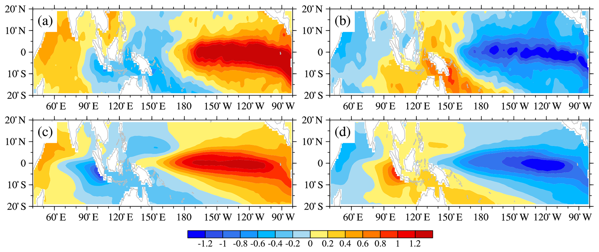
Figure 10The tropical Pacific–Indian Ocean SSTAs of the PIOAM positive (a, c) and negative (b, d) phase in October in the HadISST dataset (a, b) and the MME of CMIP5 models (c, d) (unit: ∘C).
3.2.2 Interannual variation of the PIOAM
To evaluate the ability of these CMIP5 models to simulate the interannual variation of the PIOAM, Fig. 11 shows the ratios of the standard deviation of the IOI, POI and PIOAMI in autumn in each model to those in the HadISST dataset. The closer the ratio is to 1, the better the ability to simulate interannual variation. It can be found that the difference in the simulation results of the interannual variation of the PIOAMI among these models is smaller compared to the IOI and POI. The simulation results of CCSM4, GISS-E2-R and FGOALS-s2 are almost consistent with the HadISST dataset, indicating that these three models have relatively strong capabilities to simulate the interannual variation of the PIOAM. Except for NorESM1-M overestimating the interannual variation of the PIOAM, the simulation results in most of the models being weak, especially MIROC-ESM, which leads to MME underestimating the interannual variation of the PIOAM compared to the HadISST dataset. In addition, the interannual variations of the IOI in GFDL-ESM2M, GISS-E2-R-CC and CMCC-CM are better than other models, whereas the simulation results are underestimated in most models. In contrast to the IOI, the vast majority of models overestimate the interannual variations of the POI, and the simulated interannual variations of the POI in only three models (IPSL-CM5A-MR, CMCC-CESM and IPSL-CM5A-LR) are weaker than the HadISST dataset. Based on the above analysis, it is apparent that the interannual variation of the PIOAMI is more closely related to the IOI than POI, and the interannual variation of the PIOAM in autumn can be measured by CCSM4, GISS-E2-R and FGOALS-s2.
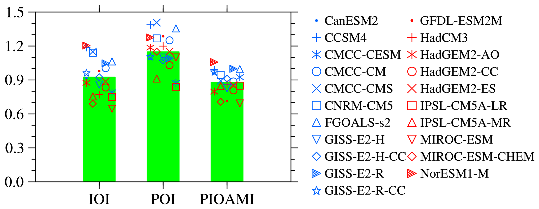
Figure 11Ratios of standard deviation of the autumn IOI, POI and PIOAMI in each model to those in the HadISST dataset. Green bar represents the MME of the corresponding index.
3.2.3 The relationship of the PIOAM with ENSO and the IOD
The lag–lead correlation analysis between the PIOAMI and the Niño3.4 index derived from the HadISST dataset shows that the PIOAM has a close correlation with the ENSO mode in the same period and 1 month lagging with the correlation coefficient of 0.68 (Fig. 12a). In addition, the PIOAM and IOD also have a close correlation in the same period, with a correlation coefficient of 0.73 (Fig. 12b), indicating that the PIOAM can reflect the activities of ENSO in the Pacific Ocean and the IOD in the Indian Ocean to a considerable extent. It should be noted that the IOD index used in this research is based upon the definition of Saji et al. (1999), i.e., the difference in SSTA between the tropical western Indian Ocean (50–70∘ E, 10∘ S–10∘ N) and the tropical southeastern Indian Ocean (90–110∘ E, 10–0∘ S). In these CMIP5 models, more than one-half of the models successfully reproduce the maximum correlation between the PIOAM and ENSO in the same period. The correlation coefficients of the PIOAMI and the Niño3.4 index in HadGEM2-AO and HadGEM2-ES are both 0.68, which is consistent with the HadISST dataset, and the correlation coefficients of FGOALS-s2, GISS-E2-H and GISS-E2-H-CC are 0.69, 0.69 and 0.70, respectively. However, the correlation coefficients of MIROC-ESM and MIROC-ESM-CHEM are only 0.37 and 0.30, which are significantly different from the results of the HadISST dataset and other models, indicating that the two models cannot simulate the close relationship between the PIOAM and ENSO well. In addition, the correlation coefficient of the PIOAMI and the Niño3.4 index in MME is 0.66, which is slightly lower than the HadISST dataset but shows the close contemporaneity correlation between the PIOAM and ENSO; the overall change of the correlation coefficient series is very close to the HadISST dataset.
For the relationship between the PIOAM and IOD, it is apparent from the HadISST dataset in Fig. 12b that the PIOAM and IOD show obvious close correlation in the same period, and the correlation coefficient is as high as 0.73. It is satisfactory that all selected CMIP5 models successfully reproduce the correlation between the PIOAM and IOD in the same period, but the simulation results in more than half of them are underestimated. Among these models, the simulation results of HadGEM2-ES and GIS-E2-R-CC are basically consistent with the HadISST dataset, which shows that the two models have stronger capability to simulate the relationship between the PIOAM and IOD.
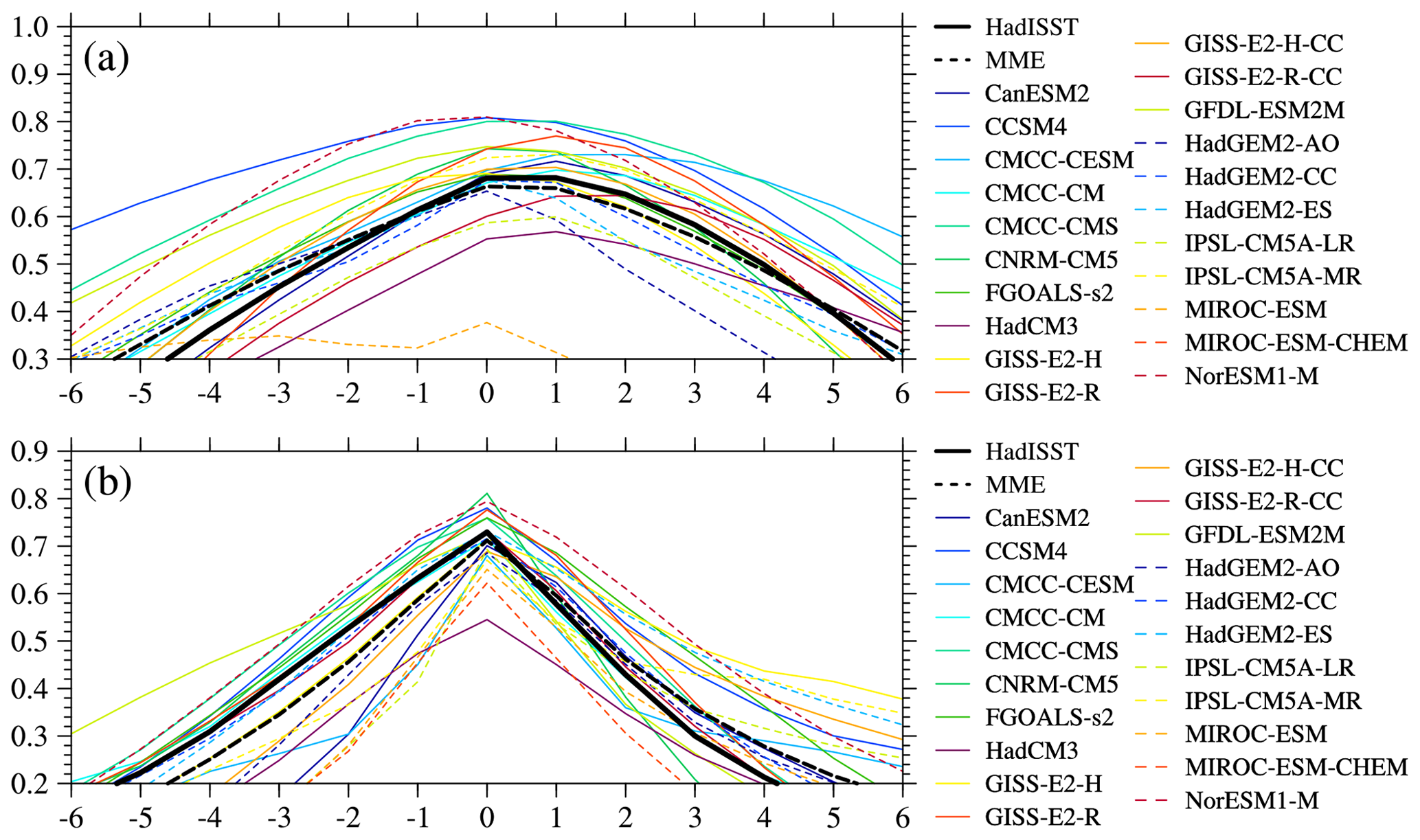
Figure 12The lag–lead correlation coefficient of the PIOAMI with the Niño3.4 index (a) and IOD index (b). Ordinate represents the correlation coefficient, and abscissa is the lag in months: positive (negative) for the Niño3.4 index or IOD index (PIOAMI) leading PIOAMI (Niño3.4 index or IOD index).
Based on the HadISST dataset from 1951 to 2005, the Pacific–Indian Ocean associated mode proposed by Yang and Li (2005) is evaluated for 21 CMIP5 models. This research provides a relatively comprehensive evaluation of the spatial pattern, the interannual variation and the relationship with ENSO and the IOD of the PIOAM in the selected CMIP5 models. The main conclusions are as follows.
With a 47 % contribution to total variance, the spatial pattern of the PIOAM in the eastern equatorial Pacific Ocean is a warm tongue, whereas there is a negative SSTA in the western equatorial Pacific Ocean that exhibits an obvious ENSO mode in the Pacific Ocean. In addition, the PIOAM presents an IOD mode in the Indian Ocean. The variance contributions of the PIOAM in almost all CMIP5 models are smaller than that in the HadISST dataset. The simulation errors and differences among these models are mainly concentrated in the Pacific Ocean, rather than the Indian Ocean, and a majority of models overestimate the strength of the PIOAM in the equatorial east Pacific and central Pacific. Although all these models reproduce the spatial pattern of the positive SSTA in the eastern equatorial Pacific well, only one-third of the models (CCSM4, CMCC-CM, CMCC-CMS, CNRM-CM5, FGOALS-s2, GFDL-ESM2M and NorESM1-M) successfully simulate the ENSO mode with the east–west inverse phase in the Pacific Ocean. In general, CCSM4, GFDL-ESM2M and CMCC-CMS have a stronger capability to simulate the PIOAM than the other models.
The PIOAM is very weak or not obvious in some years and has obvious seasonal and interannual variations, as well as interdecadal variations. The simulated strengths of the PIOAM in the positive phase are underestimated in most models; less than one-fifth of the models (CCSM4, CMCC-CMS, CNRM-CM5 and GFDL-ESM2M) are slightly stronger, and very close to the HadISST dataset, especially CCSM4. The interannual variation of the PIOAM in CCSM4, GISS-E2-R and FGOALS-s2 is almost consistent with the HadISST dataset. Except for NorESM1-M overestimating the interannual variation of the PIOAM, the simulation results in most models being weak, especially MIROC-ESM. The interannual variation of the PIOAM in autumn can be measured by CCSM4, GISS-E2-R and FGOALS-s2. The PIOAM are able to reflect well the activities of ENSO in the Pacific Ocean and the IOD in the Indian Ocean to a considerable extent with a close correlation to ENSO and the IOD for the same period, as well as 1 month in advance with ENSO.
It is undoubtedly difficult to directly find the factors that influence the model to simulate the PIOAM. The simulation results of model families – such as CMCC, IPSL, MIROC, GISS and HadGEM2 – provide clues and comparative data with which to find the possible reasons for simulation differences. However, in-depth analysis supported by a large number of models, or by dedicated experiments, is necessary.
Yang et al. (2006) found that only considering the ENSO in the Pacific cannot entirely explain the influence of SSTA on climate variation and suggested that, to provide better scientific explanation for short-term climate prediction, the PIOAM and its influence should be considered and investigated. In addition, a review article by Cai et al. (2019) provides the first comprehensive review and summary of the current research advances in the interaction between the tropical Pacific, Indian and Atlantic Ocean climate systems, and they pointed out that an in-depth understanding of the dynamic mechanisms of intertropical basin interactions is an important way to improve the ability of seasonal to decadal climate prediction. Therefore, evaluating and improving the capability of current climate models to simulate the PIOAM and even the tropical Pacific, Indian and Atlantic Ocean climate systems contribute to obtaining accurate climate change predictions. In addition, improving the level of climate prediction is not only helpful for grasping the changes in the ocean environment of the Pacific–Indian Ocean but also propitious for improving the ability of prediction and assessment of ocean waves and wind energy (Zheng and Li, 2015, 2017).
The CMIP5 data are available at https://esgf-node.llnl.gov/search/cmip5/ (last access: 12 April 2020, ESGF, 2020). The sea surface temperature data are available at https://www.metoffice.gov.uk/hadobs/hadisst/data/download.html (last access: 12 April 2020, MetOffice, 2020).
XL and WS conceived the idea and designed the structure of this paper; MY performed the experiments; MY, CZ and JZ analyzed the data; and MY wrote the paper.
The authors declare that they have no conflict of interest.
Two anonymous reviewers provided careful and constructive comments on the submitted manuscript, which helped improve this article. The first author thanks Handling Topic Editor David Stevens and Handling Executive Editor John M. Huthnance for their help in finding excellent reviewers.
This research has been jointly supported by the National Natural Science Foundation of China (grant nos. 4160501, 41490642 and 41520104008) and the “Double First-Class” construction guidance project of the National University of Defense Technology (project no. ZXBJGB02).
This paper was edited by David Stevens and reviewed by Ian Watterson and two anonymous referees.
Annamalai, H., Xie, S. P., Mccreary, J. P., and Murtugudde, R.: Impact of Indian Ocean Sea Surface Temperature on Developing El Niño, J. Climate, 18, 302–319, https://doi.org/10.1175/jcli-3268.1, 2005.
Bjerknes, J.: A possible response of the atmospheric Hadley circulation to equatorial anomalies of ocean temperature, Tellus, 18, 820–829, https://doi.org/10.3402/tellusa.v18i4.9712, 1966.
Bjerknes, J.: Atmospheric teleconnections from the equatodal Pacific, Mon. Weather Rev., 97, 163–172, https://doi.org/10.1175/1520-0493(1969)097<0163:ATFTEP>2.3.CO;2, 1969.
Cai, W., Hendon, H. H., and Meyers, G.: Indian Ocean dipolelike variability in the CSIRO Mark 3 coupled climate model, J. Climate, 18, 1449–1468, https://doi.org/10.1175/jcli3332.1, 2005.
Cai, W., Wu, L., Lengaigne, M., Li, T., McGregor, S., Kug, J.-S., Yu, J.-Y., Stuecker, M. F., Santoso, A., Li, X., Ham, Y.-G., Chikamoto, Y., Ng, B., McPhaden, M. J., Du, Y., Dommenget, D., Jia, F., Kajtar, J. B., Keenlyside, N., Lin, X., Luo, J.-J., Martín-Rey, M., Ruprich-Robert, Y., Wang, G., Xie, S.-P., Yang, Y., Kang, S. M., Choi, J.-Y., Gan, B., Kim, G.-I., Kim, C.-E., Kim, S., Kim, J.-H., and Chang, P.: Pantropical climate interactions, Science, 363, eaav4236, https://doi.org/10.1126/science.aav4236, 2019.
Chen, D.: Indo-Pacific Tripole: An intrinsic mode of tropical climate variability, Advances in Geosciences, 24, 1–18, https://doi.org/10.1142/9789814355353_0001, 2011.
Chen, D. and Cane, M. A.: El Niño prediction and predictability, J. Comput. Phys., 227, 3625–3640, https://doi.org/10.1016/j.jcp.2007.05.014, 2008.
ESGF (Earth System Grid Federation): CMIP5 project data, available at: https://esgf-node.llnl.gov/search/cmip5/ (last access: 12 April 2020), 2020.
Guo, Y. F.: Numerical simulation of the 1999 Yangtze River valley heavy rainfall including sensitivity experiments with different anomalies, Adv. Atmos. Sci., 19, 391–404, https://doi.org/10.1007/BF02915677, 2004.
Guo, Y. F., Zhao, Y., and Wang, J.: Numerical simulation of the relationships between the 1998 Yangtze River valley floods and SST anomalies, Adv. Atmos. Sci., 19, 391–404, https://doi.org/10.1007/s00376-002-0074-0, 2002.
Huang, B. H. and Kinter, J. L.: Interannual variability in the tropical Indian Ocean, J. Geophys. Res., 107, 3199, https://doi.org/10.1029/2001JC001278, 2002.
Jiang, D. B. and Tian, Z. P.: East Asian monsoon change for the 21st century: results of CMIP3 and CMIP5 models, Chinese Sci. Bull., 58, 1427–1435, https://doi.org/10.1007/s11434-012-5533-0, 2013.
Jin, F. F.: An equatorial ocean recharge paradigm for ENSO. Part I: Conceptual model, J. Atmos. Sci., 54, 811–829, https://doi.org/10.1175/1520-0469(1997)054<0811:AEORPF>2.0.CO;2, 1997.
Ju, J. H., Chen, L. L., and Li, C. Y.: The preliminary research of Pacific-Indian Ocean sea surface tempertature anomaly mode and the definition of its index, J. Trop. Meteorol., 20, 617–624, 2004 (in Chinese).
Klein, S. A. and Soden, B. J.: Remote sea surface temperature variation during ENSO: evidence for a tropical atmospheric bridge, J. Climate, 12, 917–932, https://doi.org/10.1175/1520-0442(1999)012<0917:RSSTVD>2.0.CO;2, 1999.
Li, C. Y.: Interaction between anomalous winter monsoon in East Asia and El Niño events, Adv. Atmos. Sci., 7, 36–46, https://doi.org/10.1007/bf02919166, 1990.
Li, C. Y.: A Further Study of the Essence of ENSO, Climate and Environmental Research, 7, 160–174, 2002 (in Chinese).
Li, C. Y. and Mu, M. Q.: El Niño occurrence and sub-surface ocean temperature anomalies in the Pacific warm pool, Chinese Journal of Atmospheric Sciences, 23, 513–521, 1999 (in Chinese).
Li, C. Y. and Mu, M. Q.: Relationship between East Asian winter monsoon, warm pool situation and ENSO cycle, Chin. Sci. Bull., 45, 1448–1455, https://doi.org/10.1007/BF02898885, 2000.
Li, C. Y. and Mu, M. Q.: The influence of the Indian Ocean dipole on atmospheric circulation and climate, Adv. Atmos. Sci., 18, 831–843, https://doi.org/10.1007/BF03403506, 2001.
Li, C. Y., Mu, M. Q., and Pan, J.: Indian Ocean temperature dipole and SSTA in the equatorial Pacific Ocean, Chin. Sci. Bull., 47, 236–239, https://doi.org/10.1360/02tb9056, 2002.
Li, C. Y., Mu, M., Zhou, G. Q., and Yang, H.: Mechanism and prediction studies of the ENSO, Chinese Journal of Atmospheric Sciences, 32, 761–781, 2008 (in Chinese).
Li, C. Y., Li, X., Yang, H., Pan, J., and Li, G.: Tropical Pacific-Indian Ocean Associated Mode and Its Climatic Impacts, Chinese Journal of Atmospheric Sciences, 42, 505–523, 2018 (in Chinese).
Li, T., Wang, B., Chang, C. P., and Zhang, Y.: A theory for the Indian Ocean dipole-zonal mode, J. Atmos. Sci., 60, 2119–2135, https://doi.org/10.1175/1520-0469(2003)060<2119:ATFTIO>2.0.CO;2, 2003.
Li, X., Li, C. Y., Tan, Y. K., Zhang, R., and Li, G.: Tropical Pacific-Indian Ocean thermocline temperature associated anomaly mode and its evolvement, Chinese Journal of Geophysics–Chinese Edition, 56, 3270–3284, https://doi.org/10.6038/cjg20131005, 2013 (in Chinese).
Li, X. and Li, C. Y.: The tropical pacific–indian ocean associated mode simulated by licom2.0, Adv. Atmos. Sci., 34, 1426–1436, https://doi.org/10.1007/s00376-017-6176-5, 2017.
Lian, T., Chen, D. K., Tang, Y. M., and Jin, B. G.: A theoretical investigation of the tropical Indo-Pacific tripole mode, Sci. China Earth Sci., 57, 174–188, https://doi.org/10.1007/s11430-013-4762-7, 2014.
Liu, H., Lin, P., Yu, Y., and Zhang, X.: The baseline evaluation of LASG/IAP Climate system Ocean Model (LICOM) version 2, Acta. Meteorol. Sin., 26, 318–329, https://doi.org/10.1007/s13351-012-0305-y, 2012.
MetOffice: HadISST1 Data, available at: https://www.metoffice.gov.uk/hadobs/hadisst/data/download.html, last access: 12 April 2020.
Mu, M. and Duan, W. S.: A new approach to studying ENSO predictability: Conditional nonlinear optimal perturbation, Chin. Sci. Bull., 48, 1045–1047, https://doi.org/10.1007/BF03184224, 2003.
Mu, M., Duan, W. S., and Wang, B.: Season-dependent dynamics of nonlinear optimal error growth and El Niño-Southern Oscillation predictability in a theoretical model, J. Geophys. Res., 112, D10113, https://doi.org/10.1029/2005JD006981, 2007.
North, G. R., Bell, T. L., Cahalan, R. F., and Moeng, F. J.: Sampling errors in the estimation of empirical orthogonal functions, Mon. Weather Rev., 110, 699–706, https://doi.org/10.1175/1520-0493(1982)110<0699:SEITEO>2.0.CO;2, 1982.
Philander, S. G. H., Yamagata, T., and Pacanowski, R. C.: Unstable Air-Sea Interactions in the Tropics, J. Atmos. Sci., 41, 604–613, https://doi.org/10.1175/1520-0469(1984)041<0604:UASIIT>2.0.CO;2, 1984.
Rao, S. A., Masson, S., Luo, J. J., Behera, S. K., and Yamagata, T.: Termination of indian ocean dipole events in a coupled general circulation model, J. Climate, 20, 3018–3035, https://doi.org/10.1175/JCLI4164.1, 2007.
Rasmusson, E. M. and Wallace, J. M.: Meteorological aspects of the El Niño/Southern Oscillation, Science, 222, 1195–1202, https://doi.org/10.1126/science.222.4629.1195, 1983.
Rayner, N. A., Parker, D. E., Horton, E. B., Folland, C. K., Alexander, L. V., Rowell, D. P., Kent, E. C., and Kaplan, A.: Global analyses of sea surface temperature, sea ice, and night marine air temperature since the late nineteenth century, J. Geophys. Res., 108, 4407, https://doi.org/10.1029/2002JD002670, 2003.
Ropelewski, C. F. and Halpert, M. S.: Global and regional scale precipitation patterns associated with the El Niño/southern Oscillation, Mon. Weather Rev., 115, 1606–1626, https://doi.org/10.1175/1520-0493(1987)115<1606:GARSPP>2.0.CO;2, 1987.
Saji, N. H. and Yamagata, T.: Possible impacts of Indian Ocean dipole mode events on global climate, Clim. Res., 25, 151–169, https://doi.org/10.3354/cr025151, 2003.
Saji, N. H., Coswami, B. N., Vinayachandran, P. N., and Yamagata, T.: A dipole in the tropical Indian Ocean, Nature, 401, 360–363, https://doi.org/10.1038/43854, 1999.
Shen, X. S., Kimoto, M., Sumi, A., Numaguti, A., and Matsumoto, J.: Simulation of the 1998 East Asian Summer Monsoon by the CCSR/NIES AGCM, J. Meteorol. Soc. Jpn., 79, 741–757, https://doi.org/10.2151/jmsj.79.741, 2001.
Suarez, M. J. and Schopf, P. S.: A delayed action oscillator for ENSO, J. Atmos. Sci., 45, 3283–3287, https://doi.org/10.1175/1520-0469(1988)045<3283:ADAOFE>2.0.CO;2, 1988.
Taylor, K. E.: Summarizing multiple aspects of model performance in a single diagram, J. Geophys. Res., 106, 7183–7192, https://doi.org/10.1029/2000jd900719, 2001.
Ueda, H. and Matsumoto, J.: A possible triggering process of East–West asymmetric anomalies over the Indian Ocean in relation to 1997/98 El Niño, J. Meteorol. Soc. Jpn., 78, 803–818, https://doi.org/10.2151/jmsj1965.78.6_803, 2000.
Webster, P. J. and Yang, S.: Monsoon and ENSO: Selectively interactive systems, Q. J. Roy. Meteor. Soc., 118, 877–926, https://doi.org/10.1002/qj.49711850705, 1992.
Webster, P. J., Moore, A. M., Loschnigg, J. P., and Leben R. R.: Coupled ocean-atmosphere dynamics in the Indian Ocean during 1997–98, Nature, 401, 356–360, https://doi.org/10.1038/43848, 1999.
Wang, X. and Wang, C. Z.: Different impacts of various El Niño events on the Indian Ocean Dipole, Clim. Dynam., 42, 991–1005, https://doi.org/10.1175/JCLI-D-12-00638.1, 2014.
Wyrtki, K.: El Niño-The Dynamic Response of the Equatorial Pacific Ocean to Atmospheric Forcing, J. Phys. Oceanogr., 5, 572–584, https://doi.org/10.1175/1520-0485(1975)005<0572:entdro>2.0.CO;2, 1975.
Yang, H. and Li, C. Y.: Effect of the Tropical Pacific-Indian Ocean Temperature Anomaly Mode on the South Asia High, Chinese Journal of Atmospheric Science, 29, 99–110, 2005 (in Chinese).
Yang, H., Jia, X. L., and Li, C. Y.: The tropical Pacific-Indian Ocean temperature anomaly mode and its effect, Chin. Sci. Bull., 51, 2878–2884, https://doi.org/10.1007/s11434-006-2199-5, 2006.
Yang, M., Li, X., Zuo, R., Chen, X., and Wang, L.: Climatology and Interannual Variability of Winter North Pacific Storm Track in CMIP5 Models, Atmosphere, 9, 79, https://doi.org/10.3390/atmos9030079, 2018.
Yu, L. S. and Rienecker, M. M.: Mechanisms for the Indian Ocean warming during the 1997-98 El Niño, Geophys. Res. Lett., 26, 735–738, https://doi.org/10.1029/1999GL900072, 1999.
Zheng, C. W. and Li, C. Y.: Variation of the wave energy and significant wave height in the China Sea and adjacent waters, Renew. Sust. Energ. Rev., 43, 381–387, https://doi.org/10.1016/j.rser.2014.11.001, 2015.
Zheng, C. W. and Li, C. Y.: Propagation characteristic and intraseasonal oscillation of the swell energy of the Indian Ocean, Appl. Energ., 197, 342–353, https://doi.org/10.1016/j.apenergy.2017.04.052, 2017.
Zheng, F., Zhu, J., and Zhang, R. H.: The impact of altimetry data on ENSO ensemble initializations and predictions, Geophys. Res. Lett., 34, L13611, https://doi.org/10.1029/2007gl030451, 2007.
Zheng, X. T., Xie, S. P., Du, Y., Liu, L., Huang, G., and Liu, Q.: Indian Ocean Dipole Response to Global Warming in the CMIP5 Multimodel Ensemble, J. Climate, 26, 6067–6080, https://doi.org/10.1175/JCLI-D-12-00638.1, 2013.
Zhou, G. Q. and Zeng, Q. C.: Predictions of ENSO with a coupled atmosphere–ocean general circulation model, Adv. Atmos. Sci., 18, 587–603, https://doi.org/10.1007/s00376-001-0047-8, 2001.