the Creative Commons Attribution 4.0 License.
the Creative Commons Attribution 4.0 License.
 | 24 Jan 2020
Temporal evolution of temperatures in the Red Sea and the Gulf of Aden based on in situ observations (1958–2017)
Miguel Agulles
Gabriel Jordà
Burt Jones
Susana Agustí
Carlos M. Duarte
The Red Sea holds one of the most diverse marine ecosystems in the world, although fragile and vulnerable to ocean warming. Several studies have analysed the spatio-temporal evolution of temperature in the Red Sea using satellite data, thus focusing only on the surface layer and covering the last ∼30 years. To better understand the long-term variability and trends of temperature in the whole water column, we produce a 3-D gridded temperature product (TEMPERSEA) for the period 1958–2017, based on a large number of in situ observations, covering the Red Sea and the Gulf of Aden. After a specific quality control, a mapping algorithm based on optimal interpolation have been applied to homogenize the data. Also, an estimate of the uncertainties of the product has been generated. The calibration of the algorithm and the uncertainty computation has been done through sensitivity experiments based on synthetic data from a realistic numerical simulation.
TEMPERSEA has been compared to satellite observations of sea surface temperature for the period 1981–2017, showing good agreement especially in those periods when a reasonable number of observations were available. Also, very good agreement has been found between air temperatures and reconstructed sea temperatures in the upper 100 m for the whole period 1958–2017, enhancing confidence in the quality of the product.
The product has been used to characterize the spatio-temporal variability of the temperature field in the Red Sea and the Gulf of Aden at different timescales (seasonal, interannual and multidecadal). Clear differences have been found between the two regions suggesting that the Red Sea variability is mainly driven by air–sea interactions, while in the Gulf of Aden the lateral advection of water plays a relevant role. Regarding long-term evolution, our results show only positive trends above 40 m depth, with maximum trends of 0.045 + 0.016 ∘C decade−1 at 15 m, and the largest negative trends at 125 m ( ∘C decade−1). Multidecadal variations have a strong impact on the trend computation and restricting them to the last 30–40 years of data can bias high the trend estimates.
- Article
(9877 KB) - Full-text XML
-
Supplement
(212 KB) - BibTeX
- EndNote


The Red Sea is a narrow basin, meridionally elongated (2250 km), lying between the African and the Asian continental shelves, and extending from 12.5 to 30∘ N with an average width of 220 km (Fig. 1). It is a semi-enclosed basin connected to the Indian Ocean through the Bab-al-Mandeb strait, with a still depth of 137 m (Werner and Lange, 1975), at the south and to the Mediterranean Sea through the Suez Canal at the north. The bathymetry is highly irregular along the basin, with a relatively shallow mean depth (524 m; Patzert, 1974) but with maximum recorded depths of almost 3000 m. At its northern end, it bifurcates into two gulfs, the Gulf of Suez in the west with an average depth of 40 m and the Gulf of Aqaba in the east with depths exceeding 1800 m (Neumann and McGill, 1961).
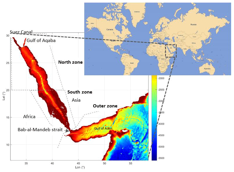
Figure 1Domain and bathymetry of the region included in the TEMPERSEA product. The three zones used in the presentation of results (North zone, South zone and Outer zone) are identified by grey lines. (data source: https://www.gebco.net/data_and_products/gridded_bathymetry_data, last access: March 2018).
The transport through the Suez Canal, which connects the Mediterranean Sea with the Gulf of Suez and the Red Sea, is relatively small, and therefore the only significant connection between the Red Sea and the global ocean is the Bab-al-Mandeb strait (Sofianos and Jhons, 2015). There, a two layer system is established in which relatively fresh and cold waters flow from the Indian Ocean into the Red Sea in the upper layer, while saltier and warmer waters flow outside in the lower layer. Due to its arid setting, the Red Sea experiences one of the largest evaporation rates in the world, which in combination with its semi-enclosed nature leads to high salinities across the whole basin (Sofianos and Jhons, 2015). The hydrodynamic characteristics are strongly influenced by the wind forcing with different seasonality. The seasonal winds blow south-eastwards in the northern part of the basin through the whole year, but in the southern region the winds reverse form north-westerly in summer to south-easterly in winter under the influence of the two distinct phases of the Arabian monsoon, (Patzert, 1974; Sofianos and Jhons, 2015).
The Red Sea holds one of the most diverse marine ecosystems in the world, although fragile and vulnerable to ocean warming (Thorne et al., 2010). Water temperature plays a key role in ecosystem evolution, which is usually adapted to the environmental thermal range. Marine species respond to ocean warming by shifting their distribution poleward and advancing their phenology (Poloczanska et al., 2016). While parts of the ocean may be warming gradually, others may experience rapid fluctuations, inducing more significant impacts on biodiversity. Impacts of warming are likely to be greatest in semi-enclosed seas, which tend to support warming rates higher than the global ones (Lima and Wethey, 2012), as documented for the Red Sea (Chaidez et al., 2017).
Several recent studies have analysed the spatio-temporal evolution of temperature in the Red Sea using satellite data from AVHRR (Advanced Very High-Resolution Radiometer), thus focusing only on the surface layer and covering from early 1980s onwards. Those studies have identified a warming trend with values ranging from 0.17 to 0.45 ∘C decade−1 across the basin for the period 1982–2015 (Chaidez et al., 2017). Also, sea surface temperature exhibits a strong interannual variability (Eladawy et al., 2017) which is mainly driven by the air temperature (Raitsos et al., 2011). However, these studies are limited to ∼30 years due to the observational period of remote data. Also, although the evolution of surface conditions is very relevant, the temperature variability in the whole water column has effects on marine biota (Bongaerts et al., 2010), so products based on depth-resolving in situ observations better reflect the thermal regime across the ecosystem than sea surface trends alone.
Global hydrographic products like EN4 (Good et al., 2013) or ISHII (Ishii and Kimoto, 2009) that interpolate in situ observations to create a monthly 3-D product for the last decades are available. However, those products have low spatial resolution (∼1∘) and the quality controls applied are not region specific, which cast doubts on their accuracy in the narrow Red Sea. In order to overcome the limitations satellite products and global hydrographic products have, and to be able to characterize the spatio-temporal variability of the 3-D temperature field to inform research on the thermal ecology and variability of Red Sea ecosystems, a dedicated regional observational product is required.
Here we produce a gridded temperature product for the period 1958–2017 at monthly resolution as a resource to describe the evolution of the Red Sea temperature during the last 6 decades and underpin research on the impacts of ocean warming across the Red Sea. The product covers the Red Sea and the Gulf of Aden with a spatial resolution of 0.25∘ × 0.25∘. This product is based on the assimilation and reanalysis of a large number of in situ observations collected in the region. After a specific quality control, a mapping algorithm has been applied to homogenize the data. Also, an estimate of the accuracy of the product has been generated to accurately define the uncertainties of the product. We then use the product to characterize the seasonal, interannual and multidecadal variability of the 3-D temperature field in the Red Sea and the Gulf of Aden.
2.1 In situ data
In situ potential temperature observations were obtained from two databases. The first one is CORA (Cabanes et al., 2013), a delayed mode product (the April release corresponds to profiles dated up to June of the n−1 year) designed to feed global reanalyses. CORA covers the global ocean from 1950 to 2016 and integrates quality-controlled historical profiles from several data collections (Argo, GOSUD, OceanSITES and World Ocean Database). The details of this database can be found at http://www.coriolis.eu.org/Science2/Global-Ocean/CORA (last access: October 2018), and it is freely delivered by the Copernicus Marine Service (http://marine.copernicus.eu/services-portfolio/access-to-products/?option=com_csw&view=details&product_id=INSITU_GLO_TS_REP_OBSERVATIONS_013_001_b, last access: August 2018).
The second source of data is the database collected by King Abdullah University of Science and Technology (KAUST), from 2010 to 2018. It includes all the data collected by KAUST in the Red Sea through different platforms (floats, ships, gliders, Argo floats). The data have been quality controlled (see Sect. 2.4) with specific criteria for the Red Sea and will be used here as the reference dataset (Karnauskas and Jones, 2018).
2.2 Satellite data
Two sources of remotely sensed sea-surface-temperature (SST) data are used. The first dataset is obtained from the National Ocean and Atmosphere Agency (NOAA) and is based on AVHRR (Advanced Very High-Resolution Radiometer) over the period 1981–2017. These data have a spatial resolution of 0.25∘ × 0.25∘ and can be obtained at monthly temporal resolution from the NOAA National Climatic Data Center (NCDC-NOAA, ftp://ftp.ncdc.noaa.gov/pub/data/, last access: October 2018).
The second source of data is OSTIA (Operational SST and Sea Ice Analysis), a global product generated by the UK Met Office (Roberts-Jones et al., 2012). OSTIA merges in situ data from the ICOADS dataset (International Comprehensive Ocean-Atmosphere Data Set, more information at https://icoads.noaa.gov/, last access: October 2018) with satellite data from infrared radiometers over the period of 1985 to 2007. The dataset has a spatial resolution of 0.25∘ × 0.25∘ and monthly temporal resolution, (http://marine.copernicus.eu/services-portfolio/access-to-products/?option=com_csw&view=details&product_id=SST_GLO_SST_L4_REP_OBSERVATIONS_010_011, last access: October 2018). To complete the data from 2007 to 2018 another L4 OSTIA product is used (Bell et al., 2000). Both OSTIA products are merged after a cross-validation is performed. The data are available at http://marine.copernicus.eu/services-portfolio/access-to-products/?option=com_csw&view=details&product_id=SST_GLO_SST_L4_NRT_OBSERVATIONS_010_001 (last access: October 2018). The cross-validation of both OSTIA products is done, estimating the bias in each product, by calculating match-ups between each product and a reference dataset. The details of the procedure can be found in Bell et al. (2000). The main difference between NOAA and OSTIA products is that the later uses the in situ data to correct the satellite data (Roberts-Jones et al., 2012).
2.3 Model data
The outputs from a realistic numerical model are used to perform synthetic observational experiments that help to calibrate the mapping algorithm. The model chosen is the GLORYS.S2V4 (Ferry et al., 2010) global reanalysis. It is performed with NEMOv3.1 ocean model with a horizontal resolution of 0.25∘ and 75 vertical z levels. It is forced by ERA-Interim atmospheric fields (Dee et al., 2011) for the period 1993 to 2015. GLORYS assimilates along-track satellite observations of sea level anomaly, sea ice concentration, SST, and in situ profiles of temperature and salinity from the CORA database. More details can be found in Garric and Parent (2018) and the data are available at http://marine.copernicus.eu/services-portfolio/access-to-products/?option=com_csw&view=details&product_id=GLOBAL_REANALYSIS_PHY_001_025 (last access: October 2018).
2.4 Data quality control
Prior to the generation of the gridded product it is important to be sure that individual profiles are reliable. In situ profiles in CORA have been quality controlled using an objective procedure and a visual quality control (Cabanes et al., 2013). However, the objective quality-control process was originally tuned for the global ocean, therefore requiring an additional review of the profiles inside the region of interest by a visual quality control.
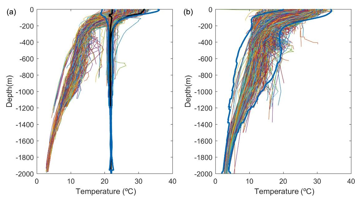
Figure 2CORA profiles inside the Red Sea (a) and in the outer region (b). The 1st and 99th quantiles of the KAUST profiles are shown in black. The range defined by 3 times the SD of the CORA profiles is shown in blue.
First, we have reviewed all the profiles to remove spikes and density inversions. In a second step, we have checked the consistency between the CORA profiles and the profiles collected by KAUST, which are considered to be more reliable as they have been thoroughly analysed by the KAUST data centre with specific criteria adapted to the region. That assessment has been performed by separating the Red Sea profiles (Fig. 2a) from the profiles obtained south of the Bab-al-Mandeb strait (labelled “Outer zone”, see Fig. 1 right). In the Red Sea, we also compute the 1 % and 99 % quantiles of the KAUST dataset (black lines in Fig. 2a), to identify potential outliers in the CORA dataset. It can be seen that two different regimes appear inside the Red Sea and are clearly identifiable by the temperatures below 500 m. Those profiles, located in the Red Sea with temperatures colder than 20 ∘C below 500 m, show a behaviour which is typical of the outside region, while such pronounced cooling with depth is absent from the KAUST profiles. Thus, those profiles are probably misplaced and have been rejected. Finally, for the rest of the profiles, those lying outside a range defined by 3 times the standard deviation (blue lines in Fig. 2) are also rejected.
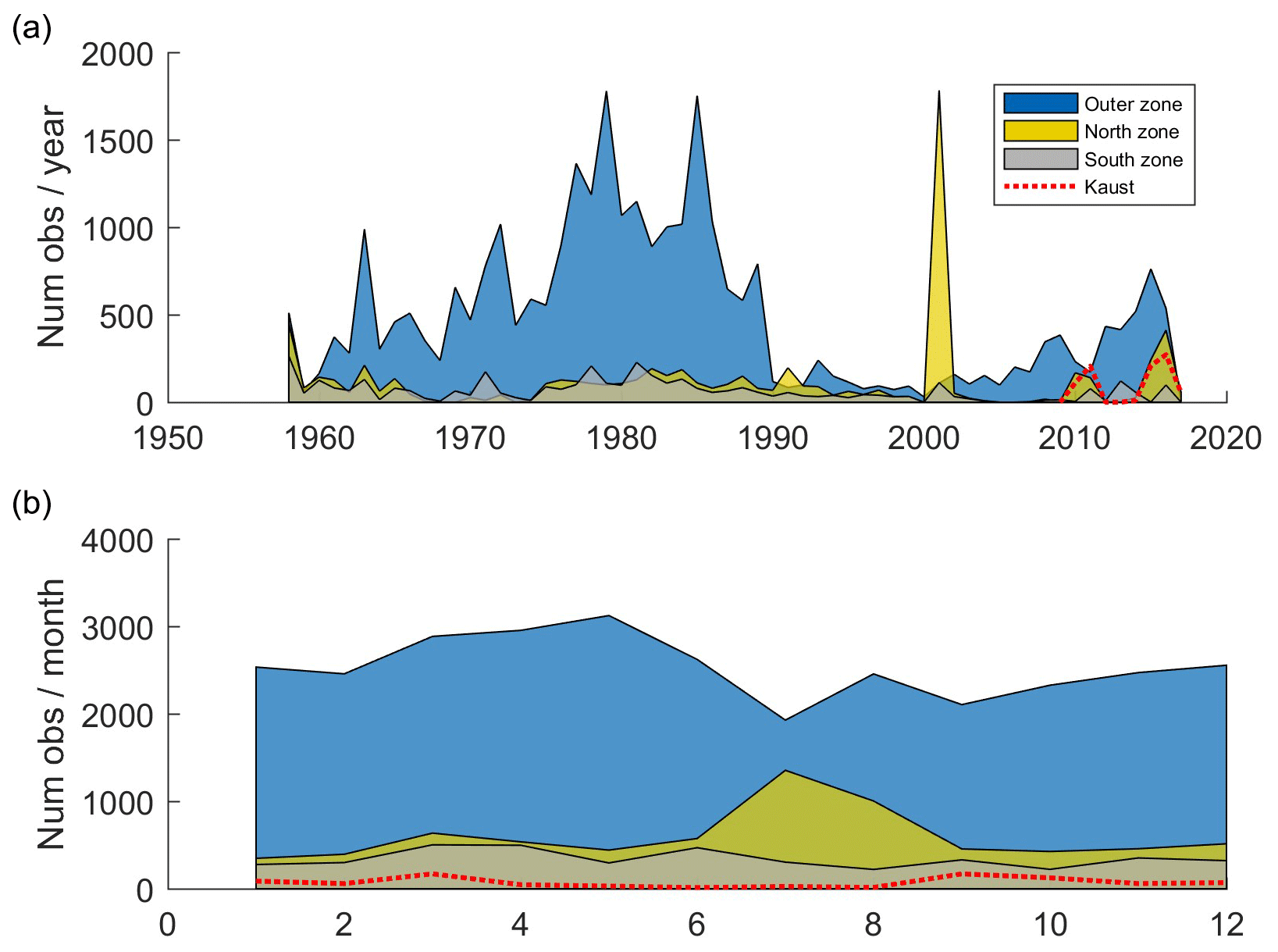
Figure 3Number of observations per year (a). Number of observations per month (b). North zone in yellow, South zone in grey and Outer zone in blue. Dashed line (in red) indicates the number of observations coming from the KAUST dataset.
After applying the quality control, 10 753 profiles are kept inside the Red Sea (82 % of initial profiles) and 29 906 are kept in the Outer zone (88 % of initial profiles). The number of observations per year and per zone is shown in Fig. 3. For the Outer zone, there is a large number of observations reaching more than 1500 profiles in some years, except during the period 1990–2000 in which the number of observations decreased. Regarding the Red Sea, the number of profiles per year in both zones is usually around 200, although in some periods there is a noticeable lack of data (e.g. during the 70s and between 2004 and 2010). In 2001, in North zone, there is a peak of observations due to an intensive campaign carried out during the summer of that year.
Considering the number of observations per month (Figs. 3, S1), we can see that it remained almost constant through the year in South zone. In contrast, the northern region is more densely sampled in summer, reaching up to more than 1000 observations in July, with roughly 500 observations on average per month during the rest of the year. Regarding the Outer zone, the number of observations per month is between 2000 and 3000, with more samples obtained during the first half of the year.
2.5 Mapping algorithm
In situ observations provide a basis for many oceanographic and meteorological applications. However, the number of observations is limited in space and time and statistical methods must be often applied to homogenize the dataset to be fitted for climate studies and/or model validation (Larsen et al., 2007). We used a classical optimal interpolation algorithm (henceforward OI; Gandin, 1966) to generate 3-D gridded monthly temperature maps from individual in situ profiles (henceforward called TEMPERSEA product).
OI is an algorithm that estimates the optimal value of the field as a linear combination of available observations and a background (i.e. first guess) field, with weights determined from the covariances of observational and background errors. The weights are obtained by minimizing the variance of the analysis error (e.g. Jordà and Gomis, 2010). Assuming we have N observations to be mapped into M grid points, the analysed field can be written in matrix form as
where BK is an M vector with the background field, S is an N×M matrix containing the covariances of the field between the observation and grid locations, D is an N×N matrix containing the covariances between observations, and d is the N vector of observed anomalies with respect to the background field:
The observations are not perfect and, assuming that observational errors are not correlated with the true field, the covariance matrix D can be split into the sum of two matrices;
where the elements of B describe the covariance of the true field between pairs of observation points , and R contains the observational error covariances . In our case we assume observational errors are decorrelated, so R becomes a diagonal matrix with observational error variances in the diagonal. To sum up, the value of the analysis field at point R is given by
For convenience, covariance matrices can be transformed to correlation matrices dividing by the field variance . This implies that the diagonal elements in R are now defined as , the noise-to-signal ratio. The correlations of the field between different locations and times are modelled using a Gaussian function for the spatial component and an exponential for the temporal component:
where dij is the distance between points i and j, and tij is the time lag. L is the spatial correlation length scale, and T is the time correlation scale.
The parameters, L, T and γ, were determined from sensitivity experiments using synthetic data. In particular, GLORYS fields are considered the “truth”. Temperature profiles are extracted from GLORYS outputs at the same time and locations that the actual profiles were obtained from. Then, the mapping algorithm is applied to those synthetic profiles and the outputs from the analysis are compared to the original GLORYS fields. Thus, we can estimate the optimal value for L and γ parameters that minimizes the error of the mapping algorithm when provided the characteristics of the observational network and the field variability. The parameter T has been estimated by computing the autocorrelation timescale from the GLORYS fields. The analysis is performed over a grid with a spatial resolution of 0.25∘ × 0.25∘ and 23 vertical depth levels unevenly distributed (Fig. 4).
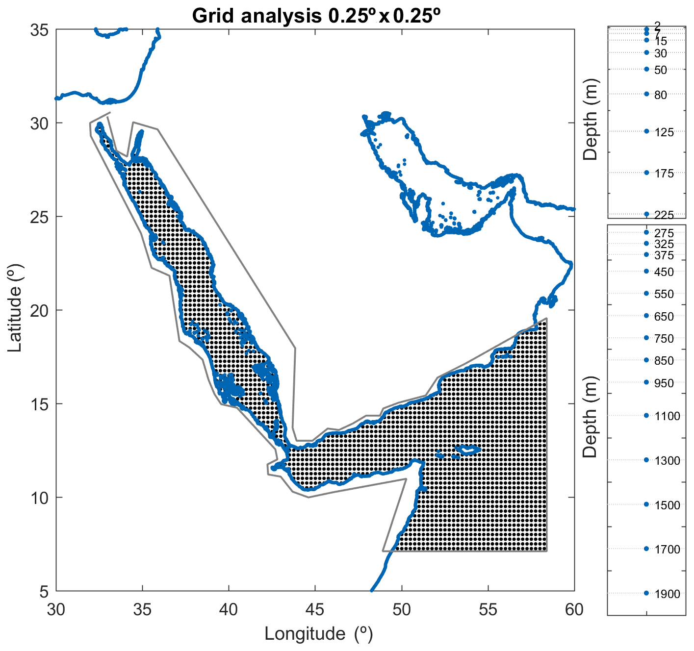
Figure 4(a) Analysis grid used in the generation of the TEMPERSEA product. (b) Depth levels.
The background (BK) used in TEMPERSEA is a 12-month climatology. This climatology is computed by merging all available observations for each month and then applying the OI algorithm to them. However, the number of profiles is often large and the inversion of the D matrix in Eq. (1) can be ill-conditioned when profiles are too close (i.e. at a distance much lower than the correlation length scale). Thus, before the OI algorithm is applied, a data thinning is performed using a K-means algorithm. This clustering technique divides the whole set of observations into a predefined number of clusters (Camus et al., 2011). In this case, each cluster represents the mean value of all the observations close to a centroid location. An example is presented in Fig. 5 for the month of January. Once we have defined the reduced set of observations grouped per month, the OI algorithm, Eq. (1), is applied using Lback=150 km and . No time correlation is considered for the computation of the climatology. Those parameters were obtained from sensitivity experiments as explained before, which also have shown that the data thinning does not degrade the quality of the background field.

Figure 5(a) Distribution of all the available observations for January (n=2705). (b) Distribution of observations after applying the K-means algorithm (n=135).
Once the climatology is computed, the analysis is performed on the anomalies with respect to it. Thus, the total temperature is computed as the combination of the background and the analysed anomaly field (see Eq. 4). For months or locations lacking observations, the analysis will tend to deliver background fields (i.e. second term in the right-hand side of Eq. 4 is zero). The parameters used for the analysis are L=200 km, T=2 months and . An example of the results of the analysed temperature anomalies for two consecutive months is shown in Fig. 6.
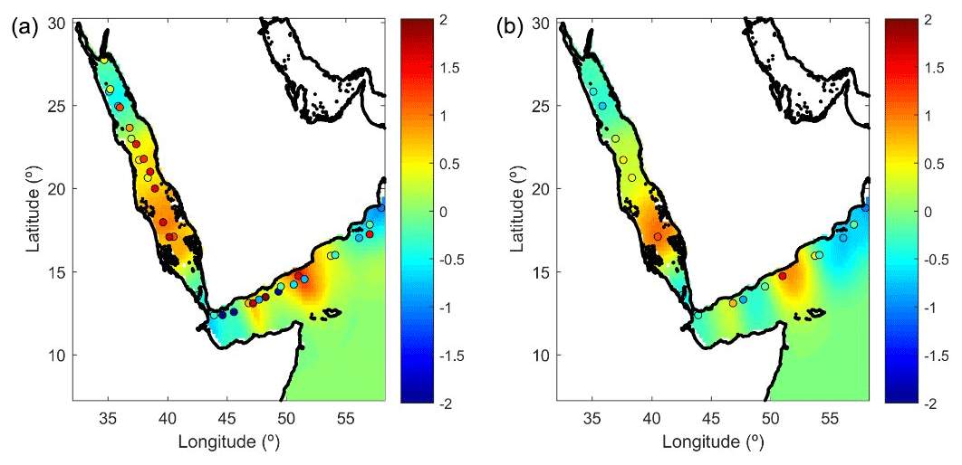
Figure 6Analysed temperature anomaly field for October 1958 (a) and November 1958 (b). The dots represent the location and value of the observations used in the analysis of each month.
2.6 Product error
One of the advantages of the OI formulation is that it also provides an estimate of the error covariances (or correlations) associated with the analysis. The M×M analysis error covariance matrix is given by
where the entries of the M×M matrix G are the correlations of the background error between pairs of analysis points, S; B and R have been defined above; and is the variance of the field. The latter is estimated from the outputs of the GLORYS model. We are particularly interested in the diagonal terms of , which give the analysis error variance ( at each of the M analysis points.
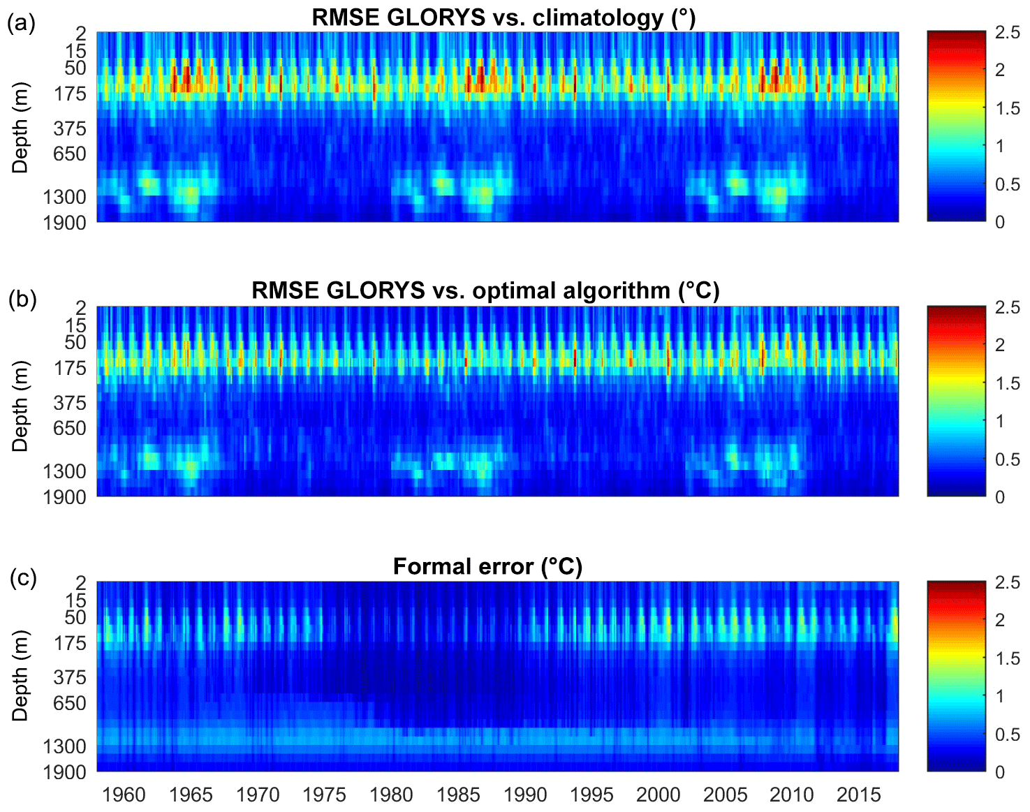
Figure 7(a) Standard deviation () of the background errors (in ∘C). (b) Root-mean-square error (RMSE, in ∘C) of the analysis fields obtained using synthetic data from GLORYS. (c) Formal error ( , in ∘C). Note the vertical axis is distorted to enhance the visualization of the upper layer.
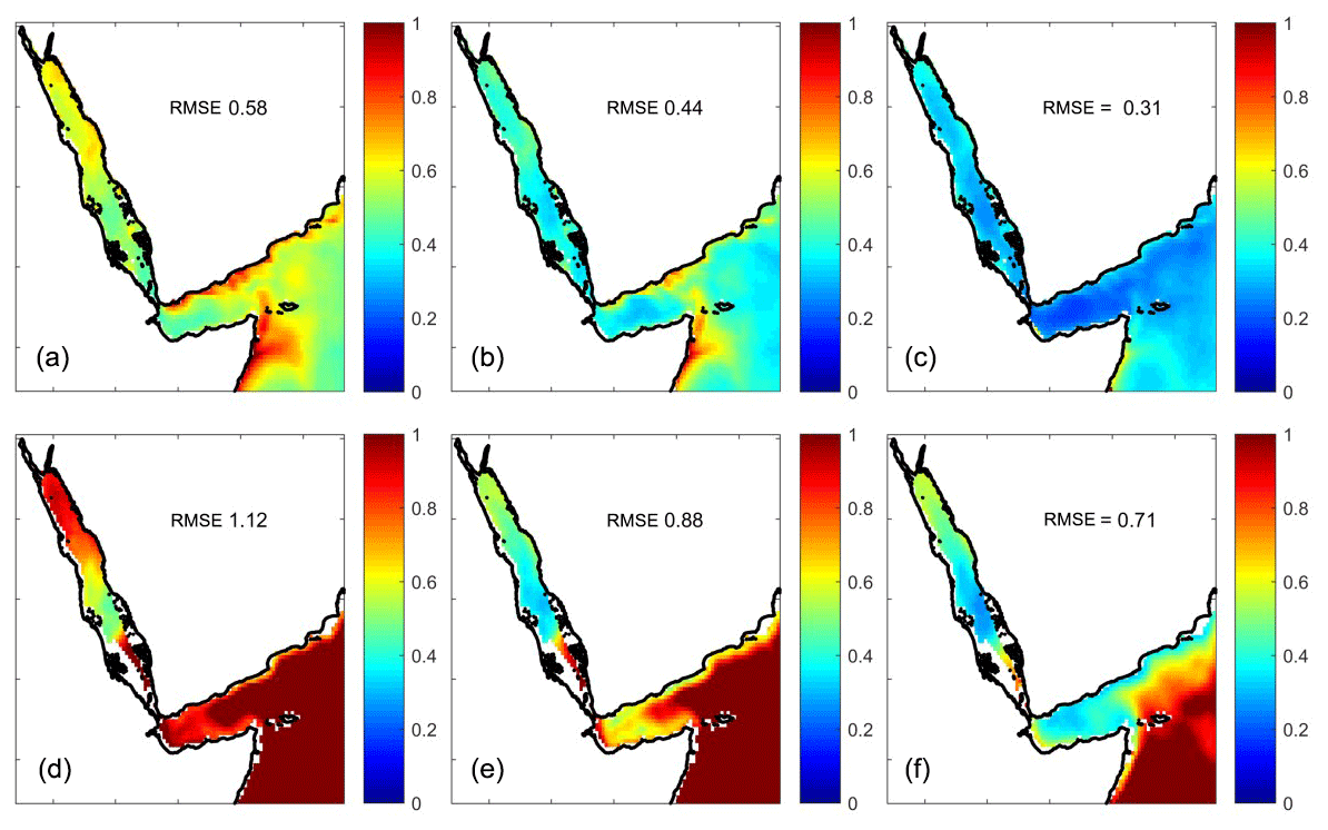
Figure 8Horizontal distribution of the RMSE (in ∘C) of the background (a, d), OI (b, e) and formal error (c, f). The results are shown for 7 m depth (a–c) and 125 m depth (d–f).
The formal estimate of the analysis error variance given by Eq. (6) depends on the number and distribution of observations as well as on the parameters chosen but not on the observations themselves. Therefore, it is useful to have a first-order estimate of the accuracy of the formal error estimates. To do so we perform a test using synthetic data from GLORYS outputs. That is, we extract pseudo-observations from GLORYS temperature fields, apply the mapping algorithm as defined above and compare the outputs with the original model fields to obtain the “true” errors. Figure 7a shows the time evolution of the RMS difference between the GLORYS outputs and the background ( averaged per vertical level, where the standard deviation (SD) of the errors in the background field was used as an estimate of the error in the temperature field. This is an important quantity as it defines the baseline error that our product has in places and times when no observations are available. Error estimates are largest at 125 m depth, with a clear seasonality in the upper layers. Below 300 m the background errors decrease well below 1 ∘C, except in some periods at 1000 m in which GLORYS data show strong, deep anomalies. Concerning the spatial distribution of the background errors (Fig. 8a), values average 0.57 ∘C at 7 m, with higher values along the Arabian coasts and in the Gulf of Aden, where background errors reach 1 ∘C. At 125 m the averaged background error is 1.12 ∘C, with minimum values in the central Red Sea (0.5 ∘C) and maximum values in the Gulf of Aden (∼1.5 ∘C), where interannual variability is more important and the climatological background is less representative of the temperature field. Figure 7b shows the time evolution of the RMSE of the analysed temperature field. Although the main features seen in the background errors are present, it is clear that using OI improves the estimate of the temperature field compared with the use of climatology, with a reduction rate ranging from 1.3 to 1.6 (i.e. errors reduced between 30 % and 60 %). The RMS error maps at 7 m show the averaged value to be reduced to 0.44 ∘C, and in most areas the reduction rate is larger than 1.5. At 125 m the RMS error is larger again in the Gulf of Aden, but the reduction rate ranges between 1.2 and 1.5. Finally, the formal error estimates are slightly lower (about 20 % lower) than the true error (Figs. 7c and 8b). However, it is able to capture the seasonality, the maximum at 125 m and the higher values around 1200 m. The error decreased between 1975 and 1990, due to the higher number of observations distributed in space and time during that period (Fig. 7), as also reflected in the true error. The formal error replicates the same spatial structure as the true error does, both at the surface layer and at 125 m. The magnitude of the formal error is slightly lower than the true error (basin averages are 0.31 and 0.44 ∘C, respectively, at the surface and 0.71 and 0.88 ∘C at 125 m).
Computing the formal error using Eq. (6) allows us to derive the formal estimate of the errors when computing regional averages. The formal estimate of the regional average can be computed as
where represents the error of the average, M is the length of analysis points and is the sum of the error covariances between all the pairs of points included in the averaging. Figure 9 shows the time evolution of the formal estimate of the average temperature in the North zone (in grey) with the true error obtained from synthetic observations (in blue). Obviously, the formal error cannot capture the actual error at each month (i.e. it is a statistical approximation), but it can be seen that it fits the SD of the true errors. Also, it is able to identify the periods in which the errors decrease (between 1975 and 2000) due to the larger density of observations. Therefore, the formal estimate seems to be a reasonable estimate of the analysis error.
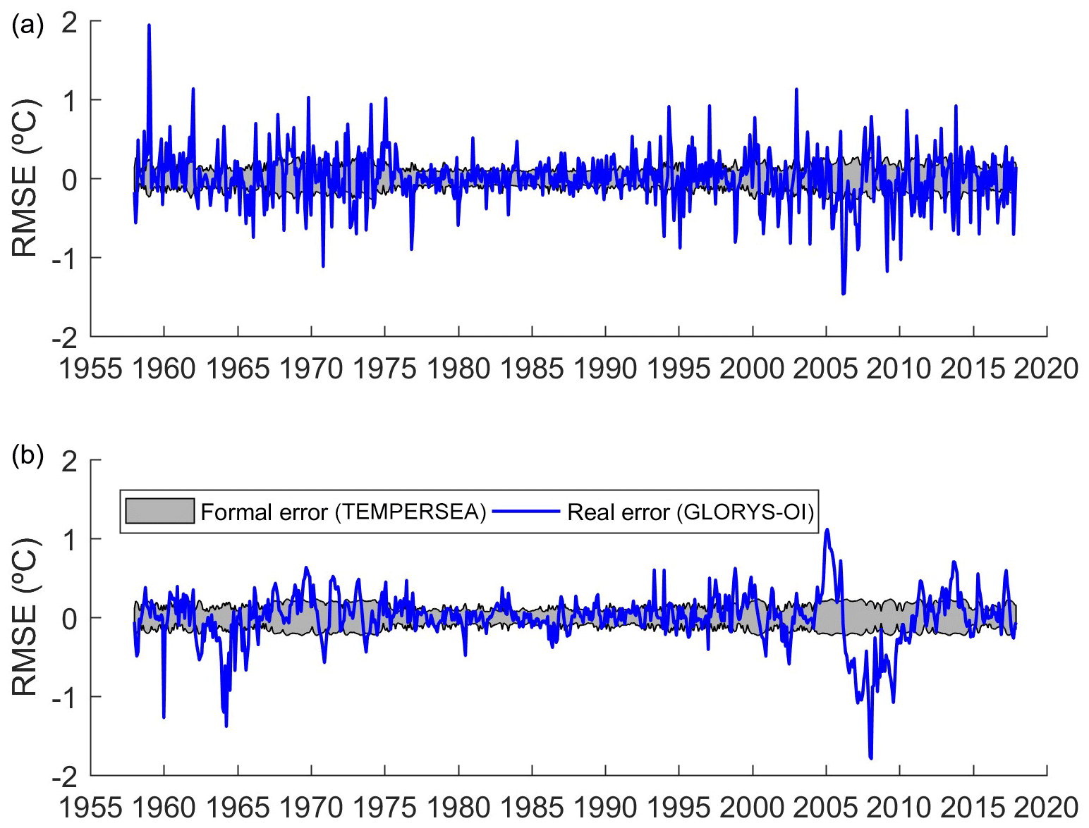
Figure 9Comparison of the formal error of the temperature average in the North zone with the true error when the algorithm is applied to synthetic data. Results shown for (a) 7 m depth and (b) 125 m depth.
3.1 Comparison with satellite results
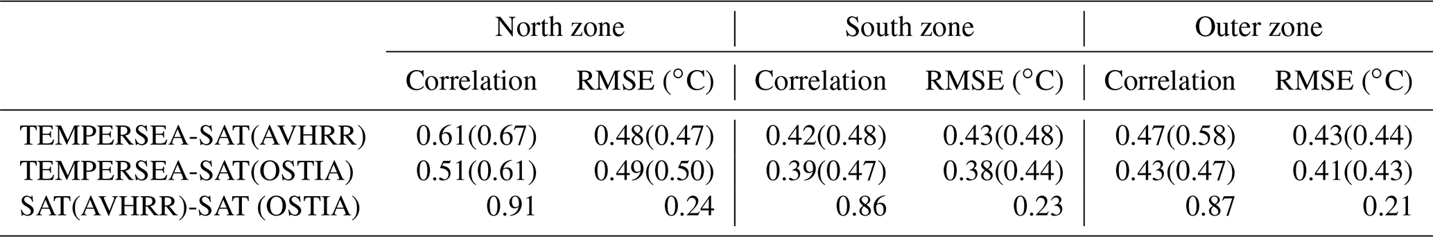
We compared the first level fields with satellite data from AVHRR and OSTIA as an independent evaluation of the TEMPERSEA product. The monthly variability of regionally averaged temperature anomalies from TEMPERSEA shows good agreement with the satellite estimates (Fig. 10). Monthly variations of ∼1 ∘C are captured by all the products as well as variations at lower frequencies. During the periods with few observations the analysis anomalies tend to zero, so the discrepancies with the satellite products increase. The correlation with AVHRR ranges between 0.42 and 0.61 and between 0.39 and 0.51 with OSTIA (Table 1). Discarding the periods with few in situ observations (i.e. with formal error > 0.15 ∘C) the monthly correlations reach 0.67 and 0.61, respectively. Regarding the RMSE the values range between 0.43 and 0.48 ∘C for AVHRR and 0.38 and 0.49 ∘C for OSTIA. It must be noted that the SST value of TEMPERSEA corresponds to the first level of the product, 2 m. This level represents the mean value of the profile temperature from the surface to 4 m of depth. In contrast, the satellite products take the value of the temperature on the first millimetres of the water column, and consequently the variability of the satellite data is larger than TEMPERSEA. Finally, both satellite estimates, although highly correlated (0.86–0.91) show important discrepancies, with RMS differences of 0.21–0.24 ∘C (Fig. 10, Table 1).
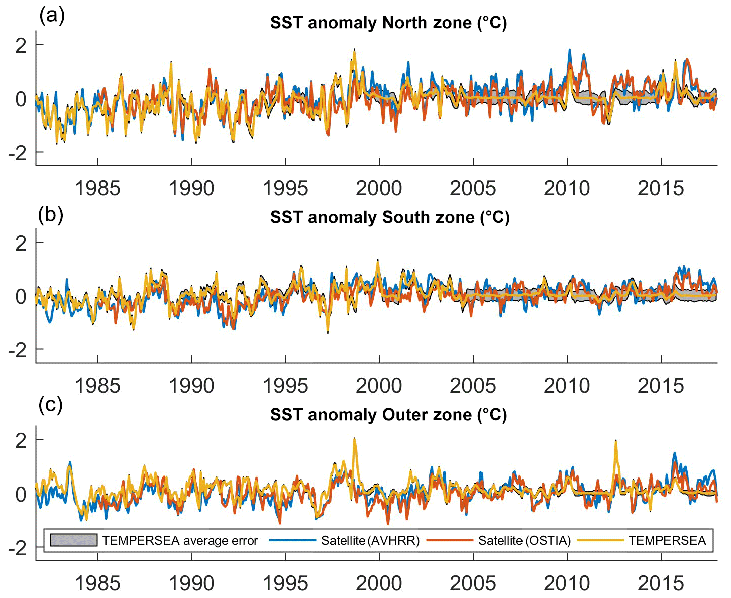
Figure 10Monthly anomalies of regionally averaged SST in the three zones, North zone (a), South zone (b) and Outer zone (c). The three datasets are shown for the common period: TEMPERSEA (yellow line), AVHRR (blue line) and OSTIA (red line). The grey patch represents the uncertainties estimated for the TEMPERSEA product.
Table 1Statistics of the comparison of regionally averaged SST monthly anomalies between TEMPERSEA, AVHRR and OSTIA. In brackets are the values when only periods with enough in situ observations (i.e. formal error < 0.15 ∘C) are considered.
3.2 Monthly climatology
We used TEMPERSEA to characterize the thermal regime of the Red Sea. The averaged field at the surface is characterized by temperatures ranging from 25.5 ∘C in the northern part of the Red Sea to 29 ∘C in the southern part, with a strong gradient at around 20∘ N (Fig. 11a). In the outer region SSTs are lower ranging from 26.5 ∘C in the Indian Ocean to 28 ∘C in the Gulf of Aden. Temperatures > 23.5 ∘C are found until a depth of 125 m inside the Red Sea, while only above 50 m in the Gulf of Aden (Fig. 11b, c). Below those depths there is a contrasting difference between the two regions, with temperatures in the Red Sea being relatively stable (∼22–24 ∘C) through the water column, while temperature decrease almost linearly with depth in the Gulf of Aden, reaching 5 ∘C at 1500 m depth, due to the oceanic influence (Sofianos and Jhons, 2015).
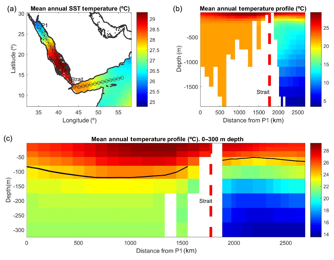
Figure 11Average temperature from TEMPERSEA computed for the period 1958–2017. (a) Averaged SST; dots indicate the location of the vertical section shown in the following figures. (b) Vertical section; (c) zoomed-in view of the vertical section for the upper 300 m. The black line indicates the isotherm of 23.5 ∘C.
The seasonal thermal evolution in the Red Sea, characterized as the anomaly of the monthly climatology relative to the annual mean, is characterized by negative anomalies in surface temperatures relative to the annual mean reaching −4 ∘C in February across the whole basin (Fig. 12). Maximum positive anomalies are found in July–August, reaching ∼4 ∘C in the northern part and –3 ∘C in the southern part. This implies that the amplitude of the seasonal cycle is larger in the northern than in the southern Red Sea. Minimum negative anomalies with respect to the annual mean in the outer region were found in August ( ∘C) and maximum anomalies ( ∘C) are found in May, with both these anomalies being larger in the open ocean than in the Gulf of Aden. These results suggest that the relative minimum found in the Gulf of Aden during summer could be induced by the advection of cold waters from the Indian Ocean.

Figure 12Monthly climatology of the surface temperatures (in ∘C).
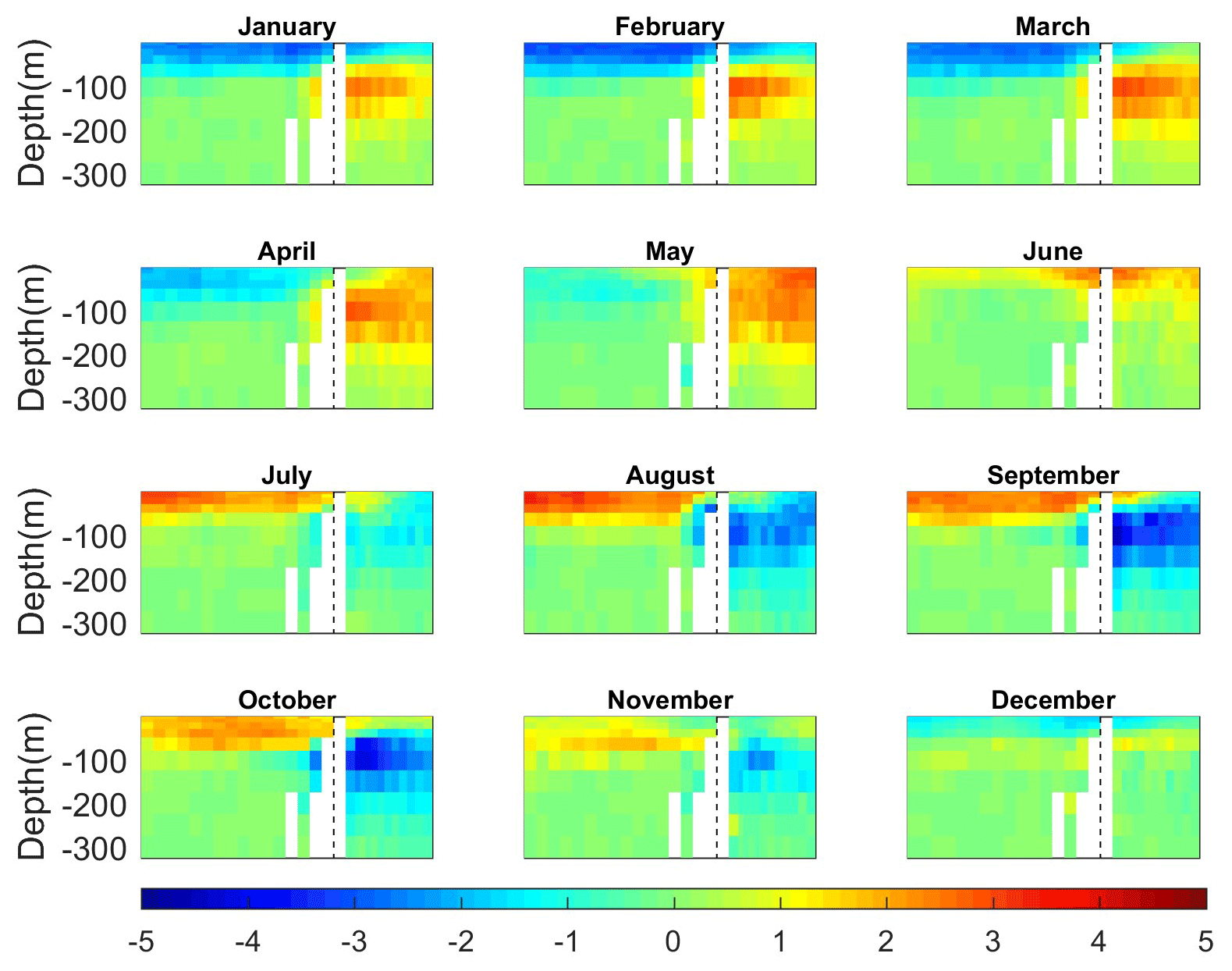
Figure 13Monthly climatology of temperature anomalies along the section depicted in Fig. 11a, with a zoomed-in view in the 0–300 m layer.
A seasonal thermal regime is only detected above 80–100 m in the Red Sea, being larger in the shallowest layers. In the Red Sea (Gulf of Aden) the larger negative anomalies are found in February (August) and the larger positive anomalies are found in August (May). The Gulf of Aden presents large seasonal variations between 50 and 200 m, with departures from the annual mean range from −4 to +4 ∘C from August and September to April and May.
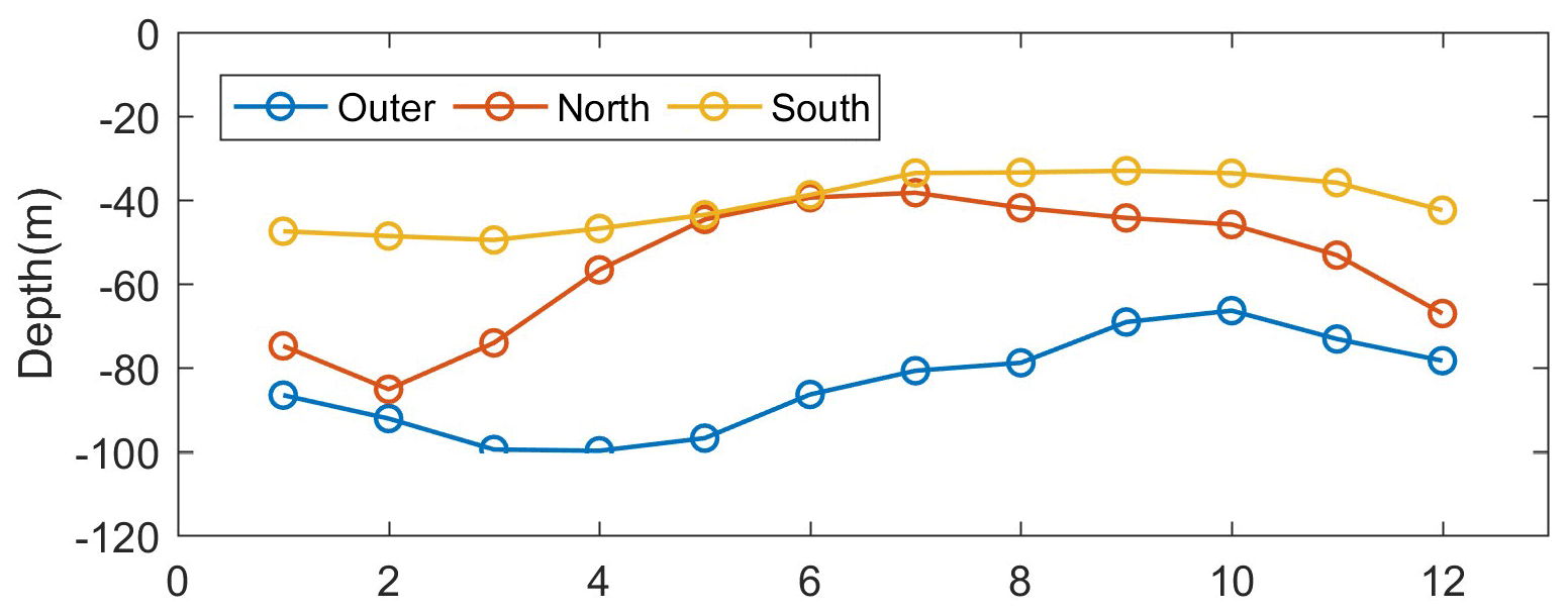
The seasonal evolution of the depth of the thermocline, defined here as the depth showing the maximum vertical temperature gradient, was computed for each grid point and then averaged regionally (Fig. 14). In the Red Sea the thermocline was deeper in February and shallower in the summer months, as expected. However, a clear difference is found between the northern and southern regions. In the northern part the thermocline is deeper, reaching 80 m in February, while in the southern part it is rather constant with monthly averaged values ranging from 35 to 50 m. In the outer region, the thermocline is deeper with maximum values of 100 m in March–May and minimum values of 70 m in September–October.
3.3 Interannual variability
In the Red Sea, the standard deviation of interannual variations of the basin averaged temperature at the sea surface and the upper layer (0–100 m) are 0.33 and 0.34 ∘C, respectively (Fig. 15), an order of magnitude lower than the seasonal changes. At the intermediate and bottom layers interannual changes are smaller (0.08 and 0.04 ∘C, respectively), but in those layers the seasonal variations are negligible, so the relative importance of low-frequency changes is larger. In the outer region, interannual changes are larger in all layers (Fig. 16) with a yearly SD of 0.38 and 0.45 ∘C in the sea surface and the upper layer (0–100 m), respectively. In the intermediate layer the interannual SD is 0.21 ∘C, more than twice larger than in the Red Sea, probably associated with lateral advection of water masses from the Indian Ocean. In the bottom layer, the yearly SD is lower, 0.05 ∘C, but still larger than in the Red Sea.
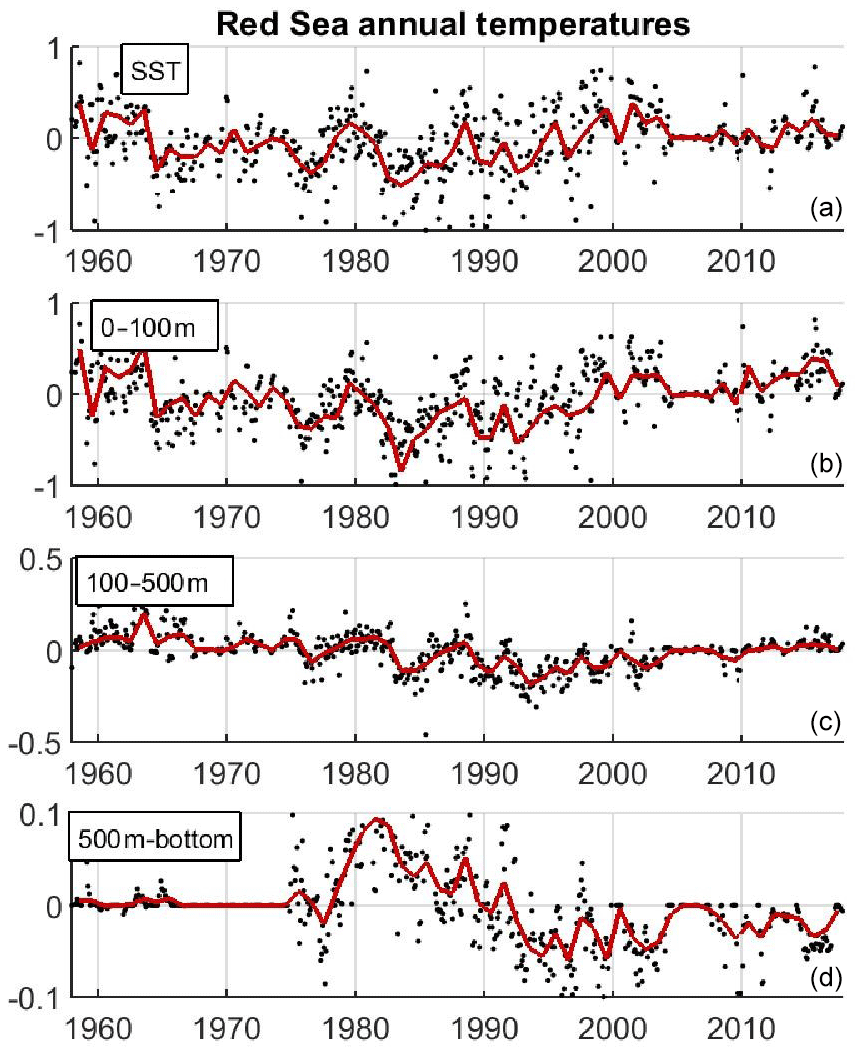
Figure 15Time series of yearly averaged temperature (in ∘C) in different layers (a) SST, (b) 0–100 m, (c) 100–500 m and (d) 500 m bottom, in the Red Sea. Black dots indicate the monthly values with formal error below 0.2 ∘C. Note the different vertical axis in each panel.
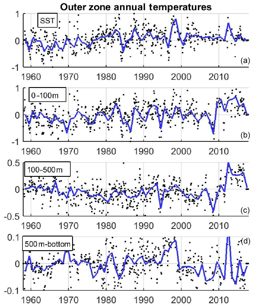
Figure 16Time series of yearly averaged temperature (in ∘C) in different layers (a) SST, (b) 0–100 m, (c) 100–500 m and (d) 500 m bottom, in the outer region. Black dots indicate the monthly values with formal error below 0.2 ∘C. Note the different vertical axis in each panel.
To characterize if the interannual variability of the temperature field is the same through the year, we have computed the standard deviation of the time series per month (i.e. 60 values per month; Fig. 17). In the Red Sea, the interannual variations are relatively small, with a SD ranging from 0.20 ∘C in January to 0.70 ∘C in November, being quite homogeneous along the basin. In the Gulf of Aden, the interannual variations are larger, particularly from May to November, when SD exceeds 1 ∘C. In the rest of the year the SD values of the interannual variations are smaller (< 0.5 ∘C).
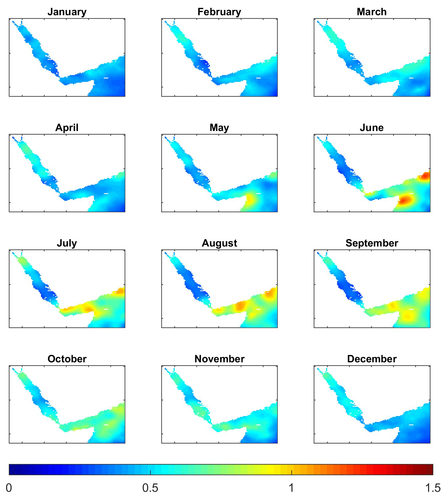
Figure 17SD of the interannual variations of surface temperature per month (in ∘C).
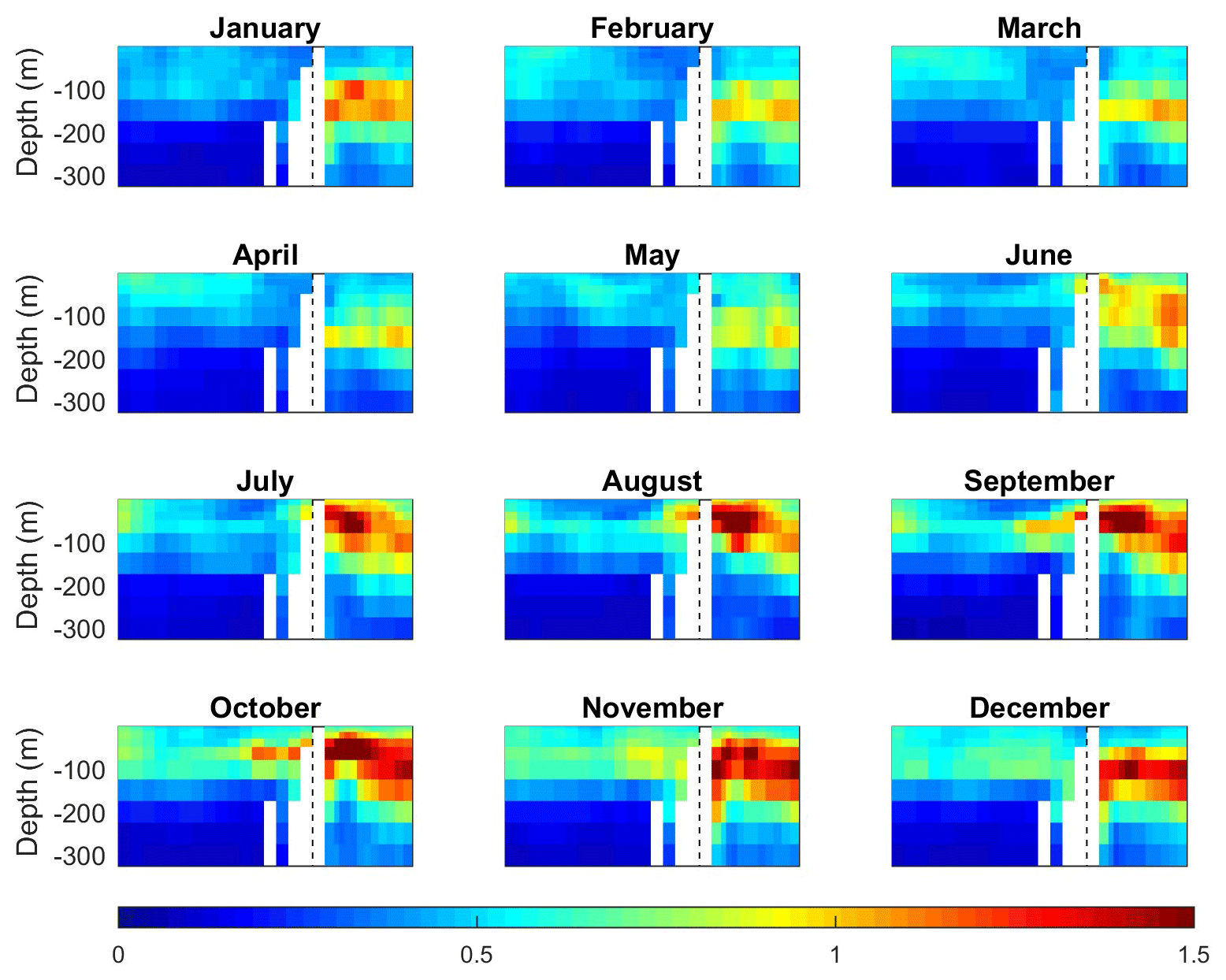
Figure 18Vertical section along the Red Sea and Gulf of Aden of the SD of interannual variations per month (in ∘C).
In the water column, the largest interannual variations are found in the Gulf of Aden, at the same location where the monthly anomalies were the largest, between 50 and 150 m (Fig. 18). The SD there even exceeds the values in the surface layer, ranging from 1 ∘C in February to up to 2 ∘C in September. Inside the Red Sea, the interannual variability decreases with depth, with a SD < 0.1 ∘C below 200 m (Fig. 18).
3.4 Multidecadal changes
The assessment of the long-term changes of the temperature field is of paramount relevance as they can shape the characteristics of the local ecosystems and may help characterize the impacts of global warming in the region. Careful examination of the interannual time series suggests that multidecadal changes are over imposed on the interannual variability. To highlight this, we extract the multidecadal variability applying a moving average with a 10-year window to the monthly time series (Fig. 19). In the Red Sea, the low-frequency component of the temperature time series in the upper layer shows a monotonous decrease from the 1960s, reaching a minimum in mid-1980s increasing monotonically since then. In the late 1960s, the temperatures were similar to those in the present decade, both being ∼0.4 ∘C above the minimum. A similar pattern applies to the intermediate layer, but the minimum was reached a decade later, in the mid 1990s. In this case, the difference between the maximum and the minimum was 0.2 ∘C, with present temperatures ∼0.05 ∘C below those in the 1960s. In the bottom layer the maximum was found in the early 1980s, while a minimum was found at the end of the 1990s. The shift in the multidecadal minima may reflect heat transfer between layers, but available information is insufficient to assess this possibility.

Figure 19Low-pass-filtered temperature time series (in ∘C) at different layers in the Red Sea and the Outer zone. A 10-year moving average was applied to the monthly time series. Note the different vertical axis in each panel.
In the outer region, the low-frequency component of the temperature in the upper layer shows an almost regular warming since the 1960s, with a relative minimum in the mid-2000s. In the intermediate layer a more complex behaviour is observed, with two relative minima (in early 1980s and mid 2000s), a relative maximum in the mid-1990s and a clear warming since mid 2000s. The evolution in the deeper layer is similar to the intermediate layer except that no clear warming is observed since the 2000s.
Finally, we computed the long-term trends in the Red Sea and the outer region at different depths. To do so, we considered that in some months there were few observations, and therefore analysed temperature anomalies were close to zero. So, in order to avoid biases in the trend estimates, months in which the formal error is greater than 0.15 ∘C are not considered in the computation.
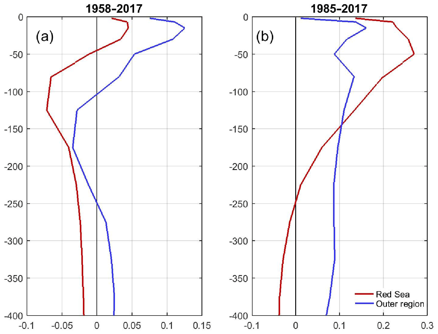
Figure 20Vertical distribution of temperature trends (in ∘C decade−1) for the Red Sea (in red) and the Outer zone (in blue). The linear trends have been computed for the periods (a) 1958–2017 and (b) 1985–2017. Note the different horizontal axis in each panel.
Trends computed for the whole TEMPERSEA time series (1958–2017; Fig. 20a) show only positive trends above 40 m depth, with maximum trends of 0.045±0.016 ∘C per decade at 15 m, and the largest negative trends at 125 m ( ∘C per decade). In the outer region trends are positive in the whole water column, except between 100 and 250 m. Maximum trends were found at 15 m (0.12±0.01 ∘C per decade) and the largest negative trends at 175 m ( ∘C per decade). For completeness, we also computed the linear trends for the satellite period (1985–2017; Fig. 20b). As the period covered by satellite observations includes the recent period of monotonous warming, trends are positive above 250 m, with maximum values found at 50 m depth (0.27±0.04 ∘C per decade). The largest negative trends are observed at 400 m ( ∘C per decade). In the outer regions, trends are positive above 800 m, with maximum values at 15 m (0.16±0.03 ∘C per decade).
The TEMPERSEA product provides a homogeneous gridded record of temperature in the whole water column based on quality-controlled in situ observations over the last 60 years. Therefore, it is a valuable complement to the more accurate, but limited on time and depth, satellite-based products. As usual in gridded products, the accuracy of TEMPERSEA is directly linked to the density of in situ profiles, which is rather heterogeneous in space and time. Therefore, use of the TEMPERSEA product should take into account the uncertainty estimates. Our comparison of the formal error estimates and direct estimates based on synthetic experiments suggest that the uncertainty estimates, both at grid point level and for the basin averages, are accurate and are a good indicator of the reliability of the product at a given time and location.
This is especially relevant when long-term trends are to be computed. The mapping procedure is a combination of the information provided by the background and by the observations. In the cases when or where no observations are available the analysis tends to the background information, which is a monthly climatology that does not change from year to year. This fact artificially damps the estimates of long-term trends (e.g. Llasses et al., 2015), so a careful treatment is needed. Our approach has been to compute trends using only those months that have enough observations (i.e. identified as those with formal error below a certain threshold). Alternatively, Good et al. (2013) use the analysis of the precedent month as the background field. This allows for the propagation of long-term changes and may produce a better estimate of the long-term trends. However, it also may induce spurious trends if sustained periods without observations exist (i.e. several years), so this approach should be carefully explored in future analyses of TEMPERSEA.
Another interesting feature of the uncertainty estimate is that it allows for identification of sampling strategies that have led in the past to high accuracies and thus that could be used to guide future monitoring efforts of Red Sea temperatures. The formal error decreases with the number of observations, but the spatial distribution of the observations also plays an important role. In TEMPERSEA more than 70 months in which the error is as low as 0.1 ∘C with less than 10 observations have been identified (Fig. 21). Conversely, in some months with intensive campaigns more than 500 profiles have been collected, but the formal error did not decrease further. The reason for this is that observations separated less than the typical correlation length scale (i.e. the spatial scale of the process dominating the temperature variability) provide redundant information. On the other hand, we have identified months in which, surprisingly, no observations were gathered in the Red Sea. As mentioned before, this represents a serious limitation to accurately quantify long-term changes. Therefore, if the goal is to characterize the climatic evolution of the Red Sea temperature, an optimized sampling should be designed to minimize the number of required profiles, with approximately less than 10 profiles needed per month. However, this should be repeated monthly, or at least seasonally, to ensure the continuity of the record and to reduce the noise in the long-term change estimates.
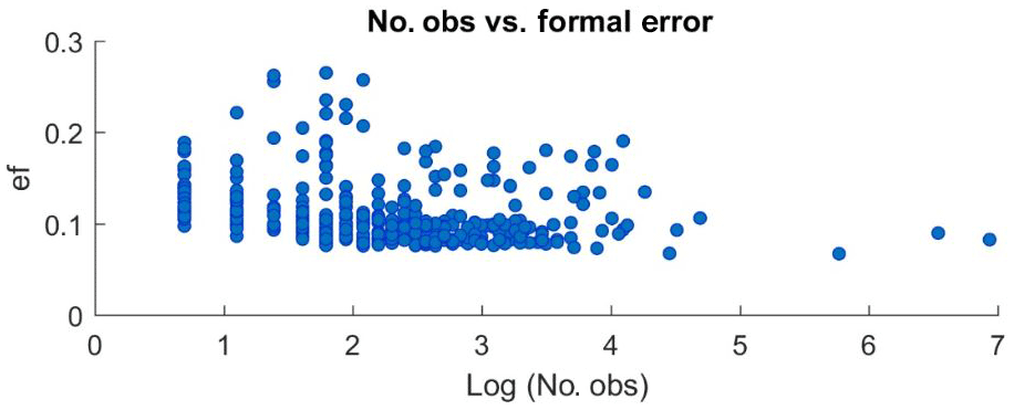
Figure 21Scatter plot of the formal error vs. log of the number of observations per month used to compute the maps.
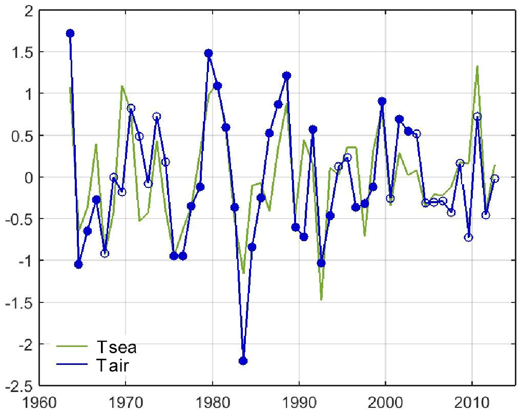
Figure 22Normalized air temperature at 1000 mbar (green) and 0–100 m sea temperature (blue) in the Red Sea. A high-pass filter has been applied to remove multidecadal variations. Solid dots indicate an averaged formal error below 0.15 ∘C.
TEMPERSEA has allowed us to characterize the 3-D variability of the temperature field in the Red Sea and the adjacent Arabian Sea, which show a different behaviour. In the Red Sea most variability is induced by surface processes with little variability at intermediate or deep layers. Conversely, in the Gulf of Aden and the Arabian Sea the influence of lateral advection plays an important role in inducing a shift in the seasonal cycle and large interannual variations in subsurface layers. In order to get a deeper insight into the role of the atmosphere in the sea temperature variations, we analysed air temperatures at 1000 mbar (representative of air in contact with sea surface) and 850 mbar (representative of air masses not directly affected by air–sea interactions, as it corresponds to roughly 1450 m of altitude). In particular we used the output from the JRA55 atmospheric reanalysis for the period 1958–2014 (Harada et al., 2015), and extend it with the output from the National Centers for Environmental Prediction (NCEP) reanalysis (Kanamitsu et al., 2002) for the period 2014–2017. Before merging both datasets we ensured homogeneity in terms of mean and variance during the common period. The air temperatures have been averaged over the Red Sea and the outer region and compared with the sea temperatures at different layers. In order to isolate the interannual variations we have removed the multidecadal variations using a 10-year moving average high-pass filter.
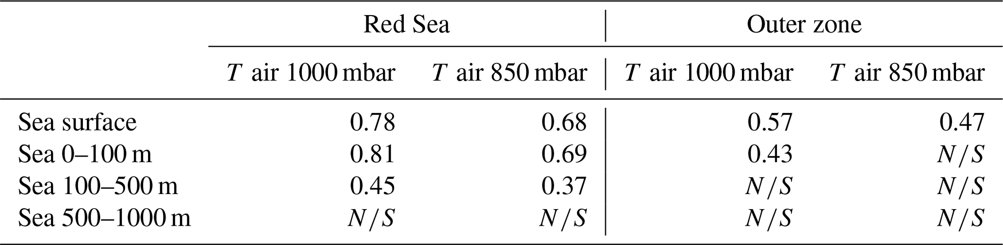
In the Red Sea the results show a very good correlation between air temperature at 1000 mbar and temperatures at the sea surface and in the 0–100 m layer (correlations of 0.78 and 0.81, respectively; see Fig. 22 and Table 2). When air temperature at 850 mbar is used, the correlations decrease but are still high (0.68 and 0.69, respectively). This means that most interannual variations in the upper layer of the Red Sea can be explained by large-scale changes in air temperature. A non-negligible part (∼15 % of the variance) can be attributed to air–sea interactions. The effects of atmosphere variability are also detected in the intermediate layer, where the correlation is 0.45. No statistically significant correlations were found in the deeper layers. Concerning the Gulf of Aden, the correlation between air and sea temperatures is lower and restricted to the upper layer (see Table 2). This reinforces the hypothesis that lateral advection plays an important role in driving the interannual variations of temperature in the Gulf of Aden and the Arabian Sea.
Table 2Correlation between air and sea temperatures in the Red Sea and the Outer zone. Two heights are used for the air, 1000 mbar, representative of the lower layers of the atmosphere in contact with the sea, and 850 mbar, representative of the temperature in altitude (roughly 1450 m height). Only years with averaged formal error below 0.15 ∘C are considered. All values are significant at the 95 % level (N∕S indicated otherwise).
Finally, multidecadal changes have been assessed with the TEMPERSEA product, showing a non-negligible contribution to temperature variability. This is an important result for the interpretation of long-term trends. Linear trends are often computed as an indicator of potential influence of global warming. However, the trends can be masked by low-frequency variations when their period is comparable to the length of the record (Jordà, 2014). This is clear for the temperature records in the Red Sea derived from the TEMPERSEA product. For instance, our results suggest that sea temperature in the upper layer, in the 1960s, was similar to the present values, so a very small, positive trend is obtained when the period 1958–2017 is used, consistent with recent evidence of long-term thermal oscillations in the Red Sea (Krokos et al., 2019). For the intermediate layer, the sign of the trend is even reversed, as the temperatures in the 1960s were higher than those recorded in recent years. Conversely, if only the last 30 years are considered, which is also the period covered by the satellite record, trends are strong and positive, and therefore easily misinterpreted as linked to global warming. Hence, the conclusions, based on satellite records, that the Red Sea is warming at rates faster than the global ocean (Chaidez et al., 2017; Raitsos et al., 2011), based on the satellite record, need to be reconsidered, as warming rates retrieved for 1958–2017 with the TEMPERSEA product are 10-fold lower than those retrieved from satellite records covering the past 30 years.
An observation-based high-resolution homogeneous 3-D temperature product has been developed for the Red Sea for the period 1958–2017 (the TEMPERSEA product). For that, two databases of in situ observations (CORA and KAUST) were merged and quality controlled, resulting in a dataset of 40 659 profiles (10 753 in the Red Sea and 29 906 in the Gulf of Aden). A mapping procedure based on optimal interpolation was applied to those profiles to compute two gridded products: a 12-month climatology and a 60-year monthly product. In order to calibrate the algorithm, synthetic data from a realistic numerical model have been used. Furthermore, the formal error from optimal interpolation has been computed and has proven to be a good approximation to actual uncertainty. The TEMPERSEA product is available from the open data repository PANGAEA (Agulles et al., 2019).
The product has been compared to satellite observations for the period 1981–2017, showing reasonable agreement in terms of spatial and temporal variability at monthly, seasonal and interannual scales. Also, very good agreement has been found between air temperatures from the atmospheric reanalyses and reconstructed sea temperatures for the whole period 1958–2017, enhancing confidence in the quality of the product.
The TEMPERSEA product allowed us to characterize the climatology of the temperature in the region. In the Red Sea, the maximum temperatures are found south of 20∘ N, while the minimum is found in the northern part. Regarding the seasonal cycle, it peaks in August and is minimum in February. The seasonal cycle is larger in the northern part, while in the southern part it is smaller in terms of the thermal range in surface waters. In the Gulf of Aden, the phase and shape of the seasonal cycle is different with maximum values in May and minimum values in August. Related to the vertical structure of the temperature field, our results show a large difference between the Red Sea and the Gulf of Aden, especially below the depth of the Bab-al-Mandeb strait. The strait isolates the Red Sea allowing it to have temperatures above 20 ∘C in the whole water column, while the Gulf of Aden, influenced by the open ocean variability shows a vertical structure typical of the Indian Ocean, with temperatures reaching 5 ∘C at 1000 m depth. Furthermore, the length of the product has allowed us to characterize multidecadal variability at different layers. Our results show that multidecadal variations have been important in the past and can bias the trends computed from 30 to 40 years of data.
TEMPERSEA provides a reference product to describe the temporal evolution of the 3-D temperature field in the Red Sea and to calibrate and validate numerical models. This will allow us to improve forecasting models and formulate more reliable predictions and climate projections. It has also been shown that the quality of the product is critically linked to the existence of in situ observations. Periods with few observations degrade the quality of the product, so it is important to keep a regular monitoring of the region in order to identify new changes and to remove uncertainties in the climate studies. TEMPERSEA provides a basis to design an optimal sampling programme to track the thermal dynamics of the Red Sea. Our results suggest that an effective monitoring can be achieved with few, strategically located, observations.
The TEMPERSEA product is freely available at PANGAEA repository (https://www.pangaea.de/).
The supplement related to this article is available online at: https://doi.org/10.5194/os-16-149-2020-supplement.
MA and GJ wrote the main article text; BJ provided the Kaust data; all co-authors reviewed the article and figures.
The authors declare that they have no conflict of interest.
This research was funded by King Abdullah University of Science and Technology (KAUST) through funds provided to S.A. and C.M.D (BAS/1/1072-01-01).
Migeul Agulles has been partly funded by the European Union's Horizon 2020 research and innovation programme under grant agreement no. 776661 (SOCLIMPACT project).
This research has been supported by the King Abdullah University of Science and Technology (KAUST) (grant no. BAS/1/1072-01-01) and the European Commission (SOCLIMPACT (grant no. 776661)).
This paper was edited by Trevor McDougall and reviewed by three anonymous referees.
Bell, M. J., Forbes, R. M., and Hines, A.: Assessment of the FOAM global data assimilation system for real-time operational ocean forecasting, J. Mar. Syst., 25, 1–22, https://doi.org/10.1016/S0924-7963(00)00005-1, 2000.
Bongaerts, P., Ridgway, T., Sampayo, E. M., and Hoegh-Guldberg, O.: Assessing the “deep reef refugia” hypothesis: Focus on Caribbean reefs, Coral Reefs, 29, 1–19, https://doi.org/10.1007/s00338-009-0581-x, 2010.
Cabanes, C., Grouazel, A., von Schuckmann, K., Hamon, M., Turpin, V., Coatanoan, C., Paris, F., Guinehut, S., Boone, C., Ferry, N., de Boyer Montégut, C., Carval, T., Reverdin, G., Pouliquen, S., and Le Traon, P.-Y.: The CORA dataset: validation and diagnostics of in-situ ocean temperature and salinity measurements, Ocean Sci., 9, 1–18, https://doi.org/10.5194/os-9-1-2013, 2013.
Camus, P., Mendez, F. J., Medina, R., and Cofiño, A. S.: Analysis of clustering and selection algorithms for the study of multivariate wave climate, Coast. Eng., 58, 453–462, https://doi.org/10.1016/j.coastaleng.2011.02.003, 2011.
Chaidez, V., Dreano, D., Agusti, S., Duarte, C. M., and Hoteit, I.: Decadal trends in Red Sea maximum surface temperature, Sci. Rep., 7, 1–8, https://doi.org/10.1038/s41598-017-08146-z, 2017.
Dee, D. P., Uppala, S. M., Simmons, A. J., Berrisford, P., Poli, P., Kobayashi, S., Andrae, U., Balmaseda, M. A., Balsamo, G., Bauer, P., Bechtold, P., Beljaars, A. C. M., van de Berg, L., Bidlot, J., Bormann, N., Delsol, C., Dragani, R., Fuentes, M., Geer, A. J., Haimberger, L., Healy, S. B., Hersbach, H., Hólm, E. V., Isaksen, L., Kållberg, P., Köhler, M., Matricardi, M., Mcnally, A. P., Monge-Sanz, B. M., Morcrette, J. J., Park, B. K., Peubey, C., de Rosnay, P., Tavolato, C., Thépaut, J. N., and Vitart, F.: The ERA-Interim reanalysis: Configuration and performance of the data assimilation system, Q. J. Roy. Meteorol. Soc., 137, 553–597, https://doi.org/10.1002/qj.828, 2011.
Eladawy, A., Nadaoka, K., Negm, A., Abdel-Fattah, S., Hanafy, M., and Shaltout, M.: Characterization of the northern Red Sea's oceanic features with remote sensing data and outputs from a global circulation model, Oceanologia, 59, 213–237, https://doi.org/10.1016/j.oceano.2017.01.002, 2017.
Ferry, N., Parent, L., Garric, G., Barnier, B., and Jourdain, N.: Mercator global eddy permitting ocean reanalysis GLORYS1V1: Description and results, Mercat, Ocean Q. Newsl., 36, 15–27, 2010.
Gandin, L. S.: Objective analysis of meteorological fields. By L. S. Gandin. Translated from the Russian. Jerusalem (Israel Program for Scientific Translations), 1965. Pp. vi, 242: 53 Figures; 28 Tables. £4 1s. 0d, Q. J. Roy. Meteor. Soc., 92, 447–447, doi:10.1002/qj.49709239320, 1966.
Good, S. A., Martin, M. J., and Rayner, N. A.: EN4: Quality controlled ocean temperature and salinity profiles and monthly objective analyses with uncertainty estimates, J. Geophys. Res.-Oceans, 118, 6704–6716, https://doi.org/10.1002/2013JC009067, 2013.
Harada, Y., Ebita, A., Ota, Y., Onogi, K., Takahashi, K., Endo, H., Miyaoka, K., Kobayashi, S., Onoda, H., Moriya, M., Kamahori, H., and Kobayashi, C.: The JRA-55 Reanalysis: General Specifications and Basic Characteristics, J. Meteorol. Soc. Jpn. Ser. II, 93, 5–48, https://doi.org/10.2151/jmsj.2015-001, 2015.
Ishii, M. and Kimoto, M.: Reevaluation of historical ocean heat content variations with time-varying XBT and MBT depth bias corrections, J. Oceanogr., 65, 287–299, https://doi.org/10.1007/s10872-009-0027-7, 2009.
Jordà, G.: Detection time for global and regional sea level trends and accelerations, J. Geophys. Res.-Ocean., 119, 2121–2128, doi:10.1002/2014JC010005, 2014.
Jordà, G. and Gomis, D.: Accuracy of SMOS level 3 SSS products related to observational errors, IEEE T. Geosci. Remote Sens., 48, 1694–1701, https://doi.org/10.1109/TGRS.2009.2034259, 2010.
Kanamitsu, M., Ebisuzaki, W., Woollen, J., Yang, S.-K., Hnilo, J. J., Fiorino, M., and Potter, G. L.: NCEP-DOE AMIP-II Renalalysys (R-2), B. Am. Meteorol. Soc., 83, 1631–1643, doi:10.1175/BAMS-83-11 -1631, 2002.
Karnauskas, K. B. and Jones, B. H.: The Interannual Variability of Sea Surface Temperature in the Red Sea From 35 Years of Satellite and In Situ Observations, J. Geophys. Res.-Oceans, 123, 5824–5841, https://doi.org/10.1029/2017JC013320, 2018.
Krokos, G., Papadopoulos, V. P., Sofianos, S. S., Ombao, H., Dybczak, P., and Hoteit, I.: Natural Climate Oscillations may Counteract Red Sea Warming Over the Coming Decades, Geophys. Res. Lett., 46, 3454–3461, https://doi.org/10.1029/2018GL081397, 2019.
Larsen, J., Høyer, J. L., and She, J.: Validation of a hybrid optimal interpolation and Kalman filter scheme for sea surface temperature assimilation, J. Mar. Syst., 65, 122–133, https://doi.org/10.1016/j.jmarsys.2005.09.013, 2007.
Lima, F. P. and Wethey, D. S.: Three decades of high-resolution coastal sea surface temperatures reveal more than warming, Nat. Commun., 3, 1–13, https://doi.org/10.1038/ncomms1713, 2012.
Llasses, J., Jordà, G., and Gomis, D.: Skills of different hydrographic networks in capturing changes in the Mediterranean Sea at climate scales, Clim. Res., 63, 1–18, https://doi.org/10.3354/cr01270, 2015.
Neumann, A. C. and McGill, D. A.: Circulation of the Red Sea in early summer, Deep-Sea Res., 8, 223–235, https://doi.org/10.1016/0146-6313(61)90023-5, 1961.
Patzert, W. C.: Wind-induced reversal in Red Sea circulation, Deep. Res. Oceanogr. Abstr., 21, 109–121, https://doi.org/10.1016/0011-7471(74)90068-0, 1974.
Poloczanska, E. S., Burrows, M. T., Brown, C. J., García Molinos, J., Halpern, B. S., Hoegh-Guldberg, O., Kappel, C. V., Moore, P. J., Richardson, A. J., Schoeman, D. S., and Sydeman, W. J.: Responses of Marine Organisms to Climate Change across Oceans, Front. Mar. Sci., 3, 1–21, https://doi.org/10.3389/fmars.2016.00062, 2016.
Raitsos, D. E., Hoteit, I., Prihartato, P. K., Chronis, T., Triantafyllou, G., and Abualnaja, Y.: Abrupt warming of the Red Sea, Geophys. Res. Lett., 38, 1–5, https://doi.org/10.1029/2011GL047984, 2011.
Roberts-Jones, J., Fiedler, E. K., and Martin, M. J.: Daily, global, high-resolution SST and sea ice reanalysis for 1985-2007 using the OSTIA system, J. Climate, 25, 6215–6232, https://doi.org/10.1175/JCLI-D-11-00648.1, 2012.
Sofianos, S. and Johns, W. E.: Water Mass Formation, Overturning Circulation, and the Exchange of the Red Sea with the Adjacent Basins, Nature, 93, 163–164, doi:10.1007/978-3-662-45201-1_20, 2015.
Thorne, K. S., Wheeler, J. A., Francisco, S., Wieman, C. E., Ertmer, W., Schleich, W. P., Rasel, E. M., Diego, S., Chung, K. Y., Chu, S., Scully, M. O., Physics, A., Grynberg, G., Stora, R., Pavlis, E. C., and Wheeler, J. A.: References and Notes 1, Science, 327, 1543–1548, https://doi.org/10.1126/science.1206034, 2010.
Werner, F. and Lange, K.: A bathymetric survey of the sill area between the Red Sea and the Gulf of Aden, Geologisches Jahrbuch D, 13, 125–130, 1975.