the Creative Commons Attribution 4.0 License.
the Creative Commons Attribution 4.0 License.
 | 18 Nov 2020
Importance of El Niño reproducibility for reconstructing historical CO2 flux variations in the equatorial Pacific
Hiroaki Tatebe
Hiroshi Koyama
Tomohiro Hajima
Masahiro Watanabe
Michio Kawamiya
Based on a set of climate simulations utilizing two kinds of Earth system models (ESMs) in which observed ocean hydrographic data are assimilated using exactly the same data assimilation procedure, we have clarified that the successful simulation of the observed air–sea CO2 flux variations in the equatorial Pacific is tightly linked to the reproducibility of coupled physical air–sea processes. When an ESM with a weaker ENSO (El Niño–Southern Oscillations) amplitude than that of the observations was used for historical simulations with ocean data assimilation, the observed equatorial anticorrelated relationship between the sea surface temperature (SST) and the air–sea CO2 flux on interannual to decadal timescales could not be represented. The simulated CO2 flux anomalies were upward (downward) during El Niño (La Niña) periods in the equatorial Pacific. The reason for this was that the non-negligible correction term in the governing equation of ocean temperature, which was added via the ocean data assimilation procedure, caused an anomalous, spurious equatorial upwelling (downwelling) during El Niño (La Niña) periods, which brought more (less) subsurface layer water rich in dissolved inorganic carbon (DIC) to the surface layer. On the other hand, in the historical simulations where the observational data were assimilated into the other ESM with a more realistic ENSO representation, the correction term associated with the assimilation procedure remained small enough so as not to disturb an anomalous advection–diffusion balance for the equatorial ocean temperature. Consequently, spurious vertical transport of DIC and the resultant positively correlated SST and air–sea CO2 flux variations did not occur. Thus, the reproducibility of the tropical air–sea CO2 flux variability with data assimilation can be significantly attributed to the reproducibility of ENSO in an ESM. Our results suggest that, when using data assimilation to initialize ESMs for carbon cycle predictions, the reproducibility of the internal climate variations in the model itself is of great importance.
- Article
(6109 KB) - Full-text XML
-
Supplement
(2196 KB) - BibTeX
- EndNote


Since the industrial revolution, vast quantities of greenhouse gases (e.g., CO2) have been released into the atmosphere through human activities such as fossil fuel use and land use change. This increased atmospheric CO2 concentration leads to global warming; however, both the oceanic and the terrestrial ecosystems absorb atmospheric CO2 and are considered to work to relax the progress of the global warming (Sabine et al., 2004; Doney et al., 2009a, 2014; Le Quéré et al., 2009, 2010, 2016). Observation-based studies have reached the consensus that significant interannual variability in the air–sea CO2 flux (hereafter CO2F) exists in some specific regions, such as the equatorial Pacific and the high latitudes of both hemispheres (e.g., Park et al., 2010; Valsala and Maksyutov, 2010; Landschützer et al., 2014; Rödenbeck et al., 2014), and the variation in CO2F associated with the El Niño–Southern Oscillation (ENSO) in the equatorial Pacific has been highlighted in many previous observation-based and simulation-based studies (Keeling and Revelle, 1985; Feely et al., 1997, 1999; Jones et al., 2001; Obata and Kitamura, 2003; McKinley et al., 2004; Patra et al., 2005). When an El Niño event occurs in the equatorial Pacific, the dissolved inorganic carbon (DIC) concentration in the surface layer decreases due to a reduction in the supply of cold, DIC-rich subsurface water to the surface layer compared with normal years, which stems from weaker equatorial upwelling associated with weaker trade winds (Le Borgne et al., 2002; Feely et al., 2004; Doney et al., 2009a, b). Correspondingly, the CO2F anomaly is downward during El Niño, and the inverse is seen during La Niña. Le Borgne et al. (2002) estimated that the upwelling of DIC-rich subsurface water accounts for up to 70 % of the CO2F variation in the equatorial Pacific, while the other 30 % is attributable to variation in the wind speed and biological processes. Accordingly, to estimate and predict variations in CO2 uptake by the global ocean on timescales of several years, it would be informative to first consider the variations in the equatorial Pacific associated with ENSO.
The Paris Agreement is an agreement within the United Nations Framework Convention on Climate Change (UNFCCC, 2015) providing the framework of measures from 2021 to 2030 to act against climate change. The goal of the Paris Agreement is to restrict the rise in the global mean surface air temperature to well below 2 ∘C relative to the preindustrial level. If greenhouse gas emissions continue to increase at their current rate, the Earth's surface will warm by 1.5 ∘C within ∼ 20 years relative to the preindustrial state as reported in the Fifth Assessment Report (AR5) of the Intergovernmental Panel on Climate Change (IPCC, 2013). In this context, comprehensive understanding of the changes in the carbon cycle over previous years is essential for accurate predictions of the global carbon cycle, including natural variations, which will assist in evaluation of future CO2 emission reductions (Kawamiya et al., 2020).
For future climate predictions, data assimilation procedures are incorporated into climate models in order to synchronize simulated climatic states in the model with observations, that is, the initialization of climate models. By incorporating data assimilation procedures into Earth system models (ESMs), it will be possible to reproduce and predict variations in biogeochemical properties (Brasseur et al., 2009; Tommasi et al., 2017a, b; Park et al., 2018). This includes an assessment of the predictability of CO2F on a decadal timescale for the global ocean (Li et al., 2016, 2019).
Focusing on CO2F fluctuations associated with ENSO in the equatorial Pacific, Dong et al. (2016) analyzed the results of the Earth system models (ESMs) that participated in the Coupled Model Intercomparison Project Phase 5 (CMIP5; Taylor et al., 2012), which contributed to the AR5 of the Intergovernmental Panel on Climate Change (IPCC, 2013). They showed that only some ESMs could reproduce the observed anticorrelated relationship between SST and CO2F. This suggests that our understanding of ENSO and associated global carbon cycle variations are still insufficient. For reliable prediction of future CO2 uptake on interannual to decadal timescales, it is necessary to understand coupled physical air–sea processes and the associated carbon cycle variations in the equatorial Pacific.
In this study, utilizing two kinds of ESMs in which observed ocean hydrographic data are assimilated, we attempted to identify the key processes to reproduce the observed historical air–sea CO2 flux variations in the equatorial Pacific. The remainder of this paper is organized as follows: Sect. 2 provides a brief description of the models used in this study, the derived results are presented in Sect. 3, and a short discussion and summary are presented in Sect. 4.
2.1 Model description
In this study, we have conducted four experiments, NEW-assim, NEW, OLD-assim, and OLD. In NEW-assim and NEW, we used the MIROC-ES2L (Hajima et al., 2020), and in OLD-assim and OLD, we used the MIROC-ESM (Watanabe et al., 2011). The former is newly developed for CMIP Phase 6 (CMIP6; Eyring et al., 2016), whereas the latter is an official model of CMIP5. The physical core model of MIROC-ES2L is MIROC5.2, which is a minor update of MIROC5 (Watanabe et al., 2010; Tatebe et al., 2018), whereas the physical core model of MIROC-ESM is MIROC3m (K-1 model developers, 2004). The horizontal resolution of the atmospheric component of MIROC-ES2L (MIROC-ESM) has T42 spectral truncation (i.e., approximately 300 km) with 40 (80) vertical levels up to 3 hPa (0.003 hPa). The oceanic component of MIROC-ES2L has a horizontal tripolar coordinate system. In the spherical coordinate portion south of 63∘ N, the longitudinal grid spacing is 1∘, while the meridional grid spacing varies from approximately 0.5∘ near the Equator to 1∘ in midlatitude regions. There are 62 vertical levels in a hybrid σ–z coordinate system, the lowermost of which is located at a depth of 6300 m. The oceanic component of MIROC-ESM has a horizontal bipolar coordinate system: the longitudinal grid spacing of the oceanic component is approximately 1.4∘, while the latitudinal grid intervals vary gradually from 0.5∘ at the Equator to 1.7∘ near both poles. There are 44 vertical levels in a hybrid σ–z coordinate system, the lowermost of which is located at a depth of 5300 m. The resolutions in MIROC-ES2L are higher than in MIROC-ESM. In particular, 31 (21) of the 62 (44) vertical layers in MIROC-ES2L (MIROC-ESM) are within the upper 500 m of depth. The increased number of vertical layers in MIROC-ES2L has been adopted in order to better represent the equatorial thermocline.
In NEW-assim and OLD-assim, we used the ESMs that incorporated the same simple scheme for ocean data assimilation, which comprised an incremental analysis update (IAU; Bloom et al., 1996; Huang et al., 2002). This technique is relatively simple compared with more elaborate techniques such as the ensemble Kalman filter and four-dimensional variational method, but it is widely used for decadal climate predictions (e.g., Mochizuki et al., 2010; Tatebe et al., 2012). A benefit of an IAU is its relatively low computational cost, which enables decadal- to centennial-scale integration and a variety of parameter sensitivity experiments. In an IAU, during the analysis interval from t=0 to t=τ, the governing equation including a correction term for temperature and salinity (X) that is written as follows:
where adv. is the advection term; diff. is the diffusion term; F is the surface flux term; and the final term on the right-hand side is the correction term, where α is a constant, and ΔXa is the analysis increment. We employed the values of τ=1 d and α=0.025, and the IAU was applied at depths between the sea surface and 3000 m (Tatebe et al., 2012). The analysis increment is calculated from ΔXa=Xa(0) −X(0), where Xa(0) is the analysis and X(0) is the model first guess at t=0; this term is kept unchanged during the analysis interval from t=0 to t=τ. For Xa(0), we used observed anomalies with respect to the observed monthly mean climatology during the 1961–2000 period. For X(0), simulated anomalies in NEW-assim (OLD-assim) with respect to monthly mean climatology in NEW (OLD) were used. Such a scheme, often called “anomaly assimilation” or “anomaly initialization”, is also used in many previous studies (e.g., Smith et al., 2007; Keenlyside et al., 2008; Pohlmann et al., 2009; Li et al., 2016, 2019; Sospedra-Alfonso and Boer, 2020). The monthly objective analysis of ocean temperature and salinity (Ishii and Kimoto, 2009) is assimilated into the model as Xa, with linear interpolation to daily data. Because observed DIC concentrations are sparse in space and time, only ocean hydrographic data are used for data assimilation in the present study. Moreover, any atmospheric observations or reanalyses are not applied.
Both NEW and OLD are the exactly same as the historical simulations designated by the CMIP6 and CMIP5 protocols, respectively, with three ensemble members for each that are bifurcated from arbitrary years of the corresponding preindustrial control simulations. The ocean data assimilation experiments, NEW-assim and OLD-assim, are bifurcated from NEW and OLD at the year 1946, respectively, and they are integrated up to the year 2005. Note that the data assimilation experiments are driven with the same external forcings as in the historical simulations. In the later sections, the model results for 1961–2005 are analyzed.
2.2 Estimating pCO2 change at the sea surface
CO2F depends on the difference in the CO2 partial pressure between the sea and the air, i.e.,
where pCO2 (pCO is the CO2 partial pressure in the sea (air); γ is the fraction of sea ice; and K=kα is the CO2 gas transfer coefficient, where k represents the CO2 gas transfer velocity (Wanninkhof, 1992, 2014), and α represents the solubility of CO2 in seawater (Weiss, 1974). The CO2 gas transfer velocity k is a function of wind speed and the Schmidt number (Wanninkhof, 1992). This study investigated the reproducibility of the anticorrelated relationship between CO2F and SST; therefore, the direction of the flux is important. As K does not affect the direction and the flux variation due to ENSO has larger amplitude in terms of pCO2 than pCO (Dong et al., 2017), the direction of the flux is governed by the variation in pCO2. Consequently, we evaluated the pCO2 change at the sea surface in the equatorial Pacific.
Seawater pCO2 values depend on temperature (T), salinity (S), the DIC concentration, and the total alkalinity (Alk); therefore, the change in pCO2 can be expanded as follows:
where C(X) = (∂pCO)ΔX (X=T, S, DIC, Alk) is the pCO2 change due to the change in X (X=T, S, DIC, Alk), and Res., which includes second-order terms (Takahashi et al., 1993), was estimated so that the left-hand and right-hand sides in Eq. (3) are equal in this study. In Sect. 3, we evaluate the CO2F and pCO2 variations in the equatorial Pacific in NEW-assim, NEW, OLD-assim, and OLD, and we calculate each term in Eq. (3) for each experiment.
2.3 Observation and reanalysis dataset
To assess CO2F, ocean temperature, and wind speed of the model output, we used observation or reanalysis datasets. We used SOM-FFN as the CO2F dataset (Landschützer et al., 2016, 2017, 2018). It is an estimate based on the ocean surface CO2 observation data collection, SOCATv3 (Bakker et al., 2016), and provides monthly data since 1982. It shows significant interannual variation in CO2F in some specific regions, such as the equatorial Pacific and the high latitudes of both hemispheres (Fig. S1). In Sect. 3, we focus on the CO2F in the Niño3 region (5∘ S–5∘ N, 150–90∘ W) which shows notable variation in CO2F in the equatorial Pacific. This region is also the region of maximum variability for SST (Gill, 1980). The observational COBE-SST2 was used as the SST dataset (Ishii et al., 2005; Hirahara et al., 2014). The JRA-55 reanalysis (Kobayashi et al., 2015) was used as the wind speed dataset.

Figure 1(a, c) Maps showing the correlation coefficient between monthly CO2F anomalies derived from SOM-FFN and that of (a) NEW-assim and (c) OLD-assim. The analysis period is from 1982 to 2005. The solid boxes show the Niño3 region (5∘ S–5∘ N, 90∘–150∘ W) and the dotted boxes show the Niño4 region (5∘ S–5∘ N, 160∘ E–150∘ W). (b, d) Time series of the detrended NINO3-SST (blue line) and NINO3-CO2F (red line, positive upward) anomalies simulated with (b) NEW-assim and (d) OLD-assim. Values plotted are the 1-year running mean, and the shading in panels (b) and (d) shows the ensemble spread (1σ). R denotes the correlation coefficients between the detrended ensemble mean NINO3-SST and NINO3-CO2F anomalies, with a 1-year running mean filter applied.
3.1 CO2 flux and pCO2 anomalies in the Niño3 region
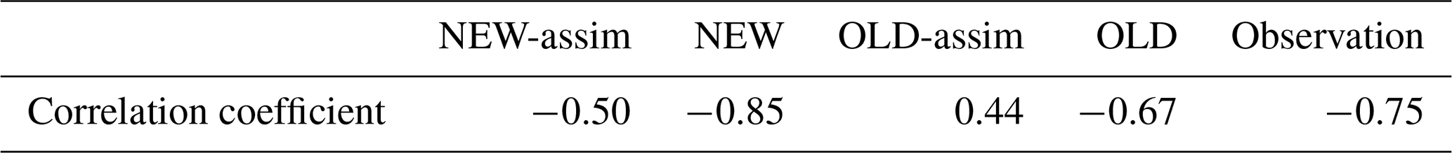
Horizontal maps of the correlation coefficients between simulated and observed CO2F values are shown in Fig. 1. The model output data were the ensemble mean and were linearly interpolated into the SOM-FFN grid. Note that the data were not detrended, and a 1-year running mean filter is applied to the monthly COF2 anomalies in the 1982–2005 period before calculating the correlation coefficients in accordance with the period for which the SOM-FFN dataset is available. CO2F in NEW-assim shows a positive correlation with SOM-FFN in the equatorial Pacific region (Fig. 1a) where significant interannual variations in CO2F are found (Fig. S1). On the other hand, CO2F in OLD-assim (Fig. 1c) is negatively correlated in the equatorial Pacific. The time series in the Niño3 region of both the 1-year running mean SST (hereafter, NINO3-SST) and CO2F (hereafter, NINO3-CO2F) anomalies simulated with NEW-assim (OLD-assim) are shown in Fig. 1b (Fig. 1d). Here, the data were detrended and monthly anomalies were calculated with respect to the 1971–2000 monthly mean climatology. The correlation coefficients between NINO3-SST and NINO3-CO2F anomalies in NEW-assim, OLD-assim, and the observations are −0.50, 0.44, and −0.75, respectively (Table 1). The results in NEW-assim are consistent with the observations, whereas those in OLD-assim are not. The correlation coefficients between the NINO3-SST and NINO3-CO2F anomalies in NEW and OLD are −0.85 and −0.67, respectively (Table 1 and Fig. S2). Note that OLD could capture the observed anticorrelated relationship between the NINO3-SST and NINO3-CO2F anomalies, but OLD-assim could not reproduce this relationship.
Table 1Correlation coefficients between the detrended 1-year running mean NINO3-SST and NINO3-CO2F anomalies in NEW-assim, NEW, OLD-assim, OLD, and the observations. The correlations coefficients in NEW-assim, NEW, OLD-assim, and OLD are for the period from 1961 to 2005 (Figs. 1 and S2), and the correlations coefficient in the observations is for the period from 1982 to 2005.
As the vertical direction of CO2F is determined mainly by pCO2 at the sea surface (see Eq. 2), we further estimated each term in Eq. (3) for each model output (Fig. 2). ∂pCO in the C(X) term in Eq. (3) (X=T, S, DIC, or Alk) was estimated based on the climatological annual mean T, S, DIC, and Alk at the sea surface within the Niño3 region in each experiment. ΔX in C(X) (ΔpCO2 on the left-hand side of Eq. 3) is the variation in X (pCO2) associated with ENSO and was calculated by averaging the monthly mean X (pCO2) anomalies regressed on the NINO3-SST anomalies over the entire Niño3 region. Note that the NINO3-SST anomalies are standardized by the standard deviation. In the following, we describe the anomalies during El Niño periods, whereas the opposite applies during La Niña periods. In NEW-assim, NEW, and OLD, pCO2 decreases because the effect of the decrease in pCO2 with decreasing DIC concentrations is larger than that of the increase in pCO2 with warming (Fig. 2). In OLD-assim, however, the effect of the increase in pCO2 with warming is larger than that of OLD, and the decrease in pCO2 with decreasing DIC concentrations is smaller than that of OLD, resulting in an increase in pCO2. As noted in Sect. 1, previous studies (Le Borgne et al., 2002; Feely et al., 2004; Doney et al., 2009a, b) have shown that the variability in the upwelling during ENSO events dominates the equatorial Pacific CO2F variations through its regulation of DIC. In the following, we discuss the temperature and vertical velocity changes associated with ENSO along the Equator.
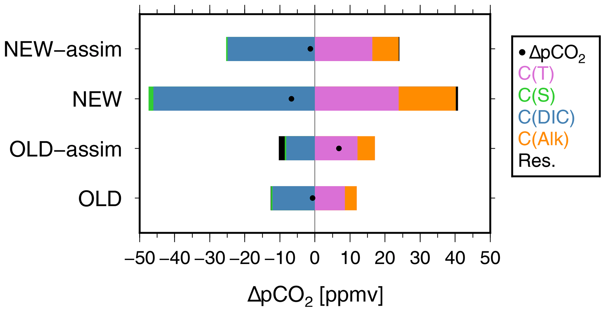
Figure 2Changes in pCO2 regressed onto the standardized NINO3-SST anomalies (ΔpCO2) (dots) and its decomposition with changes in X (X=T, S, DIC, Alk), C(X), and Res. (Eq. 3) evaluated in NEW-assim, NEW, OLD-assim, and OLD. See the text for details regarding the calculation of ΔpCO2, C(X), and Res.
3.2 DIC and vertical velocity changes
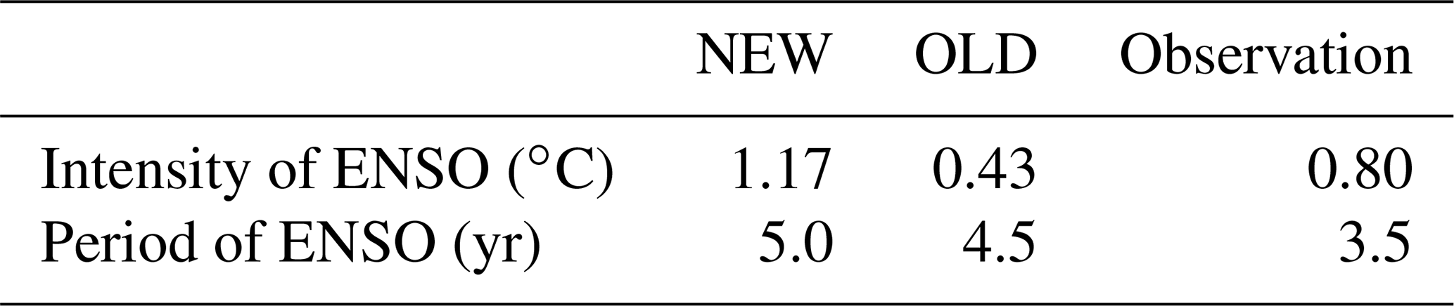
A cross section of the monthly ocean temperature anomalies regressed onto the standardized monthly mean NINO3-SST anomalies along the equatorial Pacific is presented in Figs. 3 and S3 in addition to the climatological annual mean depths of the 18, 20, and 22 ∘C isotherms. Here, monthly temperature anomalies were calculated with respect to the 1971–2000 monthly mean climatology. The observational temperature anomalies and the climatological isotherms are derived from the monthly objective analysis of ocean temperature (Ishii and Kimoto, 2009). Amplitudes of the positive (negative) equatorial temperature anomalies in the upper (lower) layer of the eastern (western) equatorial Pacific in NEW are larger than in OLD and are closer to the observations. The intensity of ENSO, defined as the standard deviation of detrended 1-year running mean NINO3-SST anomalies from 1961 to 2005, is shown in Table 2. The intensity of ENSO in NEW is estimated to be 1.17 ∘C (Table 2), which is a bit stronger than the observed value (0.80 ∘C). On the other hand, the intensity of ENSO in OLD is 0.43 ∘C, which is about half as large as the observed value. In addition, the climatological mean thermocline in NEW is tighter than in OLD and is closer to the observations. The improvement in ENSO reproducibility in NEW is mainly attributed to two updates in the model configuration. The first is the implementation of an updated plume model for cumulus convection with multiple cloud types where the lateral entrainment rate varies vertically depending on the surrounding environment (Chikira and Sugiyama, 2010). The state-dependent lateral entrainment affects the strength of the convectively induced coupled air–sea processes in the eastern tropical Pacific and, thus, the ENSO amplitude in the model. More details are described in Watanabe et al. (2010). The second is the reduction of numerical diffusion due to the introduction of a highly accurate tracer advection scheme in the ocean and an increase in the vertical resolution (Prather, 1986). The equatorial thermocline in the climatic-mean state of the tropical Pacific is more diffuse in OLD than in the observations, which is partly due to numerical diffusion, especially in vertical advection (Tatebe and Hasumi, 2010), and this model bias is much alleviated in NEW. Correspondingly, the so-called “thermocline mode” (e.g., Imada and Kimoto, 2006) becomes more effective and the ENSO amplitude becomes larger in NEW. As the ENSO amplitude in NEW is larger than in OLD, the variation in the equatorial trade winds, which causes anomalous equatorial vertical velocity, is also larger in NEW.
Table 2The intensity and period of ENSO in NEW, OLD, and the observations calculated from the 1-year running mean NINO3-SST anomalies for the period from 1961 to 2005.
To assess the variations in zonal wind associated with ENSO, we estimated the 10 m zonal wind anomalies over the NINO4 region (5∘ S–5∘ N, 160∘ E–150∘ W; the dotted boxes in Fig. 1a) which are regressed onto the NINO3-SST anomalies (Table 3). The Niño4 region is the region of maximum variability for the equatorial trade winds (Fig. S4). Hereafter, the abovementioned regression coefficient is referred to as wind feedback (Guilyardi et al., 2006). The positive value of the wind feedback in NEW (0.92 m s−1 K−1) indicates westerly wind anomalies during El Niño, and this is consistent with the observational dataset, i.e., 1.02 m s−1 K−1. The wind feedback in OLD (0.46 m s−1 K−1) is about half of that in NEW and the observations, respectively.
Table 3The wind feedback and the vertical velocity feedback in NEW-assim, NEW, OLD, and OLD-assim. The wind feedback is computed as the monthly 10 m zonal wind anomalies in the Niño4 region regressed onto the monthly NINO3-SST anomalies, and the vertical velocity feedback is the monthly vertical velocity anomalies at the depth of the 20 ∘C isotherm in the Niño3 region regressed onto the monthly NINO3-SST anomalies. The wind feedback is also evaluated from the observation dataset.

NA: not available.
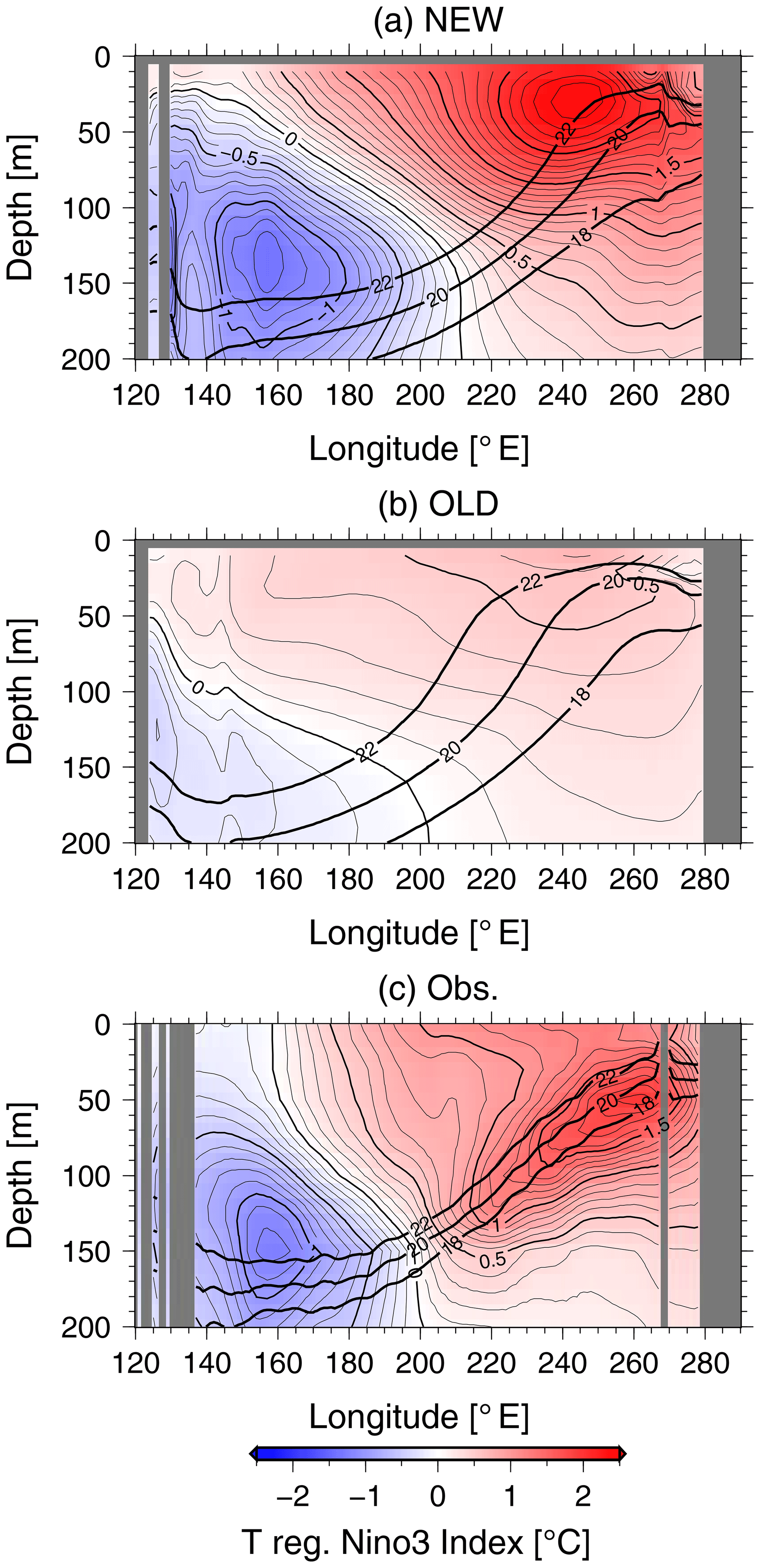
Figure 3Anomalies of equatorial ocean temperature regressed onto the standardized NINO3-SST anomalies for NEW (a), OLD (b), and the observations (c). The contour interval is 0.1 ∘C. The thick solid lines indicate the climatological-mean of the 18, 20, and 22 ∘C isotherms.
Cross sections of the monthly upward water velocity and DIC concentration anomalies along the Equator regressed onto the standardized NINO3-SST anomalies in NEW (OLD) are shown in Fig. 4a and c (Fig. 4b and d), respectively. By reproducing wind feedback that is consistent with the observations, the westerly wind anomalies during El Niño periods in NEW (Fig. S4c) are comparable to that of the JRA-55 reanalysis (Fig. S4i), leading to a weakening of the upward vertical velocity of approximately m s−1 (Fig. 4a). This weakening of the upward vertical velocity causes a decrease in the surface DIC in the eastern equatorial Pacific during El Niño periods (Fig. 4c). In OLD, the smaller wind feedback and the associated smaller westerly wind anomalies than in the JRA-55 reanalysis (Fig. S4g) lead to a weakening of the upward vertical velocity of just 10−6 m s−1 in the equatorial Pacific (Fig. 4b). Although the ENSO signal in OLD is weaker than in the observations, due to a decrease in the upward vertical velocity compared with normal years, the surface DIC concentration decreases during El Niño periods (Fig. 4d). This is consistent with Dong et al. (2016) and shows that OLD is able to qualitatively reproduce the negative correlation between the SST and DIC concentration anomalies in the eastern equatorial Pacific (Fig. S2b).

Figure 4Anomalies of the equatorial vertical velocity (a, b) and DIC (c, d) regressed onto the standardized NINO3-SST anomalies for NEW (a, c) and OLD (b, d). Contour intervals are 0.5 × 10⁻⁶ m s−1 in panels (a) and (b) and 2 μmol L−1 in panels (c) and (d). The thick solid lines indicate the climatological mean of the 18, 20, and 22 ∘C isotherms.
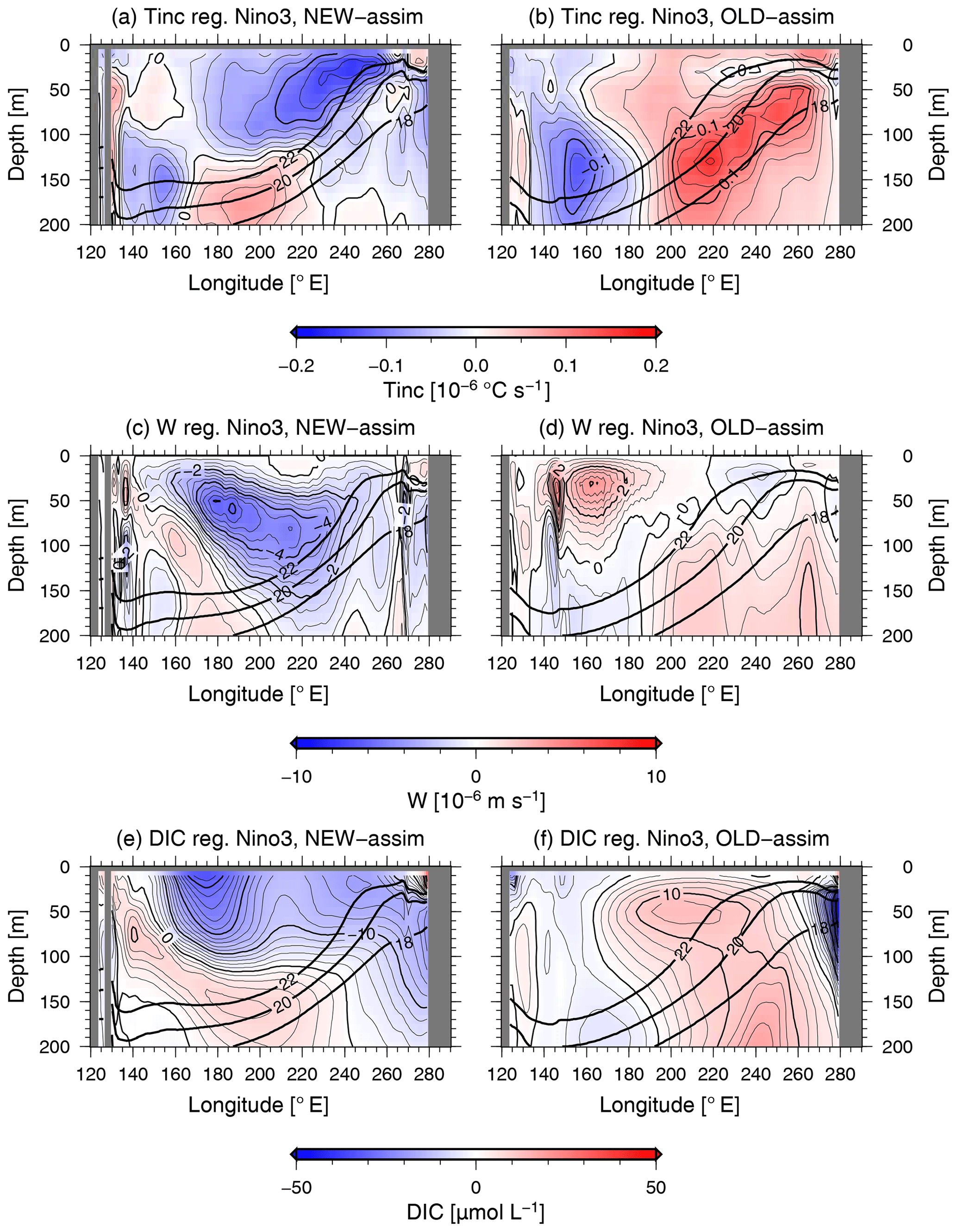
Figure 5Equatorial temperature analysis increments (a, b), vertical velocity anomalies (c, d), and DIC anomalies (e, f) regressed onto the standardized NINO3-SST anomalies for NEW-assim (a, c, e) and OLD-assim (b, d, f). The contour intervals are 0.02 × 10⁻⁶ ∘C s−1 in panels (a) and (b), 0.5 × 10⁻⁶ m s−1 in panels (c) and (d), and 2 µmol L−1 in panels (e) and (f). The thick solid lines indicate the climatological mean of the 18, 20, and 22 ∘C isotherms.
Next, we examined the correction term in temperature due to the data assimilation, i.e., the temperature analysis increment; the final term on the right-hand side of Eq. (1); and the variations in vertical velocity and DIC concentration. Anomalies of the monthly mean temperature analysis increments, the vertical velocity, and the DIC concentration along the Equator regressed onto the standardized NINO3-SST anomalies are shown in Fig. 5. The maximum absolute value of the equatorial temperature analysis increment in NEW-assim is found at depths of 10–40 m in the eastern equatorial Pacific, which is shallower than the depth of the thermocline (Fig. 5a). In NEW-assim, the wind feedback is 0.92 m s−1 K−1 (Table 3), which is of the same magnitude as that in NEW (0.92 m s−1 K−1), and the surface wind anomalies still show a similar pattern to that in NEW (Fig. S4a–d). The westerly wind anomalies in NEW-assim lead to a weakening of the upward vertical velocity along the Equator during El Niño periods (Fig. 5c). To assess the variation in the equatorial vertical velocity associated with ENSO, we estimated the anomalies of the vertical velocity at the depth of the 20 ∘C isotherm (the depth of the thermocline) in the Niño3 region which are then regressed onto the NINO3-SST anomalies. Hereafter, the regression coefficient is referred to as the vertical velocity feedback. The vertical velocity feedback in NEW-assim is estimated to be m s−1 K−1, which is not significantly different from that in NEW (−3.9 × 10⁻⁷ m s−1 K−1) (Table 3). The negative value of the vertical velocity feedback in NEW-assim indicates a weakening of the upward vertical velocity at the depth of the thermocline during El Niño periods in the eastern equatorial Pacific (Fig. 5c). The weakening of the upward vertical velocity causes a decrease in the supply of DIC-rich subsurface water to the surface layer, leading to a reduction in the surface DIC concentration (Fig. 5e). In OLD, the temperature variations associated with ENSO at the depth of the thermocline in the eastern equatorial Pacific are smaller than observed (see Fig. 3b and c), so that the correction term forces a 0.16 × 10⁻⁶ ∘C s−1 increase in the equatorial water temperature during El Niño periods in order to realize the observed temperature variations (Figs. 5b, S3b). The wind feedback in OLD-assim is 0.48 m s−1 K−1 (Table 3), which is the same as in OLD, and the map of the wind speed anomalies shows a similar pattern to that of OLD (Fig. S4e–h); however, the warming due to the data assimilation procedure during El Niño periods reduces the density, leading to low-pressure anomalies. This results in anomalous cyclonic circulation and convergence and, thus, an enhancement of the upward vertical velocity at the depth of the thermocline (Fig. 5d). The vertical velocity feedback in OLD-assim is 4.1 × 10⁻⁷ m s−1 K−1, which has an opposite sign to that in OLD, −4.9 × 10⁻⁷ m s−1 K−1 (Table 3). A positive value of the vertical velocity feedback indicates the enhancement of the upward vertical velocity at the depth of the thermocline during El Niño periods, which is inconsistent with the observations. This spurious enhancement of the upward vertical velocity during El Niño periods causes an increase in the surface DIC concentration (Fig. 5f), leading to a positive correlation between the SST and CO2F (Fig. 1d), contrary to observations. We have to note here that the vertical velocity distribution (Fig. 5c) is even different from NEW in NEW-assim due to the temperature analysis increment (Fig. 4a). As already discussed, the intensity of ENSO in NEW is slightly stronger than observed (Table 2). In addition, the period of ENSO, which is defined as the peak of the power spectrum of the 1-year running mean NINO3-SST, is 5.0 years in NEW, which is longer than the 3.5 years in the observations (see Table 2). Because the ENSO characteristics in NEW are not perfectly consistent with observations, the model nature, namely the responses of the vertical velocity and DIC concentration in ENSO, are still distorted by the temperature analysis increment, even in NEW-assim. This indicates that further model improvements are needed.
In the present study, comparing the results of two ESMs in which observed ocean hydrographic data are assimilated, we have clarified that the representation of the processes in the equatorial climate system is important to reproduce the observed anticorrelated relationship between the SST and CO2F in the equatorial Pacific. When the ocean temperature and salinity observations were assimilated into an ESM with weaker ENSO amplitude than the observations, the correction term in the governing equation of the ocean temperature, which was introduced in the data assimilation procedure, caused spurious upwelling (downwelling) anomalies along the Equator during El Niño (La Niña) periods, leading to an increased (decreased) supply of DIC-rich subsurface water to the surface layer. Due to the resultant increase (decrease) in the surface DIC concentration, the upward (downward) CO2F anomalies during El Niño (La Niña) periods were induced, which was inconsistent with observation. When the ocean temperature and salinity observations were assimilated into the other ESM with a rather realistic ENSO representation, the anticorrelated relationship between the SST and CO2F was reproduced.
Focusing on the CO2F fluctuations associated with ENSO in the equatorial Pacific, Dong et al. (2016) analyzed the results of the CMIP5 ESMs. They showed that only a portion of CMIP5 ESMs (including MIROC-ESM) could reproduce the observed anticorrelated relationship between the SST and CO2F. Bellenger et al. (2014) evaluated the reproducibility of ENSO in the CMIP5 models. They reported that most CMIP5 climate models and ESMs underestimate the amplitude of the wind stress feedback by 20 %–50 % and that only 20 % of CMIP5 models have a relative error within 25 % of the observed value. There are many ESMs where the ENSO characteristics and/or the SST–CO2F relationships are inconsistent with observations. Causes of this discrepancy should be addresses in future studies using methods such as multi-model analysis; moreover, process-based uncertainty estimation will also be required in initialized climate and carbon predictions as well as projections by ESMs.
The model outputs of MIROC-ES2L (Hajima et al., 2019) are available from the the Earth System Grid Federation (ESGF; https://doi.org/10.22033/ESGF/CMIP6.5602). The model outputs of MIROC-ESM (Watanabe et al., 2011) are also available from ESGF (https://esgf-node.llnl.gov/projects/cmip5/, last access: 18 March 2020). The CMIP6 forcing data (Eyring et al., 2016) are version 6.2.1, and the CMIP5 (Taylor et al., 2012) forcing data are described at https://pcmdi.llnl.gov/mips/cmip5/forcing.html, last access: 12 December 2016. The SOM-FFN dataset (Landschützer et al., 2016, 2017) is available at https://www.ncei.noaa.gov/access/ocean-carbon-data-system/oceans/SPCO2_1982_2015_ETH_SOM_FFN.html, last access: 6 June 2019. The JRA-55 reanalysis wind dataset (Kobayashi et al., 2015) is available at https://jra.kishou.go.jp/JRA-55/index_en.html, last access: 1 December 2017. The COBE-SST2 dataset (Ishii et al., 2005; Hirahara et al., 2014) is available at https://www.esrl.noaa.gov/psd/data/gridded/data.cobe2.html, last access: 15 April 2020. The post-processing scripts used for this research and the data used in the figures can be obtained online (https://osf.io/mpk52, Watanabe et al., 2020, last access: 17 November 2020).
The supplement related to this article is available online at: https://doi.org/10.5194/os-16-1431-2020-supplement.
MiW, HT, MaW, and MK contributed to the experimental design. MiW and HK embedded the ocean data assimilation system into the ESMs. MiW and TH performed the experimental simulations. MiW analyzed the model output and drafted the paper. All authors discussed the results, and commented on and edited the paper.
The authors declare that they have no conflict of interest.
We thank Benjamin Barton, Jenny Jardine, Marta Payo Payo, Chris Unsworth, and one anonymous reader for helpful comments. We also thank the three anonymous reviewers, who provided many helpful suggestions for improving the article.
This research has been supported by the Integrated Research Program for Advanced Climate Models (TOUGOU) of the Ministry of Education, Culture, Sports, Science and Technology, MEXT, Japan (grant nos. JPMXD0717935457 and JPMXD0717935715).
This paper was edited by Mario Hoppema and reviewed by three anonymous referees.
Bakker, D. C. E., Pfeil, B., Landa, C. S., Metzl, N., O'Brien, K. M., Olsen, A., Smith, K., Cosca, C., Harasawa, S., Jones, S. D., Nakaoka, S., Nojiri, Y., Schuster, U., Steinhoff, T., Sweeney, C., Takahashi, T., Tilbrook, B., Wada, C., Wanninkhof, R., Alin, S. R., Balestrini, C. F., Barbero, L., Bates, N. R., Bianchi, A. A., Bonou, F., Boutin, J., Bozec, Y., Burger, E. F., Cai, W.-J., Castle, R. D., Chen, L., Chierici, M., Currie, K., Evans, W., Featherstone, C., Feely, R. A., Fransson, A., Goyet, C., Greenwood, N., Gregor, L., Hankin, S., Hardman-Mountford, N. J., Harlay, J., Hauck, J., Hoppema, M., Humphreys, M. P., Hunt, C. W., Huss, B., Ibánhez, J. S. P., Johannessen, T., Keeling, R., Kitidis, V., Körtzinger, A., Kozyr, A., Krasakopoulou, E., Kuwata, A., Landschützer, P., Lauvset, S. K., Lefèvre, N., Lo Monaco, C., Manke, A., Mathis, J. T., Merlivat, L., Millero, F. J., Monteiro, P. M. S., Munro, D. R., Murata, A., Newberger, T., Omar, A. M., Ono, T., Paterson, K., Pearce, D., Pierrot, D., Robbins, L. L., Saito, S., Salisbury, J., Schlitzer, R., Schneider, B., Schweitzer, R., Sieger, R., Skjelvan, I., Sullivan, K. F., Sutherland, S. C., Sutton, A. J., Tadokoro, K., Telszewski, M., Tuma, M., van Heuven, S. M. A. C., Vandemark, D., Ward, B., Watson, A. J., and Xu, S.: A multi-decade record of high-quality fCO2 data in version 3 of the Surface Ocean CO2 ATlas (SOCAT), Earth Syst. Sci. Data, 8, 383–413, https://doi.org/10.5194/essd-8-383-2016, 2016.
Bellenger, H., Guilyardi, E., Leloup, J., Lengaigne, M., and Vialard, J.: ENSO representation in climate models: From CMIP3 to CMIP5, Clim. Dynam., 42, 1999–2018, https://doi.org/10.1007/s00382-013-1783-z, 2014.
Bloom, S. C., Takacs, L. L., da Silva, A. M., and Ledvina, D.: Data assimilation using incremental analysis updates, Mon. Weather Rev., 124, 1256–1271, 1996.
Brasseur, P., Gruber, N., Barciela, R., Brander, K., Doron, M., El Moussaoui, A., Hobday, A. J., Huret, M., Kremeur, A.-S., Lehodey, P., Matear, R., Moulin, C., Murtugudde, R., Senina, I., and Svendsen, E.: Integrating biogeochemistry and ecology into ocean data assimilation systems, Oceanography, 22, 206–215, https://doi.org/10.5670/oceanog.2009.80, 2009.
Chikira, M. and Sugiyama, M.: A cumulus parameterization with state-dependent entrainment rate, Part I: Description and sensitivity to temperature and humidity profiles, J. Atmos. Sci., 67, 2171–2193, https://doi.org/10.1175/2010JAS3316.1, 2010.
Doney, S. C., Bopp, L., and Long, M. C.: Historical and future trends in ocean climate and biogeochemistry, Oceanography, 27, 108–119, https://doi.org/10.5670/oceanog.2014.14, 2014.
Doney, S. C., Balch, W. M., Fabry, V. J., and Feely, R. A.: Ocean acidification: A critical emerging problem for the ocean sciences, Oceanography, 22, 16–25, https://doi.org/10.5670/oceanog.2009.93, 2009a.
Doney, S. C., Fabry, V. J., Feely, R. A., and Kleypas, J. A.: Ocean acidification: The other CO2 problem, Annu. Rev. Mar. Sci., 1, 169–192, https://doi.org/10.1146/annurev.marine.010908.163834, 2009b.
Dong, F., Li, Y., Wang, B., Huang, W., Shi, Y., and Dong, W.: Global air–sea CO2 flux in 22 CMIP5 models: Multiyear mean and interannual variability, J. Clim., 29, 2407–2431, https://doi.org/10.1175/JCLI-D-14-00788.1, 2016.
Dong, F., Li, Y., and Wang, B.: Assessment of responses of Tropical Pacific air–sea CO2 flux to ENSO in 14 CMIP5 models, J. Clim., 30, 8595–8613, https://doi.org/10.1175/JCLI-D-16-0543.1, 2017.
Eyring, V., Bony, S., Meehl, G. A., Senior, C. A., Stevens, B., Stouffer, R. J., and Taylor, K. E.: Overview of the Coupled Model Intercomparison Project Phase 6 (CMIP6) experimental design and organization, Geosci. Model Dev., 9, 1937–1958, https://doi.org/10.5194/gmd-9-1937-2016, 2016.
Feely, R. A., Wanninkhof, R., Goyet, C., Archer, D. E., and Takahashi, T.: Variability of CO2 distributions and sea–air fluxes in the central and eastern equatorial Pacific during the 1991–1994 El Niño, Deep-Sea Res. II, 44, 1851–1867, https://doi.org/10.1016/S0967-0645(97)00061-1, 1997.
Feely, R. A., Wanninkhof, R., Takahashi, T., and Tans, P.: Influence of El Niño on the equatorial Pacific contribution to atmospheric CO2 accumulation, Nature, 398, 597–601, https://doi.org/10.1038/19273, 1999.
Feely, R. A., Wanninkhof, R., McGillis, W., Carr, M.-E., and Cosca, C. E.: Effects of wind speed and gas exchange parameterizations on the air–sea CO2 fluxes in the equatorial Pacific Ocean, J. Geophys. Res., 109, C08S03, https://doi.org/10.1029/2003JC001896, 2004.
Gill, A. E.: Some simple solutions for heat-induced tropical circulation, Q. J. Roy. Meteorol. Soc., 106, 447–462, 1980.
Guilyardi, E, Braconnot, P., Jin, F.-F., Kim, S. T., Kolasinski, M., Li, T., and Musat, I.: Atmosphere feedbacks during ENSO in a coupled GCM with a modified atmospheric convection scheme, J. Clim., 22, 5698–5718, https://doi.org/10.1175/2009JCLI2815.1, 2009.
Hajima, T., Abe, M., Arakawa, O., Suzuki, T., Komuro, Y., Ogura, T., Ogochi, K., Watanabe, M., Yamamoto, A., Tatebe, H., Noguchi, M. A., Ohgaito, R., Ito, A., Yamazaki, D., Ito, A., Takata, K., Watanabe, S., Kawamiya, M., and Tachiiri, K.: MIROC MIROC-ES2L model output prepared for CMIP6 CMIP historical, Earth System Grid Federation, Version: 20191118, https://doi.org/10.22033/ESGF/CMIP6.5602, 2019.
Hajima, T., Watanabe, M., Yamamoto, A., Tatebe, H., Noguchi, M. A., Abe, M., Ohgaito, R., Ito, A., Yamazaki, D., Okajima, H., Ito, A., Takata, K., Ogochi, K., Watanabe, S., and Kawamiya, M.: Development of the MIROC-ES2L Earth system model and the evaluation of biogeochemical processes and feedbacks, Geosci. Model Dev., 13, 2197–2244, https://doi.org/10.5194/gmd-13-2197-2020, 2020.
Hirahara, S., Ishii, M., and Fukuda, Y.: Centennial-scale sea surface temperature analysis and its uncertainty, J. Clim., 27, 57–75, https://doi.org/10.1175/JCLI-D-12-00837.1, 2014.
Huang, B., Kinter, J. L., and Schopf, P. S.: Ocean data assimilation using intermittent analyses and continuous model error correction, Adv. Atmos. Sci., 19, 965–992, https://doi.org/10.1007/s00376-002-0059-z, 2002.
Imada, Y. and Kimoto, M.: Improvement of thermocline structure that affect ENSO performance in a coupled GCM, SOLA 2, 164–167, https://doi.org/10.2151/sola.2006-042, 2006.
IPCC: Climate change 2013: The physical science basis, in: Contribution of Working Group I to the Fifth Assessment Report of the Intergovernmental Panel on Climate Change, edited by: Stocker, T. F., Qin, D., Plattner, G.-K., Tignor, M., Allen, S. K., Boschung, J., Nauels, A., Xia, Y., Bex, V., and Mdgley, P. M., Cambridge University Press, Cambridge, UK, New York, NY, USA, p. 1535, 2013.
Ishii, M. and Kimoto, M.: Reevaluation of historical ocean heat content variations with time-varying XBT and MBT depth bias corrections, J. Oceanogr., 65, 287–299, https://doi.org/10.1007/s10872-009-0027-7, 2009.
Ishii, M., Shouji A., Sugimoto, S., and Matsumoto, T.: Objective analyses of sea-surface temperature and marine meteorological variables for the 20th century using ICOADS and the Kobe Collection, Int. J. Climatol., 25, 865–879, https://doi.org/10.1002/joc.1169, 2005.
Jones, C. D., Collins, M., Cox, P. M., and Spall, S. A.: The carbon cycle response to ENSO: A coupled climate–carbon cycle model study, J. Clim., 14, 4113–4129, https://doi.org/10.1175/1520-0442(2001)014<4113:TCCRTE>2.0.CO;2, 2001.
K-1 model developers: K-1 coupled GCM (MIROC) description, K-1 Tech. Rep., 1, edited by: Hasumi, H. and Emori, S., Center for Climate System Research, the Univ. of Tokyo, Tokyo, 34 pp., 2004.
Kawamiya, M., Hajima, T., Tachiiri, K., Watanabe, S., and Yokohata, T.: Two decades of Earth system modeling with an emphasis on Model for Interdisciplinary Research on Climate (MIROC), Prog. Earth Planet Sci., 7, 64, https://doi.org/10.1186/s40645-020-00369-5, 2020.
Keeling, C. D. and Revelle, R.: Effects of El Niño/Southern Oscillation on the atmospheric content of carbon dioxide, Meteoritics, 20, 437–450, 1985.
Keenlyside, N. S., Latif, M., Jungclaus, J., Kornblueh, L., and Roeckner, E.: Advancing decadal-scale climate prediction in the North Atlantic sector, Nature, 453, 84–88, https://doi.org/10.1038/nature06921, 2008.
Kobayashi, S., Ota, Y., Harada, Y., Ebita, A., Moriya, M., Onoda, H., Onogi, K., Kamahori, H., Kobayashi, C., Endo, H., Miyaoka, K., and Takahashi, K.: The JRA-55 Reanalysis: General specifications and basic characteristics, J. Meteorol. Soc. Jap., 93, 5–48, https://doi.org/10.2151/jmsj.2015-001, 2015.
Landschützer, P., Gruber, N., Bakker, D. C. E., and Schuster, U.: Recent variability of the global ocean carbon sink, Global Biogeochem. Cy., 28, 927–949, https://doi.org/10.1002/2014GB004853, 2014.
Landschützer, P., Gruber, N., and Bakker, D. C. E.: Decadal variations and trends of the global ocean carbon sink, Global Biogeochem. Cy., 30, 1396–1417, https://doi.org/10.1002/2015GB005359, 2016.
Landschützer, P., Gruber, N., and Bakker, D. C. E.: An updated observation-based global monthly gridded sea surface pCO2 and air-sea CO2 flux product from 1982 through 2015 and its monthly climatology (NCEI Accession 0160558), Version 2.2, NOAA National Centers for Environmental Information, Dataset, 2017.
Landschützer, P., Gruber, N., Bakker, D. C. E., Stemmler, I., and Six, K. D.: Strengthening seasonal marine CO2 variations due to increasing atmospheric CO2, Nat. Clim. Change, 8, 146–150, https://doi.org/10.1038/s41558-017-0057-x, 2018.
Le Borgne, R., Feely, R. A., and Mackey, D. J.: Carbon fluxes in the equatorial Pacific: A synthesis of the JGOFS programme, Deep-Sea Res. Pt. II, 49, 2425–2442, https://doi.org/10.1016/S0967-0645(02)00043-7, 2002.
Le Quéré, C., Raupach, M. R., Canadell, J. G., Marland, G., Bopp, L., Ciais, P., Conway, T. J., Doney, S. C., Feely, R. A., Foster, P., Friedlingstein, P., Gurney, K., Houghton, R. A., House, J. I., Hungintford, C., Levy, P. E., Lomas, M. R., Majkut, J., Metzl, N., Ometto, J. P., Peters, G. P., Prentice, I. C., Randerson, J. T., Running, S. W., Sarmiento, J. L., Schuster, U., Sitch, S., Takahashi, T., Viovy, N., van der Werf, G. R., and Woodward, F. I.: Trends in the sources and sinks of carbon dioxide, Nat. Geosci., 2, 831–836, https://doi.org/10.1038/ngeo689, 2009.
Le Quéré, C., Takahashi, T., Buitenhuis, E. T., Rödenbeck, C., and Sutherland, S. C.: Impact of climate change and variability on the global oceanic sink of CO2, Global Biogeochem. Cy., 24, GB4007, https://doi.org/10.1029/2009GB003599, 2010.
Le Quéré, C., Andrew, R. M., Canadell, J. G., Sitch, S., Korsbakken, J. I., Peters, G. P., Manning, A. C., Boden, T. A., Tans, P. P., Houghton, R. A., Keeling, R. F., Alin, S., Andrews, O. D., Anthoni, P., Barbero, L., Bopp, L., Chevallier, F., Chini, L. P., Ciais, P., Currie, K., Delire, C., Doney, S. C., Friedlingstein, P., Gkritzalis, T., Harris, I., Hauck, J., Haverd, V., Hoppema, M., Klein Goldewijk, K., Jain, A. K., Kato, E., Körtzinger, A., Landschützer, P., Lefèvre, N., Lenton, A., Lienert, S., Lombardozzi, D., Melton, J. R., Metzl, N., Millero, F., Monteiro, P. M. S., Munro, D. R., Nabel, J. E. M. S., Nakaoka, S., O'Brien, K., Olsen, A., Omar, A. M., Ono, T., Pierrot, D., Poulter, B., Rödenbeck, C., Salisbury, J., Schuster, U., Schwinger, J., Séférian, R., Skjelvan, I., Stocker, B. D., Sutton, A. J., Takahashi, T., Tian, H., Tilbrook, B., van der Laan-Luijkx, I. T., van der Werf, G. R., Viovy, N., Walker, A. P., Wiltshire, A. J., and Zaehle, S.: Global Carbon Budget 2016, Earth Syst. Sci. Data, 8, 605–649, https://doi.org/10.5194/essd-8-605-2016, 2016.
Li, H., Ilyina, T., Müller, W. A., and Sienz, F.: Decadal predictions of the North Atlantic CO2 uptake, Nat. Commun., 7, 11076, https://doi.org/10.1038/ncomms11076, 2016.
Li, H., Ilyina, T., Müller, W. A., and Landschützer, P.: Predicting the variable ocean carbon sink, Sci. Adv., 5, eaav6471, https://doi.org/10.1126/sciadv.aav6471, 2019.
McKinley, G. A., Follows, M. J., and Marshall, J.: Mechanisms of air–sea CO2 flux variability in the equatorial Pacific and the North Atlantic, Global Biogeochem. Cy., 18, GB2011, https://doi.org/10.1029/2003GB002179, 2004.
Mochizuki, T., Ishii, M., Kimoto, M., Chikamoto, Y., Watanabe, M., Nozawa, T., Sakamoto, T. T., Shiogama, H., Awaji, T., Sugiura, N., Toyoda, T., Yasunaka, S., Tatebe, H., and Mori, M.: Pacific decadal oscillation hindcasts relevant to near-term climate prediction, P. Nat. Acad. Sci. USA, 107, 1833–1837, https://doi.org/10.1073/pnas.0906531107, 2010.
Obata, A. and Kitamura, Y.: Interannual variability of the sea–air exchange of CO2 from 1961 to 1998 simulated with a global ocean circulation-biogeochemistry model, J. Geophys. Res., 108, 3337, https://doi.org/10.1029/2001JC001088, 2003.
Park, G.-H., Wanninkhof, R., Doney, S. C., Takahashi, T., Lee, K., Feely, R. A., Sabine, C. L., Triñanes, J., and Lima, I.: Variability of global net sea–air CO2 fluxes over the last three decades using empirical relationships, Tellus B, 62, 352–368, https://doi.org/10.1111/j.1600-0889.2010.00498.x, 2010.
Park, J.-Y., Stock, C. A., Yang, X., Dunne, J. P., Rosati, A., John, J., and Zhang, S.: Modeling global ocean biogeochemistry with physical data assimilation: A pragmatic solution to the Equatorial instability, J. Adv. Model. Earth Syst., 10, 891–906, https://doi.org/10.1002/2017MS001223, 2018.
Patra, P. K., Maksyutov, S., Ishizawa, M., Nakazawa, T., Takahashi, T., and Ukita, J.: Interannual and decadal changes in the sea–air CO2 flux from atmospheric CO2 inverse modeling, Global Biogeochem. Cy., 19, GB4013, https://doi.org/10.1029/2004GB002257, 2005.
Pohlmann, H., Jungclaus, J. H., Köhl, A., Stammer, D., and Marotzke, J.: Initializing decadal climate predictions with the GECCO oceanic synthesis: Effects on the North Atlantic, J. Clim., 22, 3926–3938, https://doi.org/10.1175/2009JCLI2535.1, 2009.
Prather, M. J.: Numerical advection by conservation of second-order moments, J. Geophys. Res., 91, 6671–6681, 1986.
Rödenbeck, C., Bakker, D. C. E., Metzl, N., Olsen, A., Sabine, C., Cassar, N., Reum, F., Keeling, R. F., and Heimann, M.: Interannual sea–air CO2 flux variability from an observation-driven ocean mixed-layer scheme, Biogeosciences, 11, 4599–4613, https://doi.org/10.5194/bg-11-4599-2014, 2014.
Sabine, C. L., Feely, R. A., Gruber, N., Key, R. M., Lee, K., Bullister, J. L., Wanninkhof, R., Wong, C. S., Wallace, D. W. R., Tilbrook, B., Millero, F. J., Peng, T.-H., Kozyr, A., Ono, T., and Rios, A. F.: The oceanic sink for anthropogenic CO2, Science, 305, 367–371, https://doi.org/10.1126/science.1097403, 2004.
Smith, D. M., Cusack, S., Colman, A. W., Folland, C. K., Harris, G. R., and Murphy, J. M.: Improved surface temperature prediction for the coming decade from a global climate model, Science, 317, 796–799, https://doi.org/10.1126/science.1139540, 2007.
Sospedra-Alfonso, R. and Boer, G. J.: Assessing the impact of initialization on decadal prediction skill, Geophys. Res. Lett., 47, GL086361, https://doi.org/1029/2019GL086361, 2020.
Takahashi, T., Olafsson, J., Goddard, J. G., Chipman, D. W., and Sutherland, S. C.: Seasonal variation of CO2 and nutrients in the high-latitude surface oceans: A comparative study, Global Biogeochem. Cy., 7, 843–878, https://doi.org/10.1029/93GB02263, 1993.
Tatebe, H. and Hasumi, H.: Formation mechanism of the Pacific equatorial thermocline revealed by a general circulation model with a high accuracy tracer advection scheme, Ocean Model., 35, 245–252, 2010.
Tatebe, H., Ishii, M., Mochizuki, T., Chikamoto, Y., Sakamoto, T. T., Komuro, Y., Mori, M., Yasunaka, S., Watanabe, M., Ogochi, K., Suzuki, T., Nishimura, T., and Kimoto, M.: The initialization of the MIROC climate models with hydrographic data assimilation for decadal prediction, J. Meteorol. Soc. Jpn. Pt. A, 90, 275–294, https://doi.org/10.2151/jmsj.2012-A14, 2012.
Tatebe, H., Tanaka, Y., Komuro, Y., and Hasumi, H.: Impact of deep ocean mixing on the climatic mean state in the Southern Ocean, Sci. Rep., 8, 14479, https://doi.org/10.1038/s41598-018-32768-6, 2018.
Taylor, K. E., Stouffer, R. J., and Meehl, G. A.: An overview of CMIP5 and the experiment design, Bull. Am. Meteorol. Soc., 93, 485–498, https://doi.org/10.1175/BAMS-D-11-00094.1, 2012.
Tommasi, D., Stock, C. A., Hobday, A. J., Methot, R., Kaplan, I. C., Eveson, J. P., Holsman, K., Miller, T. J., Gaichas, S., Gehlen, M., Pershing, A., Vecchi, G. A., Msadek, R., Delworth, T., Eakin, C. M., Haltuch, M. A., Séférian, R., Spillman, C. M., Hartog, J. R., Siedlecki, S., Samhouri, J. F., Muhling, B., Asch, R. G., Pinsky, M. L., Saba, V. S., Kapnick, S. B., Gaitan, C. F., Rykaczewski, R. R., Alexander, M. A., Xue, Y., Pegion, K. V., Lynch, P., Payne, M. R., Kristiansen, T., Lehodey, P., and Werner, F. E.: Managing living marine resources in a dynamic environment: The role of seasonal to decadal climate forecasts, Prog. Oceanogr., 152, 15–49, https://doi.org/10.1016/j.pocean.2016.12.011, 2017a.
Tommasi, D., Stock, C. A., Alexander, M. A., Yang, X., Rosati, A., and Vecchi, G. A.: Multi-annual climate predictions for fisheries: An assessment of skill of sea surface temperature forecasts for large marine ecosystems, Front. Mar. Sci., 4, 201, https://doi.org/10.3389/fmars.2017.00201, 2017b.
United Nations Framework Convention on Climate Change (UNFCCC): Adoption of the Paris Agreement FCCC/CP/2015/L.9/Rev.1 UNFCCC, 2015.
Valsala, V. and Maksyutov, S.: Simulation and assimilation of global ocean pCO2 and air–sea CO2 fluxes using ship observations of surface ocean pCO2 in a simplified biogeochemical offline model, Tellus B, 62, 821–840, https://doi.org/10.1111/j.1600-0889.2010.00495.x, 2010.
Wanninkhof, R.: Relationship between wind speed and gas exchange over the ocean, J. Geophys. Res., 97, 7373–7382, https://doi.org/10.1029/92JC00188, 1992.
Wanninkhof, R.: Relationship between wind speed and gas exchange over the ocean revisited, Limnol. Oceanogr. Method., 12, 351–362, https://doi.org/10.4319/lom.2014.12.351, 2014.
Watanabe, M., Suzuki, T., O'ishi, R., Komuro, Y., Watanabe, S., Emori, S., Takemura, T., Chikira, M., Ogura, T., Sekiguchi, M., Takata, K., Yamazaki, D., Yokohata, T., Nozawa, T., Hasumi, H., Tatebe, H., and Kimoto, M.: Improved climate simulation by MIROC5: Mean states, variability, and climate sensitivity, J. Clim., 23, 6312–6335, https://doi.org/10.1175/2010JCLI3679.1, 2010.
Watanabe, S., Hajima, T., Sudo, K., Nagashima, T., Takemura, T., Okajima, H., Nozawa, T., Kawase, H., Abe, M., Yokohata, T., Ise, T., Sato, H., Kato, E., Takata, K., Emori, S., and Kawamiya, M.: MIROC-ESM 2010: Model description and basic results of CMIP5-20c3m experiments, Geosci. Model Dev., 4, 845–872, https://doi.org/10.5194/gmd-4-845-2011, 2011.
Watanabe, M., Tatebe, H., Koyama, H., Hajima, T., Watanabe, M., and Kawamiya, M.: Importance of El Niño reproducibility for reconstructing historical CO2 flux variations in the equatorial Pacific, OSF, https://osf.io/mpk52, last access: 17 November 2020.
Weiss, R.: Carbon dioxide in water and seawater: The solubility of a non-ideal gas, Mar. Chem., 2, 203–215, https://doi.org/10.1016/0304-4203(74)90015-2, 1974.