the Creative Commons Attribution 4.0 License.
the Creative Commons Attribution 4.0 License.
 | 09 Nov 2020
Bardsey – an island in a strong tidal stream: underestimating coastal tides due to unresolved topography
David T. Pugh
Bardsey Island is located at the western end of the Llŷn Peninsula in northwestern Wales. Separated from the mainland by a channel that is some 3 km wide, it is surrounded by reversing tidal streams of up to 4 m s−1 during spring tides. These local hydrodynamic details and their consequences are unresolved by satellite altimetry and are not represented in regional tidal models. Here we look at the effects of the island on the strong tidal stream in terms of the budgets for tidal energy dissipation and the formation and shedding of eddies. We show, using local observations and a satellite-altimetry-constrained product (TPXO9), that the island has a large impact on the tidal stream and that even in this latest altimetry-constrained product the derived tidal stream is under-represented due to the island not being resolved. The effect of the island leads to an underestimate of the current speed in the TPXO9 data in the channel of up to a factor of 2.5, depending on the timing in the spring–neap cycle, and the average tidal energy resource is underestimated by a factor up to 14. The observed tidal amplitudes are higher at the mainland than at the island, and there is a detectable phase lag in the tide across the island; this effect is not seen in the TPXO9 data. The underestimate of the tide in the TPXO9 data has consequences for tidal dissipation and wake effect computation and shows that local observations are key to correctly estimating tidal energetics around small-scale coastal topography.
- Article
(2468 KB) - Full-text XML
- BibTeX
- EndNote


Scientific understanding of global tidal dynamics is well established. Following the advent of satellite observations, up to 15 tidal constituents have been mapped using altimetry-constrained numerical models, and the resulting products are verified and constrained further using in situ tidal data; see Stammer et al. (2014) for details. There is, however, still an issue in terms of spatial resolution of the altimetry-constrained products: even the most recent (global) tidal models have only 1∕30∘ resolution (equivalent to ∼ 3.2 km in longitude at the Equator, ∼1.9 km in the domain here, and 3.2 km in latitude everywhere). The satellite themselves may have track separation of hundreds of kilometres (Egbert and Erofeeva, 2002), and the coastline can introduce biases in the altimetry data that limit the usefulness of them in the assimilation process. Consequently, smaller topographic features and islands are unresolved and may be “invisible” in altimetry-constrained product even if the features may be resolved in the latest bathymetry databases, e.g. the General Bathymetric Chart of the Oceans (GEBCO, https://www.gebco.net/, last access: 2 November 2020; Jakobsson et al., 2020). This can mean that the tidal energetics in the products, and in other numerical models with insufficient resolution, can be biased because unresolved wakes downstream of the topography can act as a large energy sink (McCabe et al., 2006; Stigebrandt, 1980; Warner and MacCready, 2014). Whilst the globally integrated energetics of these models are consistent with astronomical estimates from lunar recession rates (Bills and Ray, 1999; Egbert and Ray, 2001), the local estimates can be wrong. However, new correction algorithms improve the satellite data near coasts (e.g. Piccioni et al., 2018), but this is yet to be included in global tidal products.
Because many of the altimetry-constrained tidal databases are models, and not altimeter databases, they also provide tidal currents as well as elevations. This is true for TPXO9 (see Egbert and Erofeeva, 2002, and https://www.tpxo.net/, last access: 2 November 2020, for details), the altimetry-constrained product used here. Here, we use a series of tide-gauge measurements from Bardsey Island in the Irish Sea (Fig. 1) alongside TPXO9 to evaluate the effect of the island on the tidal dynamics as they track around Bardsey Island. Bardsey Island is a rocky melange of sedimentary and igneous rocks, including some granites, located 3.1 km off the Llŷn Peninsula in northern Wales, UK (Fig. 1a). It is approximately 1 km wide (though it is only 300 m wide at the narrowest point) and 1.6 km long. It reaches 167 m at its highest point. Bardsey Sound, between the Llŷn peninsula and the island, experiences strong tidal currents. The relatively small scale of the island and the sound means that the local detail is not “seen” in the altimetry-constrained products. The active local tidal dynamics that are uncaptured by the altimetry-constrained data allow us to compare the altimetry-constrained tidal characteristics in TPXO9 for the region with accurate local observations and quantify the validity limits of TPXO9 for this type of investigation. We will make a direct comparison of the tidal amplitudes and phases measured by the bottom pressure gauges around the island; see Fig. 1b for tide gauge (TG) locations and a summary of the in situ tides. We also consider whether (and when in the tidal cycle) flow separation occurs in the wake of the island.
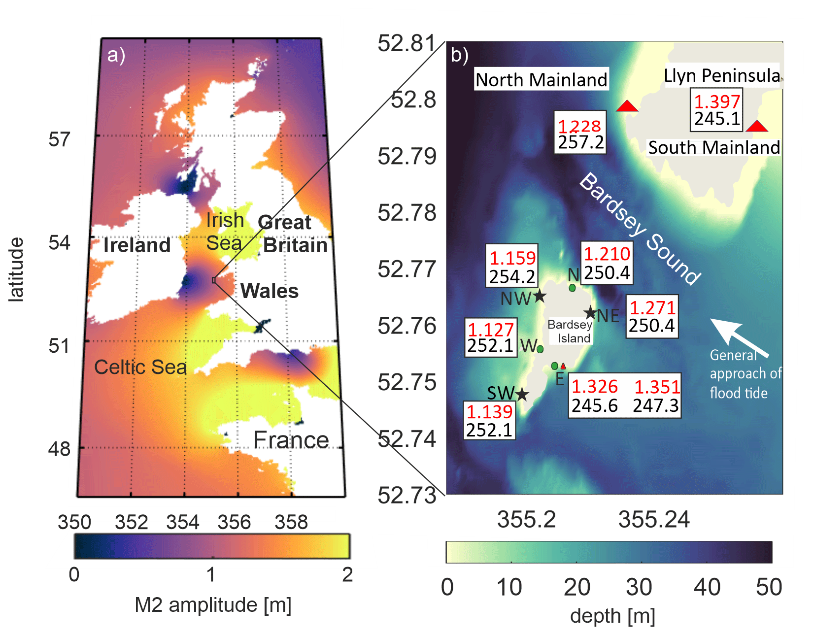
Figure 1(a) Map of the European shelf showing M2 amplitudes in metres, taken from TPXO9. (b) Details of local topography and tidal characteristics in the vicinity of Bardsey Island. The symbols mark the TG location, with green ellipses denoting Deployment 1, black stars denoting Deployment 2, and red triangles denoting Deployment 3. Note that site East was occupied twice, during Deployments 1 and 3. The red numbers in the text boxes are the amplitudes (in metres) and the phase lags on Greenwich (in degrees, one degree is almost 2 min in time) from the harmonic analysis for each tide gauge. The bathymetry comes from EMODnet (https://www.emodnet-bathymetry.eu/, last access: 2 November 2020).
We will use some basic fluid–flow parameters in our analysis later. Transition to turbulence, and hence flow separation around an object, can be parameterized in terms of a Reynolds number, , where U is a velocity scale, D is the size of the object, and ν∼100 is a horizontal diffusivity (see, e.g. Wolanski et al., 1984). It indicates when there is a transition to flow separation behind the island: at low Reynolds numbers, Re<1, the flow is quite symmetric upstream and downstream, and there is no flow separation at the object. As the Reynolds number is increased to the range , laminar separation happens and results in two steady vortices downstream. As Re increases further, up to Re<1000, these steady vortices are replaced by a periodic von Karman vortex street, whereas if Re>1000, there is a fully separated turbulent flow (Kundu and Cohen, 2002).
Another useful non-dimensional number for this type of investigation is the Strouhal number, . Here, f is the frequency of the shedding of vortices. Fully developed vortices are generated when T>f, where T is the frequency of the oscillating flow (Dong et al., 2007; Magaldi et al., 2008). If, on the other hand, the tidal frequency is larger than f, only one wake eddy will be shed on each tidal cycle, if it has time to form at all.
2.1 In situ data collection
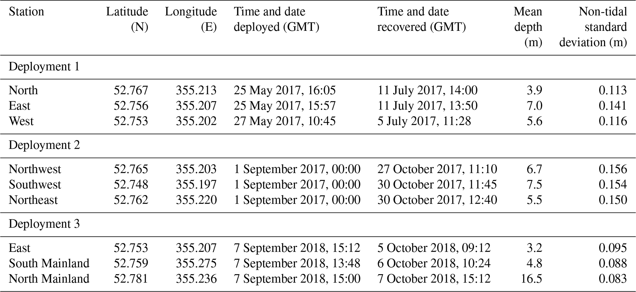
The tidal elevations around Bardsey were measured in three deployments, from summer 2017 through to spring 2018 (Table 1 and Fig. 1b). Site East, the main harbour for the island at Y Cafn, was occupied twice as a control, during Deployments 1 and 3. The other instrument deployments were bottom mounted a few tens of metres laterally offshore, and all instruments were deployed at depths between 3.2 and 16.5 m. The instruments used were pressure recorders from RBR with a measurement resolution better than 0.001 m, and they were set to sample every 6 min.
The resulting pressure series were analysed to extract tides, using the Tidal Analysis Software Kit of the National Oceanographic Centre (NOC, 2020). Analyses were made for 26 constituents, including mean sea level, and eight related constituents, appropriate for a month or more of data (Pugh and Woodworth, 2014). In Table 2 the three constituents listed are the two biggest, M2 and S2, and (as an indicator of the presence of shallow water tides) M4, the first harmonic of M2. Shallow-water tides are enhanced around the island because of the curvature of the flow as it bypasses the island and headland (see Sect. 6.2.3 of Pugh and Woodworth, 2014). The non-tidal residuals, the final column in Table 1, compare well with the residuals at Holyhead, the nearest permanent tide gauge station some 70 km north: for Holyhead these were 0.096, 0.172, and 0.067 m for the same periods (note that bottom pressure measurements at Bardsey include a partial natural sea level compensation for the inverted barometer effect). Deployment 2 residuals at both Bardsey and at Holyhead were noticeably higher than for the other two deployments because Deployment 2 included one of the most severe storms and waves in local memory: Hurricane Ophelia, which had maximum local wind speeds on 16 October 2017. A good indication of the internal quality of the in situ observations and analyses is given by the consistency in the tidal ages and S2∕M2 amplitude ratios. The tidal age is the time after maximum astronomical tidal forcing and the local maximum spring tides, or approximately the phase difference between the phases of S2 and M2 in hours, whereas the amplitude ratios are related to the spring–neap amplitude cycle. These are given in the final columns of Table 2. The effects of the storm were not noticeable in the tidal signals, as they were at very different natural frequencies. The subsurface pressure measurements at Bardsey include atmospheric pressure variations and any tidal variation therein. However, at these latitudes the atmospheric pressure S2 variations are very small. At the Equator the atmospheric S2 has an amplitude of about 1.25 mbar, which decreases away from the Equator as cos 3(latitude), and thus at 53∘ N the amplitude is reduced to 0.26 mbar, a sea level equivalent of 2.5 mm.
Amplitudes and phases of tidal constituents based on short periods of observations need adjusting to reflect the long-term values of amplitudes and phases. The values in Table 2 have been adjusted for both nodal effects and for an observed non-astronomical seasonal modulation of M2. Standard harmonic analyses include an automatic adjustment to amplitudes and phases of lunar components to allow for the full 3.7 %, 18.6-year modulation due to the regression of lunar nodes. However, the full 3.7 % nodal modulation is generally heavily reduced in shallow water and shelf seas, and thus local counter adjustments are needed. The nodal M2 amplitude modulation at Holyhead, the nearest standard port, is reduced to 1.8 % (Woodworth et al., 1991). We have used this value in correcting the standard 3.7 % adjustment. The M4 nodal modulations are twice that for M2. The seasonal M2 modulations are generally observed to have regional coherence, so we have used the seasonal modulations from 9 years of Newlyn data (in the period 2000–2011). M4 is not seasonally adjusted, and S2 is not a lunar term, so it is not nodally modulated. These very precise adjustments are possible and useful, but overall, as stated in the caption to Table 2, for regional comparisons we assume, slightly conservatively, confidence ranges of 1 % for amplitudes and 1.0∘ for phases.
2.2 TPXO9 data
The altimetry-constrained product used in this paper is that of the TPXO9 ATLAS, which is derived from assimilation of both satellite altimeter and tide gauge data into a forward model solution (Egbert and Erofeeva, 2002). The resolution is 1∕30∘ in both latitude and longitude (3.7 and 2.2 km at Bardsey). We used the elevation and transport information and their respective phases for the M2, S2, and M4 constituents. In the following calculations, we approximate the largest tidal current speeds or amplitudes as the sum of the amplitudes of the above three tidal constituents. Of course this is only a crude estimate of the full highest and lowest astronomical tides. Note that we are not allowing for M2 to M4 phase locking, and the relatively small diurnal tides are ignored. We refer to this as the GA (greatest astronomical) in the following.
2.3 LANDSAT data
Landsat-8 data images were used to identify possible eddies in the currents and further illustrate unresolved effects due to the island. Note that we are not aiming for a full wake description in this paper. Data were downloaded from the Earth Explorer website (https://earthexplorer.usgs.gov/, last access: 2 November 2020). True colour enhanced RGB images were created with SNAP 7.0 (Sentinel Application Platform; https://step.esa.int/main/toolboxes/snap/, last access: 2 November 2020) using the panchromatic band for red (500–680 nm, 15 m resolution), band 3 for green (530–590 nm, 30 m resolution), and Band 2 for blue (450–510 nm, 30 m resolution). The blue and green bands were interpolated using a bicubic projection to the 15 m panchromatic resolution, and brightness was enhanced to allow easier visualization of the wakes. The images used were taken between 11:00 and 12:00 UTC, when the satellite passed over the area, and the two images were the only cloud-free ones during the measurement periods that were on different stages of the tide.
Table 1Details of the pressure gauge deployments, including non-tidal standard deviations in the sea level measurement.
3.1 In situ observations
The results of the tidal harmonic analyses are shown in Table 2. The in situ RBR data results are given to 0.001 m and 1.0∘. Amplitudes are given to three decimal places as appropriate for the uncertainties in the RBR data, whereas the timing of constituent phases is probably better than 0.5∘ (1 min in time for M2). Given the small local tidal differences, it is necessary to consider possible variability among the RBR tidal constituents across the three deployments, due to both seasonal and nodal shifts. Also, there is a statistical uncertainty against background noise, as discussed in Pugh and Woodworth (2014), their Sect. 4.6. This statistical uncertainty depends on the estimate of non-tidal noise across the semidiurnal tidal band, though this can be optimistic as noise may be more sharply focussed at the M2 frequency. In fact, the seasonal uncertainty is most significant here. Based on uncertainties in making the seasonal and nodal adjustments we conclude that for regional comparisons we can assume confidence ranges of 1 % for amplitudes and 1.0∘ for phases. We also note that for station East in 2017, (i.e. our GA) accounts for 93.6 % of the tidal variance, with N2 in fourth place providing 3.7 % of the remainder.
A spring–neap cycle of parts of the data from the East and West gauges in Deployment 1 is plotted in Fig. 2 and show a tidal range surpassing 4 m at spring tide. Note that the diurnal constituents are not discussed further due to their small (<0.1 m) amplitudes. The TG data show M2 amplitudes of 1.210 m (North), 1.347 m (East), and 1.139 m (West; see Table 2). These give pressure gradients around the island. The East and West sites are separated by 300 m, and the across-island difference in amplitude give, on spring tides, a level difference of up to 0.5 m between those two gauges There is also a 6.5∘ (13 min) phase difference for M2 across the island between East and West, with East leading, which is consistent with the tide approaching the island from the south and east and then swinging north and east around the Llŷn Peninsula headland. Figure 2b–c show the across island level difference plotted against the measured level at East for two representative days of spring and neap tides, with smaller differences during neap tides. The plots show that the East levels are some 0.5 m higher at West at high water for spring tides. On neaps the excess is only about 0.3 m. The differences in the ebb tide are slightly reduced, probably because the direction of flow is partly along the island, steered by the Llŷn Peninsula.
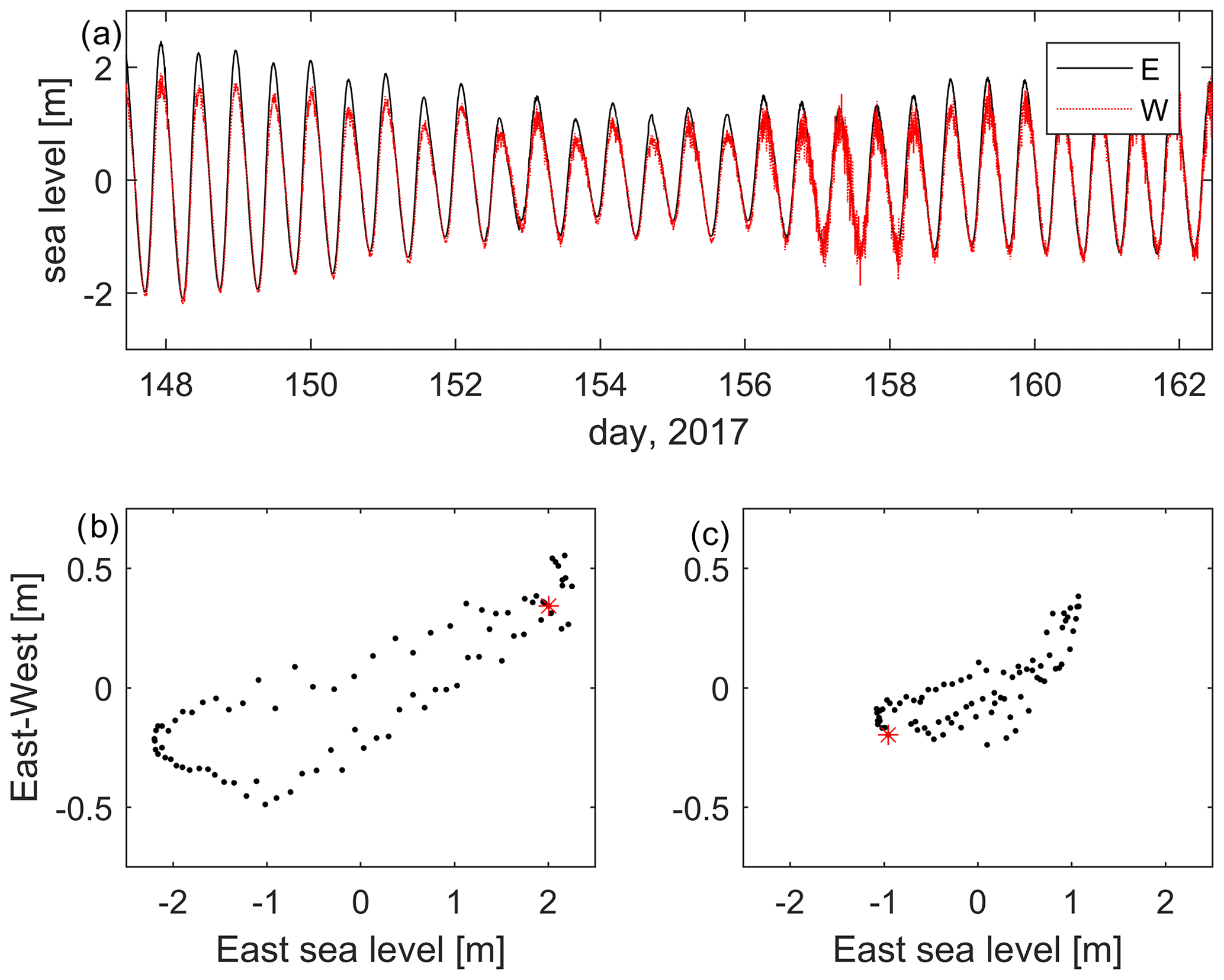
Figure 2(a) Part of the East (black) and West (red) data series for the in situ data from Deployment 1, covering one spring–neap cycle (arbitrary data). (b, c) Plots of the East–West elevation difference vs. the elevation at East for springs (b, day 147) and neaps (c, day 154). The red stars show the data point for 00:00 on the day. The progression is clockwise.
We do not have access to any current measurements from the region, but the tidal stream is known to reach up to 4 m s−1 in the sound (Colin Evans, personal communication, 25 May 2017, and Admiralty, 2017). There is also a simple interpretation of the differences in level across the island from East to West, which indirectly gives approximate values for the wider field of current speeds, which we term (but only in a local sense) the “far-field” currents. If we ignore any other effects, the pressure head across the island is given solely by the loss of kinetic energy due to the island blocking the flow (e.g. Stigebrandt, 1980). The same approach applies for wind forces on an impermeable fence or wall, and the sea level difference, Δh, between East and West is then given by the Bernoulli equation as
Here, v is the far-field tidal current speed and g the gravitational acceleration. Then we may indirectly compute the far-field tidal currents from the difference in levels across from East to West as the tide approaches the island (see Fig. 1 for the direction of the oncoming tide). Figure 3a and b (red curves) show the currents are computed for Day 147 (spring tides) and Day 154 (neap tides) with the speed shown in metres per second. The black curves are the measured sea levels at East. The computed far-field currents have a maximum over 3 m s−1 at springs and around 2 m s−1 at neaps, similar to local estimates (Colin Evans, personal communication, 25 May 2017). The noise in the level differences, which appears as noise in the currents (i.e. the red curves), may be an indication of turbulence and eddies discussed further below.
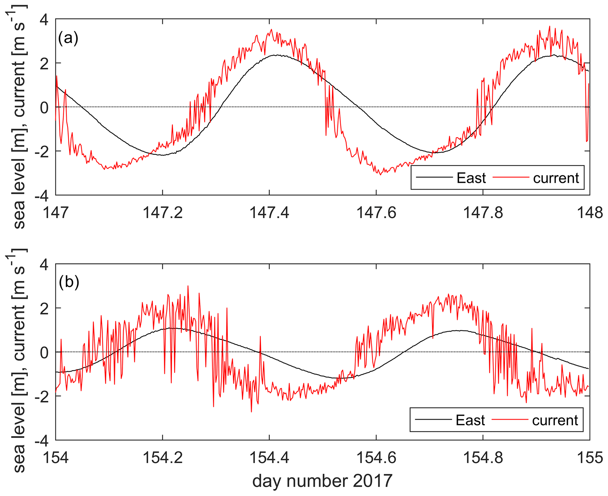
Figure 3(a) Computed current speeds for spring tides on Day 147 (27 May 2017) in metres per second (red) compared with the total sea levels at East (in metres, black). The computed current curve is noisy because the differences (E–W) are small. The phase relationship between currents is close to a progressive wave but with the current maximum to the northwest slightly in advance of the tidal high water. (b) As in (a) but for neap tides on Day 154 (4 June 2017).
Along the island the differences between Southwest and North are only a few millimetres for M2, within the confidence limits on the analyses. This curvature of the streamlines as the flow is squeezed through Bardsey Sound and swings up around the peninsula leads to the enhanced generation of non-linear higher tidal harmonics due to curvature on the reversing tidal stream curves (Pugh and Woodworth, 2014). This contributes to the large M4 amplitudes around the island and headland (Table 2).
Table 2Results of the tidal (TASK) harmonic analyses. “H” is amplitude (in m), and the phases “G” (degrees relative to Greenwich) are given in italics. The TPXO9 data was interpolated to the TG locations and the resulting data given to 0.01 m. The in situ RBR data results are given to 0.001 m and 1.0∘. However, for regional comparisons we assume confidence ranges of 1 % for amplitudes and 1.0∘ for phases. RBR constituents are adjusted for nodal and seasonal variations. Amplitudes are given to three decimal places as appropriate for the uncertainties in the RBR data, whereas the timing of constituent phases is probably better than 0.5∘ (1 min in time for M2).

3.2 Comparison with TPXO9 data
We turn now to a comparison of the tidal analysis data for M2 from the two sources (see Table 2 for details). When the TPXO9 M2 data, which have no Bardsey Island representation, are interpolated linearly to the TG positions, the result is only a 0.02 m and 0.7∘ amplitude and phase difference for the Deployment 1 locations. Compared to the 0.19 m amplitude difference and 6.5∘ phase difference in the TG data, it is clear that there is a substantial deficiency in the TPXO9 model in representing the role of the island due to its limited resolution. These results are supported by the Deployment 2 measurements (Table 2). Deployment 3 saw an extended and different approach to the data collection. We revisited East but also deployed two gauges on the Llŷn peninsula on the approach to the island (South Mainland), and north of it (North Mainland). At South Mainland, TPXO9 again underestimates the tidal amplitude by more than 10 %. At North Mainland, some 5 km north of Bardsey, and just north of the sound, however, the TG and TPXO9 amplitudes are within 1 cm of each other. This again shows the effect Bardsey and local topography have on the tidal amplitudes in the region.
As a representation of the shallow-water tidal harmonics, the TPXO9 M4 amplitude agrees well with the TG data at North (0.12 and 0.11 m, respectively) but overestimates the amplitude at North Mainland (0.07 m in the TG data and 0.12 m from TPXO; see Table 2). Because higher harmonics are generated locally by the tidal flow itself, this again shows the effect of the island on the tidal stream; the M4 amplitude is halved along Bardsey Sound in the TG data, whereas TPXO9 overestimates it and shows only minor variability. The overestimate in TPXO9 can lead to the tidal energetics being biased high in the region if they are based on the that data alone.
This is illustrated in the TPXO9 spring and neap flood currents in Fig. 4a–b, and the magnitude of the current in the sound in Fig. 4c. These currents are weaker than the far-field estimate using Eq. (1). For spring tides, TPXO9 shows a current of up to 1.5 m s−1 in the sound and 2.5 m s−1 in the far field, whereas the TG data and Eq. (1) comes out at 3.7 m s−1 from Eq. (1) for the spring tide far field (cf. Figs. 3 and 4). For neaps the corresponding values are 0.6 m s−1 in the sound and 1.5 m s−1 in the far field from TPXO9 and 3.0 m s−1 from the TG data and Eq. (1). The local sea-going experts (Colin Evans, personal communication, 25 May 2017) and the Admiralty chart for the sound (Admiralty, 2017) state a current speed of up 4 m s−1, and thus TPXO9 underestimates the currents in the strait by a factor ∼2.5, whereas the observations, even under the assumptions behind Eq. (1), get within 10 %. One can argue that the sea-level difference along the strait will lead to an acceleration into the strait as well (see, e.g. Stigebrandt, 1980), that could be added to the far-field current. However, frictional effects will come into play and a large part of the along-strait sea level difference will be needed to overcome friction and form drag (Stigebrandt, 1980). In fact, of the 0.32 m GA sea level difference between South Mainland and North Mainland (see Table 1), only 0.006 m is needed to accelerate the spring flow from 3.66 to 4 m s−1 in Eq. (1). That means that almost the entire sea level difference along the strait is due to energy losses.
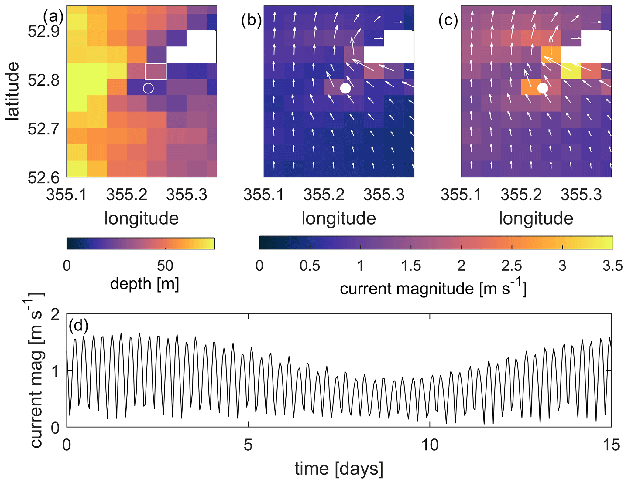
Figure 4(a) The depth from the TPXO9 database covering Bardsey Sound (marked with a white open circle). The rectangle northwest of the island shows the grid cell that the data in (d) were extracted from. (a–b) The current magnitude (colour) and vectors at neap (a) and spring (b) flood tides from TPXO9. These are computed from the M2 and S2 constituents only. The white circle shows the location of Bardsey; note that it is not resolved in the TPXO9 data and has been added for visual purposes only. (d) The magnitude of the tidal current during a spring–neap cycle in the sound (i.e. at the cell marked with a rectangle in (a) using the M2, S2, and M4 constituents in the TPXO9 data. Note that we chose to show data from the centre of the sound because that is where the computations using Eq. (1) are valid.
3.3 Dissipation
The dissipation in a tidal stream can also be computed from ε = ρCd|u|3, where Cd ∼ 0.0025 is a drag coefficient (Taylor, 1920) and ρ=1020 kg m−3 is a reference density. The peak dissipation using the computed GA current data from Eq. (1) and shown in Fig. 3 gives 777 MW for springs and 426 MW for neaps, assuming the sound is 3.1 km wide and 2.2 km long. This is 0.2 %–0.4 % of the 180 GW of M2 dissipation on the European shelf (see Egbert and Ray, 2000) and is a reasonable estimate for such an energetic region. Note that this method is independent of the phases between the locations and does not depend on the phases between the amplitudes and currents. If we instead use the TPXO9 current speed in the strait, the GA spring dissipation comes out as 53 MW (using u=1.5 m s−1), and the M2 dissipation (using a current speed of 1.2 m s−1) comes out as 28 MW. This is an underestimate of a factor 14 for the GA spring tide compared to the computation from the TG data, which again highlights the importance of resolving small-scale topography in local tidal energy estimates and the use of direct observations in coastal areas to constrain any modelling effort. This dissipation here is only a small fraction of the European Shelf and coastline, but it is a very energetic area. Although the Bardsey tides are unusually energetic, underestimated local coastal energy dissipation may be substantial in the TPXO9 (and similar) data and numerical models.
3.4 Caveat emptor!
We have shown above that the tidal elevations are underestimated in the TPXO9 data and that the current magnitude is most likely underestimated as well, and thus our computations of the energetics and non-dimensional numbers are conservative. The two extremes in tidal current magnitude in Bardsey Sound can be taken to be the neap tide speed from TPXO9 and the GA speed computed using TG data and TPXO9 combined. We thus have 0.9 m s−1 (neaps from TPXO9, not discussed above) as the lower range and 4 m s−1 (computed GA) as the upper estimate.
Even using the much-underestimated current speeds from the TPXO data, the indications are that there would be no stratification locally. The Simpson–Hunter parameter is for Bardsey Sound (Simpson and Hunter, 1974). This means that the area is vertically mixed due to the tides alone. The eddies shed from the island will add more energy to this, further breaking down any potential stratification from freshwater additions (the Simpson–Hunter parameter is based on heat fluxes only) and act to redistribute sediment. The associated Reynolds number for the island, , then comes out at approximately 10 for the neap flow or approximately 40 for the astronomic tidal current (using D=1000 m as the width and ν=100 m2 s−1 as the eddy viscosity). This implies laminar separation into two steady vortices downstream of the island at peak flows, and the vortices can be expected to appear on both ebb and flood flows (Edwards et al., 2004; Wolanski et al., 1984). There may not be any vortex shedding during neap flows, however, because Re∼10.
The Strouhal number is typically about 0.2 for the Re numbers found here (Wolanski et al., 1984), giving and an associated vortex-shedding period of 3–17 h (L=1500 m is the length of the island). This means that fully developed eddies can be generated at the higher flow rates because our tidal period (12.4 h) is longer than the vortex-shedding period by a few hours. However, at neap flows there is no time to develop a fully separated vortex within the time frame of a tidal cycle.
This conclusion is supported by satellite images from Landsat 8 (Fig. 5), which show a very different picture between neaps (Fig. 5a) and springs (Fig. 5b). At spring tides, there are two clear wakes behind the tips of the island (marked with magenta arrows), whereas at neaps (Fig. 5a) there is only a more diffuse image in Bardsey Sound and no signal of a wake behind the south tip of the island.
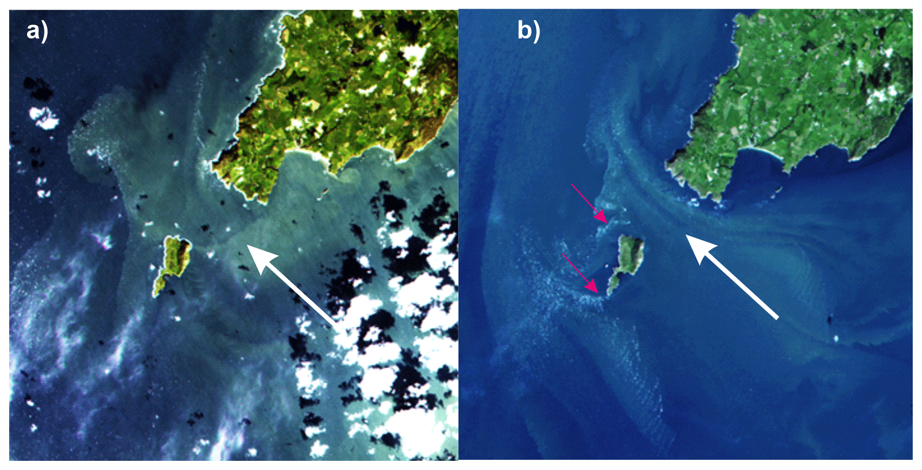
Figure 5Landsat 8 images from 5 October 2017 (a) and 13 September 2018 (b). The tidal phases are halfway through the tidal cycle on the neap flood in (a) and just after spring high tide in (b). The white dot north of the island in (b) is an exposed rock generating a second wake. See https://landsat.gsfc.nasa.gov/data/ (last access: 2 November 2020) for data availability.
This brief account was triggered by an interest in detailed mapping of tides in a reversing tidal stream. The results highlight the effect small coastal islands can have on tides in energetic settings, and they highlight the limitations of altimetry-constrained models near coastlines where the bathymetry used in the model is unresolved. Even though TPXO9, which is used here, is constrained by a series of tide gauges in the Irish Sea, including north and south of Bardsey, the island is some 60 km from the nearest long-term tide gauge (at Holyhead, to the north of Bardsey). Consequently, the tidal amplitudes in the database are not representative of the observed amplitudes near the island, and the currents are underestimated by a factor close to 2.5 for the GA tide. This underestimate also means that wake effects may be underestimated if one relies solely on altimetry-constrained models (or coarse resolution numerical models) unable to resolve islands, with consequences for navigation, renewable energy installations, and sediment dynamics.
Future satellite missions may be able to resolve small islands like Bardsey, and improved methods will allow for better detection of the coastlines. In order to obtain tidal currents, however, one still has to assimilate the altimetry data into a numerical model, and it will probably be some time before we can simulate global ocean tides at a resolution good enough to resolve an island like Bardsey.
The results do have wider implications for, among others, the renewable industry, because we show that local observations are necessary in regions of complex geometry to ensure the energy resource is determined accurately. Using only TPXO9 data, the dissipation – an indicator of the renewable resource – underestimates the astronomic potential by a factor up to 14 of the real resource. There is also the possibility that wake effects behind the island would be neglected without proper surveys, leading to an erroneous energy estimate. The results also highlight that concurrent sea level and current measurements are needed to fully explore the dynamics and quantify, e.g. further pressure effects of the island on the tidal stream. Consequently, we argue that in any near-coastal investigation of detailed tidal dynamics, the coastal topography must be explicitly resolved, and any modelling effort should be constrained to fit local observations of the tidal dynamics.
The data is available from the Open Science Framework (https://osf.io/kvgur/?view_only=ff2d8bd12a61493aa1dfa9011ecdde81, last access: 4 June 2020, Green, 2020).
JAMG wrote the manuscript and did the computations. DTP did the measurements, processed the TG data, and assisted with the writing.
The authors declare that they have no conflict of interest.
This article is part of the special issue “Developments in the science and history of tides (OS/ACP/HGSS/NPG/SE inter-journal SI)”. It is not associated with a conference.
Instrument deployments and recovery were planned and executed with the assistance of the Bardsey ferry operator, Colin Evans, and by Ernest Evans, a local lobster fisherman and expert on Bardsey tidal conditions. The Deployment 1 observations were partly funded by the Crown Estate. The Landsat data were processed by Madjid Hadjal and David McKee at University of Strathclyde, and constructive comments provided by Phil Woodworth and two anonymous reviewers improved the manuscript.
This paper was edited by Joanne Williams and reviewed by two anonymous referees.
Admiralty: Cardigan Bay Northern Part, Chart no. 1971, UK Hydrographic Office, Taunton , 2017.
Bills, B. G. and Ray, R. D.: Lunar orbital evolution: A synthesis of recent results, Geophys. Res. Lett., 26, 3045–3048, https://doi.org/10.1029/1999GL008348, 1999.
Dong, C., McWilliams, J. C., and Shchepetkin, A. F.: Island Wakes in Deep Water, J. Phys. Oceanogr., 37, 962–981, https://doi.org/10.1175/jpo3047.1, 2007.
Edwards, K. A., MacCready, P., Moum, J. N., Pawlak, G., Klymak, J. M., and Perlin, A.: Form Drag and Mixing Due to Tidal Flow past a Sharp Point, J. Phys. Oceanogr., 34, 1297–1312, https://doi.org/10.1175/1520-0485(2004)034<1297:fdamdt>2.0.co;2, 2004.
Egbert, G. D. and Erofeeva, S. Y.: Efficient inverse Modeling of barotropic ocean tides, J. Atmos. Ocean. Tech., 19, 183–204, 2002.
Egbert, G. D. and Ray, R. D.: Significant dissipation of tidal energy in the deep ocean inferred from satellite altimeter data, Nature, 405, 775–778, https://doi.org/10.1038/35015531, 2000.
Egbert, G. D. and Ray, R. D.: Estimates of M2 tidal energy dissipation from Topex/Poseidon altimeter data, J. Geophys. Res., 106, 22475–22502, 2001.
Green, J. A. M.: Bardsey – an island in a strong tidal stream, available at: https://osf.io/kvgur/?view_only=ff2d8bd12a61493aa1dfa9011ecdde81, last access: 4 June 2020.
Jakobsson, M., Mayer, L. A., Bringensparr, C., Castro, C. F., Mohammad, R., Johnson, P., Ketter, T., Accettella, D., Amblas, D., An, L., Arndt, J. E., Canals, M., Casamor, J. L., Chauché, N., Coakley, B., Danielson, S., Demarte, M., Dickson, M. L., Dorschel, B., Dowdeswell, J. A., Dreutter, S., Fremand, A. C., Gallant, D., Hall, J. K., Hehemann, L., Hodnesdal, H., Hong, J., Ivaldi, R., Kane, E., Klaucke, I., Krawczyk, D. W., Kristoffersen, Y., Kuipers, B. R., Millan, R., Masetti, G., Morlighem, M., Noormets, R., Prescott, M. M., Rebesco, M., Rignot, E., Semiletov, I., Tate, A. J., Travaglini, P., Velicogna, I., Weatherall, P., Weinrebe, W., Willis, J. K., Wood, M., Zarayskaya, Y., Zhang, T., Zimmermann, M., and Zinglersen, K. B.: The International Bathymetric Chart of the Arctic Ocean Version 4.0, Sci. Data, 7, 176, https://doi.org/10.1038/s41597-020-0520-9, 2020.
Kundu, P. K. and Cohen, I. M.: Fluid Mechanics, 2nd Edn., Academic Press, San Diego, 2002.
Magaldi, M. G., Özgökmen, T. M., Griffa, A., Chassignet, E. P., Iskandarani, M., and Peters, H.: Turbulent flow regimes behind a coastal cape in a stratified and rotating environment, Ocean Model., 25, 65–82, https://doi.org/10.1016/J.OCEMOD.2008.06.006, 2008.
McCabe, R. M., MacCready, P., and Pawlak, G.: Form drag due to flow separation at a headland, J. Phys. Oceanogr., 36, 2136–2152, https://doi.org/10.1175/JPO2966.1, 2006.
NOC: Tidal Analysis Software Kit, available at: https://www.psmsl.org/train_and_info/software/task2k.php (last access: 2 November 2020), 2020.
Piccioni, G., Dettmering, D., Passaro, M., Schwatke, C., Bosch, W., and Seitz, F.: Coastal Improvements for Tide Models: The Impact of ALES Retracker, Remote Sens., 10, 700, https://doi.org/10.3390/rs10050700, 2018.
Pugh, D. and Woodworth, P.: Sea-Level Science, Cambridge University Press, Cambridge, 2014.
Simpson, J. H. and Hunter, J. R.: Fronts in the Irish Sea, Nature, 250, 404–406, https://doi.org/10.1038/250404a0, 1974.
Stammer, D., Ray, R. D., Andersen, O. B., Arbic, B. K., Bosch, W., Carrère, L., Cheng, Y., Chinn, D. S., Dushaw, B. D., Egbert, G. D., Erofeeva, S. Y., Fok, H. S., Green, J. A. M., Griffiths, S., King, M. A., Lapin, V., Lemoine, F. G., Luthcke, S. B., Lyard, F., Morison, J., Müller, M., Padman, L., Richman, J. G., Shriver, J. F., Shum, C. K., Taguchi, E., and Yi, Y.: Accuracy assessment of global barotropic ocean tide models, Rev. Geophys., 52, 243–282, https://doi.org/10.1002/2014RG000450, 2014.
Stigebrandt, A.: Some aspects of tidal interaction with fjord constrictions, Estuar. Coast. Mar. Sci., 11, 151–166, 1980.
Taylor, G. I.: Tidal friction in the Irish Sea, Proc. R. Soc. Lon. Ser.-A, 96, 1–33, 1920.
Warner, S. J. and MacCready, P.: The dynamics of pressure and form drag on a sloping headland: Internal waves versus eddies, J. Geophys. Res., 119, 1554–1571, https://doi.org/10.1002/2013JC009757, 2014.
Wolanski, E., Imberger, J., and Heron, M. L.: Island wakes in shallow coastal waters, J. Geophys. Res., 89, 10553, https://doi.org/10.1029/jc089ic06p10553, 1984.
Woodworth, P. L., Shaw, S. M., and Blackman, D. L.: Secular trends in mean tidal range around the British Isles and along the adjacent European coastline, Geophys. J. Int., 105, 593–609, 1991.