the Creative Commons Attribution 4.0 License.
the Creative Commons Attribution 4.0 License.
 | 21 Jan 2020
Quantifying the contribution of shipping NOx emissions to the marine nitrogen inventory – a case study for the western Baltic Sea
Matthias Karl
Hagen Radtke
Volker Matthias
René Friedland
Thomas Neumann
The western Baltic Sea is impacted by various anthropogenic activities and stressed by high riverine and atmospheric nutrient loads. Atmospheric deposition accounts for up to a third of the nitrogen input into the Baltic Sea and contributes to eutrophication. Amongst other emission sources, the shipping sector is a relevant contributor to the atmospheric concentrations of nitrogen oxides (NOX) in marine regions. Thus, it also contributes to atmospheric deposition of bioavailable oxidized nitrogen into the Baltic Sea. In this study, the contribution of shipping emissions to the nitrogen budget in the western Baltic Sea is evaluated with the coupled three-dimensional physical biogeochemical model MOM–ERGOM (Modular Ocean Model–Ecological ReGional Ocean Model) in order to assess the relevance of shipping emissions for eutrophication. The atmospheric input of bioavailable nitrogen impacts eutrophication differently depending on the time and place of input. The shipping sector contributes up to 5 % to the total nitrogen concentrations in the water. The impact of shipping-related nitrogen is highest in the offshore regions distant from the coast in early summer, but its contribution is considerably reduced during blooms of cyanobacteria in late summer because the cyanobacteria fix molecular nitrogen. Although absolute shipping-related total nitrogen concentrations are high in some coastal regions, the relative contribution of the shipping sector is low in the vicinity of the coast because of high riverine nutrient loads.
- Article
(7312 KB) - Full-text XML
-
Supplement
(2224 KB) - BibTeX
- EndNote


The ecosystem of the Baltic Sea is exposed to anthropogenic pressures (Andersen et al., 2015; Korpinen et al., 2012; Svendsen et al., 2015). One major pressure is the high input of nutrients, i.e., bioavailable nitrogen and phosphorus compounds, leading to eutrophication (Svendsen et al., 2015). The eutrophication status has improved over the past decades (Andersen et al., 2017; Svendsen et al., 2015; Gustafsson et al., 2012). However, a Good Environmental Status (GES) has not been restored yet (e.g., HELCOM, 2009). Therefore, the descriptor 5 of the Marine Strategy Framework Directive (MSFD; EU-2008/56/EC, 2008) and the Baltic Sea Action Plan (BSAP) still focus on eutrophication (HELCOM, 2007).
Riverine nutrient loads have been evaluated in detail in the past decades (Sutton et al., 2011; Nausch et al., 2017; Stålnacke et al., 1999; HELCOM, 2013a; Svendsen et al., 2015). They approximately account for 2∕3 to 3∕4 of the bioavailable nitrogen input (HELCOM, 2013a, b). In addition, atmospheric deposition accounts for 1∕4 to 1∕3 of the total loads. Therefore, atmospheric nitrogen deposition is not negligible in the context of eutrophication (Simpson, 2011; HELCOM, 2005; Svendsen et al., 2015).
Atmospheric nitrogen deposition is higher above land than above water because a higher surface roughness leads to a higher dry deposition velocity (Seinfeld and Pandis, 2016, Chap. 19). Nevertheless, coastal waters are considerably impacted by atmospheric nitrogen deposition: the largest atmospheric emission sources of oxidized and reduced nitrogen compounds are located on land (CEIP, 2018), and coastal waters are closer to these sources than open ocean waters. Additionally, some gaseous nitrogen compounds condense on coarse sea salt particles, which have a short atmospheric residence time and hence deposit faster into the ocean (Paerl et al., 2002; Neumann et al., 2016). The western Baltic Sea is a region where high amounts of bioavailable nitrogen compounds are anthropogenically emitted (HELCOM, 2013b). Therefore, relatively high impacts by atmospheric deposition can be expected in this region compared to other parts of the Baltic Sea, which is why we selected it as our area of interest.
The shipping sector is an important contributor to atmospheric nitrogen oxide (NOX) air pollution in Europe and also in the Baltic Sea region (Jonson et al., 2015; Aksoyoglu et al., 2016). Thus, it considerably contributes to nitrogen deposition, particularly at the open sea. Tsyro and Berge (1998) found that the shipping sector contributed 5 % to 10 % to the NOX deposition in the Baltic Sea in 1990. The shipping sector contributed approximately 6 % to the total nitrogen deposition in 2000 (HELCOM, 2005) and approximately 14 % to the oxidized nitrogen deposition in 2005 (Bartnicki and Fagerli, 2008). In 2010, approximately 13 500 and 9500 t a−1 of the nitrogen deposition into the Baltic Sea originated from Baltic Sea and North Sea shipping, respectively. The total atmospheric nitrogen deposition accounted for 218 600 t a−1 and the waterborne nitrogen input for 758 300 t a−1 (HELCOM, 2013b). A specific target for a reduction of the annual nitrogen deposition from shipping was set to 5735 t a−1 within the latest revision of the HELCOM Baltic Sea Action Plan (HELCOM, 2013c).
The North Sea and Baltic Sea will be declared nitrogen oxide emission control areas (NECAs) according to the International Convention for the Prevention of Pollution from Ships Annex VI from 2021 onwards. That means that oceangoing ships built after 2021 have to comply with Tier III emission thresholds when they enter the North Sea and Baltic Sea regions. These emission thresholds force emission reductions of nitrogen oxides (NOX) by 75 % to 80 % compared to the currently valid Tier I and Tier II thresholds. Hence, NOX emissions of individual ships are expected to decline from 2021 onwards. However, shipping traffic is also expected to increase in the Baltic Sea in the next decades, and cargo vessels have a lifetime of approximately 25 to 30 years (e.g., Buhaug et al., 2009; Matthias et al., 2016; Karl et al., 2019a; Smith et al., 2014; Danish EPA, 2012). Therefore, the expected reduction in overall shipping NOX emissions will be rather low in the next decade (e.g., Geels et al., 2012; Jonson et al., 2015; Hammingh et al., 2012).
Commonly, studies on atmospheric nitrogen deposition focus only on the input of bioavailable nitrogen but not on its processing in the Baltic Sea (EMEP, 2017; Bartnicki and Fagerli, 2008; Tsyro and Berge, 1998; HELCOM, 2005; Stipa et al., 2007; Bartnicki et al., 2011; Hongisto, 2014). However, the impact of one input source sector, i.e., shipping, on the marine biogeochemistry not only depends on its annual input but also on the residence times of nutrients in the system and on the location of their deposition sites. These residence times are governed by the location and time of the nutrient release as well as by the availability of other nutrients. Hence, the amount of shipping-related nitrogen deposition relative to other nitrogen inputs is not necessarily linearly related to its impact.
This led to our central research question: how high is the contribution of shipping-related nitrogen deposition to concentrations of total nitrogen (TN) and of individual nitrogen fractions in the western Baltic Sea? We approached this question by the means of a modeling study.
A coupled marine physical biogeochemical model was applied to simulate the western Baltic Sea combined with a tagging method previously applied to riverine inflow (Radtke et al., 2012) and saltwater inflow events (Neumann et al., 2017). Raudsepp et al. (2013) performed a similar study focusing on the impact of shipping-related nitrogen deposition on nitrogen fixation by cyanobacteria in the Gulf of Finland. Raudsepp et al. (2019) assessed shipping-related nutrient inputs – nitrogen and phosphorus from atmospheric deposition and direct discharge – into the Baltic Sea, focusing rather on the Gotland Basin. The authors traced the shipping contribution by calculating the difference between two simulations with and without shipping-related nitrogen deposition but did no tagging. Tagging of atmospheric nitrogen deposition has been done for the North Sea and the English Channel in several studies (e.g., Große et al., 2017; Los et al., 2014; Troost et al., 2013; Ménesguen et al., 2018; Dulière et al., 2017). The method has also been used to tag nitrogen compounds in atmospheric chemistry transport model simulations (e.g., Brandt et al., 2011; Geels et al., 2012; Wu et al., 2011).
The marine biogeochemical modeling was done with MOM–ERGOM (Modular Ocean Model–Ecological ReGional Ocean Model). The atmospheric nitrogen deposition was calculated by the Community Multiscale Air Quality (CMAQ) modeling system, which is an atmospheric chemistry transport model. The model systems were not coupled online. First, simulations were performed with CMAQ. Then, simulations were performed with MOM–ERGOM using nitrogen deposition from CMAQ as forcing. Both model simulations were forced by meteorological data from the coastDat2 and coastDat3 datasets calculated by COSMO-CLM (Consortium for Small-scale Modeling–Climate Mode). Nitrogen from shipping-related atmospheric deposition was tagged in ERGOM and traced through the biogeochemical system. This procedure allowed for the identification of the shipping contribution to different nitrogen fractions. Shipping-related nitrogen deposition was available from the CMAQ simulations.
The MOM–ERGOM simulations with tagging of shipping-related nitrogen deposition were performed from 2006 to 2012. The model was previously spun up for several decades without tagging. The nitrogen deposition data were only available for the year 2012. Therefore, all seven simulated years were forced by the same nitrogen deposition data. The years 2006 to 2011 were only used for the model validation and are considered tagging spin-up. The year 2012 is used for the evaluation of the contribution of shipping-related nitrogen deposition.
2.1 Atmospheric modeling
The meteorological forcing data for the MOM–ERGOM simulations were taken from the coastDat2 dataset and were calculated by COSMO-CLM (Weisse et al., 2015; Geyer, 2014; Geyer et al., 2015; HZG, 2017) using version 4.8-clm-11 (Rockel et al., 2008; Geyer and Rockel, 2013) on a regular longitude–latitude grid of 0.22∘ × 0.22∘ horizontal resolution with a rotated pole at 170.0∘ W and 35.0∘ N, with spectral nudging applied to assimilate large-scale wind data.
The atmospheric biogeochemical forcing data for the MOM–ERGOM simulations was calculated by CMAQ. The CMAQ model is maintained and provided by the U.S. Environmental Protection Agency. For this study, we used CMAQ version 5.0.1 (Nolte et al., 2015; Foley et al., 2010; Appel et al., 2017) with the cb05tucl gas-phase chemistry mechanism (Sarwar et al., 2007; Whitten et al., 2010; Yarwood et al., 2005) and aero5 aerosol chemistry, which is based on ISORROPIA v1.7 (Fountoukis and Nenes, 2007; Sarwar et al., 2011). Atmospheric particles are represented by a three-moment scheme containing three size modes (Binkowski and Roselle, 2003). The dry deposition parameterization for particulate matter is an updated version of Binkowski and Shankar (1995), which is based on Slinn and Slinn (1980) and Pleim et al. (1984). The parameterization considers gravitational settling, aerodynamic resistance above the canopy, and surface resistance. The three modes and the three moments are deposited individually. Land-based emissions were aggregated with SMOKE for Europe (Sparse Matrix Operator Kernel Emissions; Bieser et al., 2011). Marine shipping emissions were calculated with STEAM (Ship Traffic Emission Assessment Model; Jalkanen et al., 2012) based on data from the automatic identification system (AIS). Via AIS modern ships broadcast their location, direction of travel, speed, IMO number (IMO: International Maritime Organization), and further information. Ships are considered to emit NOX but no reduced nitrogen. Sea salt emissions were calculated online (Gong, 2003; Kelly et al., 2010) without surf zone emissions (Neumann et al., 2016).
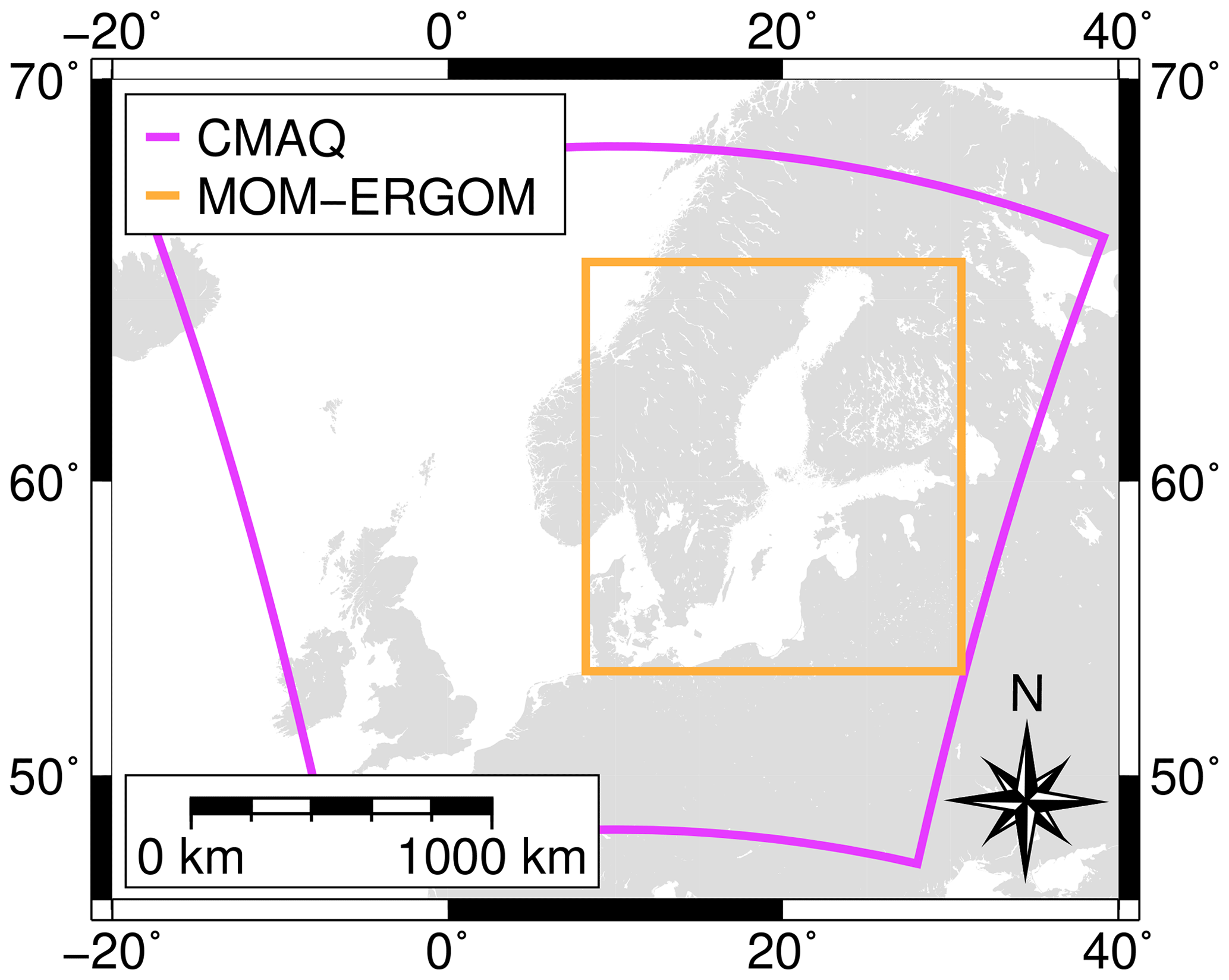
Figure 1Extent of the model domains of the atmospheric chemistry transport model (CMAQ) and of the marine biogeochemical model (MOM–ERGOM).
The CMAQ simulations were performed on two one-way nested model domains with increasing horizontal grid resolution (Fig. 1) and 30 vertical z layers each. The outer model domain (64×64 km2 grid resolution) covered Europe and northern Africa. The lateral boundary conditions were taken from the FMI APTA global reanalysis (Sofiev et al., 2018). The first nested model domain (16×16 km2 grid resolution) covered the North Sea and Baltic Sea regions. The latter data were used as atmospheric input data for the biogeochemical modeling experiments. The following CMAQ system variables were summed to obtain oxidized and reduced nitrogen deposition.
-
Oxidized nitrogen: NO, NO2, HNO3, N2O5, , NO3, HONO, PAN (peroxyacetyl nitrate), PNA (peroxynitric acid; only wet deposition)
-
Reduced nitrogen: NH3,
St-Laurent et al. (2017) considered the same CMAQ variables to calculate nitrogen deposition into the ocean but additionally estimated dissolved organic nitrogen (DON) deposition according to Zhang et al. (2012). Detailed DON deposition measurements were not available for the region of interest. Therefore, atmospheric deposition of DON was not considered in this study. Figure 2 shows the resulting annual mean nitrogen deposition in the western Baltic Sea region and the contribution from the shipping sector.
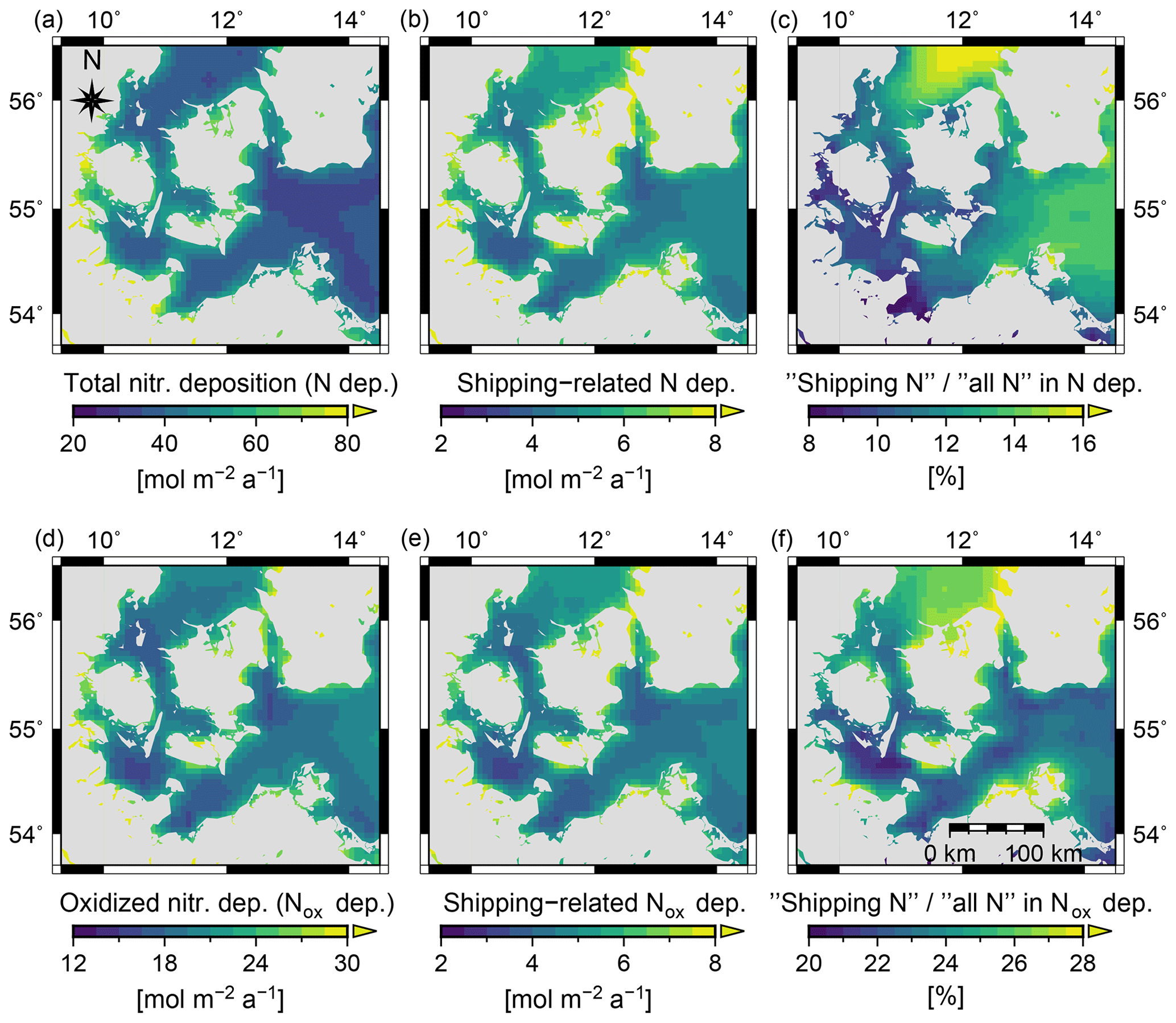
Figure 2Annual mean deposition of total nitrogen (TN, a–c) and oxidized nitrogen (NOX, d–f) calculated by the CMAQ model. The nitrogen deposition (nitrogen from all sources, a, d), the shipping-related nitrogen deposition (b, e), and the quotient between the two (c, f) are plotted.
Meteorological input data for the CMAQ simulations were modeled with COSMO-CLM version 5.00_clm8 with spectral nudging (Rockel et al., 2008) on a rotated grid of 0.11∘ spatial resolution. This dataset is available as the coastDat3 atmosphere dataset of the Helmholtz-Zentrum Geesthacht (http://www.coastdat.de/, 10 January 2020; HZG, 2017).
Karl et al. (2019a, b) describe the model setup in more detail and present a validation for the simulation results with respect to the atmospheric deposition. The wet deposition of oxidized and reduced nitrogen was systematically underestimated at Baltic Sea stations. The reported underestimation is consistent with results of Vivanco et al. (2017). Nitrogen deposition in CMAQ simulations with very similar forcing data in the same region but in different years was evaluated. The reason for the underestimation could not be fully resolved in Karl et al. (2019a). It is assumed that either NOX to HNO3 conversion is too slow, possibly because of ammonia background concentrations that are too low, or that the wet removal of and is too low. Modeled atmospheric concentrations of NOX did properly reproduce measurements at European Measurement and Evaluation Programme (EMEP) stations.
The nitrogen deposition dataset was bilinearly interpolated onto the MOM–ERGOM model grid resolution and supplied as daily mean values.
2.2 Marine modeling
The ocean physics were simulated with the Modular Ocean Model (MOM) version 5.1 (Griffies, 2004). The whole Baltic Sea was modeled with a horizontal resolution of 3 nmi × 3 nmi (nmi: nautical mile) and 134 vertical layers. Open boundary conditions were provided as climatological data in the Skagerrak, the connection to the North Sea. A dynamic ice model simulates ice cover (fraction of grid cell area), thickness, and extent. MOM has been used for several studies of the Baltic Sea and has been extensively validated (e.g., Neumann et al., 2015; Radtke et al., 2012; Schernewski et al., 2015).
The marine biogeochemical processes are simulated with the Ecological ReGional Ocean Model (ERGOM), which has been developed at the Leibniz Institute for Baltic Sea Research Warnemünde and is still under active development (Neumann, 2000; Neumann et al., 2002, 2015; Kuznetsov and Neumann, 2013; Radtke et al., 2013). It was coupled to MOM and shared the same model domain. The nitrogen deposition data were supplied in daily resolution. Riverine nutrient loads were taken from the Updated Fifth HELCOM Baltic Sea Pollution Load Compilation (HELCOM, 2015).
In the ERGOM version used, the biogeochemical system is represented by 31 state variables (“tracers”), 26 of which are in the water column and 5 in the surface sediment. Inorganic nutrients – i.e., nitrate (, ammonium (), and phosphate () – enter the system via river input, atmospheric deposition, and remineralization of organic matter. They are consumed by phytoplankton that are represented by large phytoplankton, small phytoplankton, and cyanobacteria. Large phytoplankton start growing at lower temperatures than small phytoplankton but process nutrients less efficiently, meaning that they run into nutrient limitation more quickly than small phytoplankton. The growth of cyanobacteria depends only on and molecular nitrogen (N2), which they fix to cover their nitrogen demand. Phytoplankton, including cyanobacteria, are grazed by zooplankton. Plankton respirate and die. Dead plankton become detritus that sinks to the sediment. The sediment is represented by a one-layer sediment including several relevant sediment processes such as phosphate release under anoxic conditions or denitrification. Nutrients may be retained in the sediment, deeply buried, or resuspended. All state variables, processes, and constants are listed in a detailed model documentation in the Supplement.
Shipping-related atmospheric nitrogen deposition was tagged by the method described by Ménesguen et al. (2006). It has been implemented in ERGOM and used in previous studies (e.g., Neumann, 2007; Radtke et al., 2012). All state variables containing nitrogen are duplicated: one variable containing all nitrogen in the particular compound and another variable containing only the shipping-related nitrogen. The first type of state variable is denoted as “all NAME” or “NAMEall”, whereas the latter type is denoted as “shipping NAME” or “NAMEship”. Process rates are calculated for the original state variables and are then linearly scaled according the NAMEship-to-NAMEall ratio of the educts (also written as NAMEship ∕ NAME).
Monthly mean concentrations of all state variables were written out in full spatial resolution. Basin mean concentrations were calculated from these data and are hence only available as monthly means. Daily mean concentrations were written out in full vertical resolution at the locations of measurement stations (see Sect. 2.5).
2.3 Study region
The western Baltic Sea was chosen as the study region. It is bordered by land in the south, west, and northeast. Danish islands like Zealand and Funen are located in the center of this region (Fig. 3).
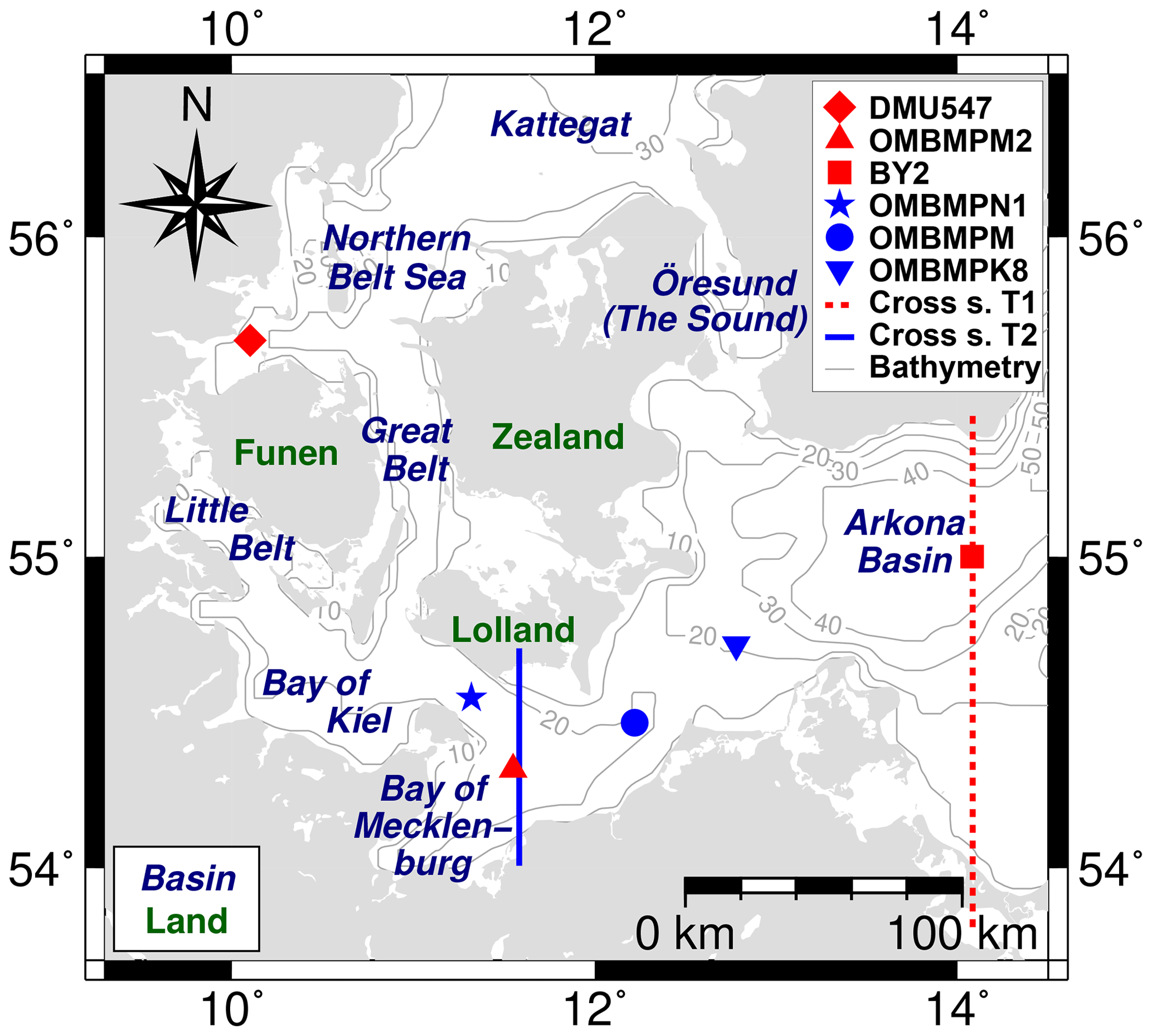
Figure 3Study region, measurement stations, cross sections for evaluation, and geographic locations mentioned in this publication. Basins of the Baltic Sea and of the Kattegat are printed in navy blue italic font. Islands and peninsulas are printed in green. Measurement stations are indicated by symbols and colors as defined in the legend (top right). Cross sections for model evaluation are indicated by red dotted (T1) and blue solid lines (T2). Red stations and lines are considered in this paper (top three stations in the legend) and blue stations and lines in the Supplement (items four to six in the legend). The solid gray lines with numbers attached are isolines of the bathymetry. The numbers give the depth in meters.
The land use south and west of the study region is dominated by agricultural activities, which lead to nutrient inputs into the Baltic Sea via rivers and the atmosphere. The population density is lower than along the southern North Sea but still high, inducing the input of various types of pollutants, i.e., organic pollutants, heavy metals, and plastic litter. The shipping traffic volume is high because a major European shipping route leads through this region connecting harbors in the Baltic Sea to the North Sea and more distant locations. Hence, the deposition of atmospheric shipping emissions and direct discharges of ships import pollutants and nutrients into the Baltic Sea.
The seawater of the Baltic Sea is brackish with a strong gradient in the salinity starting with 20 to 25 g kg−1 in the Kattegat to salinities below 2 g kg−1 in the Bothnian Bay and in the eastern parts of the Gulf of Finland. The region of interest is characterized by strong north–south ( in the north and in the Bay of Mecklenburg) and west–east gradients ( in the Bay of Kiel and in the Arkona Basin). These salinity gradients affect the phytoplankton species composition: cyanobacteria grow only in regions with salinities below (Wasmund, 1997).
The Baltic Sea surface water is well mixed in the upper 40 m by convection and wind-induced turbulence in winter (Feistel et al., 2008). No algal bloom develops as long as the water column is well mixed because algae are mixed too deep where they do not get sufficient sunlight. When the wind speeds decrease in spring, the water column becomes stratified by the development of a thermocline at 25 to 30 m of depth and the temperature in the surface water rises. Hence, the beginning of the algal bloom in spring strongly correlates with calmer weather and the emergence of stratification. First, diatoms begin to bloom in the nutrient-enriched surface waters in February to May (Neumann et al., 2002). Nutrient concentrations decrease and flagellates, which are more efficient in their nutrient uptake than diatoms, start blooming in April or May and reach their peak in July. The bloom declines when one of the required nutrients is depleted in summer. The biogeochemical system is nitrogen limited in most parts of the Baltic Sea, indicated by nitrogen-to-phosphorus (N:P) ratios below 16, which is the Redfield ratio (Feistel et al., 2008, Sect. 12.3, Table 12.3). Hence, excess phosphorus remains in the surface water after the diatoms and flagellates bloom. The N : P ratio in riverine nutrient loads is mostly larger than 16:1, indicating phosphorus limitation (Svendsen et al., 2015). However, the areas affected by river plumes and phosphorus limitation are rather small. Cyanobacteria bloom in late summer. They fix dissolved N2 and are hence not affected by depleted nitrate and ammonium. The algal bloom period ends in autumn when the stratification is broken up by autumn storms.
2.4 The year 2012
Only one year (2012) was considered to be analyzed with this study.
In 2012 there were no exceptionally strong Baltic Sea inflows from the North Sea, which might have affected salinity, temperatures, and physical parameters (Mohrholz, 2018a). The precipitation amount in northern Europe in 2012 was above the long-term average EMEP (2014, p. 49). Hence, the freshwater inputs were higher than in the previous years. The riverine nutrient loads were not exceptionally high compared to the long-term average. Further, Savchuk (2018) assessed the nutrient dynamics from 1970 to 2016 based on measurement data and concluded that 2012 was no exceptional year with respect to DIN (dissolved inorganic nitrogen), TN (total nitrogen), DIP (dissolved inorganic phosphorus), and TP (total phosphorus) in the water.
The nitrogen wet deposition in northern Europe in 2012 was above the average of the previous 10 years due to the increased precipitation (EMEP, 2014). The nitrogen dry deposition in northern Europe in 2012 was lower than in the previous 10 years (higher wet leads to lower dry deposition), but the total nitrogen deposition (dry + wet) was still higher. The NOX emissions in Europe in 2012 were lower than in the previous 10 years. While the deposition of oxidized nitrogen compounds in southern Europe was lower compared to previous years due to lower emissions, it slightly increased in northern Europe due to the higher wet deposition. The ammonia emissions are treated differently in SMOKE for Europe than in the EMEP emission model. Therefore, the information on reduced nitrogen deposition in EMEP (2014) is not applicable here. Unfortunately, the emissions by SMOKE for Europe were specifically created for the year 2012 and are not fully comparable to the previous SMOKE for Europe emissions created for other years.
Summarizing, the year 2012 was no exceptional year with respect to central nutrient dynamics. In the evaluation of EMEP model results, the total nitrogen deposition in northern Europe was slightly increased due to increased precipitation. However, this might not be the case in this study because nitrogen deposition in the CMAQ data was lower than in the EMEP data.
2.5 Validation and evaluation
The results of MOM–ERGOM simulations were validated against observational data at specific stations (see Table 1 and Figs. 3 and 4). Vertical profiles were measured at most stations. Measurements and model data for salinity, temperature, nitrate (), and phosphate () were averaged over the top 10 m and over the bottom 8 to 10 m for this purpose. The measurement data were taken and merged from two sources:
-
the measurement database of the Leibniz Institute for Baltic Sea Research (IOWDB; https://www.io-warnemuende.de/iowdb.html, last access: 10 January 2020) and
-
the HELCOM oceanographic measurement database hosted by the International Council for the Exploration of the Sea (ICES; http://ocean.ices.dk/helcom/Helcom.aspx, last access: 10 January 2020).
A statistical validation of the model results with measurement data is difficult because the number of observations is limited – far below one measurement per month at most stations. Therefore, 7 years of data were summarized on a monthly basis to a 1-year “climatology”. The climatological median and spread (10th to 90th percentiles) of the measurement and model data time series were then visually compared.
Table 1List of stations used for validation. The first three stations (DMU547, OMBMPM2, and BY2) are considered in the paper, whereas the last three stations are presented in the Supplement. See also Figs. 3 and 4 for maps containing the station locations.
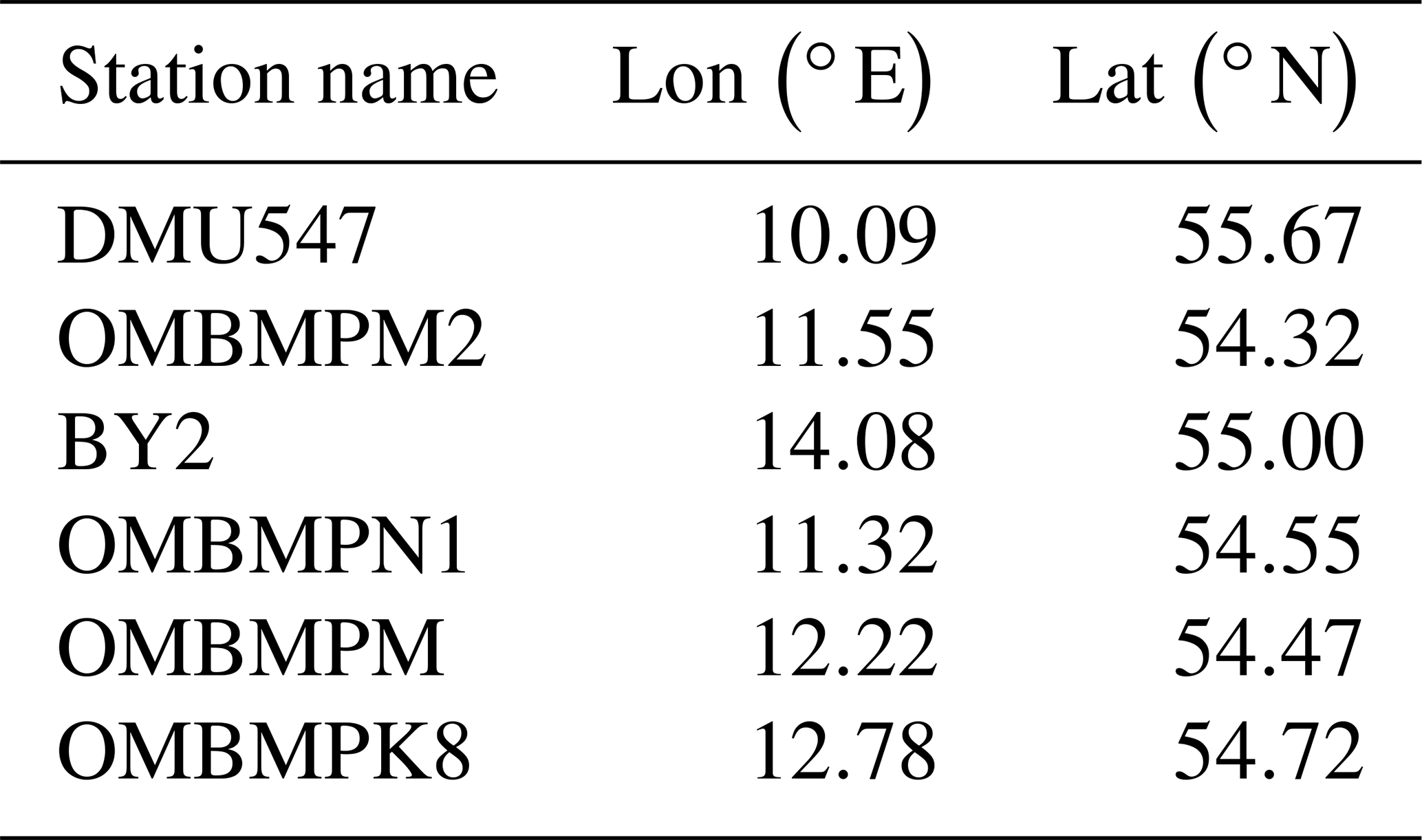
Three stations were chosen to be presented in the Results section. They represent different regimes in the considered region: two offshore stations in different basins (OMBMPM2 and BY2) and one station close to the shore (DMU547). Validation plots at three additional stations are presented in the Supplement and show a similar outcome.
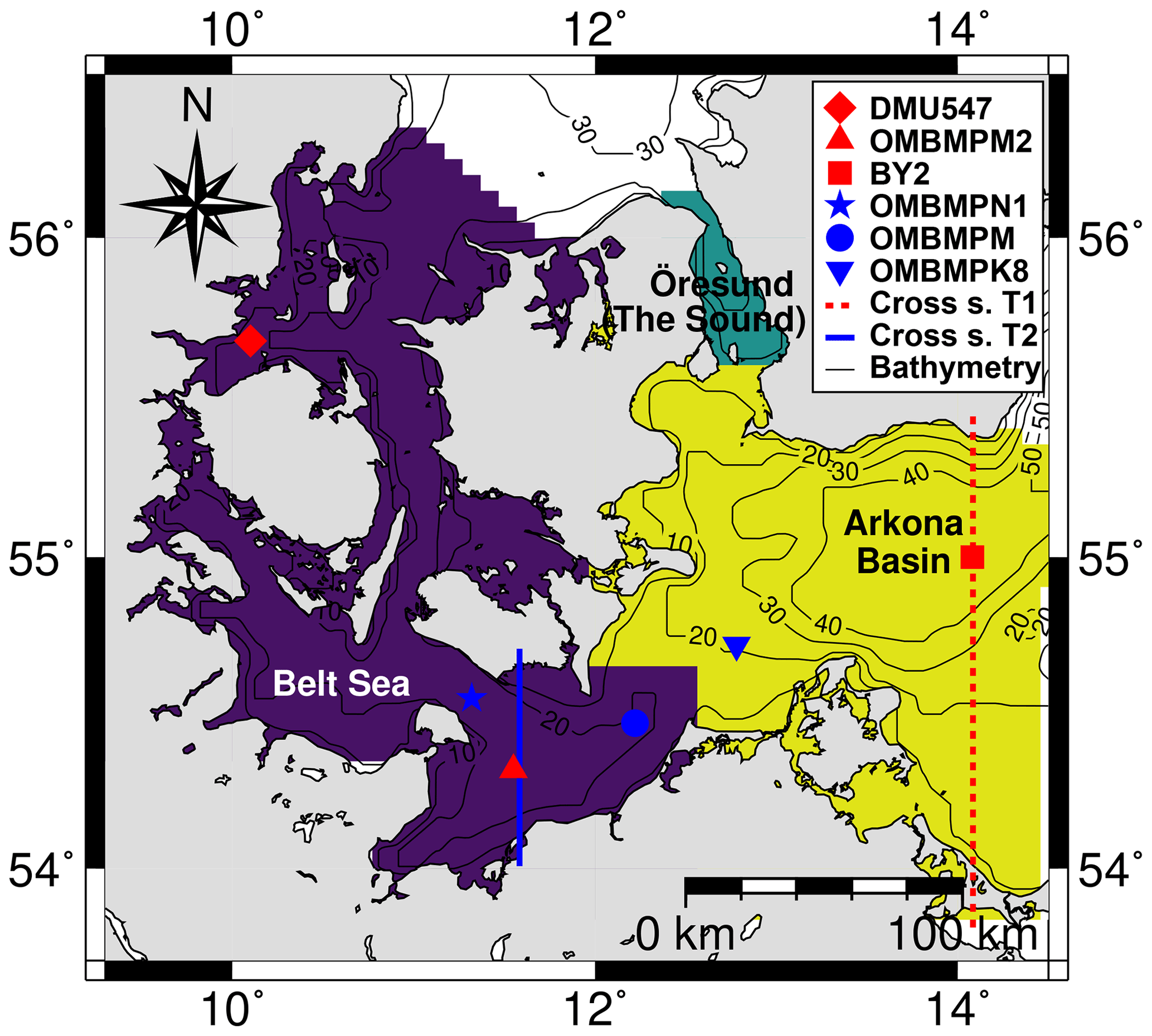
Figure 4Basins in the western Baltic Sea according to Omstedt et al. (2000) drawn in yellow (Belt Sea), green (Arkona Basin), and cyan (Öresund). Measurement stations are indicated by red and blue symbols. Cross sections for model evaluation are indicated by red dashed and blue solid lines. Red stations and lines are considered in this paper (top three stations in the legend) and blue stations and lines in the Supplement (items four to six in the legend). The dark thin lines with numbers attached are isolines of the bathymetry. The numbers give the depth in meters.
The atmospheric shipping contribution to the nitrogen budget was assessed on the basis of (a) the listed stations and (b) horizontal mean values per basin. Basin definitions by Omstedt et al. (2000) were used for this study (Fig. 4). The definitions of the basins are based on the bathymetry: e.g., the Belt Sea and the Arkona Basin are separated by the Darss Sill, which is located a bit northward of station OMBMPM. The Kattegat is not considered because the concentrations of tagged compounds might be impacted by the model's open boundary in the Skagerrak.
3.1 Validation
Figures 5 and 6 show climatological time series generated from model and measurement data for the years 2006 to 2012.

Figure 5Monthly climatological medians of observational (dots) and modeling data (solid lines) at the sea surface (top 10 m) from 2006 to 2012. Each row presents the data of one station ordered from west (top) to east (bottom). The station names and depth range are given on the left. Each column presents one state variable: salinity, temperature, nitrate, and phosphate (from left to right). Vertical lines through the dots and the shaded area around the solid line show the monthly variability represented by the 10th and 90th percentiles. The number of observational data points per month is given above the x axis of each plot. A similar figure showing data at the other three stations is provided in the Supplement.
Sea surface temperature is well reproduced by MOM at all stations, but sea surface salinity is overestimated at OMBMPM2 and BY2. This is a known issue and has been documented previously (e.g., Neumann and Schernewski, 2008). No measurements at the seafloor were available at DMU547. At the seafloor at OMBMPM2, the modeled salinity exceeds the measurements and the amplitude of the seasonal cycle of the modeled temperature seems to be too low. This might point to issues in the vertical transport in the Bay of Mecklenburg.
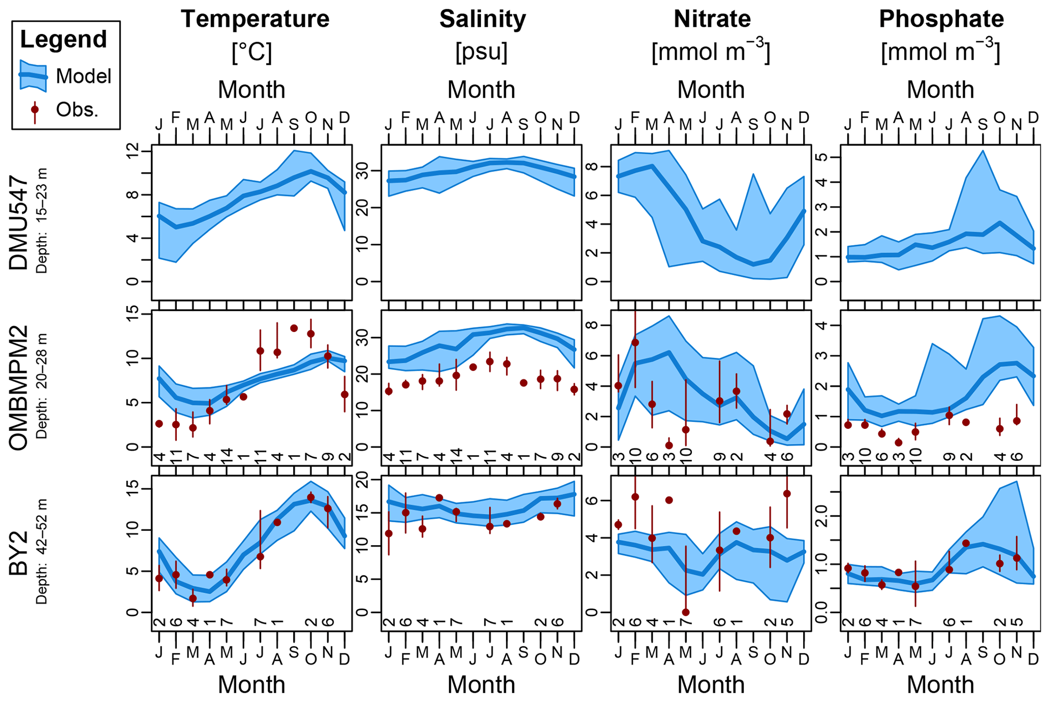
Figure 6Similar to Fig. 5 but for the bottom 8 to 10 m. The exact depth range is given on the left. A similar figure showing data at the other three stations is provided in the Supplement.
Modeled sea surface nitrate and phosphate concentrations agree well with the measurements, although phosphate concentrations are slightly underestimated. The seasonal pattern of modeled concentrations is realistic at all stations at the sea surface. At the seafloor, the annual cycle of nitrate does not seem to be captured by the model at OMBMPM2. Modeled nitrate concentrations increase in spring, but measurements show a decrease. Simulated salinity suggests that stratification is overestimated by the model, leading to a lower impact of surface processes on deeper water layers. This also causes the damped amplitude of the annual temperature cycle. At BY2, the annual cycle of nitrate and phosphate concentrations is reproduced by MOM–ERGOM, but the nitrate depletion in spring is underestimated.
3.2 Spatial pattern of shipping-related nitrogen
Figure 7 provides an overview of the spatial distribution of shipping nitrogen in total nitrogen (TNship). The TNall concentrations are high in the vicinity of major river estuaries, particularly close to the Oder River in the bottom right of the plotted domain and northward of Zealand, and have a strong horizontal gradient towards the open water.
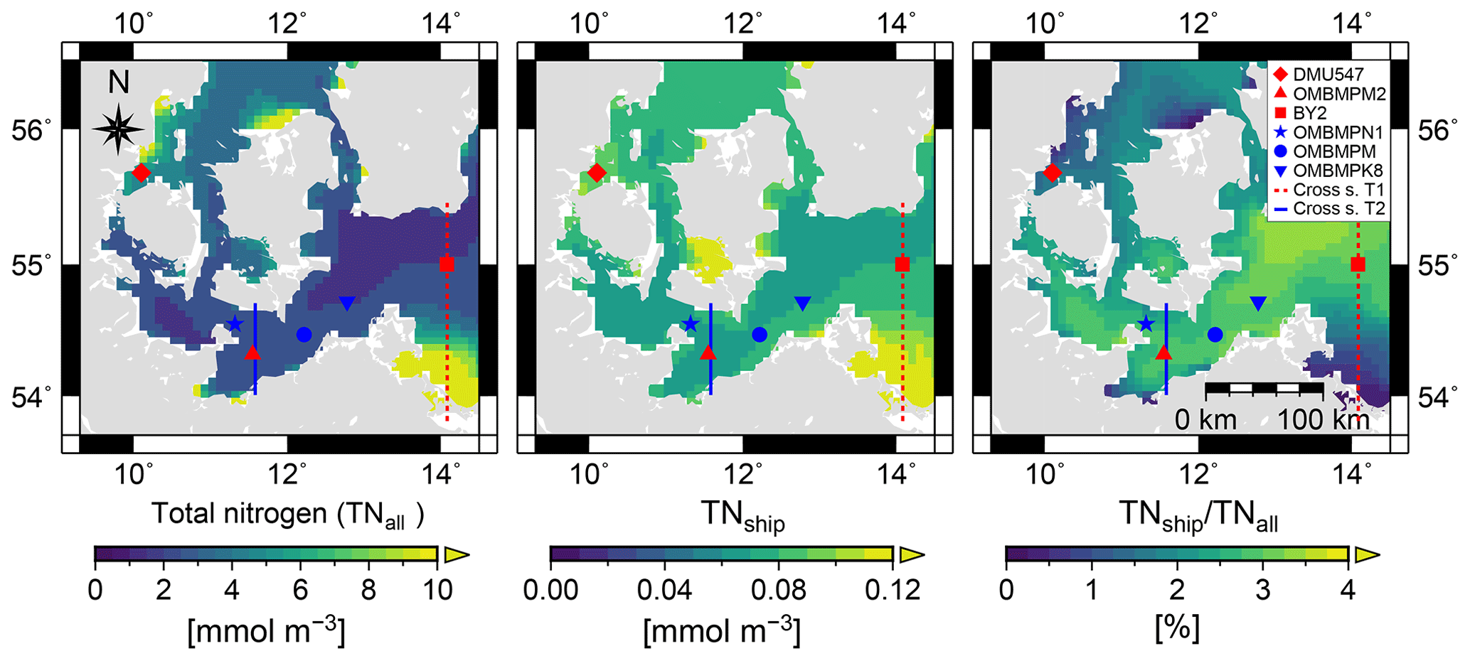
Figure 7Spatial pattern of the modeled total nitrogen concentration (TNall), the total nitrogen concentration with nitrogen from shipping-related atmospheric deposition (TNship), and the ratio of the two (TNship∕TNall). Modeled data for the year 2012 of the top 10 m are used. Measurement stations and cross sections used in other parts of the evaluation are included as symbols and lines, respectively.
The TNship concentrations are very high close to the Oder River estuary and between Zealand and Lolland. They are also slightly increased in the region around station DMU547. The spatial pattern is more homogeneous than that of the TNall concentrations, and it reveals considerably smaller spatial gradients. Shipping routes are not visible because NOX from shipping emissions does not necessarily deposit close to sources but might be transported over longer distances. A reason for this is the high atmospheric residence time of NOX. Possible reasons for the peaks along the shoreline are discussed in Sect. 4.
The contribution of shipping-related nitrogen to TN (TNship∕TNall) does not exceed 4 % on annual average. It is lowest in regions close to river estuaries (<1 %) and increases towards the open water.
3.3 Seasonal cycle of shipping-related nitrogen
The annual cycles of nitrogen compounds in the surface layer of three basins are plotted in Fig. 8.
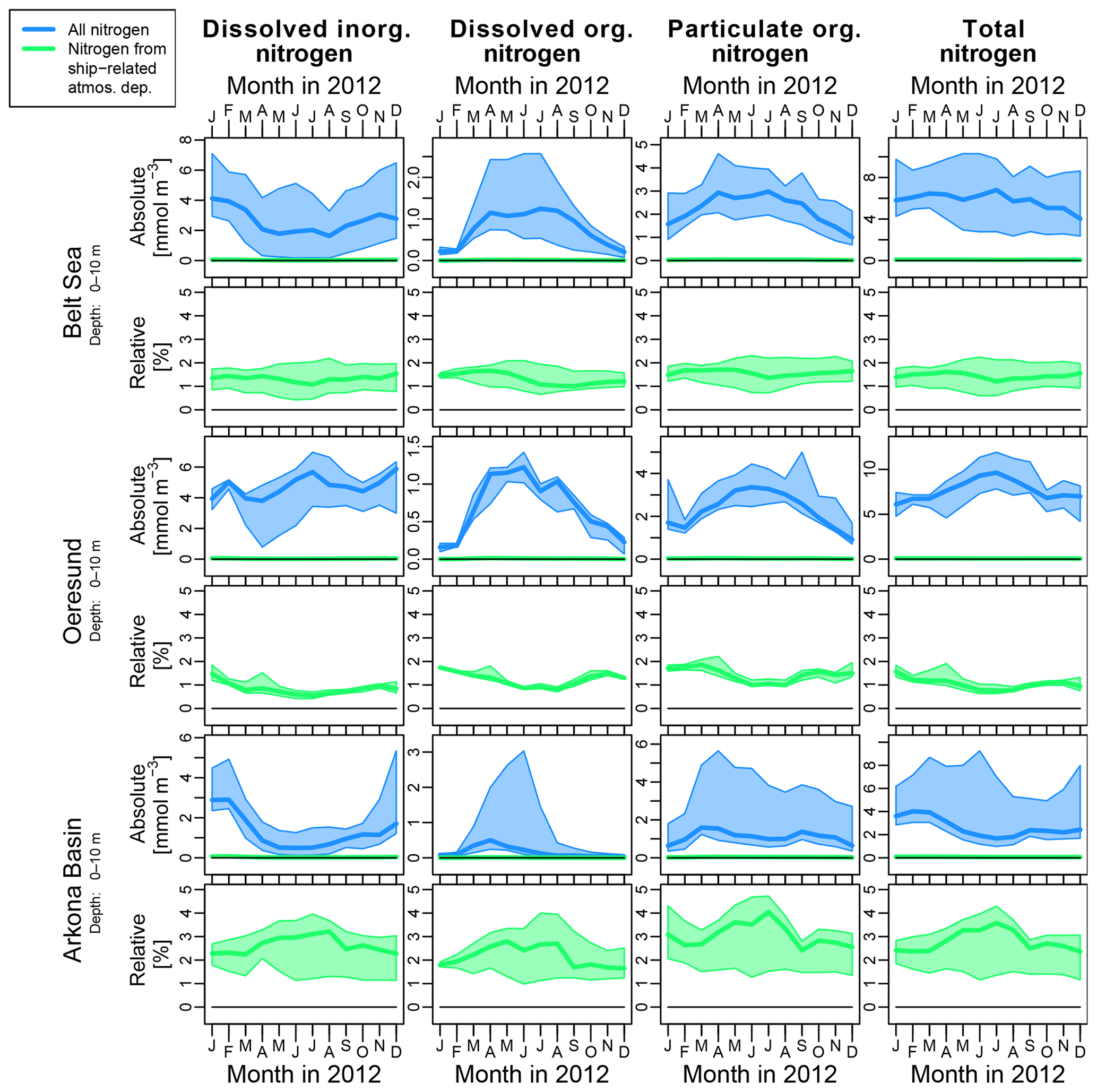
Figure 8Monthly concentrations of dissolved inorganic nitrogen (DIN), dissolved organic nitrogen (DON), particulate organic nitrogen (PON), and total nitrogen (TN), with all nitrogen (blue; darker color in grayscale) and shipping-related nitrogen (green; lighter color in grayscale) in the odd rows. The ratio between shipping-related and all nitrogen of the same compounds is in the even rows. Each pair of rows represents data for one of the basins: Belt Sea, Öresund, and Arkona Basin (top to bottom). The horizontal median as well as the 10th and 90th percentiles are plotted. The thick lines are the medians and the shaded area covers the interval between the 10th and 90th percentiles. The statistics were calculated from monthly and vertically (top 10 m) averaged concentrations. For the ratios, (first) the vertical and temporal averages, (second) the quotients, and (third) the median and percentiles were calculated.
The concentrations of dissolved inorganic nitrogen (DINall) in the Belt Sea and in the Arkona Basin decrease in spring, have their minimum in summer, and increase in autumn. This is an expected and typical system behavior: DIN accumulates in winter, is consumed by phytoplankton in the growth period, and is reimported into the surface layer from below by vertical mixing in autumn. Correspondingly, the concentrations of dissolved organic nitrogen and particulate organic nitrogen (DONall and PONall, respectively) rise in spring and decrease in autumn. The TNall concentrations, which are the sum of DINall, DONall, and PONall, slightly decrease in the course of the year.
In contrast, the DINall concentrations are elevated () throughout the year in the Öresund. The seasonal patterns of the DONall and PONall concentrations are the same as at the other stations. The relative contributions of shipping N to DIN, DON, and PON are very small.
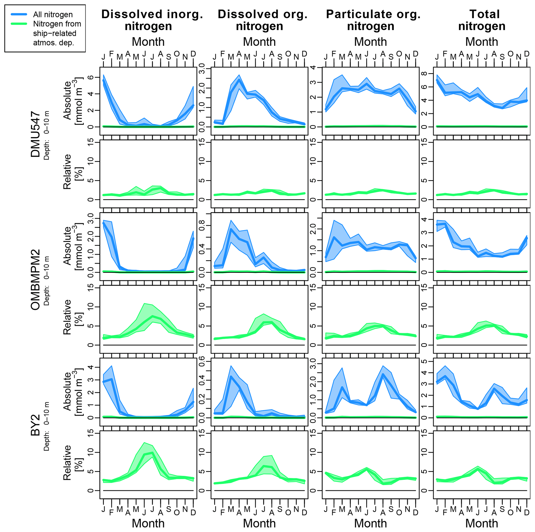
Figure 9Similar to Fig. 8 but showing monthly median and percentiles calculated from daily data at specific station locations (Fig. 8 shows monthly percentiles calculated from monthly mean data and shows the variability in space). The stations are the same as in the validation. A similar figure showing data at the other three stations is provided in the Supplement.
In the Belt Sea, the seasonal variability of the shipping contribution and its spatial variability are very low in all nitrogen fractions. The shipping contribution is between 1 % and 2 %. In the Öresund, it decreases from 1.5 % to 2 % in January to about 1 % in July and then increases again towards the end of the year. Finally, in the Arkona Basin, the shipping contribution increases from the beginning of the year until summer and then decreases. The values are in a range between 1 % and 4.5 %. However, there are some places in the Arkona Basin where the shipping contribution remains below 2 %.
Summarizing, the three considered basins represent three different regimes of shipping-related nitrogen deposition and of its contribution to the biogeochemical cycle. However, the relevance of shipping-related nitrogen differs spatially within each basin: the shipping contribution to the nitrogen fractions is much higher in the open ocean than along the coastline.
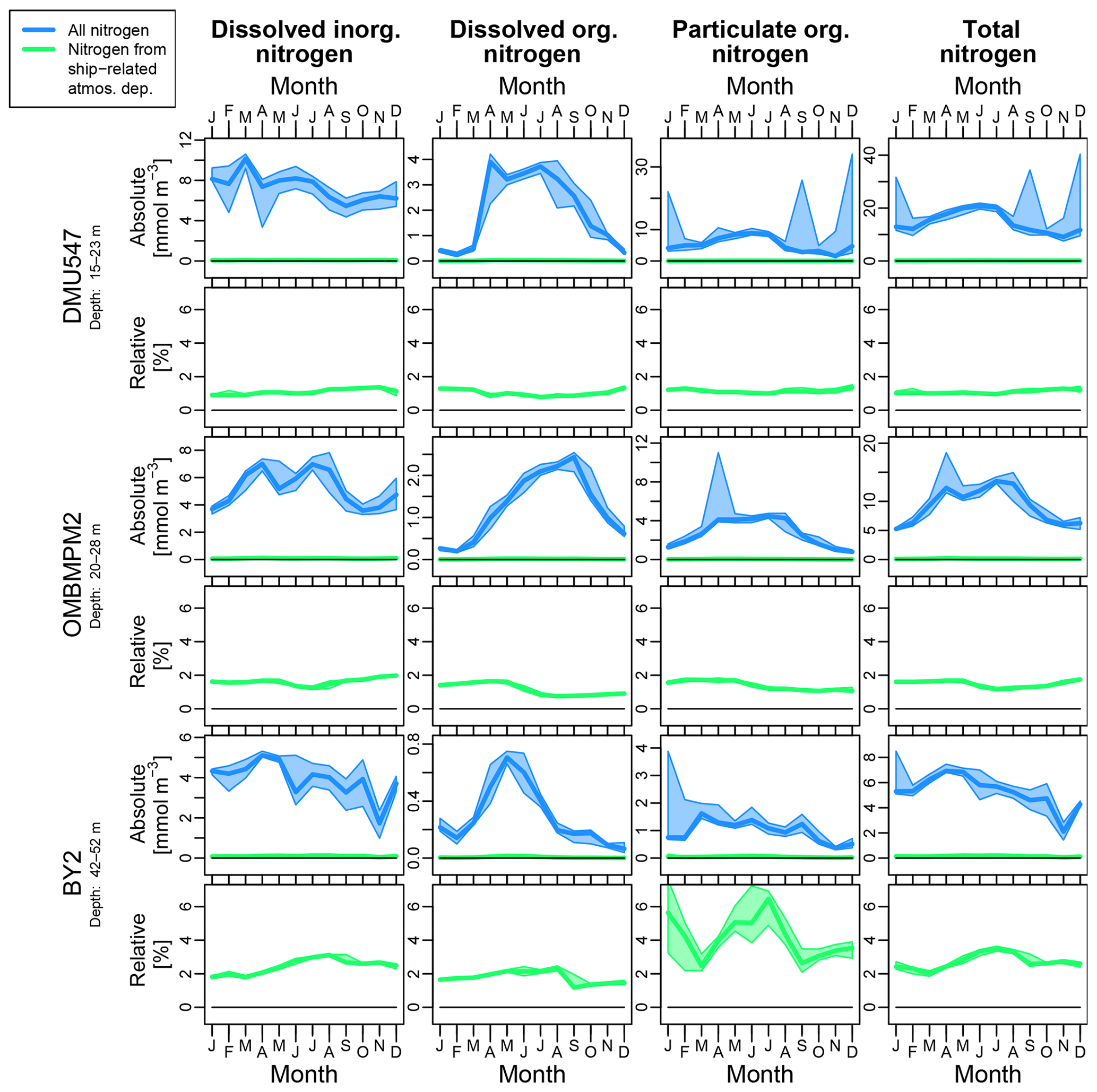
Figure 10Similar to Fig. 9 but for the bottom 8 to 10 m. The exact depth range is given on the left. A similar figure showing data at the other three stations is provided in the Supplement.
Figures 9 and 10 show the monthly median and percentiles calculated from daily mean values at the three stations (two of which are in the open ocean) in the surface and bottom layer, respectively. At the sea surface, the seasonal cycles of the DINall, DONall, and PONall concentrations are as expected. The time series of PONall and TNall concentrations shows two peaks: the first is the diatom bloom in spring and the second a cyanobacteria bloom in later summer. Cyanobacteria do not grow in the northern Belt Sea and Kattegat because the salinity is too high.
In the surface layer, the relative shipping contribution rises in all fractions and at all stations in spring, peaks in summer, and decreases again. At BY2, the PONship∕PONall ratio decreases after June and has a minimum in August, after which it increases again. The minimum is caused by the cyanobacteria bloom because the cyanobacteria fix non-tagged N2. The overall shipping contribution at DMU547 is similarly low as in the total basin. At OMBMPM2 and BY2, the TNship∕TNall ratio exceeds 5 %. At BY2, the DINship∕DINall ratio even exceeds 10 %. Thus, the shipping-related nitrogen contribution in summer is much higher at individual stations in the center of the basins than on basin average in the surface layer.
The shipping contribution to the nitrogen fractions is much lower in the bottom layer of the three stations. It remains below 2 % in all nitrogen fractions at DMU547 and OMBMPM2. At BY2, the contribution is higher than 2 % but still considerably lower than at the surface due to vertical stratification. The PONship∕PONall ratio peaks with ≈6 % at the bottom of BY2 in summer.
A vertically resolved meridional cross section through the Arkona Basin is evaluated in the next section (Sect. 3.4) in order to assess these differences between the surface and bottom layer concentrations at station BY2 in more detail.
3.4 Vertical distribution of shipping-related nitrogen in the Arkona Basin
In the previous sections, the spatial and temporal distribution of shipping-related nitrogen has been assessed. In this section, a cross section through the Arkona Basin is presented in order to evaluate the vertical distribution of shipping-related nitrogen.
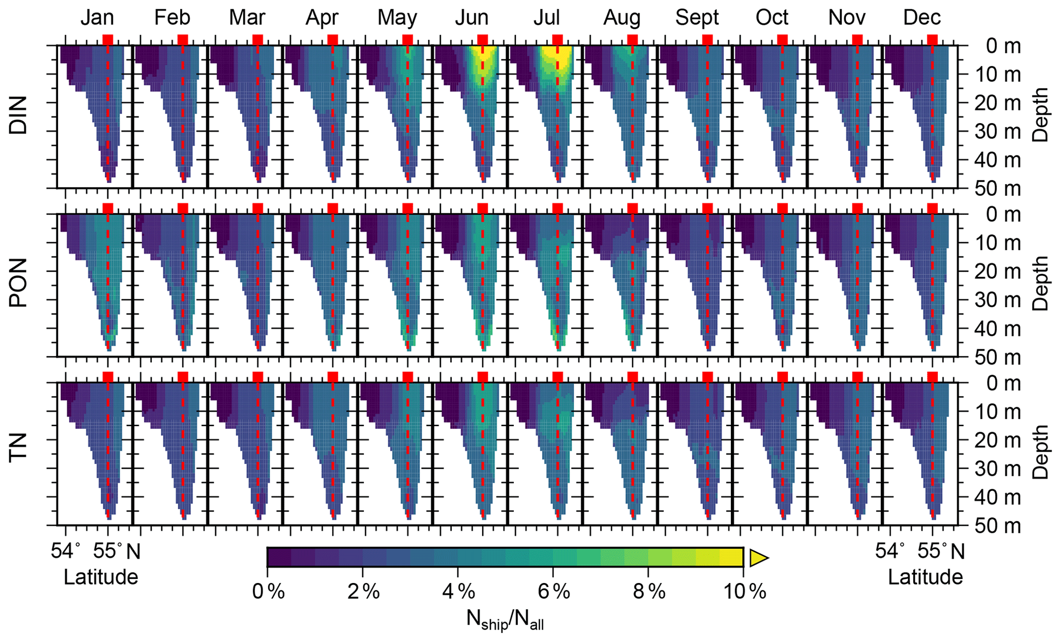
Figure 11Cross section at 14.08333∘ N through the Arkona Basin (red line in Fig. 3) showing the contribution of shipping nitrogen to all nitrogen in dissolved inorganic nitrogen (DIN, top) and total nitrogen (TN, bottom). Each column shows data for one month: January to December 2012 from left to right. The location of station BY2 is indicated by a red symbol at the sea surface. The vertical red dashed line represents the measurement profile taken at this station.
Figure 11 shows meridional cross sections of DIN, PON, and TN concentrations through the Arkona Basin along 14.0833∘ E.
In winter, the Arkona Basin is vertically well mixed. A horizontal gradient clearly exists, with low values in the south and high values in the north. In spring, the DINship∕DINall ratio increases in the central Arkona Basin at the sea surface and a vertical gradient develops; 1 to 2 months later, the TNship∕TNall ratio also develops a vertical gradient. This time lag is reasonable because a signal first appears in the DIN due to external DIN input and then spreads to PON and DON.
The surface layer DINship∕DINall ratio increases until July, exceeding 10 %, and then strongly decreases. The maximum of the TNship∕TNall is at the sea surface until June 2012 when it reaches 6 %. In the subsequent months, the maximum migrates downward and decreases. In July, the maximum is at ≈15 m of depth and amounts to ≈5.5 %. In August, it is at ≈20 m and amounts to ≈4.7 %. The downward migration is reasonable.
Detritus with a high shipping contribution sinks towards the seafloor as a result of the phytoplankton bloom in spring. In the open sea in early summer, the production of fresh PON decreases due to nutrient limitation. PON with a high content of non-shipping nitrogen is produced in coastal regions (nutrients supplied by rivers), is horizontally mixed from the coast towards the open sea, and sinks. As a result, the maximum of the PONship∕PONall ratio seems to be migrating downward (Fig. 11, top row). If the PON concentration is much higher than the DIN concentration, which is commonly the case in summer, the TNship∕TNall ratio will behave similarly to the PONship∕PONall ratio, as indicated by the bottom row of Fig. 11.
4.1 Discussion of the validation
The validation of simulation results showed a good agreement of physical and biogeochemical model data with in situ measurements (Fig. 5). The seasonal cycle was well reproduced. Modeled and concentrations deviated from measurements at the seafloor of station OMBMPM2 (Bay of Mecklenburg) in spring and autumn, respectively (Fig. 6).
Stations OMBMPN1 and OMBMPM (see the Supplement) show similar deviations in the nutrient concentrations at the seafloor as OMBMPM2. These stations are located northwestward and northeastward of OMBMPM2, respectively, close to the boundaries of the Bay of Mecklenburg. However, the deviations of modeled concentrations from measurements at these two stations are smaller than at OMBMPM2, indicating that mainly the Bay of Mecklenburg is affected.
MOM does not predict the vertical location of the halocline accurately in this region as we know from previous studies. This might affect the vertical transport – vertical mixing that is too weak– and lead to higher nutrient concentrations at the seafloor. Another reason might be that nutrients are released from the sediment into the water column in this region. The latter hypothesis cannot be tested because no sediment measurement data with high temporal resolution were available at this station.
The sea surface concentrations and their annual cycle seem to be well reproduced at all three stations – OMBMPM2, OMBMPN1, and OMBMPM. Hence, we assume that the observed deviations at the seafloor of the Bay of Mecklenburg do not negatively affect the general results of this study.
Very high PON and TN concentrations occurred at station DMU547 in September and December. These were caused by the resuspension of detritus through high current velocities at the seafloor (see plots in the Supplement for details).
4.2 Discussion of atmospheric nitrogen inputs
The wet deposition of oxidized and reduced nitrogen was systematically underestimated at Baltic Sea stations. The reported underestimation is consistent with the results of Vivanco et al. (2017). Nitrogen deposition in CMAQ simulations with very similar forcing data in the same region but in different years was evaluated. The reason for the underestimation could not be fully resolved in Karl et al. (2019a).
The deposition of untagged and shipping-related nitrogen was very high along the coastline. Particularly in bights and river estuaries, the nitrogen deposition was considerably high. This is partly of artificial origin and partly a result of specific atmospheric processes as we will describe below.
Atmospheric nitrogen deposition is higher above the land than above the ocean (Seinfeld and Pandis, 2016). Hence, there is a steep gradient in nitrogen deposition away from the coastline. The coarser horizontal grid resolution of the CMAQ setup compared to the MOM–ERGOM setup and subsequent interpolation of nitrogen deposition data over the land–sea interface cause a smoothing of nitrogen deposition in this region, leading to artificially enhanced deposition into the coastal waters.
The second reason, which is non-artificial, is probably the interaction in the atmosphere between nitrogen oxides (NOX) from shipping, ammonia (NH3) from agricultural activities and animal livestock, and sea salt particles emitted from the sea surface. Although this topic is not in the focus of this study, we describe some details in the subsequent paragraphs.
NOX reacts to HNO3. HNO3 condenses on wet particles and reduces the pH of the particle water (Reaction R1). NH3 condenses on wet particles and increases the pH of the particle water (Reaction R2). Both processes are equilibrium processes. When both processes take place at the same time, the pH is kept on a roughly constant level, shifting the equilibrium towards the right side of Reaction (R3).
Additionally, sodium chloride (NaCl; ) favors the condensation and deprotonation of atmospheric acids, such as HNO3 (Reaction R4). The condensation of HNO3 reduces the pH of the particle water. Hydrochloric acid (HCl) is a weaker acid than HNO3. Hence, Cl− has a higher probability to accept a proton (and to evaporate subsequently) than .
Sea salt emissions considerably contribute to the atmospheric particle load in the vicinity of the shoreline and favor the formation of particulate nitrogen compounds. Sea salt particles are relatively large and hence have a short atmospheric residence time, meaning they are quickly deposited. Therefore, shipping-related nitrogen deposition is expected to be enhanced in some coastal regions through the interaction of shipping-related NOX and sea salt particles.
4.3 Discussion of the shipping contribution
The concentration of shipping-related total nitrogen (TNship) was relatively homogeneously distributed horizontally (Fig. 7). A few coastal regions showed increased TNship concentrations. Relatively, the contribution of shipping-related nitrogen to TN (TNship∕TNall) was highest distant from the coast. The pattern agrees with regions of high shipping activity. This is a coincidence with no interdependence. This agreement results not from shipping activity but rather from the lack of riverine nitrogen sources in offshore regions.
In the surface waters of the Arkona Basin and the Bay of Mecklenburg, the shipping contribution to all nitrogen fractions was highest in summer and lowest in winter (Fig. 8). The contribution of shipping-related nitrogen to particulate organic nitrogen (PONship∕PONall) strongly decreased in the Arkona Basin in August, caused by a cyanobacteria bloom. In the bottom water, the shipping contribution was quite constant over the entire year due to stable vertical stratification during the bloom period. An exception was PONship∕PONall in summer in the bottom water of station BY2, which is located in the center of the Arkona Basin (Fig. 10). This is discussed further below.
In the Öresund, the annual cycle of the shipping contribution to all nitrogen fractions was inverted to the cycle in the Arkona Basin (Fig. 8). In the summer, the cycle shows a minimum in the Öresund and a maximum in the Arkona Basin. Particularly in summer, atmospheric deposition is an important nutrient source for large basins such as the Arkona Basin. The fraction between sea surface area and coastline length is lower in the Öresund than in the Arkona Basin. Moreover, the Öresund is considerably impacted by nutrient loads from the Swedish mainland and from Zealand (Mølleåen River). This leads to a lower relevance of atmospheric nitrogen deposition compared to riverine nutrient loads, causing the inverted annual cycle.
No clear annual cycle was recognizable in the Belt Sea. The Belt Sea is a quite diverse and complex region. Hence, one can expect that the shipping-contribution is not uniform over the whole water body of the Belt Sea. Thus, one might split the Belt Sea into several regions in future studies.
A vertically resolved meridional cross section through the Arkona Basin was analyzed. During the algal bloom period, the contribution of shipping-related N to DIN (DINship∕DINall) was highest at the sea surface in the center of the Arkona Basin and decreased vertically downward (Fig. 11). During other times of the year, it showed a weak vertical gradient. The DINship∕DINall ratio decreased from the center of the Arkona towards the coast, particularly towards the south. The Oder River is located in the south, contributing large amounts of riverine DIN and hence causing the low DINship∕DINall values.
The maximum of TNship∕TNall and PONship∕PONall was at the sea surface until June and afterwards moved downwards due to large amounts of sinking detritus with shipping-related nitrogen. This caused the high PONship∕PONall ratio at the seafloor at station BY2 (Fig. 10).
4.4 Comparison to other studies
Raudsepp et al. (2013) and Raudsepp et al. (2019) performed similar studies. Raudsepp et al. (2013) focused on the impact of shipping-related nitrogen deposition on nitrogen fixation by cyanobacteria in the Gulf of Finland. Raudsepp et al. (2019) assessed the impact of shipping-related nutrient inputs (direct discharge and deposition of atmospheric emissions; nitrogen and phosphorus) on the biogeochemical system in the whole Baltic Sea with a focus on HELCOM station BY15 in the eastern Gotland Basin. The authors did not tag shipping-related nitrogen but performed two simulations, one with and another one without the shipping nitrogen contribution, and calculated the difference. Raudsepp et al. (2019) used the same atmospheric deposition dataset, which was a comparable ERGOM version but another ocean circulation model. Hence, the year 2012 was also assessed.
Raudsepp et al. (2019) found an increase in shipping-related nitrogen in , diatoms, and flagellates in early summer followed by a steep decline in late summer, which is caused by a cyanobacteria bloom. This result is comparable to this study's result at BY2 where the cyanobacteria bloom had a similar effect. At the other two stations in this study the physical conditions do not allow for cyanobacteria blooms and hence do not show this result. The spatial pattern of the contribution of shipping nitrogen to and DIN in Raudsepp et al. (2019) and in this study, respectively, is very similar with respect to increased shipping nitrogen in some coastal regions. This can be expected due to similar nitrogen deposition datasets.
In this study, shipping-related nitrogen was tagged in one simulation. The biogeochemical system behaved in the same way as when shipping-related nitrogen had not been tagged. In contrast, two simulations with and without shipping-related nitrogen inputs were performed in Raudsepp et al. (2019). The results were subtracted from each other in a second step and the difference was evaluated (the “difference approach”). The two simulations might reveal different system dynamics because the biogeochemical system is a complex nonlinear system. Hence, the results of this study are not one-to-one comparable to those of Raudsepp et al. (2019).
Both approaches to assess the contribution of shipping activities to the nitrogen cycle are valid but should be used for different research questions. The difference approach by Raudsepp et al. (2019) is very useful when we want to assess what would happen if shipping emissions are reduced or totally avoided. The system behavior might change in this situation, and hence two distinct simulations should be performed. The tagging approach would not capture the nonlinear changes in the system behavior. In contrast, the tagging approach is reasonable when we want to assess the contribution of one or more nutrient sources to state variables in the current situation. We are mainly interested in the latter aspect and have hence chosen the tagging approach in this study.
Following Raudsepp et al. (2013), Neumann et al. (2018), and Raudsepp et al. (2019) this is the fourth study dealing with tracing shipping-related nitrogen inputs in the Baltic Sea biogeochemical system. This study focused on the western Baltic Sea using a state-of-the-art biogeochemical model.
The absolute contribution of the shipping sector to TN was highest along the shoreline, which was caused by the interaction of shipping-related NOX with sea salt particles and ammonia in the atmosphere and subsequent dry deposition. However, the relative contribution of the shipping sector to TN showed an inverted pattern: the lowest contribution along the shoreline and increasing towards the open sea. Riverine nutrient inputs led to a relatively low relevance of atmospheric shipping-related inputs along the shoreline . Hence, offshore regions rather than coastal regions might benefit from reduced inputs of shipping-related nitrogen.
The contribution of shipping-related nitrogen to TN was below 5 % on a large scale on annual average. Hence, measures like nitrogen emission control areas, which limit the NOX emissions of ships, are expected to have a low impact on eutrophication on a large scale. However, the shipping contribution to TN exceeded 5 % in the centers of the basins in summer. The shipping-related DIN was even in a range between 10 % and 15 % in the center of the Arkona Basin. Hence, the shipping sector – and atmospheric deposition in general – is an important nutrient source in offshore regions in summer.
The vertical distribution of nitrogen indicated that the sinking of detritus leads to the transport of shipping-related nitrogen into sediment. An assessment of the sedimentary nitrogen composition is not reasonable in this study due to the simple sediment parameterization used. Hence, it is not clear what part of shipping-related nitrogen is buried in the sediment and what part is released back into the water column, either as bioavailable nitrogen or as N2. Future studies should focus on the sediment, i.e., with a more sophisticated sediment model.
The contribution of shipping-related nitrogen to TN seems to be low, taking values below 5 % on average. However, we do not have comparable numbers of the contribution of other atmospheric nitrogen emission source sectors, i.e., road traffic (NOX), power production (NOX), and livestock farming (ammonia ∕ ammonium, ). In this context, this study is rather one case study. Future studies should target several source sectors in order to put the relative contributions of individual source sectors into context.
Code. The original MOM code is accessible via the MOM GitHub repository (https://mom-ocean.github.io/, last access: 10 January 2020). The ERGOM code and a description of the model processes and constants are attached in the Supplement. The latest ERGOM version, which might differ from the version used in this study, is available via the ERGOM home page (https://ergom.net, last access: 10 January 2020). Information on the technical aspects of coupling ERGOM to MOM is provided on request.
Model output data. The model output data are published at the World Data Center for Climate Data (WDCC) of the German Climate Computing Center (DKRZ, Deutsches Klimarechenzentrum; https://doi.org/10.26050/WDCC/MOMERGOMBSCMAQ) (Neumann et al., 2019).
Model input data.
-
The meteorological input data for MOM–ERGOM were taken from the coastDat2 database of the Helmholtz-Zentrum Geesthacht (https://www.coastdat.de/; Geyer and Rockel, 2013). The data are available at the WDCC of the DKRZ (https://doi.org/10.1594/WDCC/coastDat-2_COSMO-CLM; Geyer and Rockel, 2013).
-
The CMAQ nitrogen deposition data are available upon request from the coauthors of the HZG. Some results of the CMAQ simulations are available via the SHEBA THREDDS server at http://sheba.hzg.de/thredds/catalog/publicAll/WP2-Air/catalog.html (last access: 10 January 2020).
Measurement data.
-
HELCOM data are available via the ICES home page: http://ocean.ices.dk/helcom/Helcom.aspx (HELCOM, 2019).
-
IOWDB data are available on request (https://www.io-warnemuende.de/iowdb.html, HZG, 2019). Please contact the authors for access to the database.
The supplement related to this article is available online at: https://doi.org/10.5194/os-16-115-2020-supplement.
DN was responsible for the overall structure and for writing the paper. He performed the MOM–ERGOM model simulations and did major programming and plotting tasks. HR implemented the tagging method and a tool for model validation. He contributed to the “Materials and methods” and Discussion sections. MK performed CMAQ air quality model simulations and evaluated meteorological forcing data and nitrogen deposition data. He contributed to the “Materials and methods” and Discussion sections. He further helped develop the research questions. VM contributed to the state of knowledge, to the Introduction section, and to the development of the research questions. He further provided input data for the CMAQ model simulations. RF provided measurement data, participated in the evaluation of the model data, and contributed to the Results and Discussion sections. TN supported the development of the research questions, contributed to the Introduction, “Materials and methods”, and Conclusions sections, and is the lead developer of ERGOM.
The authors declare that they have no conflict of interest.
This article is part of the special issue “Shipping and the Environment – From Regional to Global Perspectives (ACP/OS inter-journal SI)”. It is a result of the Shipping and the Environment – From Regional to Global Perspectives, Gothenburg, Sweden, 23–24 October 2017.
The MOM–ERGOM model simulations were performed at the cluster Konrad of the North-German Supercomputing Alliance (HLRN, project ID mvk00054) within MeRamo. The meteorological and atmospheric chemistry transport model (CTM) simulations were performed for SHEBA at the German Climate Computing Center (DKRZ) within the Project “Regionale Atmosphärenmodellierung” (project ID 302), which is funded by the Helmholtz Association. The emissions for the CTM simulations were kindly provided by Johannes Bieser, Armin Aulinger, and Jukka-Pekka Jalkanen. The meteorological input data for the MOM–ERGOM simulations were taken from the CCLM coastDat2 dataset by Beate Geyer. MOM has been developed and is maintained by the Geophysical Fluid Dynamics Laboratory (GFDL), which is part of the U.S. National Oceanographic and Atmospheric Agency (NOAA). The air quality model is developed and maintained by the U.S. Environmental Protection Agency (US EPA). We thank our colleagues conducting IOW's Baltic monitoring and long-term data program, whose intensively quality-checked measurements we used for the model validation. Additional measurement data were kindly provided by the HELCOM oceanographic measurements database hosted by ICES. We thank Uwe Schulzweida, Charlie Zender, Paul Wessel, the R Core Team, and the Unidata development team (and all involved developers and contributors) for maintaining the open-source software packages Climate Data Operators (CDO), the NetCDF Operators (NCO), Generic Mapping Tools (GMT), the statistical computing language R, and NetCDF, respectively.
This research has been supported by the European Commission (BONUS SHEBA project), the German Federal Ministry for Transport and Digital Infrastructure (BMVI; MeRamo Project, FKZ 50EW1601), and the German Federal Ministry of Education and Research (BMBF; PROSO Project, FKZ 03F0779A). The publication of this article will also be funded by the SHEBA project. If the entire publication cost is not covered by SHEBA, the remaining costs will be paid by the Leibniz Publication Fund.
The publication of this article was funded by the
Open Access Fund of the Leibniz Association.
This paper was edited by David Turner and reviewed by Fabian Große and one anonymous referee.
Aksoyoglu, S., Baltensperger, U., and Prévôt, A. S. H.: Contribution of ship emissions to the concentration and deposition of air pollutants in Europe, Atmos. Chem. Phys., 16, 1895–1906, https://doi.org/10.5194/acp-16-1895-2016, 2016. a
Andersen, J. H., Halpern, B. S., Korpinen, S., Murray, C., and Reker, J.: Baltic Sea biodiversity status vs. cumulative human pressures, Estuar. Coast. Shelf Sci., 161, 88–92, https://doi.org/10.1016/j.ecss.2015.05.002, 2015. a
Andersen, J. H., Carstensen, J., Conley, D. J., Dromph, K., Fleming-Lehtinen, V., Gustafsson, B. G., Josefson, A. B., Norkko, A., Villnäs, A., and Murray, C.: Long-term temporal and spatial trends in eutrophication status of the Baltic Sea, Biol. Rev., 92, 135–149, https://doi.org/10.1111/brv.12221, 2017. a
Appel, K. W., Napelenok, S. L., Foley, K. M., Pye, H. O. T., Hogrefe, C., Luecken, D. J., Bash, J. O., Roselle, S. J., Pleim, J. E., Foroutan, H., Hutzell, W. T., Pouliot, G. A., Sarwar, G., Fahey, K. M., Gantt, B., Gilliam, R. C., Heath, N. K., Kang, D., Mathur, R., Schwede, D. B., Spero, T. L., Wong, D. C., and Young, J. O.: Description and evaluation of the Community Multiscale Air Quality (CMAQ) modeling system version 5.1, Geosci. Model Dev., 10, 1703–1732, https://doi.org/10.5194/gmd-10-1703-2017, 2017. a
Bartnicki, J. and Fagerli, H.: Airborne load of nitrogen to European seas, Ecol. Chem. Eng. S., 15, 297–313, 2008. a, b
Bartnicki, J., Semeena, V. S., and Fagerli, H.: Atmospheric deposition of nitrogen to the Baltic Sea in the period 1995–2006, Atmos. Chem. Phys., 11, 10057–10069, https://doi.org/10.5194/acp-11-10057-2011, 2011. a
Bieser, J., Aulinger, A., Matthias, V., Quante, M., and Builtjes, P.: SMOKE for Europe – adaptation, modification and evaluation of a comprehensive emission model for Europe, Geosci. Model Dev., 4, 47–68, https://doi.org/10.5194/gmd-4-47-2011, 2011. a
Binkowski, F. S. and Roselle, S. J.: Models-3 Community Multiscale Air Quality (CMAQ) model aerosol component 1. Model description, J. Geophys. Res.-Atmos., 108, 4183, https://doi.org/10.1029/2001JD001409, 2003. a
Binkowski, F. S. and Shankar, U.: The Regional Particulate Matter Model: 1. Model description and preliminary results, J. Geophys. Res.-Atmos., 100, 26191–26209, https://doi.org/10.1029/95JD02093, 1995. a
Brandt, J., Silver, J. D., Christensen, J. H., Andersen, M. S., Bønløkke, J. H., Sigsgaard, T., Geels, C., Gross, A., Hansen, A. B., Hansen, K. M., Hedegaard, G. B., Kaas, E., and Frohn, L. M.: Assessment of Health-Cost Externalities of Air Pollution at the National Level using the EVA Model System, CEEH Scientific Report No 3, Tech. rep., Centre for Energy, Environment and Health, 2011. a
Buhaug, O., Corbett, J. J., Endresen, O., Eyring, V., Faber, J., Hanayama, S., Lee, D., Lee, D., Lindstad, H., Markowaka, A., Mjelde, A., Nelissen, D., Nilsen, J., Palsson, C., Winebrake, J., Wu, W., and Yoshida, K.: Second IMO GHG study, Tech. rep., IMO, available at: http://www.imo.org/en/OurWork/Environment/PollutionPrevention/AirPollution/Documents/SecondIMOGHGStudy2009.pdf (last access: 13 January 2020), 2009. a
CEIP: WebDab Emission Export of the EU-28 countries divided into SNAP sectors, available at: https://www.ceip.at/webdab-emission-database (last access: 13 January 2020), 2018. a
Danish EPA: Economic Impact Assessment of a NOx Emission Control Area in the North Sea, Tech. rep., Danish EPA, available at: https://www2.mst.dk/Udgiv/publications/2012/06/978-87-92903-20-4.pdf (last access: 13 January 2020), 2012. a
Dulière, V., Gypens, N., Lancelot, C., Luyten, P., and Lacroix, G.: Origin of nitrogen in the English Channel and Southern Bight of the North Sea ecosystems, Hydrobiologia, 845, 13–33, https://doi.org/10.1007/s10750-017-3419-5, 2017. a
EMEP: EMEP Status Report 1/2014 “Transboundary particulate matter, photo-oxidants, acidifying and eutrophying components”, Joint msc-w & ccc & ceip report, MSC-W & CCC & CEIP, available at: http://emep.int/publ/reports/2014/EMEP_Status_Report_1_2014.pdf (last access: 13 January 2020), 2014. a, b, c
EMEP: EMEP Status Report 1/2017 “Transboundary particulate matter, photo-oxidants, acidifying and eutrophying components”, Joint msc-w & ccc & ceip report, MSC-W & CCC & CEIP, available at: http://emep.int/publ/reports/2017/EMEP_Status_Report_1_2017.pdf (last access: 13 January 2020), 2017. a
EU-2008/56/EC: Directive 2008/56/EC of the European Parliament and of the Council on establishing a framework for community action in the field of marine environmental policy (Marine Strategy Framework Directive), Official Journal of the European Union, available at: http://eur-lex.europa.eu/legal-content/EN/TXT/?uri=CELEX:32008L0056 (last access: 13 January 2020), 2008. a
Feistel, R., Nausch, G., and Wasmund, N. (Eds.): State and Evolution of the Baltic Sea, 1952–2005, Wiley-Interscience, Hoboken, New Jersey, 1st edn., https://doi.org/10.1002/9780470283134, 2008. a, b
Foley, K. M., Roselle, S. J., Appel, K. W., Bhave, P. V., Pleim, J. E., Otte, T. L., Mathur, R., Sarwar, G., Young, J. O., Gilliam, R. C., Nolte, C. G., Kelly, J. T., Gilliland, A. B., and Bash, J. O.: Incremental testing of the Community Multiscale Air Quality (CMAQ) modeling system version 4.7, Geosci. Model Dev., 3, 205–226, https://doi.org/10.5194/gmd-3-205-2010, 2010. a
Fountoukis, C. and Nenes, A.: ISORROPIA II: a computationally efficient thermodynamic equilibrium model for K+–Ca2+–Mg2+––Na+–––Cl−–H2O aerosols, Atmos. Chem. Phys., 7, 4639–4659, https://doi.org/10.5194/acp-7-4639-2007, 2007. a
Geels, C., Hansen, K. M., Christensen, J. H., Ambelas Skjøth, C., Ellermann, T., Hedegaard, G. B., Hertel, O., Frohn, L. M., Gross, A., and Brandt, J.: Projected change in atmospheric nitrogen deposition to the Baltic Sea towards 2020, Atmos. Chem. Phys., 12, 2615–2629, https://doi.org/10.5194/acp-12-2615-2012, 2012. a, b
Geyer, B.: High-resolution atmospheric reconstruction for Europe 1948–2012: coastDat2, Earth Syst. Sci. Data, 6, 147–164, https://doi.org/10.5194/essd-6-147-2014, 2014. a
Geyer, B. and Rockel, B.: coastDat-2 COSMO-CLM Atmospheric Reconstruction, World Data Center for Climate (WDCC), Hamburg, Germany, https://doi.org/10.1594/WDCC/coastDat-2_COSMO-CLM, 2013. a, b, c
Geyer, B., Weisse, R., Bisling, P., and Winterfeldt, J.: Climatology of North Sea wind energy derived from a model hindcast for 1958-2012, J. Wind Eng. Ind. Aerod., 147, 18–29, https://doi.org/10.1016/j.jweia.2015.09.005, 2015. a
Gong, S. L.: A parameterization of sea-salt aerosol source function for sub- and super-micron particles, Global Biogeochem. Cy., 17, 1097, https://doi.org/10.1029/2003GB002079, 2003. a
Griffies, S. M.: Fundamentals of Ocean Climate Models, Princeton University Press, Princeton, New Jersey, available at: https://press.princeton.edu/titles/7797.html (last access: 13 January 2020), 2004. a
Große, F., Kreus, M., Lenhart, H.-J., Pätsch, J., and Pohlmann, T.: A Novel Modeling Approach to Quantify the Influence of Nitrogen Inputs on the Oxygen Dynamics of the North Sea, Front. Mar. Sci., 4, 383, https://doi.org/10.3389/fmars.2017.00383, 2017. a
Gustafsson, B. G., Schenk, F., Blenckner, T., Eilola, K., Meier, H. E. M., Müller-Karulis, B., Neumann, T., Ruoho-Airola, T., Savchuk, O. P., and Zorita, E.: Reconstructing the Development of Baltic Sea Eutrophication 1850–2006, AMBIO, 41, 534–548, https://doi.org/10.1007/s13280-012-0318-x, 2012. a
Hammingh, P., Holland, M., Geilenkirchen, G., Jonson, J., and Maas, R.: Assessment of the environmental impacts and health benefits of a nitrogen emission control area in the North Sea, Tech. Rep. 500249001, PBL Netherlands Environmental Assessment Agency, 2012. a
HELCOM: Airborne nitrogen loads to the Baltic Sea, Tech. rep., Helsinki Commission, Baltic Marine Environment Protection Commission, available at: https://www.helcom.fi/wp-content/uploads/2019/08/Airborne-nitrogen-loads-to-the-Baltic-Sea.pdf (last access: 13 January 2020), 2005. a, b, c
HELCOM: Baltic Sea Action Plan (BSAP), Tech. rep., HELCOM, available at: http://www.helcom.fi/baltic-sea-action-plan (last access: 13 January 2020), 2007. a
HELCOM: Eutrophication in the Baltic Sea – An integrated thematic assessment of the effects of nutrient enrichment and eutrophication in the Baltic Sea region, Balt. sea environ. proc. no. 115b, HELCOM, available at: http://www.helcom.fi/Lists/Publications/BSEP115B.pdf (last access: 13 January 2020), 2009. a
HELCOM (Ed.): Approaches and methods for eutrophication target setting in the Baltic Sea region, no. 133 in Balt, Sea Environ. Proc. No., available at: http://www.helcom.fi/Lists/Publications/BSEP133.pdf (last access: 13 January 2020), 2013a. a, b
HELCOM (Ed.): Review of the Fifth Baltic Sea Pollution Load Compilation for the 2013 HELCOM Ministerial Meeting, no. 141 in Balt. Sea Environ. Proc. No., available at: http://www.helcom.fi/Lists/Publications/BSEP141.pdf (last access: 13 January 2020), 2013b. a, b, c
HELCOM: Summary report on the development of revised maximum allowable inputs (mai) and updated country allocated reduction targets (cart) of the baltic sea action plan., Tech. rep., Helcom, available at: https://helcom.fi/media/documents/Summary-report-on-MAI-CART-1.pdf (last access: 13 January 2020), 2013c. a
HELCOM: Updated Fifth Baltic Sea Pollution Load Compilation (PLC-5.5), Baltic Sea Environment Proceedings 145, HELCOM, available at: http://www.helcom.fi/Lists/Publications/BSEP145_Lowres.pdf (last access: 13 January 2020), 2015. a
HELCOM: HELCOM oceanographic data – Baltic Sea Monitoring data, ICES, Copenhagen, available at: https://ocean.ices.dk/helcom/Helcom.aspx (last access: 10 January 2020), 2019. a
Hongisto, M.: Impact of the emissions of international sea traffic on airborne deposition to the Baltic Sea and concentrations at the coastline, Oceanologia, 56, 349–372, https://doi.org/10.5697/oc.56-2.349, 2014. a
HZG: coastDat-3 COSMO-CLM Atmospheric Reconstruction, World Data Center for Climate (WDCC), Hamburg, Germany, available at: http://cera-www.dkrz.de/WDCC/ui/Compact.jsp?acronym=coastDat-3_COSMO-CLM_ERAi (last access: 13 January 2020), 2017. a, b
IOWDB: The oceanographic database of the IOW, Leibniz Institute for Baltic Sea Research, Rostock, Warnemünde, https://www.io-warnemuende.de/iowdb.html (last access: 2020-01-10), 2019. a
Jalkanen, J.-P., Johansson, L., Kukkonen, J., Brink, A., Kalli, J., and Stipa, T.: Extension of an assessment model of ship traffic exhaust emissions for particulate matter and carbon monoxide, Atmos. Chem. Phys., 12, 2641–2659, https://doi.org/10.5194/acp-12-2641-2012, 2012. a
Jonson, J. E., Jalkanen, J. P., Johansson, L., Gauss, M., and Denier van der Gon, H. A. C.: Model calculations of the effects of present and future emissions of air pollutants from shipping in the Baltic Sea and the North Sea, Atmos. Chem. Phys., 15, 783–798, https://doi.org/10.5194/acp-15-783-2015, 2015. a, b
Karl, M., Bieser, J., Geyer, B., Matthias, V., Jalkanen, J.-P., Johansson, L., and Fridell, E.: Impact of a nitrogen emission control area (NECA) on the future air quality and nitrogen deposition to seawater in the Baltic Sea region, Atmos. Chem. Phys., 19, 1721–1752, https://doi.org/10.5194/acp-19-1721-2019, 2019a. a, b, c, d
Karl, M., Jonson, J. E., Uppstu, A., Aulinger, A., Prank, M., Sofiev, M., Jalkanen, J.-P., Johansson, L., Quante, M., and Matthias, V.: Effects of ship emissions on air quality in the Baltic Sea region simulated with three different chemistry transport models, Atmos. Chem. Phys., 19, 7019–7053, https://doi.org/10.5194/acp-19-7019-2019, 2019b. a
Kelly, J. T., Bhave, P. V., Nolte, C. G., Shankar, U., and Foley, K. M.: Simulating emission and chemical evolution of coarse sea-salt particles in the Community Multiscale Air Quality (CMAQ) model, Geosci. Model Dev., 3, 257–273, https://doi.org/10.5194/gmd-3-257-2010, 2010. a
Korpinen, S., Meski, L., Andersen, J. H., and Laamanen, M.: Human pressures and their potential impact on the Baltic Sea ecosystem, Ecol. Indic., 15, 105–114, https://doi.org/10.1016/j.ecolind.2011.09.023, 2012. a
Kuznetsov, I. and Neumann, T.: Simulation of carbon dynamics in the Baltic Sea with a 3D model, J. Mar. Syst., 111–112, 167–174, https://doi.org/10.1016/j.jmarsys.2012.10.011, 2013. a
Los, F., Troost, T., and Beek, J. V.: Finding the optimal reduction to meet all targets – Applying Linear Programming with a nutrient tracer model of the North Sea, J. Mar. Syst., 131, 91–101, https://doi.org/10.1016/j.jmarsys.2013.12.001, 2014. a
Matthias, V., Aulinger, A., Backes, A., Bieser, J., Geyer, B., Quante, M., and Zeretzke, M.: The impact of shipping emissions on air pollution in the greater North Sea region – Part 2: Scenarios for 2030, Atmos. Chem. Phys., 16, 759–776, https://doi.org/10.5194/acp-16-759-2016, 2016. a
Ménesguen, A., Cugier, P., and Leblond, I.: A new numerical technique for tracking chemical species in a multi-source, coastal ecosystem, applied to nitrogen causing Ulva blooms in the Bay of Brest (France), Limnol. Oceanogr., 51, 591–601, https://doi.org/10.4319/lo.2006.51.1_part_2.0591, 2006. a
Ménesguen, A., Desmit, X., Dulière, V., Lacroix, G., Thouvenin, B., Thieu, V., and Dussauze, M.: How to avoid eutrophication in coastal seas? A new approach to derive river-specific combined nitrate and phosphate maximum concentrations, Sci. Total Environ., 628–629, 400–414, https://doi.org/10.1016/j.scitotenv.2018.02.025, 2018. a
Nausch, M., Woelk, J., Kahle, P., Nausch, G., Leipe, T., and Lennartz, B.: Phosphorus fractions in discharges from artificially drained lowland catchments (Warnow River, Baltic Sea), Agric. Water Manage., 187, 77–87, https://doi.org/10.1016/j.agwat.2017.03.006, 2017. a
Neumann, D., Matthias, V., Bieser, J., Aulinger, A., and Quante, M.: Sensitivity of modeled atmospheric nitrogen species and nitrogen deposition to variations in sea salt emissions in the North Sea and Baltic Sea regions, Atmos. Chem. Phys., 16, 2921–2942, https://doi.org/10.5194/acp-16-2921-2016, 2016. a, b
Neumann, D., Matthias, V., Bieser, J., Aulinger, A., and Quante, M.: Sensitivity of modeled atmospheric nitrogen species and nitrogen deposition to variations in sea salt emissions in the North Sea and Baltic Sea regions, Atmos. Chem. Phys., 16, 2921–2942, https://doi.org/10.5194/acp-16-2921-2016, 2016. a
Neumann, D., Karl, M., Radtke, H., and Neumann, T.: MOM-ERGOM western Baltic Sea simulations with tagging of atmospheric nitrogen deposition by CMAQ, World Data Center for Climate (WDCC) at DKRZ, https://doi.org/10.26050/WDCC/MOMERGOMBSCMAQ, 2019. a
Neumann, T.: Towards a 3D-ecosystem model of the Baltic Sea, J. Mar. Syst., 25, 405–419, https://doi.org/10.1016/S0924-7963(00)00030-0, 2000. a
Neumann, T.: The fate of river-borne nitrogen in the Baltic Sea – An example for the River Oder, Estuar. Coast. Shelf Sci., 73, 1–7, https://doi.org/10.1016/j.ecss.2006.12.005, 2007. a
Neumann, T. and Schernewski, G.: Eutrophication in the Baltic Sea and shifts in nitrogen fixation analyzed with a 3D ecosystem model, J. Mar. Syst., 74, 592–602, https://doi.org/10.1016/j.jmarsys.2008.05.003, 2008. a
Neumann, T., Fennel, W., and Kremp, C.: Experimental simulations with an ecosystem model of the Baltic Sea: A nutrient load reduction experiment, Global Biogeochem. Cy., 16, 1–19, https://doi.org/10.1029/2001GB001450, 2002. a, b
Neumann, T., Siegel, H., and Gerth, M.: A new radiation model for Baltic Sea ecosystem modelling, J. Mar. Syst., 152, 83–91, https://doi.org/10.1016/j.jmarsys.2015.08.001, 2015. a, b
Neumann, T., Radtke, H., and Seifert, T.: On the importance of Major Baltic Inflows for oxygenation of the central Baltic Sea, J. Geophys. Res.-Oceans, 122 1090–1101, https://doi.org/10.1002/2016JC012525, 2017. a
Nolte, C. G., Appel, K. W., Kelly, J. T., Bhave, P. V., Fahey, K. M., Collett Jr., J. L., Zhang, L., and Young, J. O.: Evaluation of the Community Multiscale Air Quality (CMAQ) model v5.0 against size-resolved measurements of inorganic particle composition across sites in North America, Geosci. Model Dev., 8, 2877–2892, https://doi.org/10.5194/gmd-8-2877-2015, 2015. a
Omstedt, A., Gustafsson, B., Rodhe, J., and Walin, G.: Use of Baltic Sea modelling to investigate the water cycle and the heat balance in GCM and regional climate models, Climate Res., 15, 95–108, 2000. a, b
Paerl, H. W., Dennis, R. L., and Whitall, D. R.: Atmospheric deposition of nitrogen: Implications for nutrient over-enrichment of coastal waters, Estuaries, 25, 677–693, https://doi.org/10.1007/BF02804899, 2002. a
Pleim, J., Venkatram, A., and Yamartino, R.: ADOM/TADAP model development program 4: The dry deposition module, Tech. rep., Ontario Ministry of the Environment Toronto, Canada, 1984. a
Radtke, H., Neumann, T., Voss, M., and Fennel, W.: Modeling pathways of riverine nitrogen and phosphorus in the Baltic Sea, J. Geophys. Res.-Oceans, 117, c09024, https://doi.org/10.1029/2012JC008119, 2012. a, b, c
Radtke, H., Neumann, T., and Fennel, W.: A Eulerian nutrient to fish model of the Baltic Sea – A feasibility-study, J. Mar. Syst., 125, 61–76, https://doi.org/10.1016/j.jmarsys.2012.07.010, 2013. a
Raudsepp, U., Laanemets, J., Maljutenko, I., Hongisto, M., and Jalkanen, J.-P.: Impact of ship-borne nitrogen deposition on the Gulf of Finland ecosystem: an evaluation, Oceanologia, 55, 837–857, https://doi.org/10.5697/oc.55-4.837, 2013. a, b, c, d
Raudsepp, U., Maljutenko, I., outs, M. K., Granhag, L., Wilewska-Bien, M., Hassellöv, I.-M., Eriksson, K. M., Johansson, L., Jalkanen, J.-P., Karl, M., Matthias, V., and Moldanova, J.: Shipborne nutrient dynamics and impact on the eutrophication in the Baltic Sea, Sci. Total Environ., 671, 189–207, https://doi.org/10.1016/j.scitotenv.2019.03.264, 2019. a, b, c, d, e, f, g, h, i, j
Rockel, B., Will, A., and Hense, A.: The Regional Climate Model COSMO-CLM (CCLM), Meteorol. Z., 17, 347–348, https://doi.org/10.1127/0941-2948/2008/0309, 2008. a, b
Sarwar, G., Luecken, D., and Yarwood, G.: Chapter 2.9 Developing and implementing an updated chlorine chemistry into the community multiscale air quality model, in: Air Pollution Modeling and its Application XVIII, edited by Borrego, C. and Renner, E., vol. 6 of Developments in Environmental Science, pp. 168–176, Elsevier, Amsterdam, the Netherlands, https://doi.org/10.1016/S1474-8177(07)06029-9, 2007. a
Sarwar, G., Fahey, K., Napelenok, S., Roselle, S., and Mathur, R.: Examining the impact of CMAQ model updates on aerosol sulfate predictions, in: 10th Annual CMAS Conference, 24–26 October, 2011 Chapel Hill, NC, available at: http://www.cmascenter.org/conference/2011/slides/sarwar_examining_impact_2011.pdf (last access: 13 January 2020), 2011. a
Savchuk, O. P.: Large-Scale Nutrient Dynamics in the Baltic Sea, 1970–2016, Front. Mar. Sci., 5, 95, https://doi.org/10.3389/fmars.2018.00095, 2018. a
Schernewski, G., Friedland, R., Carstens, M., Hirt, U., Leujak, W., Nausch, G., Neumann, T., Petenati, T., Sagert, S., Wasmund, N., and von Weber, M.: Implementation of European marine policy: New water quality targets for German Baltic waters, Marine Policy, 51, 305–321, https://doi.org/10.1016/j.marpol.2014.09.002, 2015. a
Seinfeld, J. H. and Pandis, S. N.: Atmospheric Chemistry and Physics: From Air Pollution to Climate Change, Wiley-Interscience, Hoboken, New Jersey, 2016. a, b
Simpson, D.: The European Nitrogen Assessment, chap. 14: Atmospheric transport and deposition of reactive nitrogen in Europe, pp. 298–316, in: Sutton et al. (2011), available at: http://www.nine-esf.org (last access: 13 January 2020), 2011. a
Slinn, S. and Slinn, W.: Predictions for particle deposition on natural waters, Atmos. Environ., 14, 1013–1016, https://doi.org/10.1016/0004-6981(80)90032-3, 1980. a
Smith, T. W. P., Jalkanen, J. P., Anderson, B. A., Corbett, J. J., Faber, J., Hanayama, S., O'Keeffe, E., Parker, S., Johansson, L., Aldous, L., Raucci, C., Traut, M., Ettinger, S., Nelissen, D., Lee, D. S., Ng, S., Agrawal, A., Winebrake, J. J., Hoen, M., Chesworth, S., and Pandey, A.: Third IMO Greenhouse Gas Study 2014, Tech. rep., IMO, http://www.imo.org/en/OurWork/Environment/PollutionPrevention/AirPollution/Documents/Third Greenhouse Gas Study/GHG3 Executive Summary and Report.pdf (last access: 13 January 2020), 2014. a
Sofiev, M., Kouznetsov, R., Prank, M., Soares, J., Vira, J., Tarvainen, V., and Sofieva, V.: A Long-Term Re-Analysis of Atmospheric Composition and Air Quality, in: Air Pollution Modeling and its Application XXV, edited by Mensink, C. and Kallos, G., pp. 55–59, Springer International Publishing, Cham, https://doi.org/10.1007/978-3-319-57645-9_9, 2018. a
St-Laurent, P., Friedrichs, M. A. M., Najjar, R. G., Martins, D. K., Herrmann, M., Miller, S. K., and Wilkin, J.: Impacts of Atmospheric Nitrogen Deposition on Surface Waters of the Western North Atlantic Mitigated by Multiple Feedbacks, J. Geophys. Res.-Oceans, 122, 8406–8426, https://doi.org/10.1002/2017JC013072, 2017. a
Stipa, T., Jalkanen, J.-P., Hongisto, M., Kalli, J., and Brink, A.: Emissions of NOx from Baltic Shipping and first Estimates of their Effects on Air Quality and Eutrophication of the Baltic Sea, Project report, Finnish Meteorological Institute, available at: http://hdl.handle.net/10138/1209 (last access: 13 January 2020), 2007. a
Stålnacke, P., Grimvall, A., Sundblad, K., and Tonderski, A.: Estimation of riverine loads of nitrogen and phosphorus to the Baltic Sea, 1970–1993, Environ. Monit. Assess., 58, 173–200, https://doi.org/10.1023/A:1006073015871, 1999. a
Sutton, M. A., Howard, C. M., Erisman, J. W., Billen, G., Bleeker, A., Grennfelt, P., van Grinsven, H., and Grizzetti, B. (Eds.): The European Nitrogen Assessment, Cambridge University Press, New York, available at: http://www.nine-esf.org (last access: 13 January 2020), 2011. a
Svendsen, L. M., Pyhälä, M., Gustafsson, B., Sonesten, L., and Knuuttila, S.: Inputs of nitrogen and phosphorus to the Baltic Sea. HELCOM core indicator report, available at: http://www.helcom.fi/Documents/Baltic sea trends/Eutrophication/CORE_indicator_nutrient_inputs_1995-2012.pdf (last access: 30 June 2017), 2015. a, b, c, d, e, f
Troost, T., Blaas, M., and Los, F.: The role of atmospheric deposition in the eutrophication of the North Sea: A model analysis, J. Mar. Syst., 125, 101–112, https://doi.org/10.1016/j.jmarsys.2012.10.005, 2013. a
Tsyro, S. G. and Berge, E.: Estimation Of Acidifying Deposition In Europe Due To International Shipping Emissions In The North Sea And The North East Atlantic Ocean, WIT Trans. Ecol. Environ., 25, 175–184, available at: https://www.witpress.com/Secure/elibrary/papers/CENV98/CENV98017FU.pdf (last access: 13 January 2020), 1998. a, b
Vivanco, M., Bessagnet, B., Cuvelier, C., Theobald, M., Tsyro, S., Pirovano, G., Aulinger, A., Bieser, J., Calori, G., Ciarelli, G., Manders, A., Mircea, M., Aksoyoglu, S., Briganti, G., Cappelletti, A., Colette, A., Couvidat, F., D'Isidoro, M., Kranenburg, R., Meleux, F., Menut, L., Pay, M., Rouïl, L., Silibello, C., Thunis, P., and Ung, A.: Joint analysis of deposition fluxes and atmospheric concentrations of inorganic nitrogen and sulphur compounds predicted by six chemistry transport models in the frame of the EURODELTAIII project, Atmos. Environ., 151, 152–175, https://doi.org/10.1016/j.atmosenv.2016.11.042, 2017. a, b
Wasmund, N.: Occurrence of cyanobacterial blooms in the baltic sea in relation to environmental conditions, Internationale Revue der gesamten Hydrobiologie und Hydrographie, 82, 169–184, https://doi.org/10.1002/iroh.19970820205, 1997. a
Weisse, R., Bisling, P., Gaslikova, L., Geyer, B., Groll, N., Hortamani, M., Matthias, V., Maneke, M., Meinke, I., Meyer, E. M., Schwichtenberg, F., Stempinski, F., Wiese, F., and Wöckner-Kluwe, K.: Climate services for marine applications in Europe, Earth Perspect., 2, 1–14, https://doi.org/10.1186/s40322-015-0029-0, 2015. a
Whitten, G. Z., Heo, G., Kimura, Y., McDonald-Buller, E., Allen, D. T., Carter, W. P., and Yarwood, G.: A new condensed toluene mechanism for Carbon Bond: CB05-TU, Atmos. Environ., 44, 5346–5355, https://doi.org/10.1016/j.atmosenv.2009.12.029, 2010. a
Wu, Q. Z., Wang, Z. F., Gbaguidi, A., Gao, C., Li, L. N., and Wang, W.: A numerical study of contributions to air pollution in Beijing during CAREBeijing-2006, Atmos. Chem. Phys., 11, 5997–6011, https://doi.org/10.5194/acp-11-5997-2011, 2011. a
Yarwood, G., Rao, S., Yocke, M., and Whitten, G. Z.: Updates to the Carbon Bond Chemical Mechanism: CB05, Final report to project rt-04-00675, U.S. Environmental Protection Agency, Research Triangle Park, NC 27703, available at: http://www.camx.com/files/cb05_final_report_120805.aspx (last access: 13 January 2020), 2005. a
Zhang, Y., Song, L., Liu, X., Li, W., Lü, S., Zheng, L., Bai, Z., Cai, G., and Zhang, F.: Atmospheric organic nitrogen deposition in China, Atmos. Environ., 46, 195–204, https://doi.org/10.1016/j.atmosenv.2011.09.080, 2012. a