Model for leisure boat activities and emissions – implementation for the Baltic Sea

The activities and emissions from leisure boats in the Baltic Sea have been modeled in a comprehensive approach for the first time, using a new simulation model leisure Boat Emissions and Activities siMulator (BEAM). The model utilizes survey data to characterize the national leisure boat fleets. Leisure boats have been categorized based on their size, use and engine specifications, and for these subcategories emission factors for NO_x, PM_2.5, CO, non-methane volatile organic compounds (NMVOCs), and releases of copper (Cu) and zinc (Zn) from antifouling paints have been estimated according to literature values. The modeling approach also considers the temporal and spatial distribution of leisure boat activities, which are applied to each simulated leisure boat separately. According to our results the CO and NMVOC emissions from leisure boats, as well as Cu and Zn released from antifouling paints, are significant when compared against the emissions originating from registered commercial shipping in the Baltic Sea. CO emissions equal 70 % of the registered shipping emissions and NMVOC emissions equal 160 % when compared against the modeled results in the Baltic Sea in 2014. Modeled NO_x and PM_2.5 from the leisure boats are less significant compared to the registered shipping emissions. The emissions from leisure boats are concentrated in the summer months of June, July and August and are released in the vicinity of inhabited coastal areas. Given the large emission estimates for leisure boats, this commonly overlooked source of emissions should be further investigated in greater detail.

1 Introduction

Shipping activities and emissions for the global commercial fleet can be estimated with modeling approaches that utilize automatic identification system (AIS) data and combine these activity data with a vessel's technical details (Jalkanen et al., 2012; Johansson et al., 2017). The vessel activities are well known due to the availability and high update rate of AIS data, and these activities can be combined with a ship-specific technical description. Together, these information sources facilitate the estimation of instantaneous water resistance, engine power use, fuel consumption and ultimately the emissions for each vessel. However, for private leisure boats there are no such direct activity data available that could be used to quantify the emission of air pollutants or water emissions of, for example, toxic compounds, so-called biocides, from antifouling paints. Unfortunately, even top–down approaches for leisure boat emission estimation are difficult to utilize since reliable fuel consumption data for leisure boats do not exist. As a consequence, emission inventories with temporal and spatial variability for the leisure boat fleet do not exist.

Since there are several 100 000 leisure boats being actively used in the Baltic Sea in Sweden alone (Swedish Transport Agency, 2010, 2015) and their activities are mostly situated near populated coastal areas, there is a demand for detailed emission inventories for the leisure boat fleet.  Due to its semi-enclosed properties, low biodiversity and slow water exchange, the Baltic Sea is considered to be particularly sensitive to pollution (Tedengren and Kautsky, 1987). According to the latest integrated assessment of hazardous compounds, the entire Baltic Sea fails to reach good environmental status (GES), with respect to descriptor 8 and 9, as described in the Marine Framework Directive (HELCOM, 2018). One significant emission source of hazardous compounds to the Baltic Sea is antifouling paints (Lagerström et al., 2018; Ytreberg et al., 2016). Antifouling paints are used to prevent fouling, i.e., the settlement and attachment of marine organisms such as barnacles and algae on boat hulls. The paints leach biocides into the water as a means to deter or poison fouling organisms (Almeida et al., 2007). Most commonly, paints containing cuprous oxide (Cu₂O) are used, resulting in the emission of copper (Cu) to the marine environment (Dafforn et al., 2011). As the paints also contain zinc oxide (ZnO), added as a means to control the polishing rate of the paint, zinc (Zn) is emitted concurrently (Yebra et al., 2006). Antifouling paints containing Cu₂O are biocidal products and require authorization at a national level to be sold within a specific country. Specific restrictions for certain regions within a country may also apply (Lagerström et al., 2018). The biocidal content of antifouling paints available on the market can therefore differ both between and within Baltic Sea States. Hence, the environmental pressure of biocides along the coastline of the Baltic Sea is a function of boat density and prevailing legislation.

The general concern regarding air pollution is associated with human health effects, which are strongly connected to the air concentration of particulate matter (PM). These small particles enter the human pulmonary system and have been shown to contribute to cardiovascular diseases and childhood asthma (Lepeule et al., 2012; Zheng, 2015). Particulate matter is not only emitted from internal combustion engines, but it is also formed as a result of atmospheric processes. There are several other pollutants which contribute to this process, like nitrogen oxides (NO_x), volatile organic compounds (VOCs) and ozone. For coastal areas, waterborne traffic, and especially boats, contribute to air quality problems. However, the data and existing literature concerning the air emissions of small boats is scarce. Some studies for the spatial and temporal characteristics of recreational boating do exist (Montes et al., 2018; Sidman and Fik, 2005; Gray et al., 2011); however, isolated case studies for such characteristics alone are not yet sufficient for the estimation of dynamic emission datasets on a multinational level.

Air emission limits for leisure craft engines (EU, 2013) are significantly different from those for large marine diesel engines used in ships (IMO Marpol Annex VI, 1998). This concerns especially carbon monoxide (CO) and hydrocarbon emissions. Also, the fuel efficiency of small recreational boat engines is poor compared to large diesel engines. For example, the recommended (EEA, 2016) consumption per power unit for small boat engines can be 2 to 5 times higher than a typical marine diesel engine.

In this paper we present the first holistic approach and a model (leisure Boat Emissions and Activities siMulator, BEAM) for the assessment of leisure boat activities and emissions for PM_2.5, NO_x, non-methane VOCs (NMVOCs), CO and selected antifouling paint (AFP) contaminants (copper and zinc). We have used the model for leisure boats in the Baltic Sea, and in our modeling approach both the temporal and spatial distribution of emissions are considered. We have utilized a wide range of information sources and data processing techniques in our modeling, including (i) AIS data processing for non-registered marine traffic, (ii) scanning of the Baltic coastline satellite imagery, (iii) existing survey material for several riparian states of the Baltic Sea, (iv) available information on marina locations and sizes, and (v) local land-use information near marinas.

Our aim in this study is to introduce the BEAM model and provide estimates for the annual leisure boat emissions for selected pollutants, for each riparian state and boat category separately. We also aim to address the temporal and spatial variability of emissions and compare leisure boat emissions against the ones from the registered marine fleet. The presented modeling approach is not exclusive to the Baltic Sea, and can be extended to other regions, given that necessary input datasets are available.

2 Model formulation

In our modeling approach we assume that the whole leisure boat fleet to be modeled can be represented as a large collection of marinas. Each of these marinas hosts a number of leisure boats, which are assumed to operate in the vicinity of their marinas. Each of these marinas has a specified maximum capacity of boats they can host, and the actual number of boats in the marina can change dynamically depending on the time of year.

To illustrate the modeling process, let us consider a selected marina with a latitude coordinate c at a given hour of year t with a total number of N leisure boats at the selected marina. The number of boats at the marina can be represented as a collection of “bins” (a set of all possible boat types based on the generic boat class and engine setup), and the boats are distributed into these bins according to their boat class and engine setup. For each of these bins an “average” leisure boat can be defined to represent all individual boats in the bin, while the nationality and location of the marina can affect the attributes of this averaged boat. The averaged attributes include, for example, an average travel distance per year, speed, water surface area, engine load, installed engine power and the mix of antifouling paint grades used.

In the modeling approach all of these boat bins can be modeled independently. For simplicity let us consider a single boat bin i. Let n_i(t) be the number of boats of this type that are currently situated in the marina during this hour of the year. The number of boats currently at the marina can be split into “active” and “inactive” boats. This split is to be done using a fraction of activities associated with this hour f(tc), also taking into account the climatic limitations at the marina as a function latitude (c). The number of active boats A_i(t) and inactive boats I_i(t) is given by

$$\begin{array}{}\text{(1a)}& {\displaystyle }{A}_i\left(t\right)={\displaystyle \frac{N_i{D}_{i}f\left(t,c\right)}{v_i}},\text{(1b)}& {\displaystyle }{I}_i=n_i\left(t\right)-A_i\left(t\right),\end{array}$$

where N_i is the maximum number of boats (at 100 % capacity) at a marina of type i, D_i is the average annual travel number for boat type $i,f\left(tc\right)\in [\mathrm{0},\mathrm{1}]$ is the fraction of total activities occurring during hour t and v_i is the average travel distance per hour for a boat of type i. In the modeling A_i(t) is not restricted to being a natural integer value (e.g., values 0.1 or 1.5 can be used) but A_i(t) is required to be less or equal to n_i(t), which asserts that there can be no activities in the marina if there are no modeled boats at the marina currently.

The assessment and geographical distribution of emissions (to air and water) that are caused by A_i(t) active boats and I_i(t) number of inactive boats at the marina is modeled as follows: inactive boats do not release exhaust emissions but contribute to antifouling paint leach at a rate that is assumed to equal the rate for A_i(t). The amount of fuel consumed (kg) during a time of 1 h is given by

$$\begin{array}{}\text{(2a)}& {\displaystyle }{\mathrm{FC}}_i\left(t\right)=A_i\left(t\right)F_{hi},\text{(2b)}& {\displaystyle }{F}_{hi}={\mathrm{SFOC}}_i\times P_i\times {\mathrm{EL}}_i,\end{array}$$

where F_hi is the average unit fuel consumption, i.e., the amount of fuel a boat of type i consumes during 1 full hour of activity. SFOC_i is the specific fuel consumption (g kWh⁻¹), P_i is the average engine power rating (kW) for boat bin i and EL_i [0,1] is the average engine load associated with the boat class with the assumed average speed. Finally, the emission releases for contaminant k can be computed by multiplying FC_i(t) with emission factors e_ki, given by

$$\begin{array}{}\text{(3)}& q_{ki}\left(t\right)={\mathrm{FC}}_i\left(t\right)e_{ki}.\end{array}$$

For active boats we assume that the geographic distribution of activities can be expressed with (a) a finite collection of discretely mapped locations around the marina and (b) a probability distribution for these mapped locations. Then the modeled emissions q_ki(t) can be distributed to the mapped locations according to the distribution. The annual emission total Q_k (g) is given by

$$\begin{array}{}\text{(4)}& Q_k=\sum _{t=\mathrm{1}}^T\sum _{m=\mathrm{1}}^{M}f(t,c)\sum _{i=\mathrm{1}}^N{\displaystyle \frac{e_{ki}{N}_i{D}_i{F}_{hi}}{v_i}},\end{array}$$

where e_ki is the emission factor for contaminant k for the boat bin i (of which there are N in total), T is the total number of hours per year and m defines the marina of which there are M in total.

The modeling of Cu and Zn released from antifouling paints differs from exhaust emission modeling. The main reason is that both active and inactive boats act as emission sources. Secondly, the emission factors for contaminants are affected by the geographical distribution of the marina (different paints and release rates due to salinity are applied depending on the marina location and legislation). Finally, the emission factor, i.e., the release rates of Cu and Zn from antifouling paints, is dependent on time – specifically on the number of “days spent in the water” (t_s), which also accumulates when the boats that are not actively being used (berthing boats at marinas). This means that the emission factor is time dependent and unique for each boat. For a selected boat in class bin i and time t, the hourly release rates of Cu and Zn for contaminant k is given by

$$\begin{array}{}\text{(5)}& q_{ik}=a_i{e}_k\left(t_{\mathrm{s}}r\right),\end{array}$$

where a_i is the average water surface area for boat type i and e_k(t_sr) is the emission factor for contaminant k that depends on the marina location (r) as well as the number of days spent in the water t_s. Given that the dynamic emission factor e_k(t_sr) can be preprocessed into marina- and time-dependent form e_k(tm) for each boat, the total annual release of contaminants is given by

$$\begin{array}{}\text{(6)}& Q_k=\sum _{m=\mathrm{1}}^M\sum _{t=\mathrm{1}}^T\sum _{i=\mathrm{1}}^{n\left(t\right)}{a}_i{e}_{ki}(t,m),\end{array}$$

where the index i iterates over all boats in the marina m that are present during the hour t.

2.1 The BEAM model

In order to determine the leisure boat emissions based on the assumptions presented in the paper, a new simulation model for the leisure boat activities and emissions has been developed. This model, called the leisure Boat Emissions and Activities siMulator, is illustrated in Fig. 1. In general, the model combines leisure boat characteristics, a derived temporal profile and a geographic distribution of marinas to function. For the Baltic Sea – for which the model is being used in this study – we utilize survey data and other available study material to characterize national leisure boat fleets and derive emission factors for the modeled leisure boats (Sect. 2.2 and 2.3). For the assessment of a general temporal profile of activities, AIS data for the Baltic Sea has been collected for the years of 2014–2016. Using data filters we have separated a collection of ships from the AIS data that exhibit the behavior associated specifically with leisure boats; based on these filtered AIS data we have used STEAM (Shipping Traffic Emission Assessment Model) (Jalkanen et al., 2012) to predict a temporal variation in leisure boat activities (Sect. 2.4). For the spatial variability of activities we have compiled an extensive list of marina locations with boat count estimates. The list includes more than 3000 marina locations in the Baltic Sea hosting approximately 250 000 leisure boats.

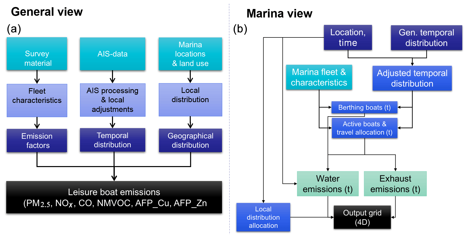
Figure 1 A diagram describing the general modeling approach for the assessment of leisure boat activities and emissions.

The modeling approach in a more detailed overview has been illustrated in Fig. 1b. For each marina location listed, the number of boats and their fleet characteristics are assessed. Throughout the simulation, the date of appearance and departure of each modeled boat in marinas are tracked, which will facilitate more realistic modeling of loads of Cu and Zn from antifouling paints. The temporal profile of leisure boat activities is modeled on an hourly basis, also taking into account the marina location and the estimated boating season length in that location. In particular, for each hour based on the activity profile, boats are split into active and inactive (berthing) boats as in Eqs. (1a)–(1b); the active leisure boats are simulated to operate in the coastal area near the marina, contributing to air emissions according to their fuel consumption, engine properties and emission factors associated with their engine setup (Sect. 2.3).

2.2 Boat characteristics

For the assessment of boat characteristics available information describing the leisure boat fleets for each riparian state of the Baltic Sea was gathered. The most important source for information was survey data and existing reports based on the surveys (Sweden, Swedish Transport Agency, 2010, 2015, Germany, and Denmark), but prior local modeling results (Finland) and port statistics (Baltic states and Denmark) were also utilized. For some riparian states (Poland, Russia) little or no information was available to characterize the national leisure boat fleets.

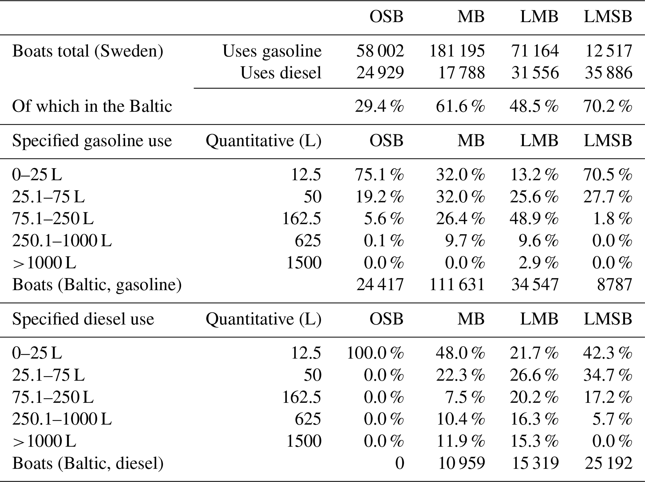
The most detailed information on the characterization of national leisure boat fleet composition by far was available for the Swedish fleet. A detailed questionnaire survey was conducted by the Swedish Transport Agency (2010, 2015). The survey included qualitative information on the activities of 881 000 leisure boats in Sweden, including fleet characteristics, qualitative fuel consumption and travel habits. The Swedish fleet is the largest one in the Baltic Sea and the Swedish coastline covers a large part of the Baltic coastline, ranging from the northern parts of the sea all the way down to the southern parts of the sea. This national study uses a four-tier classification for leisure boats (OSB, MB, LMB and LMSB; for abbreviations, see Table 1) and for each of them there are five possible engine setups, the exception being OSBs which we assume are all gasoline powered. This characterization with 18 different boat bins was also adopted in the BEAM model.

Table 1 Leisure boat classes and assigned attributes based on Swedish survey data (Swedish Transport Agency, 2010, 2015). For different engine setups three values have been specified in the following order: share of engine setup, the average maximum engine power rating and the average engine load.

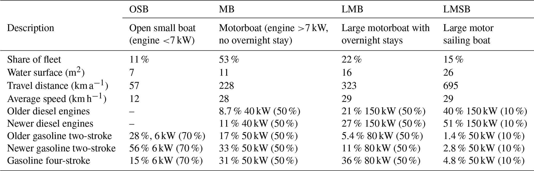
For practical modeling purposes the qualitative survey information on traveling and fuel consumption habits have been converted into quantitative information. As an example, in the questionnaire the number of boats that report traveling 5 to 10 nautical miles per year is available, and we interpret this as meaning that each of these vessels travels 7.5 nautical miles on average (see Appendix B for more information). To obtain average operational speed we have used the survey data that describe the maximum operational speed multiplied with 0.7 (for LMSB this information was not available and the speed value is assumed to equal to the one listed for LMB).

The survey also contains detailed information about engine setups (e.g., stroke type of the engine, fuel type) which was used for all the four leisure boat classes. To calculate the fuel consumption and emissions, assumptions need to be made about the effective engine load factor, i.e., the fraction of installed engine power that is used on average while the boat is moving. There are no data available for this parameter, and as a base case we have used the value in the Guidebook (EEA, 2016) of 50 %. For sailboats we have modified this value to account for the fact that these boats do not use the engine for all travel. Further, for OSB the installed engine power is usually low and used with a slightly higher average engine load factor (we use 70 % instead of 50 %).

The Swedish national survey data also describe some qualitative fuel consumption statistics for the boat categories, but these are not utilized directly in the modeling. Rather, we have used this information to verify that our assumptions on the key factors that define the fuel consumption rates are in agreement with the total fuel consumption statistics derived from the survey data (Appendix B). It should be noted that for most of the riparian states other than Sweden, such a detailed characterization of the leisure boat fleet was not available; therefore the Swedish survey information is widely utilized in this study also for the other riparian states, for which less information is available. The exceptions are for the Danish and German fleet, for which existing information was available for “Share of fleet” in Table 1. A description of the available information on the fleet characteristics for other riparian states is presented in Appendix A.

2.3 Emission factors and fuel consumption

Emission factors and fuel consumption factors are given for in EEA (2016) for different boat types, fuel type (diesel/gasoline), and engine types (two-stroke/four-stroke engines) and emission class (divided into older conventional engines and engines following the 2003/44 EU standard). The boat types in EEA (2016) do not exactly overlap with the boat types used in the Swedish survey, and therefore we have matched these to get usable emission factors (Table 2). It should be noted that the emission factors of Table 2 for two-stroke gasoline engines for CO and NMVOC are very high; for NMVOC the gasoline engines in general have a significantly larger emission factor than the diesel engines. Conversely, the older diesel engines clearly have the highest NO_x emission factors.

Table 2 Specific fuel consumption (SFOC) in grams per kilowatt-hour and emission factors in grams per kilogram of fuel consumed for different boat classes and engine setups. “2S” and “4S” stand for the two-stroke and four-stroke gasoline engines. “_2003” stands for the newer type of engine (older type if not specified). “DSL” stands for diesel engine setups.

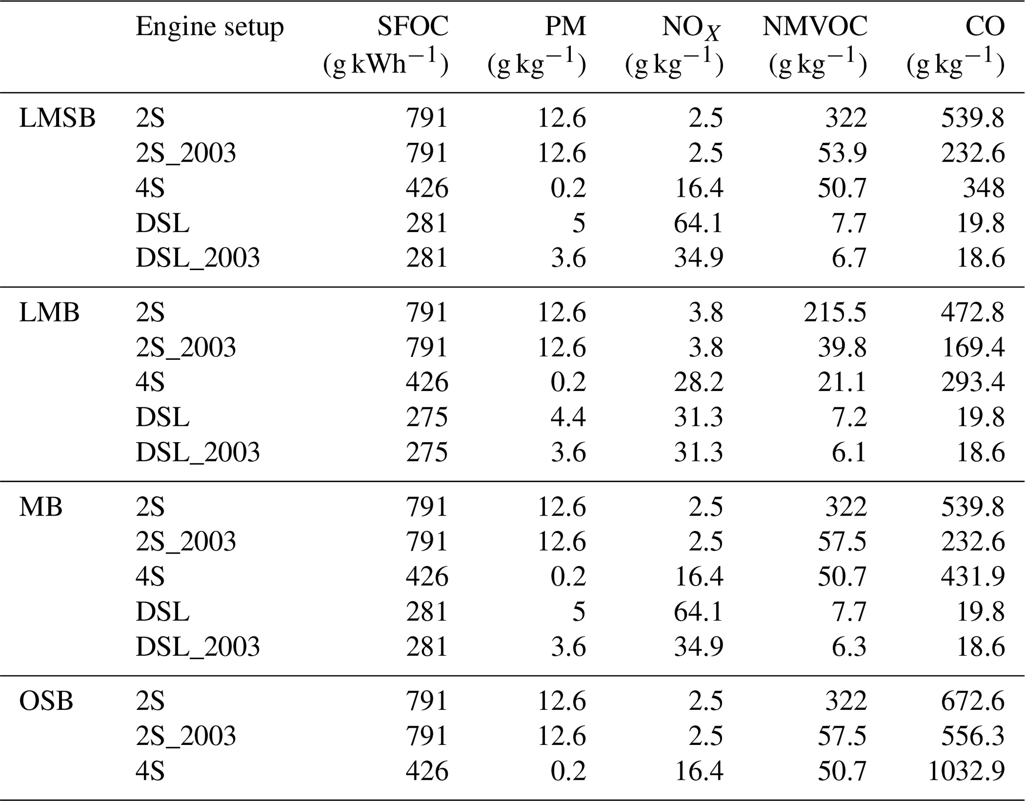
For the modeling of emissions the averaged boat characteristics shown in Table 1 give the average total annual travel distance (D_i) and the average speed for Eqs. (1a)–(1b). For each boat class and engine setup, the unit fuel consumption F_hi can be computed based on Eq. (2b) by combining the data shown in Tables 1 and 2. By combining this information with the emission factors shown in Table 2, the emission can be computed given that the number of active boats is known.

Antifouling

As previously mentioned, the antifouling paint market can differ between and within Baltic Sea states, and Sweden has the most restrictive antifouling legislation. In Sweden, the use of biocidal paints is completely prohibited in the Gulf of Bothnia, and in the Baltic proper (south of Öregrund to Trelleborg) products holding only low (5 %–8 %) Cu₂O are allowed. Only on the Swedish west coast (north of Trelleborg) is the antifouling paint market comparable with the other Baltic Sea states, with authorized paints holding up to 40 % Cu₂O. The release rates of biocides have been shown to be affected by salinity, and a lower release rate is expected in the less saline Baltic Sea as compared to fully marine waters (Ferry and Carritt, 1946; Rascio et al., 1988; Kiil et al., 2002; Adeleye et al., 2016). Recent field studies have also shown a 2-fold increase in copper release rate when five antifouling coatings were exposed in Gothenburg (salinity, PSU, 14) as compared to when exposed in the Stockholm archipelago (salinity 5) (Lagerström et al., 2018).

Table 3 Properties of the antifouling paints assumed to be used in the study. Data were obtained from the Swedish Chemical Agency's pesticide register and from the paints' safety data sheet and technical data sheet.

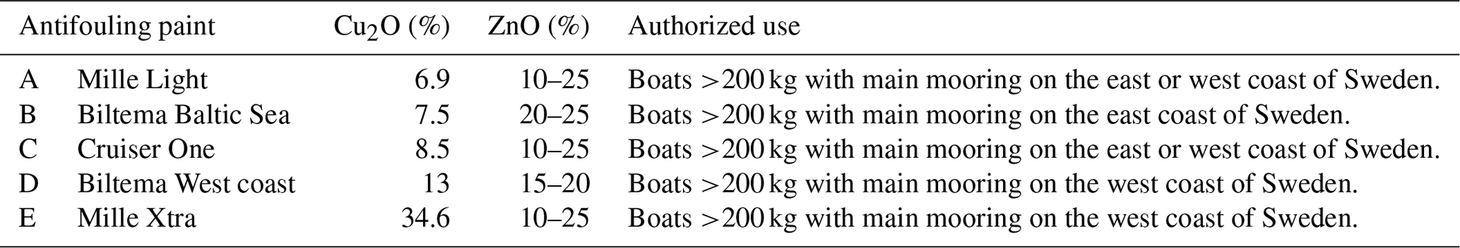
Four different geographical areas (defined in Table 4 and shown in Fig. 6) were designated here to account for the regional differences in the antifouling paint market as well as the impact of salinity on the release rate of Cu and Zn. The release rates of Cu and Zn from five different coatings available on the Swedish market at two salinities (5 and 14) were obtained from Lagerström et al. (2018) as it is the only currently existing study with relevant release rates for the Baltic Sea. As it was not possible to receive boat specific information about antifouling paint use, it was assumed that all boats in the Baltic Sea were painted with one of these five coatings. Hence, the BEAM model does not account for, for example, restricted biocides potentially being released from other coatings. Information about the antifouling paints used in the current study are shown in Table 3. A salinity of either 5 or 14 was assumed for each area to determine release rates of Cu and Zn. The paint use in the “Western Baltic”, “Southern Sweden” and “Northern Sweden” were based on the Swedish regional restrictions (Table 3). For the area “Other”, only paints available on the Finnish market (all but one) were considered. In Lagerström et al. (2018), the release of Cu and Zn was studied over a time period of 84 d at various time intervals (between day 0 and day 7, 14, 28, 56 and 84). Polynomial curves were fitted to the measured cumulative release of Cu and Zn, allowing the modeling of release rates with a daily resolution. For each geographical area, the average daily release rates of Cu and Zn from the paints were calculated (Fig. 2). In Lagerström et al. (2018), the release of Cu and Zn was only studied for up to 84 d. In addition, very thin paint layers were used, which could contribute to uncertainties in the prediction after day 56 at the higher salinity (14) as the measured release could have been affected by the paint becoming depleted in Cu and Zn, resulting in an (erroneous) lower release rate. After day 56, a constant release rate was therefore assumed for all geographic areas to avoid any such potential error.

Table 4 Geographical areas and their assumed antifouling paint use. For each area, the release rates of the paints used were averaged; for example, the release rate for southern Sweden is based on average values from paints A, B and C. The release rate calculations were based on paint-specific release rates from Lagerström et al. (2018) where these were derived from exposure at salinity 5 and 14. The salinity assumption for each area is also listed here.

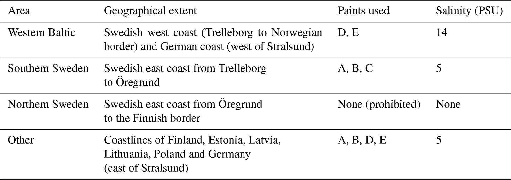
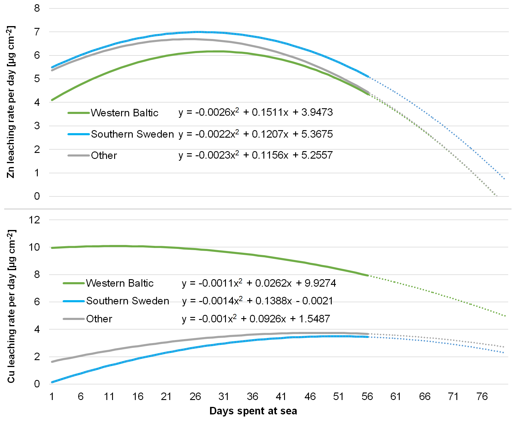
Figure 2 Cu and Zn contaminant leaching rates as a function of days spent in the water (at sea) for different areas of the Baltic Sea, as described in Lagerström et al. (2018).

2.4 Temporal profile of activities

AIS transmitters are mandatory for vessels larger than 300 gross tons (gt). However while leisure boats in general are much smaller than 300 gt, some boat owners (who probably represent a small subset of LMB and LMSB vessel owners) use AIS voluntarily, for example, for safety reasons. As a consequence, while the AIS data cannot facilitate reliable leisure boat modeling with full temporal and spatial coverage by themselves, the data can still be used for the assessment of a generic temporal variation for the activities of leisure boats. In this study we have used the STEAM results based on AIS data for the years 2014–2016 to identify vessels that exhibit leisure boat-like behavior. The AIS data were given by HELCOM, courtesy of the Baltic Sea riparian states. The identification criteria, which were designed based on the survey data for leisure boats, are as follows:

• seasonal activities: the ship must be active only during the ice free season from 1 April to 30 October;

• low annual travel amounts: total travel distance for the ship must not exceed a selected threshold value of 1000 km per year;

• small and non-commercial: the vessel is non-IMO-registered; if the length has been specified in static AIS data, the length must be less than 15 m;

• low utilization: the relative monthly cruising time for the ship must not exceed a selected threshold of 5 %.

Using the selection criteria described above approximately 800–1500 vessels, depending on the year, were identified. It should be noted that the strict identification criteria may filter out some leisure boats; however, the goal is to extract a large representative dataset and not the largest possible dataset; the risk of false positives (non-leisure boat vessel interpreted as one) is significantly reduced and the derived temporal profile does not require all leisure boats to be accounted for.

Using the AIS data from these identified vessels STEAM was used to assess the hourly temporal profile for leisure boat travel distances for the years of 2014, 2015 and 2016. This process has been done by modeling the travel kilometers of the unidentified vessels with STEAM and normalizing the resulting temporal profile to sum up to 1. Also, the three annual profiles were aligned (e.g., so that the days of the week match), averaged and normalized into a single temporal profile, which is presented in Fig. 3.

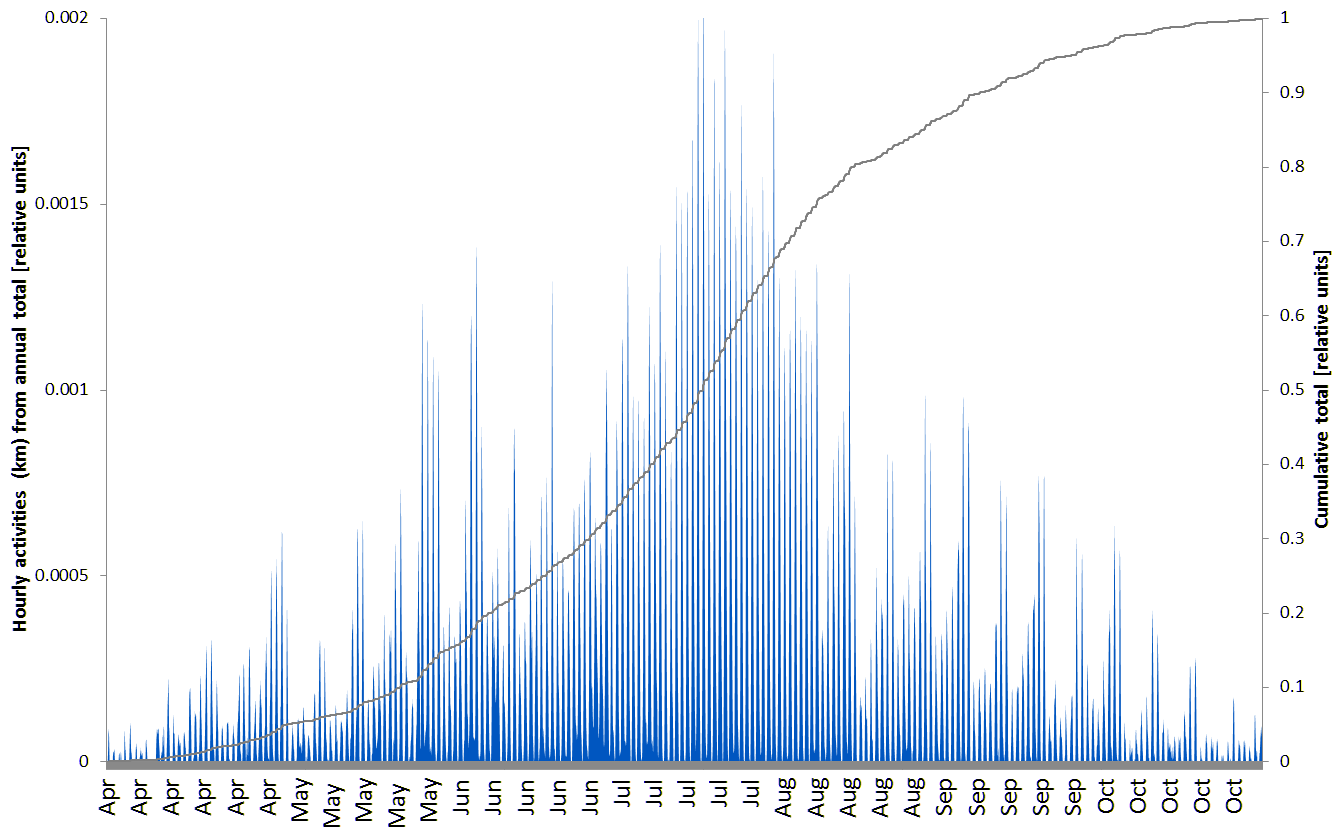
Figure 3 Estimated hourly temporal profile (blue bars) of leisure boat activities in the Baltic Sea based on AIS data and modeled travel distances with STEAM. The secondary vertical axis (right) shows the cumulative temporal profile (gray line) as a function of time.

The Swedish national survey data also describe temporal patterns for leisure boat activities on a monthly basis. In Fig. 4a, a comparison of the derived temporal profile using AIS data is made with the reported monthly profile given by the survey data for all Swedish boats. The survey includes inland use of boats because a distinction was not made between boats along the Baltic Sea coastline and inland water areas. Regardless, the strong correlation of these two suggests that the temporal profile given by AIS data can be used for the assessment of leisure boat activities. In Fig. 4b, it can be seen that the different leisure boat categories exhibit similar temporal patterns throughout the season, based on the survey data. Thus the derived AIS pattern for temporal activities can be applied to each boat category without additional modifications.

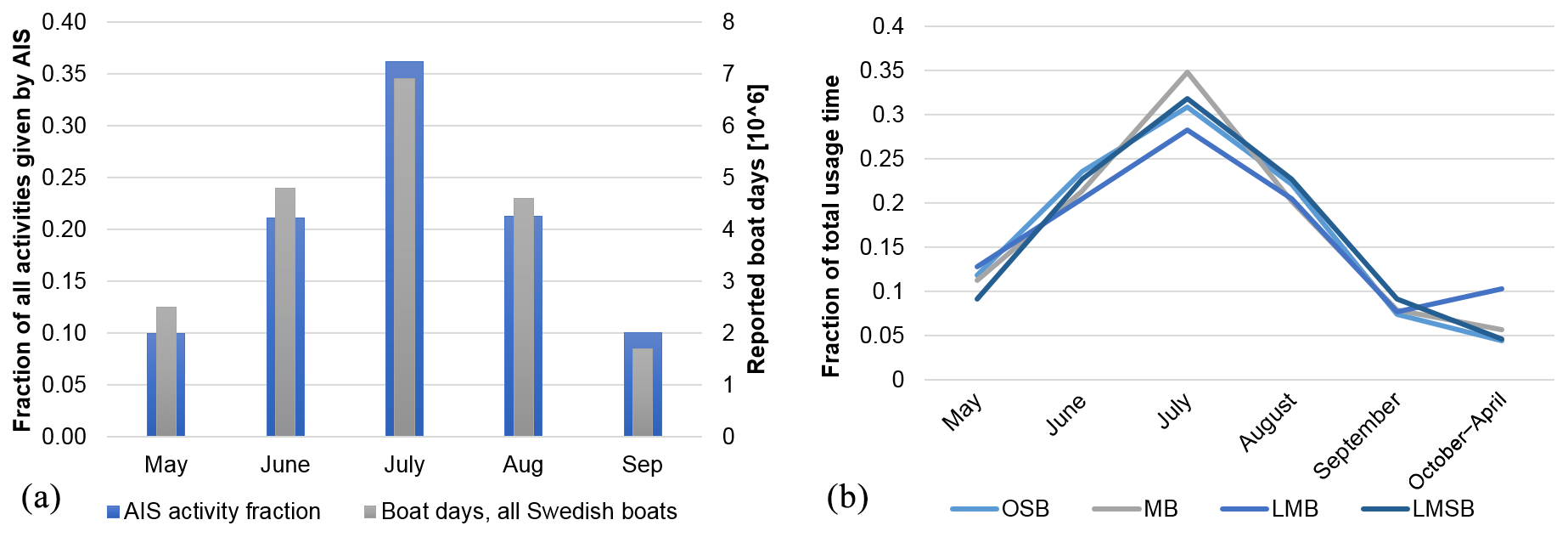
Figure 4 In (a) comparison of the temporal profile given by AIS versus reported boat days for all Swedish leisure boats in 2010. In (b) the reported temporal profiles for each leisure boat class separately are presented based on the reported boat days for all Swedish boats.

Temporal profile adjustment

The temporal profile based on AIS describes the leisure boat activities in the Baltic Sea in general and can be used for the assessment of f(tc) used in Eqs. (1) and (4). However, this temporal profile still lacks the seasonal characteristics that occur for different parts of the Baltic Sea. In the northern parts of the sea the boating season is shorter and starts later during the early summer. In order to take this effect into account, a survey (interviews with marina representatives) was conducted to investigate the temporal patterns of marinas hosting leisure boats at varying latitudes. The survey was conducted by interviewing the marina captains of 11 marinas along the Swedish east and south coastline. The interviews were conducted on the 14 and 16 March 2018. The marina captains were asked to give the number of boats in their marina and assign an approximate percentage of the marina occupancy during the boating season. This included the date when boat owners normally start to launch their boats in spring, dates for which the marina captains could assign the marina occupancy and the date when boat owners normally take their boats from the marina. Instead of using a standardized questionnaire, where the marina captains could assign a specific occupancy to fixed dates, the marina captains were allowed to select dates for which they were confident of giving a good estimate of the occupancy percentage. The survey results are presented in Fig. 5 and locations of corresponding marinas are shown in Fig. 6.

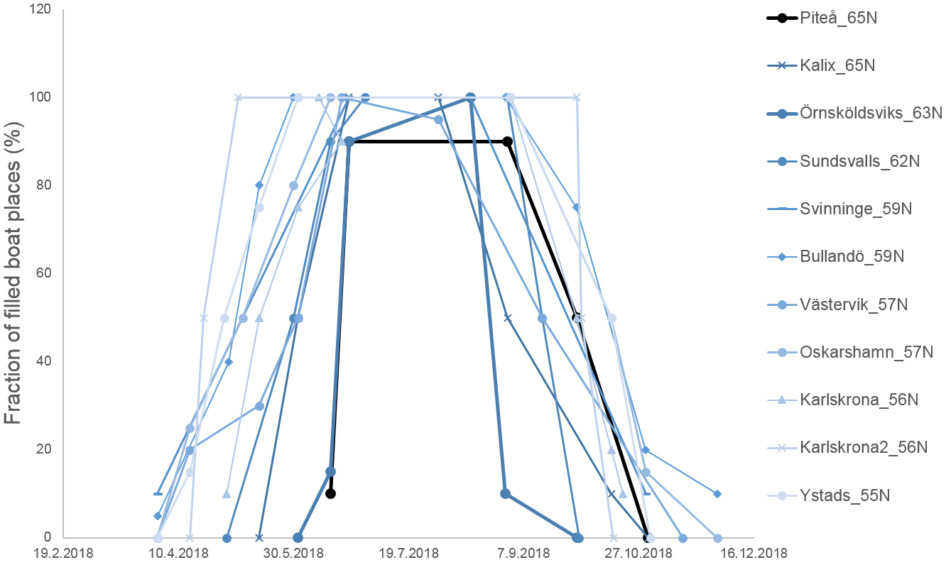
Figure 5 Seasonal patterns based on survey data for selected marinas on the Swedish coast, indicating the utilization rate of marinas as a function of time.

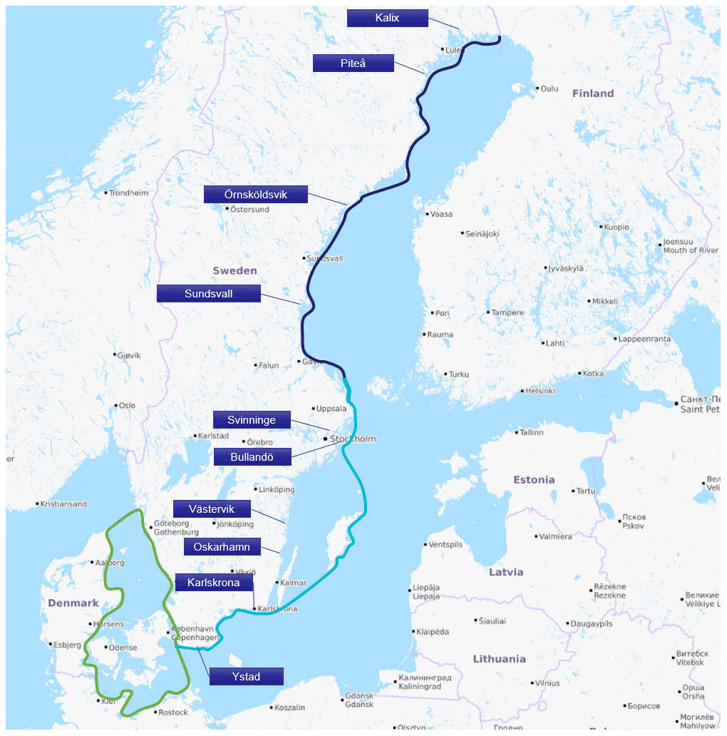
Figure 6 Location of the Swedish boat marinas which were used to determine the boating season length in the Baltic Sea area. Different antifouling paint zones have been illustrated with lines. Dark blue: “Northern Sweden”. Cyan: “Southern Sweden”. Green: “Western Baltic”. Coastal areas for which the AFP zone has not been defined belong to the zone “Other”. Map image provided by © OpenStreetMap contributors 2020, distributed under a Creative Commons BY-SA License.

Based on this survey data a simple statistical model was set up to estimate the season properties, which include the length (L) and the mid-season day (D_M) of the season as a function of latitude coordinate in WGS84 projection (c). In addition, a “ramp-up” (L_U) and “ramp-down” (L_D) length measured in days were also evaluated, which describe the number of days the boat counts increase to 100 % and decreases down to 0 %, respectively. The simple linear statistical model, which is valid in the Baltic Sea only (53^∘ N <c<66^∘ N), is defined as follows:

$$\begin{array}{}\text{(7a)}& {\displaystyle }{D}_{\mathrm{M}}=\mathrm{1.8}c+\mathrm{102},\text{(7b)}& {\displaystyle }L=\mathrm{720}-\mathrm{9.1}c,\text{(7c)}& {\displaystyle }{L}_{\mathrm{U}}=\mathrm{0.2}L,L_{\mathrm{D}}=\mathrm{0.33}L.\end{array}$$

The temporal profile adjustment has the following implications: in the northern marinas the season is shorter and starts later, which will affect the distribution of emissions. Secondly, all activities given by the general temporal profile when no boats are present at the marina are ignored; however we still assume the same amount of total activities regardless of latitude and therefore normalize the marina-specific profile to sum up to 1. According to the survey data and Eq. (7), when the boat season begins ($D_{\mathrm{M}}-L/\mathrm{2}$), the marina capacity utilization reaches 100 % rapidly in 3–4 weeks; when the season ends ($D_{\mathrm{M}}+L/\mathrm{2}$), this utilization rate has decreased to 0 % in 4–6 weeks' time. For a more concrete example, let us consider a marina near Stockholm (c =59.0^∘ N). According to Eq. (7) the length of the season is 180 d, starting around 28 April and ending around the 27 October. The ramp-up number of days is estimated to be 36 d, and therefore by 3 July the marina is expected to have reached 100 % capacity. After the beginning of September the capacity gradually starts to decrease and after approx. 60 d the marina is expected to be empty until the season starts again next year.

2.5 Geographical distribution of boats and activities

The modeled geographical distribution of leisure boat activities is a product of two separate processes: first, the list of marina locations with boat count estimates will outline the general geographical distribution in the Baltic Sea. Secondly, in the vicinity of each marina location the boat activities are allocated at a higher resolution, taking into account land cover information. A list of leisure boat harbors (boat place counts, location) for each riparian state was collected based on survey data, existing national studies and satellite image analysis. The satellite image analysis for marina locations and sizes was performed manually (Fig. 7a). However, for the Swedish coastline a digital mapping of the marinas provided by the Swedish EPA was used that described the geographic areas of the marinas; these areas were converted into boat count estimates, which were manually verified with satellite image analysis.

The full list of marinas includes more than 3000 locations for leisure boats in the Baltic and accounts for more than 250 000 boats in total. Based on the Swedish survey data 37 % of boat owners report using offshore facilities and trailers to harbor their boats. Additionally, a significant fraction of the boats are located on private shores outside of marinas. To take this into account in the modeling we assume that the listed marina locations are expected to harbor only 50 % of the total fleet, and we therefore multiply each marina boat count with a factor of 2; in other words, we assume that for each boat in a marina there is another boat not accounted for and its activities can be associated with the area near the marina location. This assumption is consistent, for example with the estimates of Daehne et al. (2017), who report 43 000 German boats for the Baltic Sea coastline. Our boat count based on satellite images yields 19 900 boats for the German Baltic Sea area, but it becomes consistent with the Daehne et al. (2017) estimate if offshore locations are considered.

In Table 5 the number of boats in marinas, on private shores and at offshore facilities for all riparian states are shown. The fleet composition is also shown in the table, which has been assessed based on survey data. For the Finnish fleet it should be noted that the total surveyed boat count (195 000) is for fuel-consuming boats without distinction between the Baltic Sea and inland waters. In another study by the Finnish authorities¹ it has been estimated that there are over 90 000 boats on the Finnish coast, which is consistent with our estimates based on satellite analysis – once the multiplication with a factor of 2 is done.

Table 5 National leisure boat counts based on survey data (Appendix A) and coastal satellite image analysis. Total modeled number of boats equals the preliminary boat count (marina) added with the estimates for boats on private shores and in trailers. The fleet composition described corresponds to the percentages used for OSB, MB, LMB and LMSB types, in the given order summing to 100 %.

Local geographical distribution

The Swedish surveys (Swedish Transport Agency, 2010, 2015) indicate that the clear majority of leisure boats regardless of type operate very locally near their marinas. Based on this information it is sufficient for the scope of this study to allocate all leisure boat activities to the vicinity of marinas, although some marina-to-marina activities for the larger boat classes will be mis-allocated in this estimation. The overall process of analyzing the coastline for marina locations with boat counts and deriving local distributions of activities is described in Fig. 7.

For each marina we form a list of local discrete locations for possible boating activities defined with a selected resolution of 0.2 km × 0.2 km. The maximum range for this mapping has been set to (50 km) and land-use data have been used to omit all discrete locations that are not located in the Baltic Sea. For each of these locations the distances to the marina (r_m) and to the nearest coastline (r_c) are evaluated. For r_c in particular, land-use information (OpenStreetMap) has been used in the assessment, also taking into account islands.

For each listed discrete location for possible boating activities, we compute an activity probability p(r_mr_c). In this study we have opted for a simple exponential function to express p(r_mr_c), given by

$$\begin{array}{}\text{(8)}& p\left(r_{\mathrm{m}}{r}_{\mathrm{c}}\right)=e^{-a\left(r_{\mathrm{m}}+b{r}_{\mathrm{c}}\right)},\end{array}$$

where the term r_m+br_c can be regarded as the “effective” distance from the marina that also considers the distance to the nearest coastline, and the factor a defines how strongly the probability decreases as a function of this distance. Presumably the factors a and b depend on the leisure boat class; for example, the larger boats are used for longer travel and can safely be operated farther away from the coastline. However, due to lack of usable data we have settled for generalized empirical values for a and b that are the same for each boat class.  Finally we normalize the probabilities so that they sum up to 1.

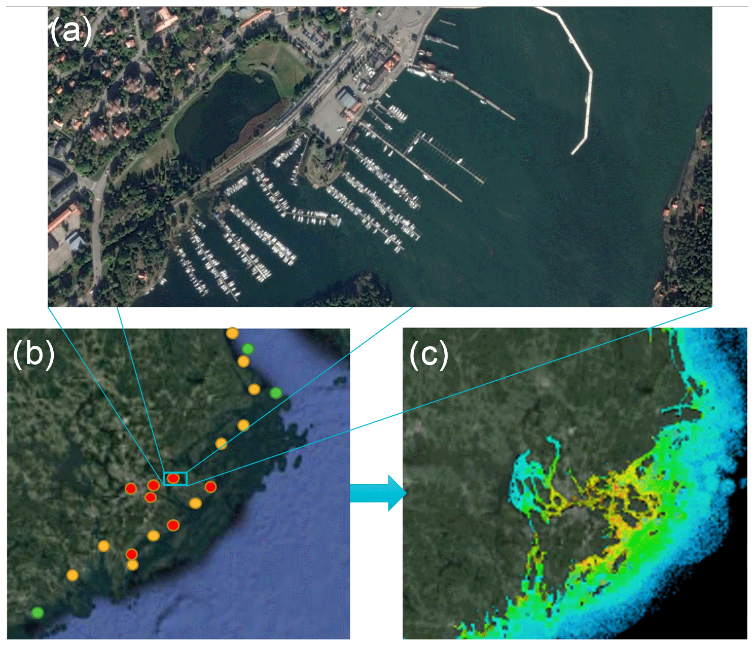
Figure 7 The overall process for geographical distribution of activities. In (a), an example of satellite imagery used to calculate the number of boat places in a small boat marina (58.9^∘ N, 17.95^∘ E; Sweden). In (b) the analysis for boat counts and marina locations has been applied for a selected region. In (c) an example is given when emissions of selected marinas are allocated according to Eq. (8). Satellite image background provided by © Google Earth.

In the study by Montes et al. (2018) the distribution and intensity of recreational boating in the southeast US has been presented. The findings of the study performed in Florida are not fully applicable to leisure boats in the Baltic; however, the observed boating patterns do exhibit clear dependencies on both the coastline distance and the marina distance. Due to the lack of data we assume the effects of r_m and r_c to be equal and set the value for b as 1 and use a value of 0.2 for a, which we estimate to lead to similar distributions as were obtained with the generalized additive model (GAM) in Montes et al. (2018).

3 Results

The BEAM model was used to estimate the hourly emissions of leisure boats in the Baltic Sea starting from 1 March until the end of November. It should be noted that in the production of input datasets a heterogeneous collection of survey material, AIS data and satellite imagery was utilized dating to between 2010 and 2017. Therefore the presented results do not represent any specific year in particular. The modeled annual total emissions, fuel consumption and travel amounts are presented in Table 6.

Table 6 Modeled leisure boat fuel consumption, emissions and travel distances in the Baltic Sea, for different flag states and boat types. Flag state category “Other” includes Russia, Estonia, Latvia, Lithuania and Poland.

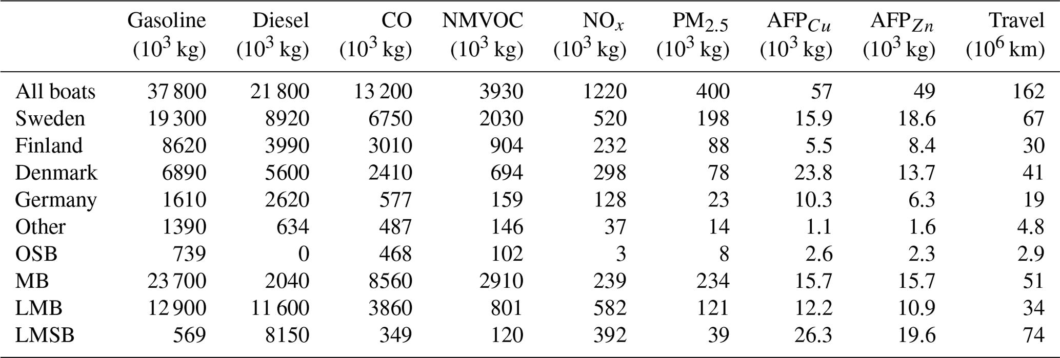
According to the results, almost half of the gasoline fuel consumption, CO-, NMVOC- and PM_2.5 emissions comes from the Swedish leisure boat fleet. For exhaust emissions and fuel consumptions Denmark and Finland have the second and third largest contribution, in changing order depending on the pollutant type; Germany has the fourth largest contribution for these estimates. Together these four flag states contribute 96 %–99 % of exhaust emissions from all leisure boats in the Baltic Sea. The combined fuel consumption is estimated to be approximately 60 ×10⁶ kg of which the clear majority is gasoline fuel.

Quantitative estimates for Swedish leisure boat fuel consumption for all boat classes can be derived from the Swedish leisure boat survey. Based on these survey material estimates, the modeled fuel consumption for both gasoline and diesel are in fair agreement with modeled values (Appendix B). This agreement gives an indication that the average speeds, engine loads and engine power ratings used can be considered realistic at least for the Swedish fleet. Emissions of NO_X, PM_2.5 and CO for the whole Swedish leisure boat fleet (also comprising boats in inland waters) have been determined by the Swedish EPA for the year 2018 and were 1273 t (NO_x), 148 t (PM_2.5), 2744 t (NMVOC) and 18 854 t (CO) (Swedish EPA, 2018). Based on the Swedish survey data, a clear majority of MB and LMSB boats and half of the LMB boats operate in the Baltic Sea for the Swedish fleet; based on this, the emission totals given by Swedish EPA seem higher for NO_x and CO while PM_2.5 is lower than the presented BEAM predictions would suggest.

The boat class-specific emission totals shown in Table 6 show that the MBs are responsible for 74 % of released NMVOC emissions, mainly due to high amount of gasoline used with old two-stroke gasoline engines. The motorboats are also modeled to be responsible for 65 % of CO emissions and 58 % of PM_2.5 emissions. Together, LMB and LMSB release 80 % of NO_x emissions due to the higher use of diesel fuel. For all modeled emission types the smallest boat category OSB has very low shares in general.

The loads of Cu and Zn from antifouling paint are affected by sea salinity as well as the types of paint allowed and used in the different parts of the Baltic Sea. As a consequence, 58 % of the Cu emissions and 42 % of Zn originate from the relatively short combined coastline of Denmark and Germany due to the combination of the higher ambient salinity (resulting in higher leaching rates) and types of paints allowed. In contrast, the much longer combined coastline of Finland, Russia, the Baltic States and Poland produces only 11 % of Cu and 20 % of Zn emissions. For antifouling paint contaminants the contribution from LMSB boats is the largest (26.3 t), due to the large water surface area (26 m²) for this boat type.

Figure 8 Estimated geographical distribution of NMVOC exhaust emissions and the copper emissions from antifouling paints for a selected area. Satellite image background provided by © Google Earth.

In Fig. 8 the estimated NMVOC emissions are presented. It can be seen from the figure that there are several hotspots, including the archipelago near Stockholm, Helsinki area, Copenhagen, Gothenburg and the Lübeck area. It should be noted that the modeled geographic distribution of emissions on a local level is only indicative due to the lack of usable data to parametrize Eq. (8). The copper emission from antifouling paints is also presented in the figure (upper left) for the southwestern part of the Baltic Sea, and in contrast with NMVOC, the copper emissions are heavily concentrated on marina locations. The reason for this is that all boat classes are expected to have a very low number of active hours per year, which in turn causes the main source of releases to be stationary boats at the marina locations. As an example, consider OSBs that have an average annual travel amount of only 57 km, which is reached with less than 5 h of activity during the year.

The geographical distribution of exhaust emissions is difficult to predict due to the lack of activity data available for leisure boats. As was discussed in Sect. 2.4 we used AIS data for 2014–2016 and STEAM to isolate a small subset of leisure boats, which was used to assess the temporal distribution of activities. Presumably, this set of boats is a subset of the larger boat classes (LMB, LMSB), and the geographical distribution of modeled fuel consumption for these boats should be comparable to BEAM predictions for the largest boat classes. We used these AIS data to model the fuel consumption of these small number of boats for 2014–2016, and the averaged results of this modeling are presented in Fig. 9. For comparison, the BEAM modeled fuel consumption for LMSBs is presented in the figure. To be able to compare these modeled distributions, the modeling resolution has been set to be identical and the grid cell values have been scaled to be in proportion to the average grid cell content. It can be seen from the figure that the AIS-driven approach shows marina-to-marina boat activities which have not been considered in BEAM. In both approaches the clear majority of activities (traveling amount and thereby fuel consumption) coincide near coastal areas and are heavily concentrated on the same hotspots – the area near Lübeck being an exception.

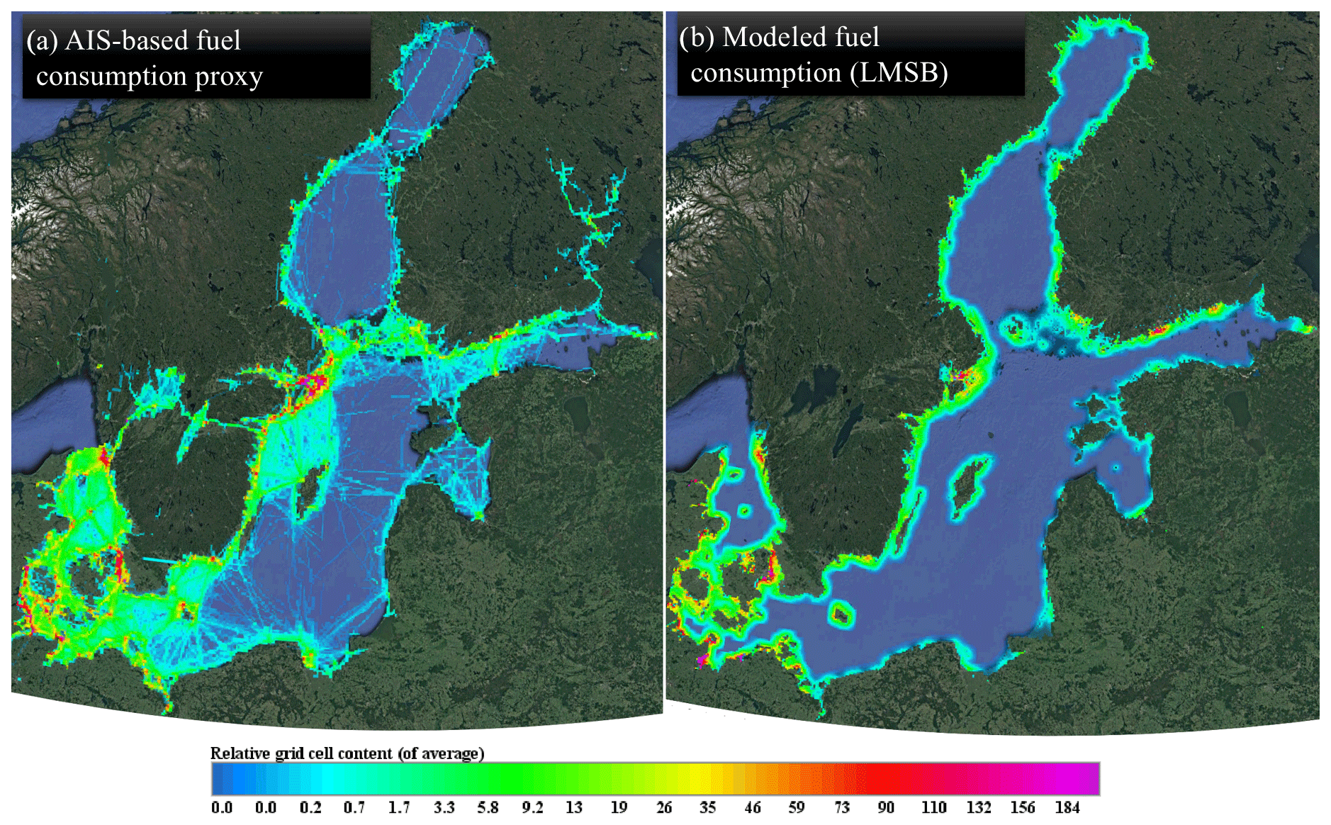
Figure 9 Estimated distribution of leisure boat fuel consumption in terms of grid cell average. In (a) the predictions based on AIS (STEAM) are shown. In (b) BEAM predictions for LMSB fuel consumption is shown. Satellite image background provided by © Google Earth.

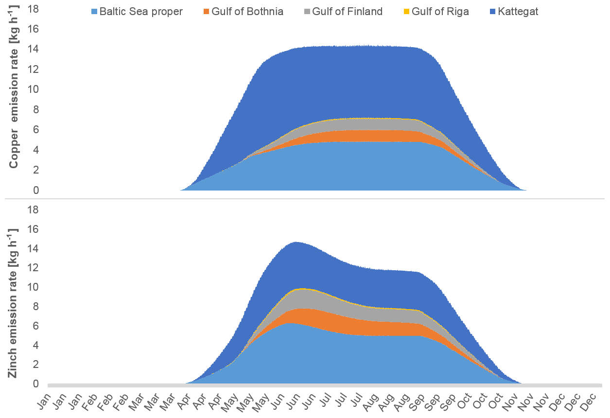
Figure 10 Modeled antifouling paint contaminant leaching rates for different parts of the Baltic Sea.

The modeled emissions have a clear seasonal patterns, and this is especially evident for the modeled antifouling paints. The hourly emission rates for copper and zinc contaminant are presented in Fig. 10 for different parts of the Baltic Sea. As can be seen from the figure, copper and zinc emissions have different temporal patterns which are caused by the dynamic emission factors shown in Fig. 2 (Lagerström et al., 2018). According to the model, the total zinc emission release rate peaks at the beginning of June, whereas the releases of copper are more evenly distributed during the season. The two dominant regions for copper and zinc emissions are clearly the Kattegat and the Baltic Sea proper.

Leisure boat emissions versus commercial shipping

The emissions and impacts of registered shipping in the Baltic have been studied thoroughly, and these known emissions have been compared against the leisure boat emissions to gain a better perspective on the presented total emissions. In Fig. 11, the total emissions of registered shipping in 2014 using STEAM are presented. For commercial shipping, the activities and emissions are somewhat evenly distributed during the year, whereas leisure boat emissions are heavily concentrated in the summer months. To highlight this contrast, the leisure boat emissions have also been compared against the commercial emissions in July.

From this annual comparison it can be seen that while the total travel kilometers of leisure boats are comparable to the total of the registered fleet, the fuel consumption, NO_x and PM_2.5 are significantly lower (1.2 %, 0.4 % and 2.7 %, respectively) for leisure boats. However, the zinc contaminants from the antifouling paints and CO are lower but comparable to those of the registered fleet, and copper contaminants are 19 % of the respective total. The higher loads of copper and zinc from the commercial fleet can primarily be explained by legislation and use patterns. Paints for commercial ships are allowed to have a higher release rate of copper and zinc as compared to paints for the leisure boat market, and the leisure boats are assumed to be used during April to October only. Since NMVOC emission factors for leisure boat engines are 1–2 orders of magnitude larger than for the large well-optimized marine diesel engines, the NMVOC emissions from the leisure boats are estimated to be significantly larger than the emissions from registered vessels. In July the relative importance of leisure boat emissions with respect to the commercial fleet is greatly emphasized in this comparison. In particular NMVOCs are 500 % larger, CO emissions are 140 % larger and zinc emissions are 80 % larger for leisure boats than the emissions from registered traffic during July. It should also be noted that the emissions released by leisure boats are heavily concentrated near populated coastal areas, of which Fig. 8 gives an indication.

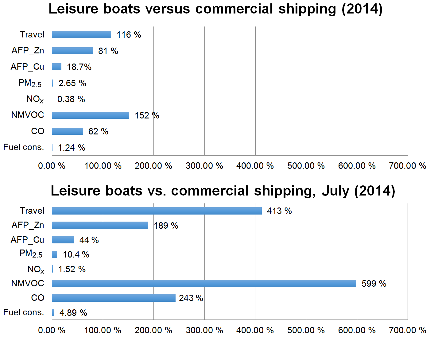
Figure 11 Modeled leisure boat emissions, fuel consumption (kg) and travel kilometers with respect to those of the commercial fleet in 2014 and separately for July 2014. A value of 100 % indicates an equal contribution from small boats and commercial shipping.

4 Conclusions

A new simulation model for the assessment of leisure boat activities and emissions in the Baltic Sea (BEAM) has been presented. In the model both the temporal and spatial distribution of emissions is considered and leisure boat fleet characteristics can be customized, for example, according to available survey material. For this study in the Baltic Sea we have utilized a wide range of information sources and data processing techniques in our modeling, including AIS data, coastline satellite imagery, survey material, data on marina locations with boat counts and land-use information.

The leisure boat emissions have previously been largely unknown in the Baltic Sea, and the results given by the presented model improve this situation. Leisure boat emissions, being heavily concentrated on the populated urban areas during the summer months, are rarely used – and most often neglected - in dispersion modeling or other impact assessment modeling work such as marine ecosystem modeling (e.g., Raudsepp et al., 2019). The presented model can be used to produce dynamic emission datasets for selected exhaust pollutants and water contaminants, which could be utilized in the abovementioned studies in the future.

According to our results some of the pollutants emitted by leisure boats are very substantial when compared against the emissions originating from registered, commercial shipping activities in the Baltic Sea. This comparison has been made based on modeled shipping emissions for 2014; however, it should be noted that the modeled emissions are fairly similar for other years during 2012–2018 given by STEAM. CO emissions equal 70 % of the registered shipping emissions and NMVOC emissions equal 160 % with respect to commercial shipping. However, modeled NO_x and PM_2.5 from leisure boats are clearly less significant with respect to the registered shipping emissions. In absolute terms the modeled emissions are 13 000 t for CO, 3900 t for NMVOC, 400 t for PM_2.5, 1200 t for NO_x, and 57 t for copper and 49 t for zinc water contaminants. It should be noted that most of the modeled emissions occur during the summer months, during which their relevance for nearby marina areas is further increased. Given the relatively large emission estimates for leisure boats, especially for NMVOC, this commonly overlooked source of emissions deserves to be further investigated in greater detail. Also, the impact on air quality should be studied further with measurements and dispersion modeling. It should be noted that while the leisure boat emissions are significant with respect the commercial fleet, the modeled exhaust emissions are still fairly small when compared against, for example, national total anthropogenic emissions. For example, the NMVOC emissions for Finland are reported² to be 88 t in 2016.

Clear majority of the emissions can be attributed to Swedish, Finnish and Danish boats, of which the main contribution originates from motor boats (MB, LMB), but the leisure boat fleets have the potential to become larger in Russia, Estonia, Latvia, Lithuania and Poland in the future. The motorboats are especially dominant in the emissions of NMVOC and CO, largely due to the large number of motorboats with old two-stroke gasoline engines. Therefore, an effective approach to reduce leisure boat impacts on marina areas could be to reduce the number of these engine setups; however, a more thorough impact analysis should be conducted first. As older engines are replaced by newer combustion engines or electrical engines the situation will naturally improve. For antifouling paint leach, the largest boat category has the highest impact. The smallest contribution in terms of exhaust and water emissions comes from the smallest boat type, OSB.

The uncertainty margin for the presented results is fairly high, which should be narrowed down with further development and research. The most notable sources for error in this study are arguably the national total boat counts. The satellite analysis used is difficult to conduct and is subject to interpretation. Also, the boats on private shores and the use of offshore trailers is a matter of concern for the modeling, and the survey material gives only an indication of the number of boats that are outside marinas. As a second source of error, the fleet composition and the split of engine setups are difficult to customize for other riparian states of the Baltic Sea besides Sweden, which has by far the highest-quality survey material available. Third, the emission factors used for different engines are based on averaged Swedish data compiled over several years, which introduces uncertainties. The fourth source of error is that our treatment of temporal and spatial patterns for boats does not consider the different boat classes independently, but a generalized profile is used. Finally, the geographical distribution of activities on a local scale is based on a model that was set up with a very low number of evaluation data, and marina-to-marina activities could not be considered. Arguably the highest confidence can be given to the temporal profile of activities based on AIS data analysis. Even for the temporal profile, further model development is required so that a specific year can be targeted and, for example, the impact of weather can be taken into account.

Appendix A: Fleet description for riparian states other than Sweden

A1 Fleet characteristics for Finland

A study commissioned by the Finnish Maritime Administration and conducted by VTT (Technical Research Centre of Finland) (Räsänen et al., 2005) concluded that in Finland, there were about 390 000 small boats with a motor. The national small boat registry (Finnish Transport and Communications Agency Traficom, 2015) lists over 195 000 small boats powered by an engine, which is about half of the previous assessment. The discrepancy in boat numbers may be partly due to the new boat registry requiring an active registration of all boats with an engine. If a boat is not actively used, it may not be included in the small boat registry. The information contained in the small boat registry is only an indication of the total fleet of boats because it does not distinguish between boats used on the Baltic Sea coastline and those used in inland waters. For this reason, the satellite imagery from the Finnish coastline was searched for small boat marina locations. Vessel counting was done based on available places for boats, not the actual boats themselves, because it was likely that some of the boats were in use during the time satellite image was taken. On the other hand, counting the boat places automatically assumes 100 % use of available capacity. Regardless, 475 boat marinas were found in the Finnish coastline, the Turku archipelago area and Ahvenanmaa islands. These marinas had space for over 50 600 vessels. The vessel characteristics for the Finnish fleet are based on the Swedish survey. No official records exist for fuel sold to small boats in Finland.

A2 Fleet characteristics for Denmark

The Danish Maritime Authority registers leisure boats over 20 gt (type of boat, type of propellant or home port is not available), but no register of all Danish leisure boats was seen to be available. Based on the information found at https://www.sailbuddy.com/map (last access: 17 September 2020) it was possible to locate 338 marinas in the Danish part of the Baltic Sea. This information included the geo-reference of the marina, the number of mooring places and contact details for further contact to individual harbors. The largest of the harbors were contacted by telephone and email to inquire whether the marina had a separate fuel station, so that an estimation of fuel consumption could be made. Fifteen of the biggest marinas fit the conditions and were able to provide information on the fuel consumption in their marina, although the fuel consumption statistics were not ultimately utilized in this study. It was estimated that the listed marinas had space for over 59 600 vessels according to satellite image analysis. The fleet composition was observed to be different to the one reported for the Swedish fleet.

A3 Fleet characteristics for Germany

A telephone survey formed the basis of the bottom–up statistic, which was used to obtain information on the annual fuel sales in liters (diesel and petrol) from the German water petrol stations in the Baltic Sea. All 39 petrol stations on the German Baltic Sea coast were contacted and information from 35 stations was received and recorded.  Research was conducted prior to the survey on the number of water petrol stations and their connected berth.

The number of berths is relevant to the research, since the study examined whether the revenue per berth is similar in different regions on the German Baltic Sea coast and can therefore be transferred to other regions. Since there are no exact statistics on how many German leisure boats exist in the Baltic Sea, this study relates to a previous study which equates the number of berths to the number of existing vessels.

An online questionnaire formed the basis of the top–down statistics. The survey was conducted by 265 German leisure boat owners who sail the Baltic Sea. The survey asked technical questions regarding the characteristics of their vessel, such as motor and fuel consumption, as well as information on their activities. Activities were divided into two categories: popular short trips and popular long trips. The boats in the survey were classified into three sub-types: sailing boats with engines, sailing boats without engines and motorboats.

It was estimated that the listed marinas had space for approx. 20 000 vessels according to satellite image analysis, which was approximately half of the number of vessels according to survey material. The fleet composition was observed to be different than the one reported for the Swedish fleet.

A4 Fleet characteristics for Poland, the Baltic states and Russia

Local authorities were contacted for existing inventories and surveys for leisure boat activities. Unfortunately, inventories were not available, and leisure boat activity in the Baltic Sea for Poland, Lithuania, Latvia, Estonia and Russia were estimated based on marina locations (listed port areas, satellite images) and supporting information. The mix of gasoline and diesel use was taken from the Swedish survey data.

Small harbors along the eastern coast of the Baltic Sea were positioned based on reference locations in http://en.seaclub.lv/ports/estonia/ (last access: 17 September 2020), and their size was estimated by satellite images. The total number of crafts for Estonian leisure boats was estimated to be 1075, which compares well to the national registry database (700 yachts + small ships which include 134 motorboats and 206 work boats).

Appendix B: Fuel consumption estimates for the Swedish fleet and survey data processing

A large part of the fleet characteristics used originate from the Swedish survey studies (2015), such as the average travel distances and fractions for different engine setups. The survey data are by their nature qualitative and do not easily provide quantitative information. To overcome this, the survey data have been processed so that they are more usable for the modeling.

The first step in this process was the removal of “blank” answers such as (“Not sure”), which were selected by the users quite often. We simply assumed that the users with blank answers would follow the same distribution as the other users did with their answers. In other words, we scale the number of non-blank answers so that in total they sum up to 100 % of all questionnaire users. Such a blank-removed questionnaire summary for fuel consumption habits has been shown in Table B1.

We transform the qualitative answer possibilities (e.g., 0–25 L) into quantitative ones using the average value of the specified range (e.g., 12.5 L). For the last fuel consumption range (>1000 L) the averaging is not possible, and we have assumed a value of 1500 L as the quantitative value. For other statistics such as travel distances we have assumed a 150 % value for the last answer option if the range has been left open in a similar fashion.

Based on the survey material the total number of gasoline and diesel boats have been specified for each boat class. In addition, the fraction of boats in the Baltic Sea has also been specified, which in turn yields the number of gasoline- and diesel-powered boats in the Baltic. Finally, the total fuel consumption estimates for each boat class can be computed by combining (a) the boat counts, (b) the quantitative fuel consumption thresholds and (c) the distribution of boat owner answers. These totals are shown in Fig. B1, and for comparison the BEAM model predictions are also shown in the figure. For the comparison, the fuel consumption totals are presented in metric tons (t), which we have obtained from the quantities in liters by using a density of 0.8 kg L⁻¹ for both diesel and gasoline.

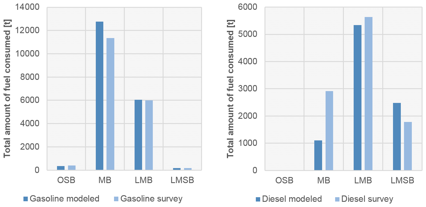
Figure B1 Comparison of fuel consumption statistics for the Swedish fleet in the Baltic Sea against BEAM model predictions. Comparison has been made for each class and separately for gasoline and diesel setups.

Table B1 Swedish leisure boat survey material (fuel consumption and boat counts) and derivatives processed based on the data. ”L” corresponds to liter.