the Creative Commons Attribution 4.0 License.
the Creative Commons Attribution 4.0 License.
 | 22 Sep 2020
Response of near-inertial energy to a supercritical tropical cyclone and jet in the South China Sea: modelling study
Hiu Suet Kung
We used a well-validated three-dimensional ocean model to investigate the process of energetic response of near-inertial oscillations (NIOs) to a tropical cyclone (TC) and strong background jet in the South China Sea (SCS). We found that the NIO and near-inertial kinetic energy (KEni) varied distinctly during different stages of the TC forcing, and the horizontal and vertical transport of KEni was largely modulated by the velocity and vorticity of the jet. The KEni reached its peak value within the inertial period after the initial TC forcing stage in the upper layer, decayed quickly by 1∕2 in the next 2 d, and further decreased at a slower rate during the relaxation stage of the TC forcing. Analyses of the KEni balance indicate that the weakened KEni in the upper layer during the forcing stage was mainly attributed to the downward KEni transport due to pressure work through the vertical displacement of isopycnal surfaces, while upward KEni advection from depths also contributed to the weakening in the TC-induced upwelling region. In contrast, during the relaxation stage as the TC moved away, the effect of vertical advection on KEni reduction was negligible and the KEni was chiefly removed by the outward propagation of inertial-gravity waves, horizontal advection, and viscous dissipation. Both the outward wave propagation and horizontal advection by the jet provided the KEni source in the far field. During both stages, the negative geostrophic vorticity south of the jet facilitated the vertical propagation of inertial-gravity waves.
- Article
(14131 KB) - Full-text XML
- BibTeX
- EndNote


Near-inertial oscillations (NIOs), whose frequencies are close to the local inertial frequency, contain around half of the observed internal wave kinetic energy in the ocean (Simmons and Alford, 2012). NIOs also greatly affect the kinetic energy budget in the deeper ocean as they propagate downward from the surface and enhance the mixing by increasing vertical shear (Gill, 1984; Gregg et al., 1986; Ferrari and Wunsch, 2009; Alford et al., 2016).
Tropical cyclones (TCs), with the rapid change of wind stress, provide an important generation mechanism for the NIOs. Observational studies related to a single storm or tropical cyclone (Price, 1981; Shay and Elsberry, 1987; D'Asaro et al., 1995) showed that the NIOs related to TCs can be a factor 2–3 larger than the background NIOs and last for more than five inertial periods (IPs). Using a hurricane–ocean coupled model, Liu et al. (2008) estimated that the energy input of tropical cyclones into the near-inertial currents was about 0.03 TW, about 10 % of the total wind-induced near-inertial energy (Watanabe and Hibiya, 2002; Alford, 2003). The input of wind energy to the near-inertial band is also controlled by the translation speed of the TC (Uh) (Geisler, 1970; Price, 1981). In fact, the NIOs are largely variable during the forcing and relaxation stage of the TC forcing related to the intensity and translation speed of the TC. The variation is determined not only by the different magnitude of the input of wind energy but also by the different dynamic conditions that regulate the near-inertial kinetic energy (KEni) transport during these stages. The variable response of NIOs during different stages of TC forcing is critical for understanding the process and physics of NIOs.
Once generated, the characteristics of NIOs, in terms of the decay timescale, propagation direction, and propagation speed are influenced by various mechanisms. In linear wave theory, the β effect leads to equatorward propagation of the NIOs, and their decay timescale is reduced because of the vertical propagation into deeper ocean (Gill, 1984; D'Asaro, 1989; Garrett, 2001). Background flow fields also have great influence on the evolution of NIOs. The influence of background vorticity on NIOs has been observed by Weller (1982) and Kunze and Sanford (1984) and proven analytically by Kunze (1985), Young and Jelloul (1997), and Danioux et al. (2015). A numerical study using a primitive equation model with a turbulent mesoscale eddy field and uniform wind forcing came to a similar conclusion (Danioux et al., 2008). Non-linear interactions also provide a mechanism for increasing the vertical wave number and thus for larger vertical shear and dissipation and reduced decay time (Davies and Xing, 2002; Zedler, 2009). In addition to modifying the characteristics of the inertial-gravity waves, nonlinear advection related to a front can transport NIOs away from the storm track and to higher latitudes (Zhai et al., 2004). Recent observations and numerical studies in the Gulf Stream, Kuroshio, and Japan Sea revealed the role of vertical circulation on the generation and radiation of near-inertial energy (Whitt and Thomas, 2013; Nagai et al., 2015; Rocha et al., 2018; Thomas, 2019).
The South China Sea (SCS) is a region with frequent tropical cyclone occurrence: ∼10 each year (Wang et al., 2007). Observations (Sun et al., 2011a, b; Xu et al., 2013) and numerical studies (Chu et al., 2000) indicated that these TC events are sources for near-inertial energy bursts. Additionally, the SCS circulation contains abundant energetic flow (e.g. Qu, 2000; Gan et al., 2006; Gan et al., 2016a) and mesoscale features, such as a strong coastal jet off the Vietnamese coast (e.g. Gan and Qu, 2008) and eddies (e.g. Chen et al., 2012). The distribution and evolution of the TC-induced NIOs are susceptible to the influence of these background currents. (Sun et al., 2011a, b). However, the estimate of the total contribution of a TC to the KEni in the SCS is difficult to obtain from observations or linear wave theory due to sparse spatial observations and the non-homogenous nature of SCS circulation.
In this study, we apply a well-validated numerical model with specific China Sea configurations to examine the response of KEni to a large TC and background jet over the sloping topography in the SCS. A description of Typhoon Neoguri and the details of the numerical model implementation are given in Sect. 2. In Sect. 3, the general characteristic response of the near-inertial current and the energy fluxes during the TC forced stage and their later relaxation stage as TC moved away from the concerned region are presented. Following Sect. 3, the KEni equation is used to identify the dynamic processes of the vertical viscous dissipation, pressure work, and nonlinearity during different phases of the NIOs.
2.1 Typhoon Neoguri (2008)
Typhoon Neoguri formed east of the Philippines and entered the SCS on 15 April. It first moved west–northwest with an average translation speed of 5.8 m s−1 before it slowed down to 1.6 m s−1 on 16 April, based on the Joint Typhoon Warning Center (JTWC) best track data, (Fig. 1). On 17 April, Neoguri sped up to 3.8 m s−1, turned more northward, and developed into a typhoon with a maximum wind speed of 51 m s−1 and an MSLP (minimum sea level pressure) of 948 hPa, at 18:00 UTC on 17 April near the Xisha Islands. The Neoguri was a supercritical typhoon travelling with a translation speed greater than the first baroclinic wave speed. After skirting Hainan Island on 18 April, Neoguri moved northward, weakened to a tropical storm, and further dissipated as it moved farther inland. The NIO burst induced by Neoguri was shown by the clockwise (Acw) and counter-clockwise (Accw) rotary current amplitudes (m s−1), from a current meter mooring at Wenchang station, to the east of Hainan Island (Fig. 1c).
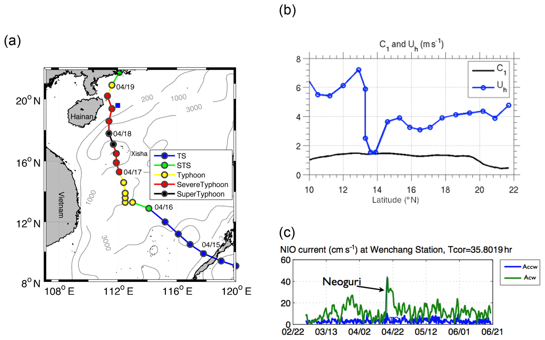
Figure 1(a) Track of Typhoon Neoguri (2008) from JTWC; blue square represents Wenchang where there were ADCP observations; (b) translation speed (Uh; unit: m s−1) and the first baroclinic wave speed (C1; unit: m s−1) along the TC track; (c) clockwise (Acw) and counter-clockwise (Accw) rotary current amplitude (m s−1) from current measurement at Wenchang. TS: tropical storm; STS: strong tropical storm.
2.2 Ocean model
We use the China Sea Multi-scale Ocean Modeling System (CMOMS) (Gan et al., 2016a, b) in this study. CMOMS is based on the Regional Ocean Modeling System (ROMS) (Shchepetkin and McWilliams, 2005), and the model domain covers the northwest Pacific Ocean (NPO) and the entire China Seas (Bohai, Yellow Sea, East China Sea, and SCS) from approximately 0.95∘ N, 99∘ E in the southwest corner to the northeast corner of the Sea of Japan. The horizontal size of this grid array decreases gradually from ∼10 km in the southern part to ∼7 km in the northern part of the domain. Vertically, we adopted a 30-level stretched generalized terrain-following coordinates.
The model was forced with 6-hourly actual wind speeds of typhoon Neoguri obtained from the Cross-Calibrated Multi-Platform (CCMP) dataset, with a horizontal resolution of 0.25∘ (Atlas et al., 2011; http://data.remss.com/ccmp/v02.0/Y2008/, last access: 16 September 2020). Wind stress is calculated based on the bulk formulation by Fairall et al. (2003). The daily mean air temperature, atmospheric pressure, rainfall or evaporation, radiation, and other meteorological variables from 15 to 18 April 2008 from the NCEP/NCAR Reanalysis 1 were used to derive the atmospheric heat and fresh water fluxes. External forcing of depth-integrated velocities (U,V), depth-dependent velocities (u,v), temperature, T, and salinity, S, at the lateral boundaries were obtained from the Ocean General Circulation Model for the Earth Simulator (OFES) (Sasaki et al., 2008). Open boundary conditions from Gan and Allen (2005) were applied at the open boundaries.
The model was spun up from 1 January 2005 with winter initial fields (temperature and salinity) obtained from the last 3-year mean fields of a 25-year run that is initialized with the World Ocean Atlas (2005) (WOA05; Locarnini et al., 2006; Antonov et al., 2006) data and forced by wind stress derived from climatological (averaged from 1988 to 2013) monthly Reanalysis of 10 m Blended Sea Winds released by the National Oceanic and Atmospheric Administration (https://www.ncei.noaa.gov/thredds/catalog/uv/monthly/catalog.html, last access: 16 September 2020). The dynamic configuration and numerical implementation of the CMOMS system are described in detail in Gan et al. (2016a, b).
We have thoroughly validated the CMOMS by comparing simulated results with those obtained from various measurements and findings in previous studies. In particular, we have validated the extrinsic forcing of a time-dependent, three-dimensional current system in the tropical NPO, transports through the straits around the periphery of the SCS, and corresponding intrinsic responses of circulation, hydrography, and water masses in the SCS (Gan et al., 2016a). We have also validated the circulation of CMOMS by providing consistent physics between the intrinsic responses of the circulation and extrinsic forcing of flow exchange with adjacent oceans (Gan et al., 2016b). The model is also validated with available Argo (https://data-argo.ifremer.fr/geo/pacific_ocean/, last access: 16 September 2020) temperature profiles (not shown), observed sea surface temperature (SST), and currents from a time series current meter mooring during Neoguri, as described below.
Three-dimensional, hourly-mean dynamic, and thermodynamic variables from 10 April to 10 May 2008 were used to examine the near-inertial oscillations in this study. Because the inertial period (IP) in the SCS is larger than 32 h (near 22∘ N), the error induced by the hourly model output is <3 %.
3.1 Characteristic response to the TC
The evolution of the response to the TC in the ocean with the existence of a coastal jet in the SCS is presented according to different stages of the TC forcing. During the pre-storm stage (PS), before Neoguri entered the SCS on 14 April, the wind stress was relatively weak (<0.1 Pa). A prominent jet current separated from the Vietnamese coast flowing northeastward near 16∘ N (Fig. 2a) and characterized the circulation in the western part of the SCS. The jet resulted from the (summer) monsoon-driven strong coastal current over narrow shelf topography off Vietnam and it persisted as a distinct circulation feature in the SCS during summer. The northward-flowing coastal current separated from the coast and overshot northeastward into the SCS basin as it encountered the coastal promontory in central Vietnam (Gan and Qu, 2008).
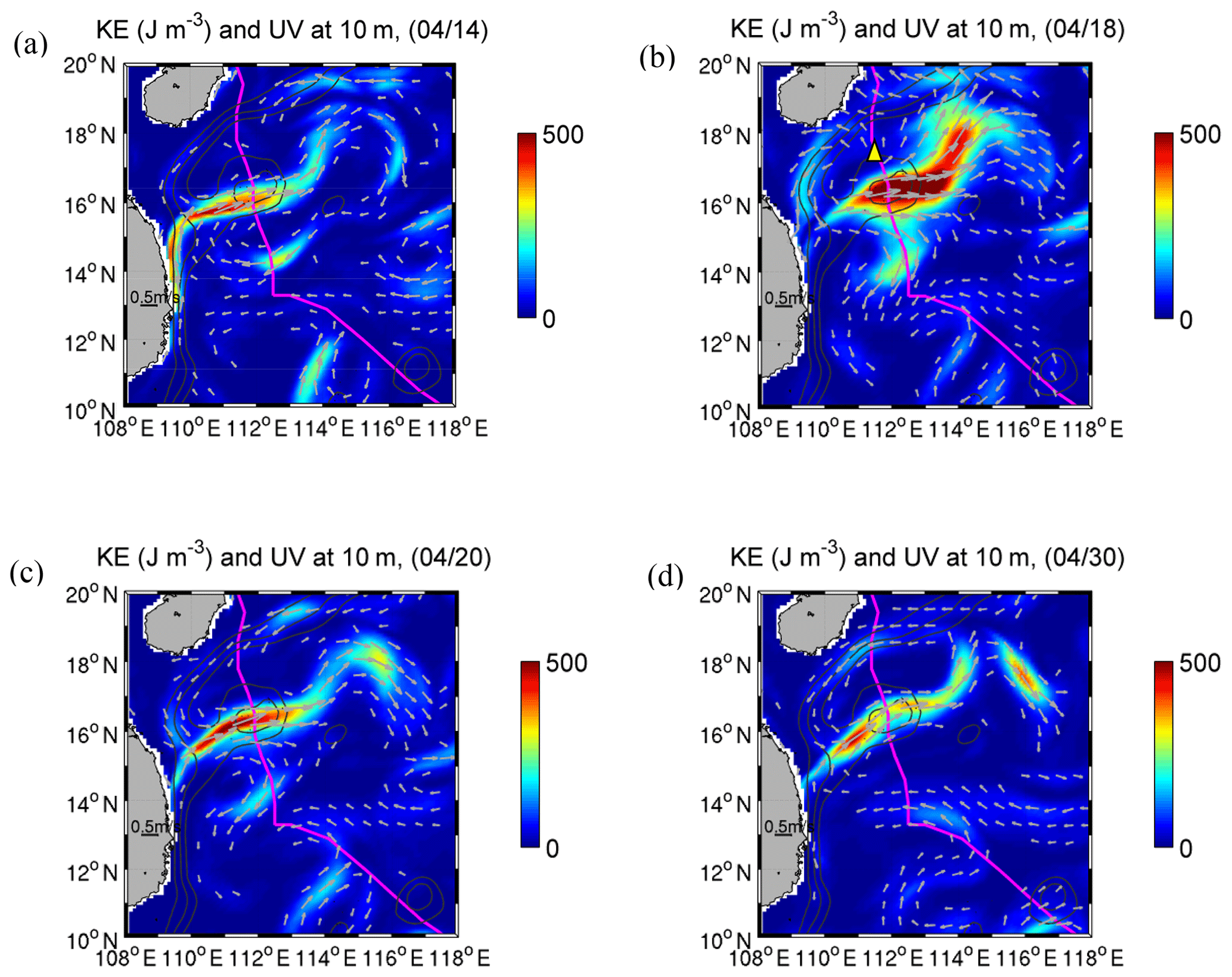
Figure 2Daily mean KE (J m−3, colour contour) and current vectors (arrows) at 10 m (a) on 14 April of the pre-storm stage (PS), (b) on 18 April during the strongest wind forcing of the forced stage (FS), (c) on 20 April after the end of the FS, and (d) on 30 April during the relaxation stage (RS). The grey contours are the 200, 500, and 1000 m isobaths. The magenta line represents TC track. Yellow triangle on 18 April represents the TC location. The TC was located beyond the plotting domain during the other 3 d, as shown in Fig. 1a. The velocity magnitudes <0.2 m s−1 are not shown in the vectors.
The jet formed negative (positive) geostrophic vorticity (ζg) to the south (north), with the minimum (maximum) Rossby number (ζg f−1) <−0.2 (>0.2) near 15.8∘ N (16.8∘ N). During the forced stage (FS; Fig. 2b) between 15 and 19 April, the SCS was under the direct influence of Neoguri, the wind forcing became significantly stronger (>0.1 Pa), the kinetic energy (KE) near the surface (10 m) intensified significantly (>500 J m−3) to the east of the TC, and the coastal jet was suppressed by southward flow. Meanwhile, a strong local divergence and upwelling formed at the surface and generated a strong cooling (∼1.5 ∘C) belt along the TC path that lasted for more than a week. The cooling zone radiated hundreds of kilometres away from the core of the TC. These features were well captured by the TC-induced temperature difference between 19 and 14 April from both simulated (Fig. 3a) and observed SST (Fig. 3b) (https://podaac-opendap.jpl.nasa.gov/opendap/allData/ghrsst/data/GDS2/L4/GLOB/JPL/MUR/v4.1/, last access: 16 September 2020). After the end of the FS on 20 April (Fig. 2c), the jet returned to its pre-storm intensity and shifted slightly northward (Fig. 2c) when the TC centre approached the coast (Fig. 1a). Afterwards, during the relaxation stage (RS) after 20 April (Fig. 2d), the wind forcing from the TC decreased to <0.05 Pa.
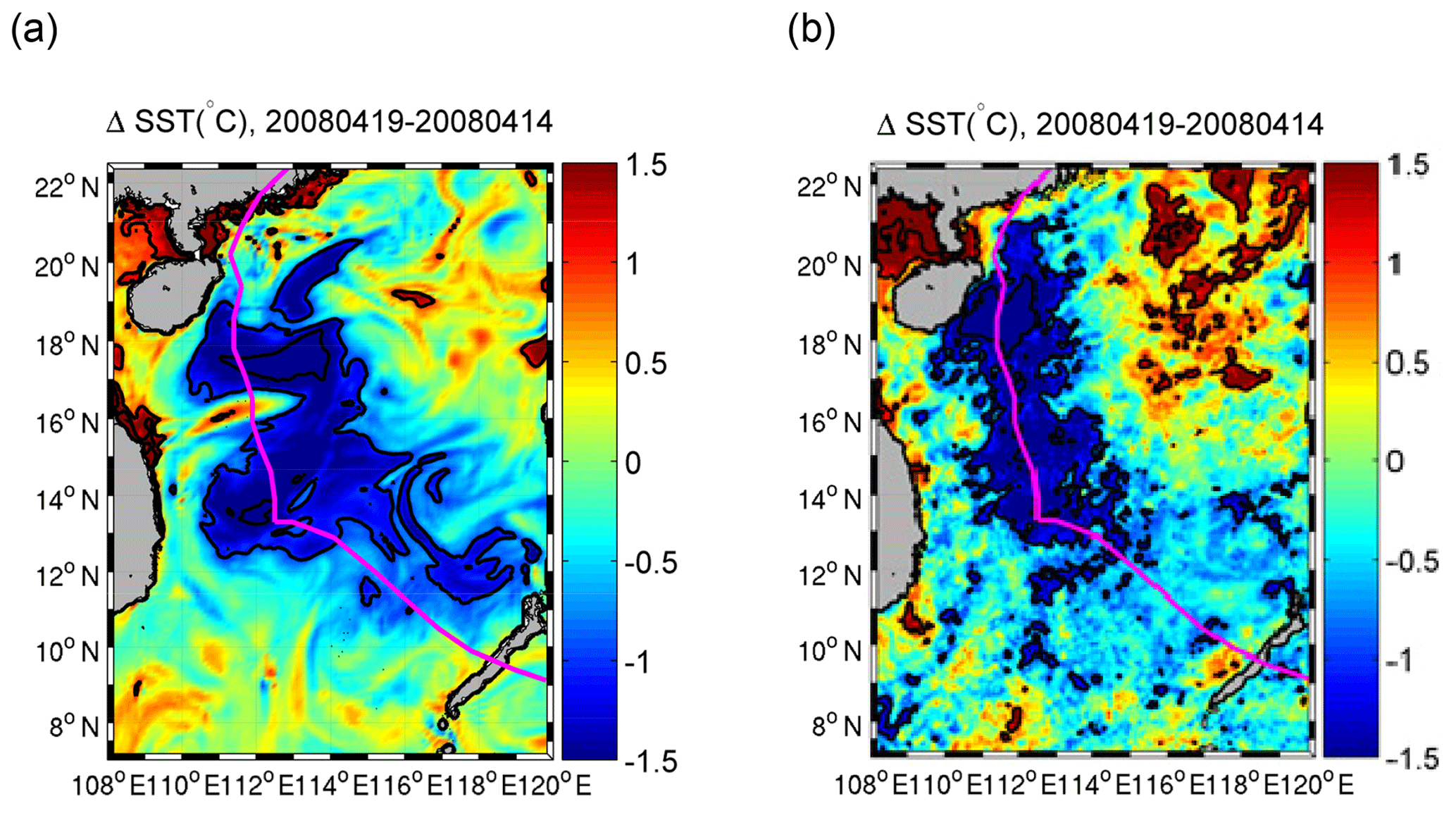
Figure 3ΔSST (19 April–14 April) from (a) model results and (b) GHRSST JPL MUR satellite products. The pink curve indicates to the trajectory of the TC Neoguri.
The rotary spectrum shows that the near-inertial response of surface currents to the TC occurred near the local inertial frequency (f=0.028 cph, cycles per hour) at Wenchang station (19.6∘ N, 112∘ E) during the model simulation period (10 April–5 May) (Fig. 4). The clockwise rotary spectra are calculated by
where Puu, Pvv, and Quv are auto and quadrature spectra, respectively (Gonella, 1972). This simulated result is highly consistent with the observations in the lower-frequency band. We found that the correlation coefficients of near-inertial band-passed velocity between acoustic Doppler current profiler (ADCP) and model simulation at Wenchang station were 0.62 and 0.57 for the east–west (u) and north–south (v) component, respectively, which indicated that the model captured reasonably well the NIOs under the influence of the background circulation of the SCS. There inevitably existed model–observation discrepancies, such as differences in velocity magnitude (∼0.06 m s−1) at near-inertial band and rotary spectra at the higher frequency (Fig. 4). The discrepancies could have been caused by many factors, such as the lack of mesoscale and sub-mesoscale processes in the atmospheric forcing field, the linear interpolation process of the atmospheric forcing (Jing et al., 2015), and not resolving the oceanic subscale processes by the current model resolution. However, these discrepancies will not undermine the discussion about the process and mechanism of near-inertial energy response to the TC and jet in this study.
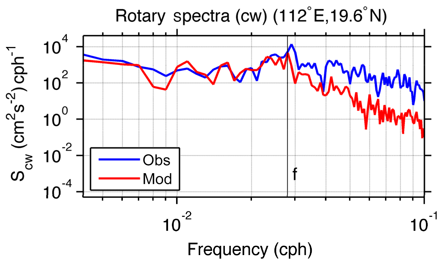
Figure 4Rotary spectra of clockwise component (upper 10 m) at Wenchang (19.6∘ N, 112∘ E) from model simulations (red) and observations (blue).
3.2 Near-inertial response in the upper ocean
We adopted the complex demodulation method successfully used in previous NIO studies (Gonella, 1972; Brink, 1989; Qi et al., 1995) to extract the inertial current signal. The simulated horizontal currents (uh) were analysed for inertial currents (ui). The inertial currents contain clockwise (cw) and counter-clockwise (ccw) rotating components:
where ui and vi are the eastward and northward inertial currents at 10 m in the mixed layer (ML) and A and ϕ are the amplitude and phase of the rotary currents, respectively. Subscripts represent the clockwise (cw) and counter-clockwise (ccw) rotating direction, and f is the local Coriolis coefficient. To obtain the amplitude and phase, we performed harmonic analysis daily with each segment over one inertial period (IP). Then the rotary amplitude and phase were calculated following previous studies (Mooers, 1973; Qi et al., 1995; Jordi and Wang, 2008).
The time evolution of the daily rotary currents during the FS and RS in the surface layer varied spatially and was related to the intensity and translation speed of the TC. On 15 April during PS, Neoguri mainly affected the region south of 13∘ N, with a relatively fast translation speed (Uh>3C1, Fig. 1b) and weaker intensity (Vmax∼35 m s−1). In most areas, cw rotary currents were strong (Acw>0.1 m s−1), yet decayed quickly after 3 d (less than two IPs; Fig. 5a), while the magnitudes of ccw currents were very small (Fig. 5b). After 18 April, Neoguri moved into the region between 14 and 18∘ N, where it intensified more than 40 % but moved slower with Uh∼2C1. Both the cw and ccw currents possessed larger intensities than in the southern region. The induced cw currents displayed an obvious rightward bias, where the enhanced inertial currents extended to ∼350 km to the right of the track and to ∼<150 km to the left of the track. This extension of horizontal scale was related to the region with a wind stress Pa in Neoguri.
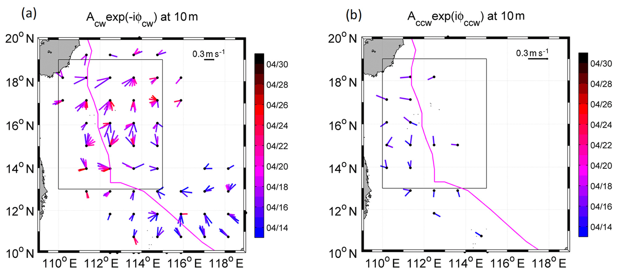
Figure 5Time series, represented by colour bar, of daily (a) clockwise and (b) counter-clockwise rotary current vectors from 14 to 30 April during different stages of the TC forcing, signifying the response of the current to the local wind rotation. For the clockwise (counter-clockwise) component, only currents with a magnitude larger than 0.2 (0.05) m s−1 are shown. The black box represents the forced region.
The maxima of the ccw component were located to the left of the TC's path where the wind vector (Fig. 6) rotated in the same direction as the ocean currents presented in Fig. 5. The connection between the right (left) bias of the cw (ccw) currents with the rotation direction of the wind vector is in agreement with the explanation of Price (1981). Two to three IPs (>6 d) after the direct forcing, the cw currents remained significant (>0.2 m s−1) in an area extending from 110 to 116∘ E. In contrast, the ccw components dissipated quickly, within ∼1 d after the wind forcing stopped. This short duration of the forced inertial motion is in agreement with previous studies (Jordi and Wang, 2008).
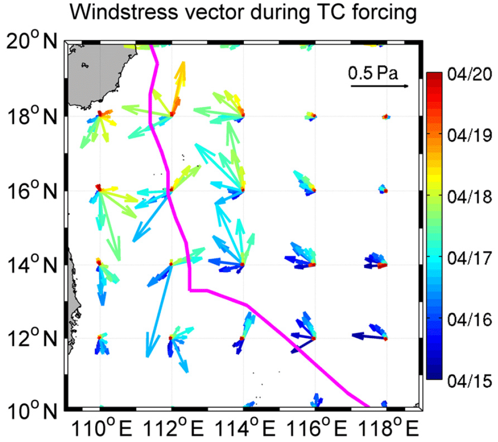
Figure 6Time series of 6-hourly wind stress vectors during the forced-stage (FS) from 15 to 20 April.
Besides the intensity and duration, we also looked at the frequency shift () and the horizontal scale of the NIOs. The frequency shift from the local inertial frequency was estimated from the temporal evolution of the phase of the rotary current: . In the FS, the maximum frequency shift occurred near the jet (15 to 16∘ N, 112 to 115∘ E), where δω≈0.08f (, Δ t=3 d, s−1 at 16∘ N). The horizontal scale was estimated from the spatial variation in the rotary current by calculating the horizontal wave number in the meridional direction as . The largest wave number rad m−1 was also found near the jet.
3.3 Characteristic near-inertial energy
3.3.1 Response in the upper layer
We focused on the area between 110–115∘ E and 13–19∘ N (box in Fig. 5a), defined as the forced region, where the strongest NIO was produced during the FS of Neoguri. We calculated the wind-induced near-inertial energy flux (or the wind work) using τi⋅ui, where τi is the band-passed near-inertial wind stress and ui is the near-inertial current at the surface (Silverthorne and Toole, 2009). A fourth-order elliptic band-pass filter (Morozov and Velarde, 2008) was applied to obtain near-inertial motion with a band ranging from 0.8 f to 1.2 f, where f is the local Coriolis coefficient. The time series of domain-averaged τi⋅ui over the forced region reveals that significant energy input took place during the FS, with the peak value about W m−2 on 17 April (Fig. 7). Under this large wind energy input, the area-averaged depth-integrated KEni (or AKEni hereafter) in the upper layer (0–30 m) increased significantly from its pre-storm value to a maximum ∼1500 J m−2 during the FS, with an increase rate of about W m−2 (Fig. 7a). We set 0–30 m as an upper layer based on domain mean stratification and current (vorticity) vertical structure. Despite the continuous positive wind energy flux, the AKEni in the upper layer plateaued, indicating that a large amount of the wind energy was either propagating out of the forced region or was lost to the lower layers due to entrainment. The detailed mechanisms are discussed in the following sections. After the peak of FS, the wind work decreased significantly with a small negative value around the end of the FS. The AKEni decreased to one half of its peak value within 2 d (decrease rate was about W m−2). After that, the wind work was almost negligible, and the decrease rate of AKEni became smaller ( W m−2).
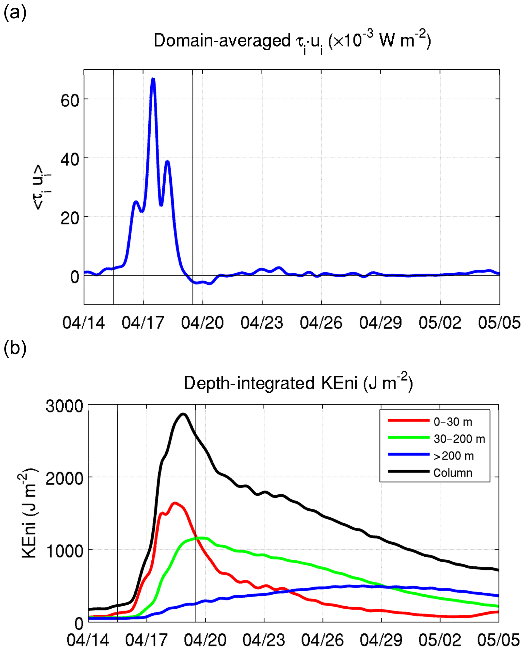
Figure 7Time series of (a) the area-averaged wind energy flux into the near-inertial band (unit: 10−3 W m−2) and (b) depth-integrated KEni (J m−2) in the forced region for different layers.
3.3.2 Response at depths
During the FS, the AKEni in the upper 200 m constituted ∼90 % of the total AKEni in the whole water column, while the AKEni between 30 and 200 m alone accounted for ∼30–50 % (Fig. 7b). The AKEni in this mid-layer had a temporal evolution different from that in the near-surface layer. It reached its maximum on 20 April, around 1.5 d later, and was more than 70 % of the peak value of the AKEni in the upper layer (∼1700 J m−2). Compared to the upper-layer AKEni, the mid-layer AKEni during FS increased slightly more slowly ( W m−2), while from 20 April to 5 May during RS it decreased much more slowly ( W m−2), and the AKEni became greater than that in the upper layer at the end of FS. The AKEni below 200 m was much smaller but increased continuously from 17 to 29 April, with a rate of about W m−2, which was comparable to the AKEni rate of decrease in the 30–200 m layer. The AKEni in this deep layer became greater than that in the upper layer after 25 April and that in the layer 30–200 m after 29 April; the deep layer reached its maximum value ∼10 d after the ending of the FS.
Spatially, two relatively large KEni patches below the upper layer were located to the north and south of ∼16∘ N (Fig. 8a). Their horizontal scales, influenced by near-inertial waves, were much smaller compared with those in the upper layer. The region with relatively large KEni in the layer between 30 and 200 m was located near the jet currents, with stronger value during FS than during RS (Fig. 8a, b). These results suggest that the KEni in this layer might have been determined by both vertical propagation of the near-inertial gravity wave and horizontal advection of KEni of the background current. Similar horizontal distribution also occurred below 200 m (Fig. 8c, d). In contrast to the layer above, the relatively large value during RS on 30 April indicated a downward propagation of KEni into the deeper layer. Around the saddle zone west of the Xisha Islands, a relatively large KEni below 200 m aligned with the 1000 m isobath and might reflect a topographic effect on the near-inertial wave.
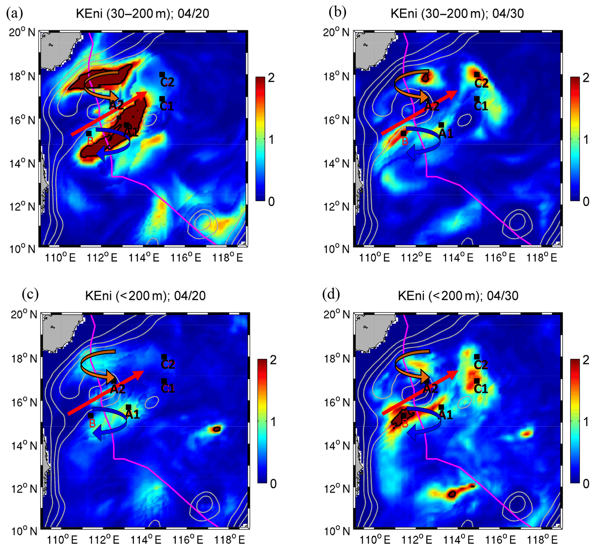
Figure 8Daily averaged KEni (KJ m−2) of layers (a, b) 30–200 m and (c, d) <200 m on (a, c) 20 April during FS and (b, d) 30 April during RS. The thick red arrows show the location of the jet (Fig. 2), while the blue curved arrows indicate regions with relative vorticity ζ<0 and the orange curved arrows indicate regions with ζ>0. Stations A1 and A2 are on the right side of the TC track at the northern (A2) and southern (A1) sides of the jet, respectively. Stations C1 and C2 are corresponding stations in the far field. Station B is located in the upstream area of the jet.
3.4 Vertical propagation of near-inertial energy
It is clear that the distribution of the KEni was mainly controlled by the propagation of near-inertial wave energy both horizontally and vertically as well as by the background jet. In order to understand the KEni distribution in the deeper water inside the forced region and in the far field, we selected four different locations, marked as A1, A2, C1, and C2 in Fig. 8a–d, for the analysis of the KEni evolution during the FS and RS. Among them, A1 (15.7∘ N, 113∘ E) and A2 (16.9∘ N, 112.5∘ E) are on the right side of the TC track, inside the forced region and situated about 200 km apart from each other at the northern (A2) and southern (A1) sides of the jet, respectively. C1 (16.9∘ N, 114.9∘ E) and C2 (18∘ N, 114.9∘ E) are the corresponding stations in the far field where relatively strong KEni intensification occurred.
3.4.1 Forced region (stations A1 and A2)
South of the jet at station A1
The time series of the band-passed inertial velocity ui as a function of depth shows that there was an upward phase propagation, in which ui, in the layers below 100 m was leading the upper 50 m (Fig. 9a). Accompanying this phase propagation was a downward propagation of surface KEni, which was represented by the lowering of the ui maxima as a typical Poincaré wave (Kundu and Cohen, 2008). There were two phases of vertical energy propagation: (1) during FS, there was a rapid extension of the large ui maxima to below 100 m from 17 to 20 April, and (2) during RS, the centre of the large ui value descended from ∼100 to 280 m from 25 April to 5 May. The vertical propagation velocity, Cgz, estimated from this downward transport, was ∼17 m d−1.
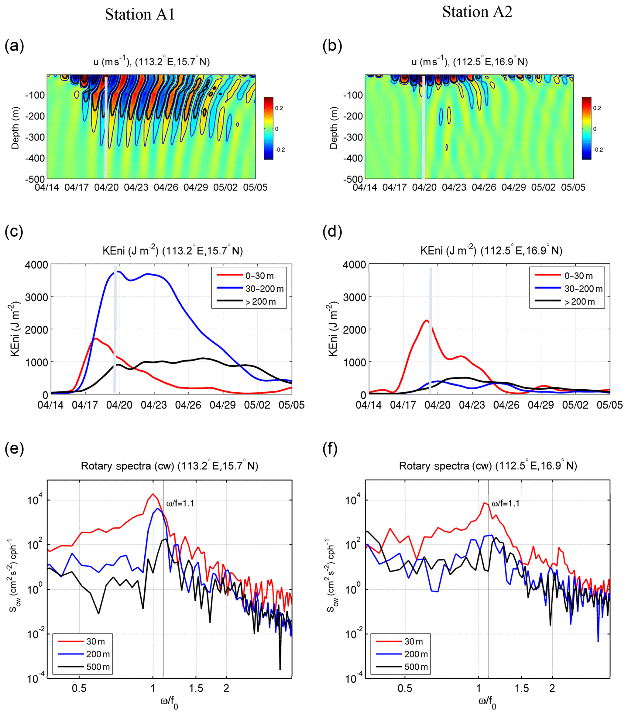
Figure 9Time series of (a, b) ui (m s−1), (c, d) KEni (J m−2), and (e, f) rotary spectra (cw component) at locations A1 (a, c, e) and A2 (b, d, f).
During the first phase, the KEni in the top 30 m and in the 30–200 m layer shared a similar rate of increase on 17 April, indicating that the enhancement of KEni at 30–200 m was related to the entrainment between the upper and deep layer (Fig. 9c). While the KEni in the upper 30 m decreased quickly from 18 April, it kept increasing at depths from 30 to 200 m, suggesting that other contributing mechanisms existed besides the entrainment. The KEni below 200 m also experienced notable intensification, with a smaller rate of increase than that found in the 30–200 m layer (Fig. 9c). Because the viscous effect is small in the deeper water, this enhancement of the KEni was most likely associated with the propagation of an inertial-gravity wave.
During the second phase, the KEni in the 30–200 m layer decreased significantly at station A1, indicating the existence of either downward or horizontal energy transport. From the linearized inertial-gravity wave equation under the influence of background vorticity, Cgz can be obtained by Morozov and Velarde (2008):
where ω≈1.08f is the frequency with maximum Scw at 200 m (Fig. 9e); is the effective Coriolis coefficient; and at A1. m is the vertical wave number that we chose to be the first baroclinic mode under a two-layer approximation based on the stratification (blue line in Fig. 10a). From Eq. (2), Cgz was about 19.1 m d−1, which was in the same range as the modelled Cgz. Consistent with the case of ( in Kunze (1985), the background vorticity in our case accounted for more than 90 % of the modification of the magnitude of the wave dispersion property. Meanwhile, the KEni in the layer below 200 m did not increase notably, suggesting that other mechanisms besides vertical propagation of the near-inertial gravity wave might have been important in the evolution of KEni in water deeper than 200 m.
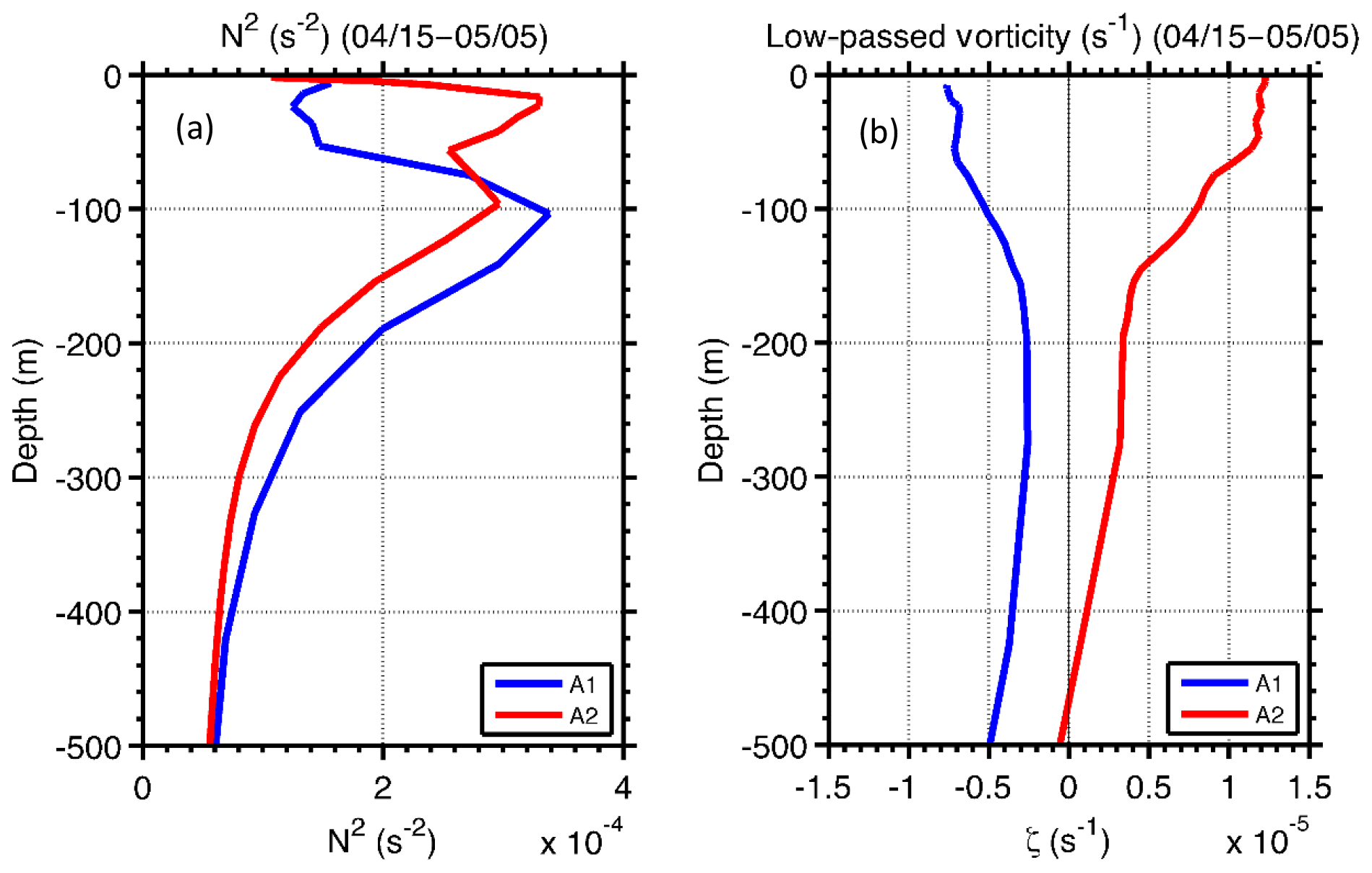
Figure 10Time-averaged (a) N2 (s−2) and (b) low-passed (3 d) vorticity from 15 April to 5 May at locations A1 (red) and A2 (blue).
North of the jet at station A2
At location A2, strong ui was mainly trapped in the water above 100 m, and below 100 m ui<10 cm s−1. It returned to its pre-storm magnitude after five IPs (Fig. 9b). This constraining of vertical propagation is likely associated with the vertical scale of the strong positive background vorticity (Fig. 10b). The KEni was generally smaller than that at A1, and relatively large energy was found only in the ML (Fig. 9d). Cgz at A2, estimated from Eq. (2), was 2.1 m d−1 ( s−1, and m), which was about 1/10th of that at A1. This is consistent with the lack of a distinct pattern of vertical propagation of NIOs at this station, as shown in the band-passed ui (Fig. 9b), and the presence (absence) of a near-inertial peak of Scw at 10 m (200 m) (Fig. 9f).
3.4.2 Far-field region (stations C1 and C2)
C1 and C2 are located ∼400 km to the right of the forced region. During the FS, ui (Fig. 11a, b) and KEni (Fig. 11c, d) in the upper layer were smaller than those at those stations in the forced region due to the weaker TC influence. Only a small downward propagation was discerned during the FS (Fig. 11a, b). However, notable intensification of the KEni occurred in the layers below the upper layer after 23 April. At C1, the Scw at 10 m had a small red shift, while the Scw at 200 and 500 m displayed blue shifts with peaks near 1.07f (Fig. 11e). The difference between Scw in the upper layer and in the layers below implies another source of KEni other than local inertial-gravity wave vertical propagation.
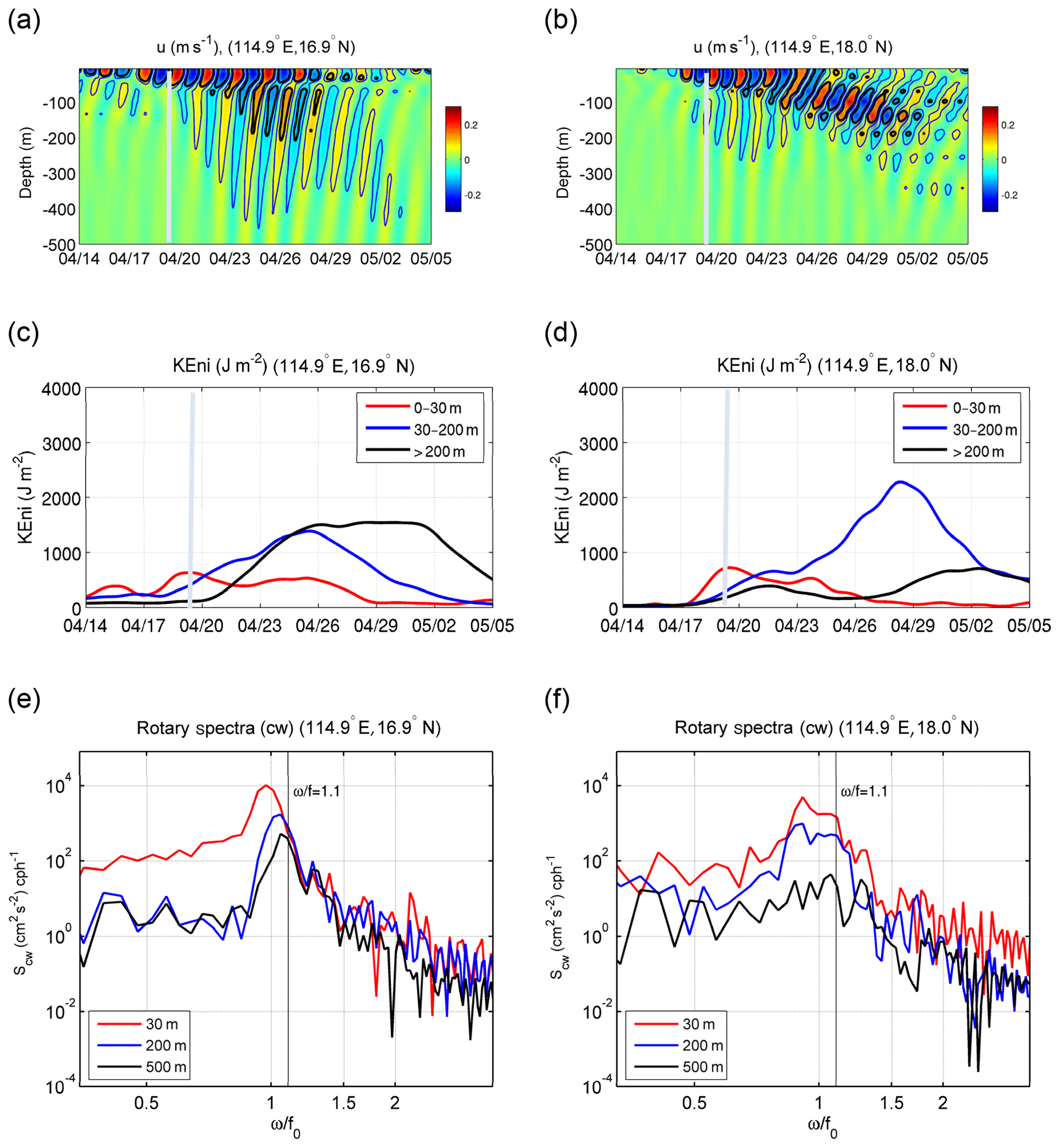
At C2, downward energy propagation appeared after 23 April, reaching 100 m from the surface within 7 d, giving Cgz=14.3 m d−1 (Fig. 11b). Unlike C1, the intensification was mainly in the 30–200 m layer. The Scw at both 10 m and 200 m had a broad energy band near the local f (Fig. 11f). Because and feff=1.06f, Cgz estimated from Eq. (2) had an upward propagation ( m d−1), which cannot explain the downward propagation here. The linearized wave theory, with the consideration of Doppler drift due to background currents, does not seem to be valid in this location. We will discuss this issue in the next section.
We utilized the KEni equation to provide a further analysis of the source of KEni in the water column. Because the horizontal component of near-inertial kinetic energy is significantly larger than the vertical component (Hebert and Moum, 1994), we used the horizontal component to represent the KEni. The KEni budget can be obtained from the horizontal momentum equation:
where KEni is the near-inertial energy; ui and uh are the near-inertial velocity vector and horizontal velocity, respectively; p is pressure; ρ0 is the reference density; ∇h is the horizontal gradient operator; w is the vertical velocity; υ is the viscosity coefficient; and the angle bracket represents band-passed filtering on the near-inertial band. The PRES term on the right side of equation represents the pressure work on the KEni, which is associated with the inertial-gravity wave propagation. NLh and NLv represent the horizontal and vertical divergence of energy flux that include the effects of (1) the advection of KEni due to background currents and (2) the straining of the wave field due to the background shear currents. Zhai et al. (2004) found that the geostrophic advection of KEni contributed most of the NLh and was the main mechanism for transporting the NIOs in the absence of baroclinic dispersion of inertial-gravity waves. It was also found to be more important than the dispersive processes along the Gulf Stream or shelf-break jet. VVISC is the vertical viscous effect. As before, we integrate this equation vertically in three layers: the upper layer (0–30 m), the subsurface layer (30–200 m), and the deep layer (>200 m). In the following sections, the AKEni budget is considered in entire forced region (Fig. 5) as well as at the specific stations along the jet.
4.1 Mean balance
Figure 12 shows the time series of the AKEni budget over the entire forced region defined in Fig. 5. The time-averaged horizontal distributions of each term are presented in Fig. 13. During the FS, the increase in AKEni in the upper layer was mainly attributed to the wind energy input because the VVISC term was 1 order larger than the other terms, with a maximum of W m−2 on 17 April (Fig. 12a). The time-integrated VVISC during the FS was 2.15×10³ J m−2 (Table 1). Stronger VVISC in the upper 30 m occurred in the region between 14∘ N and 18∘ N (Fig. 13a) along the TC track with a rightward bias, similar to the distribution of current intensity (Fig. 5c). Like the wind work during the FS (Fig. 7a), VVISC became negative after 19 April, indicating the AKEni removal by negative wind work. The influence of VVISC extended to the 30–200 m layer and provided a positive energy flux ( J m−2) in this layer (Figs. 12b, 13b). The effect of VVISC in the deep layer was negligible (Fig. 12c).
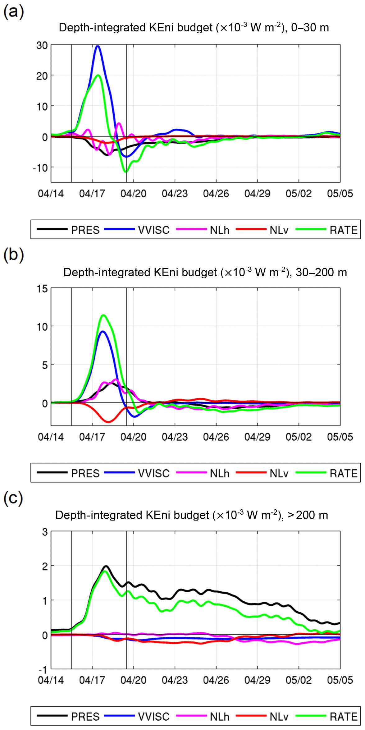
Figure 12Time series of area-averaged, depth-integrated KEni budget for (a) 0–30 m, (b) 30–200 m, and (c) >200 m in the forced region. Terms represent (unit: W m−2) pressure work (PRES), vertical viscous effect (VVISC), horizontal non-linear interaction (NLh), vertical non-linear interaction (NLv), and changing rate of KEni (RATE). The vertical lines separate the pre-storm stage, FS, and RS during the TC forcing.
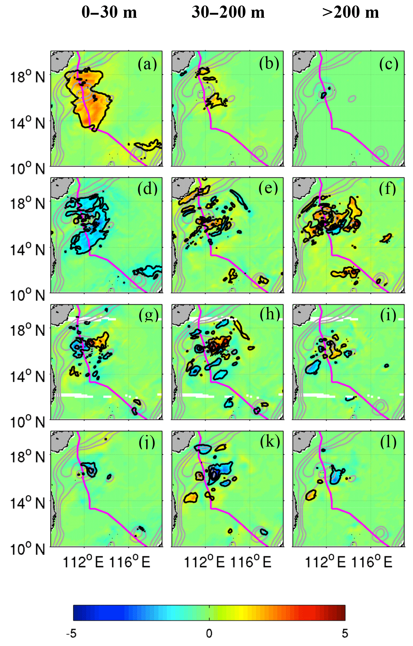
Figure 13Horizontal distribution of time-averaged (15 April–5 May) depth-integrated KEni budget in different layers: 0–30 m (left column), 30–200 m (middle), and >200 m (right). The terms represented are (unit: W m−2) (a–c) VVISC, (d–f) PRES, (g–i) NLh, and (j–l) NLv.
Table 1Time integrated KEni budget (unit: ×103 J m−2) during the FS and RS.
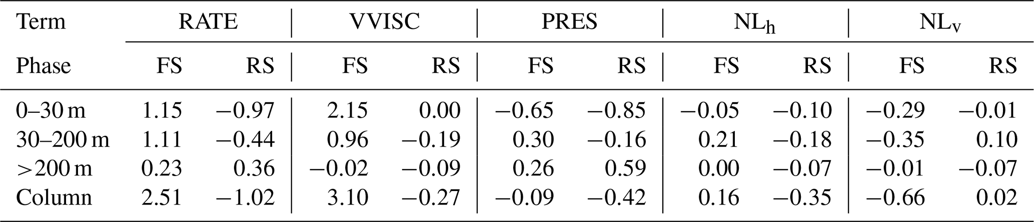
Shortly (∼1 d) after the large injection of KEni into the upper layer during the FS, the PRES became significant (Fig. 12a, Table 1), and its horizontal distribution resembled that of VVISC (Fig. 13a, d), suggesting that PRES radiated the KEni out of the forced region. It provided a negative KEni flux in the upper layer ( J m−2), which was largely compensated for by the positive flux in deeper layers (Table 1). This suggests that, during the FS, the main role of the pressure work was to transport the KEni from the upper layer to the deep layers, and <15 % of the KEni was horizontally propagated outside the forced region.
During the RS, the VVISC was relatively small in the upper layer and it accounted for one-third of the AKEni removal in the layers below (Table 1). The PRES became a major sink for AKEni in the ML ( J m−2) and subsurface layer ( J m−2) but was the major source in the water below 200 m. The AKEni loss due to the horizontal wave propagation outside the forced region was J m−2, accounting for about 40 % of the total loss in the whole water column.
Nonlinear advection terms had an important influence in the top 200 m but made little contribution to the AKEni budget in the water below 200 m (Fig. 12, Table 1). The horizontal effects of NLh and NLv in these layers were mainly limited to a smaller region, as compared to the VVISC and the PRES; and their relatively large values occurred near the slope and the jet (Fig. 13).
In the upper layer, NLh advected the KEni from the source region; NLh had positive and negative values on the eastern and western sides of the TC track, respectively (Fig. 13g). Similar features, but with much weaker amplitude, were found in the layers below (Fig. 13h, i). During the FS, in the 30–200 m layer, the domain-averaged NLh was positive (0.21×10³ J m−2), indicating a possible extraction of the KEni from background flows. NLv was a strong energy sink in the upper 200 m ( J m−2). The TC wind field generated a strong surface horizontal divergence and upwelling around 16–17∘ N (Fig. 4b). As a result, the smaller KEni in the lower layer was advected to the surface east of the Xisha Islands. This lower KEni generated a negative gradient with ambient water and resulted in the strong eastwards transport of KEni in the eastward jet current. As a result, a positive NLh centre was located around the area with the strongest negative NLv, and a negative NLh centre lay to the west of the positive maximum of NLh. During the RS, NLh became negative for all layers and provided of the total KEni loss in the water column ( J m−2), while NLv over the whole water column was significantly reduced.
4.2 Role of the jet
We further show the distinct AKEni balance in the southern and northern sides of the jet. During the FS, VVISC at A1 on the southern side of the jet was the dominant AKEni source in both the upper layer and the 30–200 m layer (Fig. 14a, b), consistent with the large vertical scale on the southern side of the jet due to local negative vorticity. The enhancement of near-inertial currents in the upper layer and the concurrent current divergence resulted in the vertical oscillation of isopycnals (pressure) below the upper layer at this station. During this pumping process, the AKEni in the upper layer was partly transported downward by the PRES and partly by the NLv. During the RS, the PRES became the main factor in the AKEni budget. It changed from source to sink in the 30–200 m layer because of less downward KEni flux from the upper layer. In the deeper layer, the negative PRES indicated that there was a near-inertial wave propagating away from this location. The positive AKEni flux provided by NLh weakened the effect of the negative PRES.
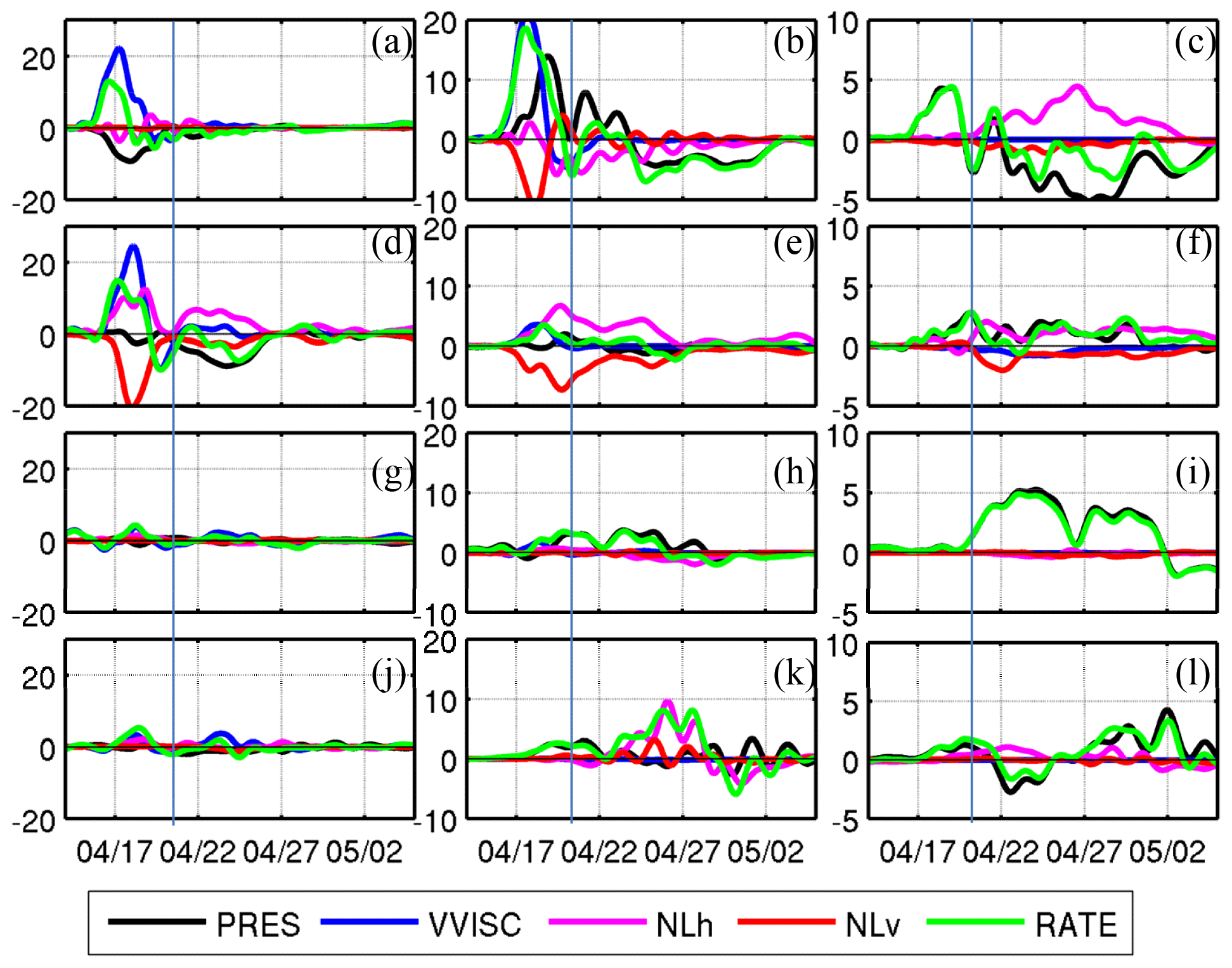
Figure 14Time series of KEni budget at locations: A1 (a–c), A2 (d–f), C1 (g–i), and C2 (j–l) in the following layers: 0–30 m (left column), 30–200 m (middle column), and >200 m (right column). Presented are (unit: W m−2) (a–c) VVISC, (d–f) PRES, (g–i) NLh, and (j–l) NLv.
During the FS at A2 on the northern side of the jet, VVISC in the upper layer (Fig. 14d) had slightly larger magnitude than that at A1. However, it greatly decreased to W m−2 below the ML (Fig. 14e), which suggested that the smaller vertical scale on the northern side of the jet limited the deep penetration of the wind energy in this location. Compared to A1, the NLv was much stronger in the upper layer, and about one half of the lost energy was compensated for by the NLh. The PRES was negligible compared to that at A1 (Fig. 14d–f). During the RS, the PRES in the ML became a notable sink after 21 April and was accompanied by a positive NLh (Fig. 14d). This suggests that the strong jet increased the AKEni through either advection or wave propagation due to PRES as a result of jet-NIO interaction at this station. In the deeper layer, the PRES provided a positive AKEni flux. From the spectral analysis, the wave at 500 m had a large blue shift of >0.15f (Fig. 9f) that cannot be explained by the background vorticity alone. The wave likely originated from the northern latitude.
In the far field at stations C1 and C2, where there was no direct wind forcing from the TC, surface forcing (VVISC) was relatively small during the FS (Fig. 14g, j). Therefore, horizontal transport of energy is needed to sustain the KEni intensification at these two locations (Fig. 11c, d). At C1, which was on the southern side of the jet (Fig. 8) and had a negative background vorticity, the PRES was the main source of AKEni in both subsurface and deep layers (Fig. 14h, i). The existences of the blue shift near the local inertial frequency (Fig. 11e) and of the negative background vorticity suggests the presence of a southward-propagating near-inertial wave towards C1 from northern region. Because C2 lies near the northeastward turning point of the jet (Fig. 8), the nonlinear effect became significant in the 30–200 m layer where the jet was strongest (Fig. 14k). After the enhancement of AKEni in the subsurface layer, the PRES further transported the KEni downwards and became the major source for the increase in AKEni in the deep layer after 27 April (Fig. 14l). The northeast current advected the lower-frequency NIO from the lower latitude towards the higher latitude, C2, which explains the red shift of the NIO at this location (Fig. 11f).
TCs force the ocean to form NIOs. The response of NIOs is largely associated with the different forcing stages of the TCs and background flow. Due to spatiotemporally limited measurements, our understanding of the process and mechanism that govern the NIO response is mainly based on theories that are constrained by idealized assumptions. In this study, we utilize a well-validated circulation model to investigate the characteristic response of KEni to a moderately strong TC (Neoguri) with observed strong KEni and to a unique background circulation.
The near-inertial currents in the upper layer strengthened significantly during the TC forced stage and displayed a clear rightward bias due to stronger wind forcing and the resonance between the wind and the near-inertial currents. The distribution of near-inertial currents and the associated rotary spectra showed that the propagation patterns of NIOs varied greatly from location to location and were closely linked to the influences of the background jet.
We calculated the KEni balance to diagnose spatiotemporally varying responses and processes of the near-inertial signals in terms of different forcing stages of the TC. Results show that during the forcing period, the vertical viscous term, which represents the wind work and entrainment at the base of the upper layer, was the KEni source in the upper layer. Around 0.5 IP after the maximum TC forcing, the pressure work became the main KEni sink in the upper layer, transporting KEni in the ML into the deeper layers through inertial pumping. In the meantime upwelling, caused by the TC-enhanced divergence, advected smaller KEni from deeper layers to weaken the KEni in the upper layer.
During the TC relaxation stage, the loss of KEni in the forced region of the whole water column was caused by the vertical viscous term, the pressure work, and horizontal advection effects (Table 1). However, these effects acted differently in different layers. The viscous effect mainly occurred inside the water column but decreased to near zero in the upper layer after the direct impact of Neoguri. The pressure work mainly transported the KEni out of the forced region horizontally and out of the upper layer vertically. It was strongest on the southern side of the jet, where the negative background vorticity was located. The horizontal nonlinear effect also contributed greatly to the KEni balance near the jet region. It acted as a major sink of KEni by horizontally advecting the NIO away from the forced region. For locations away from the forced region, both near-inertial wave propagation and horizontal advection contributed to the intensification of the KEni.
We examined the NIOs processes and underlying dynamics in response to different stages of the TC in the semi-enclosed SCS under the influence of unique and strong basin-wide circulation. Unlike a similar study in the SCS, this study enriches our understanding of the spatiotemporal variability of TC-induced NIOs and provides a useful physical guidance for future process-oriented field experiments in the SCS as well as in other subtropical marginal seas that are frequently affected by the TC.
The data for this study are generated from the publicly distributed Regional Ocean Model System (ROMS, https://www.myroms.org/, last access: 16 September 2020) and are available from https://odmp.ust.hk/cmoms/ (CMOMS, 2020).
All authors contributed to the study conception and design. Material preparation, data collection, and analysis were performed by HSK. The first draft of the papaer was written by HSK and all authors commented on previous versions of the paper. All authors read and approved the final paper.
The authors declare that they have no conflict of interest.
This research was funded by the Key Research Project of the National Science Foundation of China (41930539), the General Research Fund of Hong Kong Research Grant Council (GRF16204915), and the Center for Ocean Research in Hong Kong and Macau (CORE), a joint research centre between QNLM and HKUST. The buoy data were provided by Qi He from CNOOC Energy Technology & Services Limited, China. We appreciate the editor's review and suggestions. We are also grateful for the support of The National Supercomputing Center of Tianjin and Guangzhou.
This research was supported by the Key Research Project of the National Science Foundation of China (grant no. 41930539), the General Research Fund of Hong Kong Research Grant Council (grant no. GRF16204915), and the Center for Ocean Research (CORE) in Hong Kong and Macau.
This paper was edited by John M. Huthnance and reviewed by two anonymous referees.
Alford, M. H.: Improved global maps and 54-year history of wind-work on ocean inertial motions, Geophys. Res. Lett., 30, 1424, https://doi.org/10.1029/2002GL016614, 2003.
Alford, M. H., MacKinnon, J. A., Simmons, H. L., and Nash, J. D.: Near-inertial internal gravity waves in the ocean, Annu. Rev. Mar. Sci., 8, 95–123, 2016.
Antonov, J. I., Locarnini, R. A., Boyer, T. P., Mishonov A. V., and Garcia, H. E.: World Ocean Atlas 2005, Volume 2: Salinity. S. Levitus, Ed. NOAA Atlas NESDIS 62, U.S. Government Printing Office, Washington, D.C., 182 pp., 2006.
Atlas, R., Homan, R. N., Ardizzone, J., Leidner, S. M., Jusem, J. C., Smith, D. K., and Gombos, D.: A cross-calibrated, multiplatform ocean surface wind velocity product for meteorological and oceanographic applications, B. Am. Meteorol. Soc., 92, 157–174, https://doi.org/10.1175/2010BAMS2946.1, 2011.
Brink, K. H.: Observations of the response of thermocline currents to a hurricane, J. Phys. Oceanogr., 19, 1017–1022, 1989.
Chen, G., Gan, J., Xie, Q., Chu, X., Wang, D., and Hou, Y.: Eddy heat and salt transports in the South China Sea and their seasonal modulations, J. Geophys. Res., 117, C05021, https://doi.org/10.1029/2011JC007724, 2012.
Chu, P. C., Veneziano, J. M., Fan, C., Carron, M. J., and Liu, W. T.: Response of the south china sea to tropical cyclone ernie 1996, J. Geophys. Res., 105, 13991–14009, 2000.
CMOMS (China Sea Multi-Scale Ocean Modeling System): Overview, available at: https://odmp.ust.hk/cmoms/, last access: 16 September 2020.
D'Asaro, E. A.: The decay of wind-forced mixed layer inertial oscillations due to the β-effect. J. Geophys. Res., 94, 2045–2056, 1989.
D'Asaro, E. A., Eriksen, C. C., Levine, M. D., Niiler, P., Paulson, C. A., and Meurs, P. V.: Upper-ocean inertial currents forced by a strong storm, part I: Data and comparisons with linear theory, J. Phys. Oceanogr., 25, 2909–2937, 1995.
Danioux, E., Klein, P., and Riviere, P.: Propagation of Wind Energy into the Deep Ocean through Mesoscale Eddy Field, J. Phys. Oceanogr., 38, 2224–2241, 2008.
Danioux, E., Vanneste, J., and Bühler, O.: On the concentration of near-inertial waves in anticyclones, J. Fluid Mech., 773, R2, https://doi.org/10.1017/jfm.2015.252, 2015.
Davies, A. M. and Xing, J.: Influence of coastal fronts on near-inertial internal waves, Geophys. Res. Lett., 29, 2114, https://doi.org/10.1029/2002GL015904, 2002.
Fairall, C. W., Bradley, E. F., Hare, J. E., Grachev, A. A., and Edson, J. B.: Bulk parameterization of air-sea fluxes: Updates and verification for the COARE algorithm, J. Climate, 16, 571–591, 2003.
Ferrari, R. and Wunsch, C.: Ocean circulation kinetic energy: Reservoirs, sources, and sinks, Annu. Rev. Fluid Mech., 41, 253–282, 2009.
Gan, J. and Allen, J. S.: On open boundary conditions for a limited-area coastal model off Oregon. part 1: Response to idealized wind forcing, Ocean Model., 8, 115–133, 2005.
Gan, J. and Qu, T.: Coastal jet separation and associated flow variability in the southwest South China Sea, Deep-Sea Res. Pt. I, 55, 1–19, https://doi.org/10.1016/j.dsr.2007.09.008, 2008.
Gan, J., Li, H., Curchister, E. N., and Haidvogel, D. B.: Modeling South China Sea circulation: Response to seasonal forcing regimes, J. Geophys. Res., 111, C06034, https://doi.org/10.1029/2005JC003298, 2006.
Gan, J., Liu, Z., and Liang, L.: Numerical modeling of intrinsically and extrinsically forced seasonal circulation in the China Seas: A kinematic study, J. Geophys. Res.-Oceans, 121, 4697–4715, https://doi.org/10.1002/2016JC011800, 2016a.
Gan, J., Liu, Z., and Hui, C.: A three-layer alternating spinning circulation in the South China Sea, J. Phys. Oceanogr., 46, 2309–2315, https://doi.org/10.1175/JPO-D-16-0044.1, 2016b.
Garrett, C.: What is the “near-inertial” band and why is it different from the rest of the internal wave spectrum?, J. Phys. Oceanogr., 31, 962–971, 2001.
Geisler, J. E.: Linear theory of the response of a two layer ocean to a moving hurricane, Geophys. Astro. Fluid, 1, 249–272, 1970.
Gill, A. E.: On the behavior of internal waves in the wakes of storms, J. Phys. Oceanogr., 14, 1129–1151, 1984.
Gonella, J.: A rotary-component method for analysing meteorological and oceanographic vector time series, Deep-Sea Res., 19, 833–846, 1972.
Gregg, M. C., D'Asaro, E. A., Shay, T. J., and Larson, N.: Observations of persistent mixing and near-inertial internal waves, J. Phys. Oceanogr., 16, 856–885, 1986.
Hebert, D. and Moum, J. N.: Decay of a near-inertial wave, J. Phys. Oceanogr., 24, 2334–2351, 1994.
Jing, Z., Wu, L., and Ma, X.: Improve the simulations of near-inertial internal waves in the ocean general circulation models, J. Atmos. Ocean. Technol., 32, 1960–1970, 2015.
Jordi, A. and Wang, D.-P.: Near-inertial motions in and around the Palamos submarine canyon (NW Mediterranean) generated by a severe storm, Cont. Shelf Res., 28, 2523–2534, 2008.
Kundu, P. K. and Cohen, I. M.: Fluid Mechanics, Academic, San Diego, 872 pp., 2008.
Kunze, E.: Nearinertial wave propagation in geostrophic shear, J. Phys. Oceanogr., 15, 544–565, 1985.
Kunze, E. and Sanford, T. B.: Observations of near-inertial waves in a front, J. Phys. Oceanogr., 14, 566–581, https://doi.org/10.1175/1520-0485(1984)014<0566:OONIWI>2.0.CO;2, 1984.
Liu, L. L., Wang, W., and Huang, R. X.: The mechanical energy input to the ocean induced by tropical cyclones, J. Phys. Oceanogr., 38, 1253–1266, 2008.
Locarnini, R. A., Mishonov, A. V., Antonov, J. I., Boyer, T. P., and Garcia, H. E.: World Ocean Atlas 2005, Volume 1: Temperature. S. Levitus, Ed. NOAA Atlas NESDIS 61, U.S. Government Printing Office, Washington, D.C., 182 pp., 2006.
Mooers, C. N. K.: A technique for the cross spectrum analysis of pairs of complex- valued time series, with emphasis on properties of polarized components and rotational invariants, Deep-Sea Res., 20, 1129–1141, 1973.
Morozov, E. G. and Velarde, M. G.: Inertial oscillations as deep ocean response to hurricanes, J. Oceanogr., 64, 495–509, https://doi.org/10.1007/s10872-008-0042-0, 2008.
Nagai, T., Tandon, A., Kunze, E., and Mahadevan, A.: Spontaneous generation of near-inertial waves by the Kuroshio Front, J. Phys. Oceanogr., 45, 2381–2406, 2015.
Price, J.: Upper ocean response to a hurricane, J. Phys. Oceanogr., 11, 153–175, 1981.
Qi, H., de Szoeke, R. A., and Paulson, C. A.: The structure of near-inertial waves during ocean storms, J. Phys. Oceanogr., 25, 2853–2871, 1995.
Qu, T.: Upper-layer circulation in the South China Sea, J. Phys. Oceanogr., 30, 1450–1460, 2000.
Rocha, C. B., Wagner, G. L., and Young, W. R.: Stimulated generation: extraction of energy from balanced flow by near-inertial waves, J. Fluid Mech., 847, 417–451, 2018.
Sasaki, H., Nonaka, M., Masumoto, Y., Sasai, Y., Uehara, H., and Sakuma, H.: An eddy-resolving hindcast simulation of the quasiglobal ocean from 1950 to 2003 on the Earth Simulator, in: High Resolution Numerical Modelling of the Atmosphere and Ocean, edited by: Hamilton, K. and Ohfuchi, W., Springer, New York, https://doi.org/10.1007/978-0-387-49791-4_10, 2008.
Shay, L. K. and Elsberry, R. L.: Near-inertial ocean current responses to hurricane Frederic, J. Phys. Oceanogr., 17, 1249–1269, 1987.
Shchepetkin, A. F. and McWilliams, J. C.: The regional ocean modeling system: A split-explicit, free-surface, topography following coordinates ocean model, Ocean Model., 9, 347–404, 2005.
Silverthorne, K. E. and Toole, J. M.: Seasonal kinetic energy variability of near-inertial motions, J. Phys. Oceanogr., 39, 1035–1049, 2009.
Simmons, H. L. and Alford, M. H.: Simulating the long-range swell of internal waves generated by ocean storms, Oceanography, 25, 30–41, https://doi.org/10.5670/oceanog.2012.39, 2012.
Sun, L., Zheng, Q., Wang, D., Hu, J., Tai, C.-K., and Sun, Z.: A case study of near-inertial oscillation in the south china sea using mooring observations and satellite altimeter data, J. Oceanogr., 67, 677–687, https://doi.org/10.1007/s10872-011-0081-9, 2011a.
Sun, Z., Hu, J., Zheng, Q., and Li, C.: Strong near-inertial oscillations in geostrophic shear in the northern south china sea, J. Oceanogr., 67, 377–384, https://doi.org/10.1007/s10872-011-0038-z, 2011b.
Thomas, L. N.: Enhanced radiation of near-inertial energy by frontal vertical circulations, J. Phys. Oceanogr., 49, 2407–2421, 2019.
Wang, G., Su, J., Ding, Y., and Chen, D.: Tropical cyclone genesis over the South China Sea, J. Marine Syst., 68, 318–326, 2007.
Watanabe, M. and Hibiya, T.: Global estimate of the wind-induced energy flux to the inertial motion in the surface mixed layer, Geophys. Res. Lett., 29, 1239, https://doi.org/10.1029/2001GL014422, 2002.
Weller, R. A.: The relation of near-inertial motions observed in the mixed layer during the JASIN (1978) Experiment to the local wind stress and to the quasi-geostrophic flow field, J. Phys. Oceanogr., 12, 1122–1136, https://doi.org/10.1175/1520-0485(1982)012<1122:TRONIM>2.0.CO;2, 1982.
Whitt, D. B. and Thomas, L. N. L.: Near-inertial waves in strongly baroclinic currents, J. Phys. Oceanogr., 43, 706–725, 2013.
Xu, Z., Yin, B., Hou, Y., and Xu, Y.: Variability of internal tides and near-inertial waves on the continental slope of the northwestern South China Sea, J. Geophys. Res., 118, 1–15, https://doi.org/10.1029/2012JC008212, 2013.
Young, W. R. and Jelloul, M. B.: Propagation of near-inertial oscillations through a geostrophic flow, J. Mar. Res., 55, 735–766, 1997.
Zedler, S. E.: Simulations of the ocean response to a hurricane: Nonlinear processes, J. Phys. Oceanogr., 39, 2618–2634, 2009.
Zhai, X., Greatbatch, R. J., and Sheng, J.: Advective spreading of storm-induced inertial oscillations in a model of the northwest Atlantic Ocean, Geophys. Res. Lett., 31, L14315, https://doi.org/10.1029/2004GL020084, 2004.