the Creative Commons Attribution 4.0 License.
the Creative Commons Attribution 4.0 License.
 | 12 Apr 2019
Arctic Mediterranean exchanges: a consistent volume budget and trends in transports from two decades of observations
Svein Østerhus
Rebecca Woodgate
Héðinn Valdimarsson
Bill Turrell
Laura de Steur
Detlef Quadfasel
Steffen M. Olsen
Martin Moritz
Craig M. Lee
Karin Margretha H. Larsen
Steingrímur Jónsson
Clare Johnson
Kerstin Jochumsen
Bogi Hansen
Beth Curry
Stuart Cunningham
Barbara Berx
The Arctic Mediterranean (AM) is the collective name for the Arctic Ocean, the Nordic Seas, and their adjacent shelf seas. Water enters into this region through the Bering Strait (Pacific inflow) and through the passages across the Greenland–Scotland Ridge (Atlantic inflow) and is modified within the AM. The modified waters leave the AM in several flow branches which are grouped into two different categories: (1) overflow of dense water through the deep passages across the Greenland–Scotland Ridge, and (2) outflow of light water – here termed surface outflow – on both sides of Greenland. These exchanges transport heat and salt into and out of the AM and are important for conditions in the AM. They are also part of the global ocean circulation and climate system. Attempts to quantify the transports by various methods have been made for many years, but only recently the observational coverage has become sufficiently complete to allow an integrated assessment of the AM exchanges based solely on observations. In this study, we focus on the transport of water and have collected data on volume transport for as many AM-exchange branches as possible between 1993 and 2015. The total AM import (oceanic inflows plus freshwater) is found to be 9.1 Sv (sverdrup, 1 Sv =106 m3 s−1) with an estimated uncertainty of 0.7 Sv and has the amplitude of the seasonal variation close to 1 Sv and maximum import in October. Roughly one-third of the imported water leaves the AM as surface outflow with the remaining two-thirds leaving as overflow. The overflow water is mainly produced from modified Atlantic inflow and around 70 % of the total Atlantic inflow is converted into overflow, indicating a strong coupling between these two exchanges. The surface outflow is fed from the Pacific inflow and freshwater (runoff and precipitation), but is still approximately two-thirds of modified Atlantic water. For the inflow branches and the two main overflow branches (Denmark Strait and Faroe Bank Channel), systematic monitoring of volume transport has been established since the mid-1990s, and this enables us to estimate trends for the AM exchanges as a whole. At the 95 % confidence level, only the inflow of Pacific water through the Bering Strait showed a statistically significant trend, which was positive. Both the total AM inflow and the combined transport of the two main overflow branches also showed trends consistent with strengthening, but they were not statistically significant. They do suggest, however, that any significant weakening of these flows during the last two decades is unlikely and the overall message is that the AM exchanges remained remarkably stable in the period from the mid-1990s to the mid-2010s. The overflows are the densest source water for the deep limb of the North Atlantic part of the meridional overturning circulation (AMOC), and this conclusion argues that the reported weakening of the AMOC was not due to overflow weakening or reduced overturning in the AM. Although the combined data set has made it possible to establish a consistent budget for the AM exchanges, the observational coverage for some of the branches is limited, which introduces considerable uncertainty. This lack of coverage is especially extreme for the surface outflow through the Denmark Strait, the overflow across the Iceland–Faroe Ridge, and the inflow over the Scottish shelf. We recommend that more effort is put into observing these flows as well as maintaining the monitoring systems established for the other exchange branches.
- Article
(5313 KB) - Full-text XML
-
Supplement
(685 KB) - BibTeX
- EndNote


In most directions, the Arctic Mediterranean (AM) is surrounded by landmasses – Eurasia, North America, and Greenland – but a number of gaps connect the AM to the rest of the World Ocean. The connection to the Pacific is the Bering Strait, while connections to the Atlantic1 are through the Canadian Arctic Archipelago and through the gaps between Greenland and the European continent (Fig. 1). Through these gaps, flows pass into and out of the AM, transporting water, heat, and salt. Here, our focus is only on the transport of water (volume), not, for example, heat or freshwater fluxes. The main aim of this manuscript is to synthesize the available observational evidence of the volume transports of these flows and their variability into a consistent budget and then to identify possible trends.
Though heat exchanges are the focus of regional climate studies, AM exchanges also play an important role in the global climate through their influence on the Atlantic meridional overturning circulation (AMOC). Between Greenland and the European continent, warm saline water flows from the Atlantic into the AM where it is cooled via air–sea exchange processes. The waters are also freshened by runoff, net precipitation, and mixing with Pacific waters (and ice melt), but still much of the resulting water mass is sufficiently dense to be transported to greater depths through various processes (e.g. Rudels et al., 1999).
These dense water masses leave the AM through the deep passages across the Greenland–Scotland Ridge and enter the Atlantic as overflow waters. They are much denser than the ambient water masses in the Atlantic and descend to deeper levels to form bottom intensified boundary currents. Together with the ambient waters from the Atlantic that they entrain en route, the overflow waters are understood to contribute the main component of the North Atlantic Deep Water (NADW; Gebbie and Huybers, 2010) which constitutes the deep branch of the AMOC (Dickson and Brown, 1994; Hansen et al., 2004). Through ventilation and overflow, the AM is one of the main regions linking the atmosphere and the deep World Ocean and the associated transport of atmospheric carbon dioxide into the deep ocean is critical for climate change on long timescales (Sabine et al., 2004).
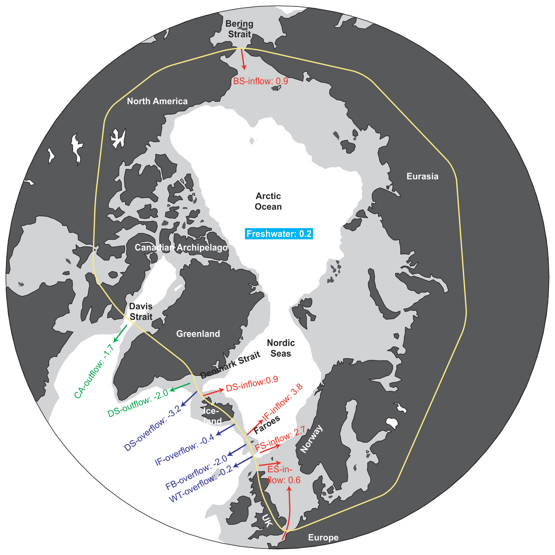
Figure 1The Arctic Mediterranean (roughly represented by the oceanic areas within the yellow curve) and its exchanges with the rest of the World Ocean. Land areas are black. Ocean areas shallower than 1000 m are light grey. Red arrows indicate inflow branches. Dark blue arrows indicate overflow branches. Green arrows indicate surface outflow branches. Labels for arrows refer to Sect. 2 with numbers indicating average volume transport in Sv (1 Sv =106 m3 s−1) based on Table 1.
The inflowing water from the Atlantic that does not return as overflow mixes with the Pacific inflow and leaves the AM through the Canadian Arctic Archipelago and Denmark Strait as cold and relatively fresh “surface outflow” (Curry et al., 2014; de Steur et al., 2017).
Exchanges between the AM and the rest of the World Ocean can therefore be grouped into three types of flow that play important, but different, roles in the ocean and climate systems: inflowof water from the Atlantic and Pacific into the AM, overflowof dense water at depth from the AM into the Atlantic, and surface outflowin the upper layers into the Atlantic (Fig. 2). In addition to these oceanic exchange flows, freshwater enters the AM as runoff, Greenland meltwater discharge, and through net precipitation (Aagaard and Carmack, 1989; Serreze et al., 2006). Ice exports are not considered here as the volume transports are low (same citations).
The important role of the AM in the World Ocean circulation and global climate has been recognized for a long time. There have been many attempts to quantify the AM exchanges and establish a budget for the AM since the pioneering attempt by Worthington (1970). Only recently, however, has the observational coverage become sufficiently comprehensive and reliable that a consistent budget may be determined with confidence.
The flows into and out of the AM are an integral part of the AMOC, which is projected to weaken during the 21st century (IPCC, 2013), and we discuss whether the observations show any indication of this.
In terms of area and volume, the AM is dominated by the Arctic Ocean, for which a budget was proposed by Beszczynska-Möller et al. (2011). Much of the water mass transformation and recirculation within the AM occurs, however, in the Nordic Seas (Mauritzen, 1996). A budget for the whole of the AM, which we try to establish here, will therefore be different from a purely Arctic Ocean budget.
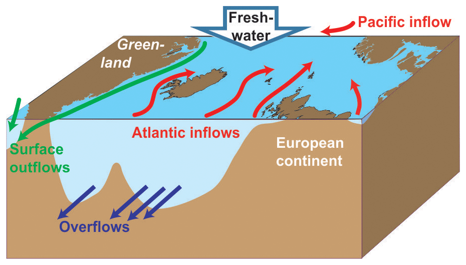
Figure 2In this study, the oceanic flows into and out of the AM are grouped into three categories: inflows, overflows, and (surface) outflows. In addition, rivers, Greenland meltwater discharge, and net ocean surface precipitation supply freshwater to the AM.
In the following sections, we first list the main features and observational systems for each individual exchange branch and the data sets that we use. The combined results of these data are given in Sect. 3 with the main focus on multi-year average transports, seasonal variations, and long-term trends. These results are discussed in Sect. 4, where we initially try to assess whether the combined data set is consistent – e.g. do the combined average transports and their seasonal variations conserve mass. After that, we discuss what is perhaps the most important question of this study: are the total flows into and out of the AM strengthening, weakening, or stable over the time period covered by our observations? The paper ends with Sect. 5 where we present our main conclusions and recommendations.
In this section, we outline the main features of each individual exchange branch and of the observational systems used to quantify and monitor these exchanges. Following tradition (e.g. Hansen and Østerhus, 2000), we group them into the four (including freshwater) categories illustrated in Fig. 2. The distinction between overflows and surface outflows is difficult, especially in the Denmark Strait where they flow together, and will be discussed later (Sects. 2.2.1 and 2.3.2). Here, we use the following well-established criterion: σθ > 27.8 kg m−3 to define overflow (e.g. Dickson and Brown, 1994).
The observational evidence from the individual exchange branches is highly variable. For some branches, we have time series of monthly averaged volume transport spanning more than two decades, although in some cases with gaps. For other branches, the time series are much shorter, or the observational evidence may be barely sufficient to provide one number for the average transport without yielding any information on temporal variations.
To keep the text within readable limits, the descriptions provided in this section do not give complete information about each individual branch. Instead, our aim has been to provide enough information to place each branch as a part of the whole exchange system and describe the observing methodology. For each branch, we list a few key references for access to more detailed information. Where essential details are not available in the literature, we have added information in the Supplement.
2.1 Inflows
Most of the water entering the AM comes from the Atlantic Ocean (Atlantic inflow). The three main Atlantic inflow branches pass through the deep passages across the Greenland–Scotland Ridge (Fig. 3), which are discussed separately. The remaining Atlantic inflows that we also have to consider are the inflows over the Scottish shelf and through the English Channel. Here we combine these two flows into a “European Shelf Atlantic inflow”. Additionally, water from the Pacific Ocean (Pacific inflow) enters the AM through the Bering Strait.
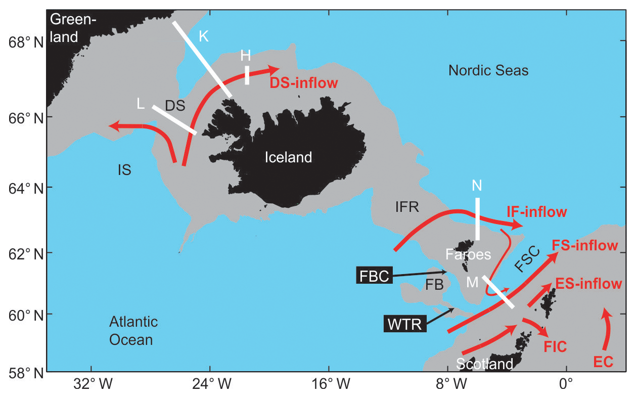
Figure 3The Greenland–Scotland Ridge. Grey areas are shallower than 750 m. Red arrows show schematic flow patterns of the four Atlantic inflow branches. Thick white lines indicate monitoring sections with labels referred to in the text (Sect. 2.1). Topographic features indicated are the Denmark Strait (DS), Irminger Sea (IS), Iceland–Faroe Ridge (IFR), Faroe Bank (FB), Faroe Bank Channel (FBC), Faroe–Shetland Channel (FSC), and Wyville Thomson Ridge (WTR). “ES-inflow” includes contributions from the Fair Isle Current (FIC) and the inflow through the English Channel (EC).
2.1.1 Denmark Strait Atlantic inflow (“DS-inflow”)
The Denmark Strait, between Greenland and Iceland, is about 300 km wide with a sill depth of 630 m. Within the strait, Atlantic water flows towards the Iceland Sea mostly over the Icelandic shelf. The Atlantic inflow passes northwards with the surface Irminger Current along the west coast of Iceland. When it reaches the Denmark Strait it splits into two branches with most of the water not flowing through the strait but flowing west across the Irminger Sea towards Greenland and subsequently southwestwards along the East Greenland continental slope. The other branch flows through the Denmark Strait into the Iceland Sea and continues onto the North Icelandic shelf where it flows eastwards along the shelf as the North Icelandic Irminger Current (Stefánsson, 1962).
The method used for calculating the water mass composition on the Hornbanki section (H section, Fig. 3) and the transport of Atlantic water is described in detail by Jónsson and Valdimarsson (2005, 2016). We use CTD (conductivity–temperature–depth) profiles from the Látrabjarg and Kögur standard sections that have typically been sampled 4 times annually for the period when moorings were present on the Hornbanki section (L and K sections, respectively, Fig. 3). A station on the L section that always lies within the Atlantic water flowing northwards and a station on the K section that is within the Polar waters of the East Greenland Current are combined with temperature measurements from the Hornbanki mooring array (H section, Fig. 3) to calculate the water mass composition at the H section, assuming that it is a mixture of Atlantic and Polar waters. The current-meter records from the H section are then used to calculate the transport of Atlantic water to the AM through the Denmark Strait. The current-meter measurements started in 1994 and have been maintained and made more extensive since then (Jónsson and Valdimarsson, 2012). In 1999 the array was extended from one mooring to three moorings and in 2012 a mooring was added north of the previous moorings. From 1994 to 2009, velocity at the H section was measured with single-point current meters, but starting in 2009 velocity measurements have been made mostly with acoustic Doppler current profilers (ADCPs). There are several gaps in the individual current-meter records probably due to fishing activity in the area and occasional icebergs, but the transport record is continuous since some of the moorings have always been recovered.
The time series for DS-inflow volume transport used in this study consists of monthly averages from October 1994 to December 2015.
2.1.2 Iceland–Faroe Atlantic inflow (“IF-inflow”)
Between Iceland and the Faroes, the Iceland–Faroe Ridge has a sill depth around 480 m close to the Faroes, and is deeper than 300 m over much of its extent. Across this ridge, there is an inflow of Atlantic water to the Nordic Seas in the upper layers (“IF-inflow”), whereas (southward flowing) overflow water crosses the ridge in the opposite direction at depth. Both exchanges occur over most of the length of the ridge, but likely with large temporal and spatial variations (Tait, 1967; Meincke, 1983; Perkins et al., 1998; Rossby et al., 2009, 2018). Due to the high spatial and temporal variability of these exchanges, a monitoring array located on the ridge that could generate time series of IF-inflow volume transport would need to be very extensive and would be vulnerable to the intensive fishing activity. This has not been attempted.
Instead, monitoring has been established on a section (the N section, Fig. 3) east of the ridge where the inflow crossing the ridge is focused into a relatively narrow boundary current, the Faroe Current, which includes all the Atlantic water entering the AM in this region. This current flows eastwards north of the Faroes, bounded on the north side by the Iceland–Faroe Front (Tait, 1967; Hansen and Meincke, 1979; Read and Pollard, 1992). The N section has been sampled 3–4 times annually by CTD cruises since the late 1980s. Since 1997, this has been complemented by an array of moored ADCPs, deployed below the extent of fishing gear or in trawl-protected frames on the bottom. Based on the combined ADCP and CTD data, Hansen et al. (2003) derived average estimates and time series of volume transport for the IF-inflow, representing the Atlantic water crossing the ridge.
The volume transport based solely on in situ observations was found to be well correlated with the sea level tilt on the section derived from altimetry data (Hansen et al., 2010), and a new algorithm was developed which combines data from altimetry and in situ observations (Hansen et al., 2015). Based on this, the time series for IF-inflow volume transport used in this study consists of monthly averages from January 1993 to December 2015.
2.1.3 Faroe–Shetland Atlantic inflow (“FS-inflow”)
The gap in the Greenland–Scotland Ridge between the Faroes and Scotland is called the Faroe–Shetland Channel (FSC). The deepest part of the channel is deeper than 1000 m. Water of Atlantic origin usually fills the upper layers down to 400–500 m across the whole channel, but a significant fraction of that water originally crossed the ridge north of the Faroes, entered the Faroe Current, and bifurcated into the FSC, where it flows southwestwards along the Faroe side of the channel (Fig. 3; Helland-Hansen and Nansen, 1909; Meincke, 1978; Hátún, 2004; Berx et al., 2013). Most of this water is believed to recirculate within the channel and join the direct inflow continuing into the Norwegian Sea (Hansen et al., 2017).
Regular hydrographic surveys along standard sections crossing the channel have been carried out for more than a century (Tait, 1957; Turrell, 1995) and, since the 1970s, these have been complemented with current-meter moorings and other instrumentation (Gould et al., 1985; Dooley and Meincke, 1981; Rossby and Flagg, 2012; Berx et al., 2013; Rossby et al., 2018). In this study, we use data from the only long-term transport monitoring effort (Østerhus et al., 2001), consisting of CTD profiles and moored ADCP time series along a standard section (the Munken–Fair Isle section, labelled M in Fig. 3) starting in 1994. The recirculation of Atlantic water and intensive mesoscale activity (Sherwin et al., 1999, 2006; Chafik, 2012) complicate the calculation of volume transport. By combining the in situ observations with data from satellite altimetry, Berx et al. (2013) generated a time series of volume transport of the FS-inflow with monthly estimates from January 1993 to September 2011, here extended to December 2015.
The time series generated by Berx et al. (2013) represents the Atlantic water flow between the shelf edges on both sides of the channel. On the Faroe shelf, northwest of the shelf edge boundary of the channel, there is a flow between the islands and the shelf edge, which generally is directed southwestwards. Most of this is considered to belong to a quasi-closed shelf circulation around the Faroes (Larsen et al., 2008) and therefore is not advected into the AM. This shelf circulation is not included in the IF-inflow as it passes eastwards north of the Faroes (Hansen et al., 2003) and should therefore not be included in the FSC either. For the continental shelf region southeast of the FSC monitoring section, there is, on the other hand, an Atlantic inflow, which is not recirculated around the UK. That contribution is discussed in the next section, Sect. 2.1.4.
2.1.4 European Shelf Atlantic inflow (“ES-inflow”)
The European Shelf (ES)-inflow is the inflow of Atlantic water between the southeastern boundary of the Faroe–Shetland Channel monitoring system and the European continent. The previously discussed (Sect. 2.1.3) Atlantic water flow through the channel – the FS-inflow – has been monitored on a section (the M section in Fig. 3) that terminates at a point just inside the shelf edge on the Scottish shelf with bottom depth of ∼150 m (Berx et al., 2013; bottom right extent of white line in Fig. 3). Between this point and the Orkneys, there is a distance of ∼125 km (which we call here the Scottish shelf), through which there may be appreciable flow. Unfortunately, this has not been systematically monitored and observationally based estimates of its volume transport seem difficult to find.
Despite this lack of observational evidence, the average volume transport over the Scottish shelf must at least be equal to the average volume transport of the Fair Isle Current that passes into the North Sea through the gap between the Orkneys and Shetland – the Fair Isle Gap (Fig. 3). This current was estimated by Turrell et al. (1990) to have an average transport of 0.13 Sv. Their observations only covered a few months, however, and Hill et al. (2008) have updated this value to 0.4 Sv, based on a combined observational and modelling effort.
This value may thus represent a minimum average volume transport over the Scottish shelf, but some of the water over the shelf may continue northeastwards to flow west of Shetland rather than passing through the Fair Isle Gap. Again, there is little observational evidence, but some information may be gained from measurements by a ferry-mounted ADCP (Rossby and Flagg, 2012). The focus of the ADCP data acquisition was on larger scales; but from their graphs and updated graphs reported by Childers et al. (2014), we estimate an additional ∼0.1 Sv of water flowing into the AM, giving a total average volume transport of 0.5 Sv over the Scottish shelf inside of the M section.
The flows over the Scottish shelf and through the English Channel include less saline water from coastal areas upstream in addition to the more oceanic component. Thus, the term “Atlantic” may be somewhat misleading but, for our purpose, it is the total volume transport rather than the characteristics of the water that is important. These coastal water masses are therefore included in the ES-inflow.
From in situ observations, there is little evidence about the variations in volume transport, but satellite altimetry may be used for that purpose as long as we can assume geostrophy, which works well for the neighbouring FS-inflow (Berx et al., 2013). As elaborated on in the Supplement, we have therefore combined the established average transport value with sea level anomalies (SLA values) from altimetry to generate monthly time series of ES-inflow with the additional assumption of barotropic flow. This assumption probably leads to transport variations that are too high, but they are still low in absolute terms and should not have much influence on the overall picture.
In addition to the flow over the Scottish shelf, there is also an inflow of Atlantic water through the English Channel, which according to the observations reported by Prandle (1993) has an average volume transport of ∼0.1 Sv. Altogether, we will therefore use a value of (0.6±0.2) Sv for the average volume transport of the ES-inflow where the uncertainty value is estimated from the limited observational evidence.
2.1.5 Bering Strait Pacific inflow (“BS-inflow”)
The Bering Strait is a narrow (width ∼85 km) and shallow (sill depth ∼50 m) strait connecting the Pacific and Arctic oceans (Fig. 4). Since 1990, year-round measurements have been maintained in the strait almost without interruption, typically at 2–3 sites (Fig. 4) located within one or both of the two channels of the strait (sites A1 and A2), and typically also at a mid-strait site, A3, slightly to the north, at a location found to give a useful average of the flows from the two channels (e.g. see Woodgate et al., 2015, for discussion). In 2001, a mooring (A4) was added in the eastern side of the eastern channel to monitor the warm low-salinity Alaskan Coastal Current (ACC) present seasonally (Woodgate et al., 2015).
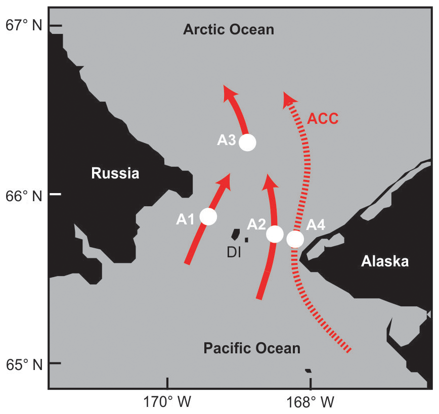
Figure 4The Bering Strait has two channels separated by the Diomede Islands (DI). Red arrows indicate annual mean flow paths. White circles mark mooring positions (A1, A2, A3, A4). Dashed arrow marks the Alaskan Coastal Current (ACC), present seasonally. Grey areas are shallower than 100 m.
In the 1990s, velocities at the mooring sites were measured mostly by single-point current meters; but since 2007, velocity measurements have been made predominantly with ADCPs. Based on the observed dominantly barotropic and spatially homogeneous nature of the flow (away from the ACC), volume transport is calculated by multiplication of velocity and cross-sectional area for the strait (Woodgate, 2018).
Over the period of monitoring (1990 to present), there has been a statistically significant increase in annually averaged volume transport from 0.8 Sv in the beginning of the period (Roach et al., 1995) to ∼1.2 Sv by the end (Woodgate, 2018). Here, we use the monthly mean volume transports from August 1997 to December 2013.
2.2 Overflows
The only deep connections between the AM and the rest of the World Ocean are the gaps in the Greenland–Scotland Ridge and only through these gaps do we find the flows of dense water from the AM that are generally characterized as “overflow”. In the literature, various criteria have been used to define overflow – either in terms of temperature or density. In this study, we use the most common definition that σθ > 27.8 kg m−3 (e.g. Dickson and Brown, 1994). We also follow common practice (e.g. Hansen and Østerhus, 2000) to group the overflow into four different branches (Fig. 5).
2.2.1 Denmark Strait overflow (“DS-overflow”)
About half of the dense overflow waters from the Nordic Seas enter the North Atlantic through Denmark Strait, where the DS-overflow becomes one of the major sources of NADW (e.g. Dickson and Brown, 1994). The overflow plume crossing the passage between Iceland and Greenland is generally found at a depth below 250 m, although close to the Icelandic shelf warm and saline Atlantic water frequently occupies the passage down to the bottom (Mastropole et al., 2017).
The width of the Denmark Strait, which is deeper than 350 m, covers a distance of 60 km only. Here, the overflow plume is most intense with downstream velocities exceeding 1 m s−1 and near-bottom temperatures below 0 ∘C. Mesoscale eddy activity is well documented, and occurs with periods of 2–10 days (Ross, 1984; Käse et al., 2003; Fischer et al., 2015), whereas seasonal variability is small and no significant long-term trends have been found so far (Jochumsen et al., 2012). Moored instrumentation for current profile measurements (ADCPs) have been installed in this part of the passage (the L section in Fig. 5). The standard deployment consists of two moorings: one at 650 m depth at the deepest part of the sill of the strait, the other 10 km further towards Greenland at 570 m depth. These positions cover the overflow current core, but a large volume of dense water on the Greenland shelf is not accounted for.

Figure 5Overflow and surface outflow branches across the Greenland–Scotland Ridge. Grey area is shallower than 750 m. Arrows indicate schematic flow patterns of the four overflow branches (dark blue, discussed in Sect. 2.2) and the one surface outflow across the ridge (green, discussed in Sect. 2.3). Thick white lines indicate monitoring sections with labels referred to in the text. Topographic features indicated are Iceland–Faroe Ridge (IFR), Faroe–Shetland Channel (FSC), and Western Valley (WV).
Velocities on the shelf are small, but the distance to the coast of Greenland is still more than 250 km, where some dense water is transported southward (de Steur et al., 2017). In earlier publications, this transport was inferred from a model and added to the transport calculations obtained by the moorings (Macrander et al., 2005; Jochumsen et al., 2012). In 2014/2015, however, an experiment was made with five moorings on the L section, from which a new algorithm was developed to derive volume transport from the historical ADCPs observations (Jochumsen et al., 2017). The monthly averaged DS-overflow transport values used here are based on this algorithm and extend from May 1996 to December 2015, although with gaps.
A quality check on this new time series is provided by the experiment reported by Harden et al. (2016) with a dense mooring array on the K section (Fig. 5) lasting from September 2011 to July 2012. For the overlapping period (336 days), our data set based on Jochumsen et al. (2017) has an average transport of 3.1 Sv, whereas Harden et al. (2016) find 3.5 Sv. Considering the uncertainties reported (±0.5) and possible water mass transformations between the two sections, this comparison is encouraging (Jochumsen et al., 2017).
2.2.2 Iceland–Faroe Ridge overflow (“IF-overflow”)
Overflow across the Iceland–Faroe Ridge was identified more than a century ago (Knudsen, 1898) and it has long been known that it may occur at many locations along the ridge (Hermann, 1967; Meincke, 1983). From the results of the “Overflow ′60” expedition, Hermann (1967) estimated a total volume transport of 1.1 Sv for the IF-overflow. Based on moorings and hydrographic observations, Perkins et al. (1998) estimated at least 0.7 Sv overflow close to Iceland, and Beaird et al. (2013) used measurements from autonomous Seagliders to find a minimum of 0.8 Sv for the total overflow across the ridge. However, observationally based information on temporal variations or time series of total IF-overflow have not been published.
The Iceland–Faroe Ridge may conveniently be divided into two parts at the latitude of 63∘ N (Fig. 5). Across the southern (Faroese) part, the overflow is considered to be intermittent (Østerhus et al., 2008) and from their extensive Seaglider experiment, Beaird et al. (2013) estimated an average volume transport of that part of the overflow of 0.3 Sv with an uncertainty almost as high.
Across the northern (Icelandic) part, the overflow has generally been thought to be more persistent (Østerhus et al., 2008), especially the overflow through the northernmost passage across the ridge, labelled the Western Valley (Fig. 5). This is partly from theoretical arguments and partly from observations of a strong and persistent bottom current downstream from the Western Valley that seems to have been generated by IF-overflow (Perkins et al., 1998; Olsen et al., 2016). Measurements within the Western Valley have not, however, shown any clear evidence of strong overflow (Perkins et al., 1998; Beaird et al., 2013); and based on a dedicated field experiment from August 2016 to May 2017, Hansen et al. (2018) argue that the long-term average overflow transport through the Western Valley is less than 0.1 Sv.
Following these recent results, we use 0.4 Sv for the average transport of IF-overflow with an uncertainty of ±0.3 Sv. This quantity for the average transport may seem small when the bottom current downstream of the Western Valley is taken into account (Perkins et al., 1998; Olsen et al., 2016), but the volume transport of this current is not well constrained by observations and neither are its origin and en-route entrainment of Atlantic water. From bottom temperature measurements (Olsen et al., 2016), it also seems unlikely that much of this water would fulfil the criterion for overflow. Seasonal and long-term variations in the IF-overflow cannot be addressed with the observational material available.
2.2.3 Faroe Bank Channel overflow (“FB-overflow”)
The Faroe Bank Channel is the deepest passage across the Greenland–Scotland Ridge with a sill depth of 840 m. The bottom layer in this channel is continually dominated by cold overflow water that flows over the sill with core speed usually exceeding 1 m s−1 out into the Atlantic (Hermann, 1959; Borenäs and Lundberg, 1988; Saunders, 2001; Hansen and Østerhus, 2007; Hansen et al., 2016).
Since the early estimates by Hermann (1967) and Sætre (1967), several transport estimates for the FB-overflow have been published. Here, we use the most comprehensive data set consisting of data from long-term ADCP moorings on the V section (Fig. 5), combined with other moored instrumentation and regular CTD cruises (Hansen et al., 2016). The primary time series generated from these observations is the “kinematic overflow”, which is based on velocity (ADCP) measurements alone. This time series has an average volume transport of 2.1 Sv, which, however, includes 0.2 Sv of water less dense than the established criterion (σθ≥27.8 kg m−3). For our purpose, the time series has therefore been converted by multiplying the values with a fixed ratio of (2.1–0.2)/2.1. The series contains monthly averaged volume transport from December 1995 to December 2015, although with gaps during the annual servicing periods.
2.2.4 Wyville Thomson Ridge overflow (“WT-overflow”)
The Wyville Thomson Ridge has a sill depth of around 600 m with intermittent overflow of dense water both at the deepest point at the centre of the ridge and at the far west of the ridge (Ellett and Roberts, 1973; Sherwin et al., 2008; Johnson et al., 2017). This flow, the WT-overflow, is channelled by topography into the Ellett Gully before entering the Rockall Trough to the south. The flow through the Ellett Gully has primarily been monitored by ADCP moorings but also by a CTD section (the W section in Fig. 5).
The time-varying nature of WT-overflow necessitates the combination of volume transports with proportions of Faroe–Shetland Channel Bottom Water (FSCBW) in order to produce a transport comparable to other overflow time series (Sherwin et al., 2008). In this method, the volume transport through the Ellett Gulley, as measured by the moored ADCP, is weighted by the proportion of FSCBW in the water column, calculated from linear mixing between FSCBW (defined as having a temperature of 0 ∘C) and Atlantic Water (defined as having a temperature of 8.5 ∘C). The method assumes temperature decreases linearly from the depth of the 8.5 ∘C isotherm to the seabed, and that the isotherms are horizontal. Sensitivity tests suggest that the error associated with these assumptions is less than ±20 % (±0.04 Sv). The time series of WT-overflow used in this study is based on this method and consists of monthly averages from May 2006 to May 2013, although there is a data gap from June 2009 to May 2011 due to instrument loss.
The definition of FSCBW is slightly denser than our criterion for overflow water (27.8 kg m−3) and thus 0.2 Sv is a lower bound for the volume transport. Previous measurements in the region have suggested transports between 0.1 and 0.3 Sv (Hansen and Østerhus, 2000). We therefore use the time series of WT-overflow transport based on the method of Sherwin et al. (2008) but attach an uncertainty of ±0.1 Sv.
2.3 Surface outflows
In addition to the overflow of dense water through the deep passages across the Greenland–Scotland Ridge, the AM also exports water that is less dense and remains in the upper layers. The flow of these water masses is denoted as “surface outflow” or just “outflow” and it may be seen as two separate branches passing on either side of Greenland.
2.3.1 Canadian Arctic Archipelago surface outflow (“CA-outflow”)
The Canadian Arctic Archipelago (CAA) is a collection of numerous islands separated by narrow sounds. Through these sounds and through the Nares Strait, separating the CAA from Greenland, there is a net flow of water from the Arctic Ocean towards the Labrador Sea (Fig. 6). Measurements of these flows are difficult due to ice, strong tidal currents, recirculation, and proximity to the magnetic pole. Nevertheless, volume transport has been estimated from observations at several locations (Melling et al., 2008).

Figure 6Outflow from the Arctic Ocean through the Canadian Arctic Archipelago. Flows through Nares Strait (NS), Jones Sound (JS), Lancaster Sound (LS), and Fury and Hecla Strait (FHS) as well as the Baffin Island Current (BIC) are indicated by blue arrows. The thick white line indicates the Davis Strait monitoring section. Red arrows indicate water flowing northwards through the section before recirculating, joining, and partly mixing with the Arctic Ocean outflow and exiting south again. Grey areas on the map are shallower than 1000 m.
Davis Strait connects Baffin Bay to the Labrador Sea and has a sill (640 m depth) that limits deep exchanges between the two. Exchanges through the strait are predominantly two way and topographically steered (Tang et al., 2004). Southward flow, on the western side of Davis Strait, carries inputs from the integrated CAA through flows. Northward flow, on the eastern side of the strait, consists of the low-salinity West Greenland Current (WGC) on the shelf and the warm, salty West Greenland Slope Current (WGSC) of North Atlantic origin over the slope (Curry et al., 2014). The WGC is a combination of the East Greenland Current (EGC) flowing southward from the Arctic through Fram Strait (de Steur et al., 2009) and the East Greenland Coastal Current (EGCC) arising from the addition of East Greenland coastal inflow and glacial runoff (Bacon et al., 2002; Sutherland and Pickart, 2008). The WGSC is a branch of the North Atlantic Current that enters and circulates cyclonically in the Irminger Sea and continues along the East Greenland slope seaward of the EGC around Greenland (Cuny et al., 2002; Myers et al., 2007). Both the WGC and WGSC flow around the southern tip of Greenland and then turn north toward Baffin Bay. Transport through Davis Strait has been monitored using a mooring array north of the sill that includes velocity, temperature, and salinity measurements from 15 moorings spanning the full width (330 km) of the strait accompanied by autonomous Seaglider surveys (Curry et al., 2014).
Transport through Davis Strait is used to represent the CA-outflow in this study. We use monthly averaged volume transports from October 2004 to September 2010. There is a small component of the Arctic Ocean outflow that bypasses Baffin Bay and flows through Fury and Hecla Strait (Fig. 6). Its volume transport is not well constrained but has been estimated to be less than 0.1 Sv (Straneo and Saucier, 2008). It will not be included here.
2.3.2 Denmark Strait surface outflow (“DS-outflow”)
The surface outflow through the Denmark Strait is difficult to monitor. At times it may flow through a large part of the width of the strait, requiring a wide and dense mooring array while the component flowing over the East Greenland shelf is inundated with icebergs that are very destructive to moored instrumentation. It therefore comes as no surprise that observation-based transport values of the DS-outflow have been late to arrive.
The values used here are mainly based on the experiment described in Sect. 2.2.1 with a dense mooring array along the K section (Fig. 5) from September 2011 to July 2012 (Harden et al., 2016). There, the focus was on the dense-water component (σθ > 27.8 kg m−3), but the transport of the less dense water masses (σθ < 27.8 kg m−3) could also be derived from the observations as reported by de Steur et al. (2017). They estimated the average transport of this upper-ocean component to be 1.8 Sv towards the southwest with an uncertainty of the order of ±0.5 Sv. This value does not, however, cover the East Greenland shelf region adequately.
To amend this, we add data from additional inshore moorings on the K section from 2012 to 2014 reported by de Steur et al. (2017). From these additional data, monthly averages of the transport over the shelf can be generated, and we add these to the monthly averages from the 2011–2012 experiment (Fig. 9b in de Steur et al., 2017). In this way, we obtain a time series of 11 months from September 2011 to July 2012, which should include the total surface outflow through the Denmark Strait. The validity of this approach is of course dependent on the stationarity of the seasonal cycle over the shelf, which is questionable, but the modification due to the addition of the 2012–2014 inshore moorings is small.
On this basis, we have estimated a value of 2.0 Sv for the average DS-outflow. This value is composed of two non-concurrent contributions, the dominant of which was based on only 11 months of observations. It must therefore be treated with caution, as must the seasonal variation indicated by the data, which shows a pronounced winter-intensification of the DS-outflow. A strong seasonality of the flow over the Greenland slope is, however, supported by more prolonged current measurements in this region (Jónsson, 1999). The transport of the East Greenland Current at 74∘ N was also found to be subject to a large seasonal cycle related to the wind-driven gyre in the Greenland Sea (Woodgate et al., 1999).
2.4 Runoff and precipitation (“Freshwater input”)
In addition to oceanic inflows, water enters the AM by net precipitation (precipitation minus evaporation) and runoff from rivers as well as land-ice melting into the sea, which we consider collectively as “Freshwater input”. Since the various freshwater contributions have relatively small magnitudes, they are commonly reported in millisverdrup (mSv where 1 mSv Sv).
The freshwater budget of the Arctic Ocean was pioneered by Aagaard and Carmack (1989) and updated by Serreze et al. (2006) who reported a net precipitation of 65 mSv and a runoff of 102 mSv to the Arctic Ocean. Including also the Nordic Seas, Dickson et al. (2007) added 20 mSv of net precipitation and 34 mSv of runoff from the Baltic, the Norwegian coast, and Greenland. Another 9 mSv enter the Canadian Arctic Archipelago from Greenland according to Dickson et al. (2007). This yields a total freshwater input to the traditional AM of 230 mSv, which we round to 0.2 Sv with an estimated uncertainty less than 0.1 Sv. Since we also include the North Sea in our definition of the AM (Fig. 1), there are additional inputs, especially river runoff from Belgium, the Netherlands, and Germany into the North Sea, but they are only a few millisverdrup and too small to affect this value (Radach and Pätsch, 2007).
Most of the freshwater contributions exhibit strong seasonality. According to Serreze et al. (2006), the net precipitation to the Arctic Ocean is more than twice as high in July as in March and river runoff to the Arctic Ocean has an even more pronounced seasonal variation. A similar, although less extreme, seasonal variation has been reported for river runoff to the Baltic (Bergström and Carlsson, 1994). Within the uncertainties generally applying to this study, it therefore seems safe to assume a seasonal variation of Freshwater input to the AM with amplitude around 0.1 Sv and maximum around July.
In addition to seasonal, there are also long-term variations and Haine et al. (2015) suggest that net precipitation and runoff to the Arctic Ocean and Canadian Arctic Archipelago were greater in the 2000s than for 1980–2000. The observational evidence for this is, however, weak and in any case within the quoted uncertainty. Thus, it will be ignored here.
Table 1Observational characteristics of each AM-exchange branch. The full period of observations is listed with the number of months observed (Months) and the number of missing months (Gaps). The uncertainties of the average values are based on the information in Sect. 2. The average transport values (Avg.) are positive into the AM and negative out of the AM. SD is the standard deviation of the monthly averages. References to the sources for the data are listed for each branch in Sect. 2. For IF-overflow and Freshwater, time series are not available (NA).
As described in the previous section, monthly transport values are available for almost all of the oceanic exchange branches into or out of the AM, although of highly variable duration and completeness. These monthly averaged values (ignoring the fact that months have different number of days) are the basic data set used in this study (Table 1). The one exception is the IF-overflow that has not been systematically monitored and for which we only have estimated a typical or “average” transport value and its uncertainty. Likewise, for the Freshwater input we only have an average value and a seasonal amplitude. In the following, we present the average transports, as determined from the various data sets (over differing time-periods), as well as their variations on seasonal and long-term timescales. Transport values are defined as positive into the AM and negative out of the AM.
3.1 Average volume transports
Combining all the inflow transports with the freshwater input, we get the total “AM-import”, which has an average value of 9.1 Sv. Likewise, we can combine all the overflow transports with the surface outflow transports to an “AM-export” with an average value of −9.5 Sv. Hence, the export exceeds the import so that the average Net import (AM import + AM export) is −0.4 Sv. Combining the various uncertainty terms, this number has an uncertainty exceeding 1 Sv.
Thus, the imbalance in the average Net import is within the combined uncertainties even though the various numbers in Table 1 are averaged over widely different periods. The most complete coverage is during a 6-year period, from October 2004 to September 2010, in which there are 53 months with data from all of the inflow branches, from the DS-overflow, the FB-overflow, and from the CA-outflow. The sum of the transport values for all of these branches in these months are all inside the error estimate for the sum based on the full periods (Table 1).
3.2 Seasonal variation
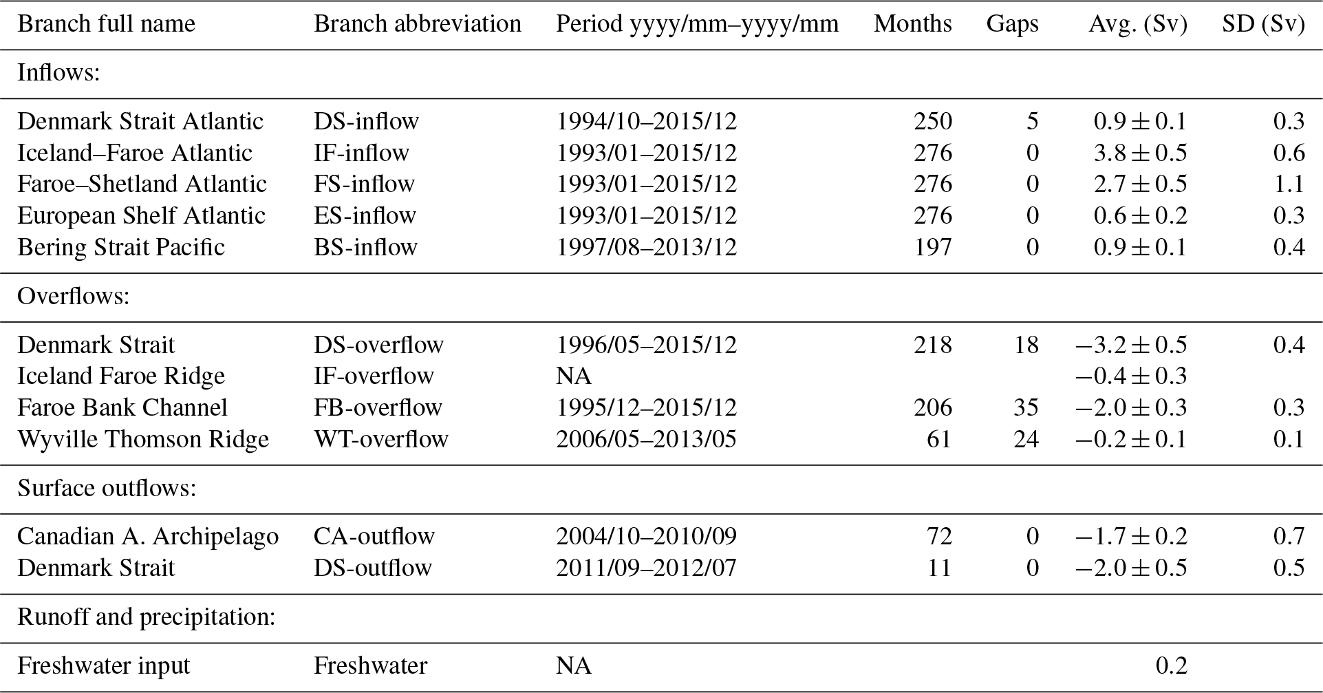
Table 1 also lists the standard deviation of the monthly transport values for each individual branch and some branches are clearly more variable than others, especially when considering the ratio between standard deviation and average transport. Thus, the monthly standard deviation of the FS-inflow is almost twice that of the IF-inflow even though the IF-inflow has a higher average transport.
Some of this variability seems to derive from systematic seasonal variations as indicated in Fig. 7, where we have compared seasonal variations during the most complete 6-year period. The inflow branches seem to have different seasonal variations (Fig. 7a), with the IF-inflow, the FS-inflow, and the ES-inflow being strongest around the turn of the year, whereas the BS-inflow and the DS-inflow are strongest in summer. For the overflow and surface outflow branches, the picture seems less clear (Fig. 7b) and most of the export branches do not exhibit any clear seasonality.
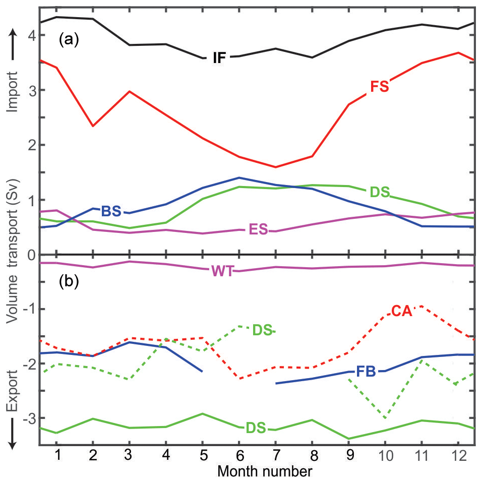
Figure 7Seasonal variation in five inflow branches (a), three overflow branches (continuous lines in b), and two surface outflow branches (dashed lines in b). All the lines are based on observations taken between October 2004 and September 2010 except for the DS-outflow (dashed green line in b), which is based on the September 2011 to July 2012 period with inshore values from 2013 to 2014 (Sect. 2.3.2). We have no seasonal information for the IF-overflow and so it is not included in this plot. See Table 1 for abbreviations.
To get a more complete impression of the seasonal variation, the monthly transport values for the five inflow branches in Fig. 7a have been summed to give the total AM import when the Freshwater input is neglected. Subtracting the overall average, we get the seasonal import anomaly, which is shown as the red curve in Fig. 8. Similarly, the blue curve in that figure shows the seasonal anomaly of the AM export; although note that this neglects the IF-overflow and missing months for the FB-overflow and DS-outflow that had to be interpolated to get a complete seasonal coverage.
Combining the red and blue curves in Fig. 8, we get the seasonal anomaly of the Net import for those branches that have been sufficiently well observed (black curve). It seems to indicate a maximum in November and minimum in August with an amplitude of the order of 1 Sv. A more detailed discussion of this imbalance will be presented in Sect. 4.2, but it is worth emphasizing that this curve is not based on a very homogeneous data set. The inflow branches and the CA-outflow had no gaps in the selected period, but that was not the case for the overflow branches and our data for the DS-outflow only cover 11 months and they are outside the selected period.
3.3 Long-term variations
Only the five inflow branches and the two main overflow branches have been observed over sufficiently long periods to allow a meaningful investigation of possible long-term variations or trends. The FB-overflow has months missing for almost every year but for the other branches, annual averages may be computed for most of the years within the observing period. Based on these annual averages, Table 2 lists linear trends as calculated by linear regression of annual volume transport over time.
Table 2Linear trends of annual averages of the five inflow branches individually and summed and of the DS-overflow. Only years with complete coverage (no months missing) are included and the number of years is listed. The trend is represented by its value ± its 95 % confidence interval. Branches with trends that are significant at the 95 % level are marked in bold. The last column lists relative trends (Rel. tr.) determined by dividing the trends with the average transports from Table 1.
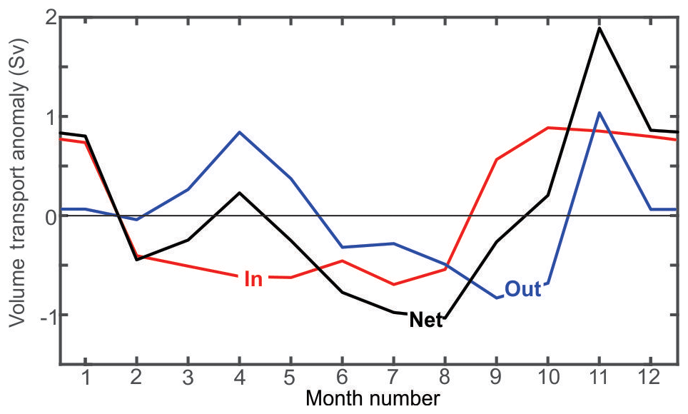
Figure 8Seasonal anomalies of the combined inflow branches (red) and the combined overflow and surface outflow branches (blue) for the same periods as in Fig. 8, where missing months have been interpolated. The black curve is the sum of the other two curves and represents the anomaly of the Net import when the IF-overflow (order 0.4 Sv in the annual mean) and Freshwater input (order 0.2 Sv in the annual mean) are neglected.
Except for the BS-inflow, the trends in Table 2 are less than their confidence intervals, which are calculated without taking serial correlation (autocorrelation) into account. The number of degrees of freedom are therefore probably too high and thus these confidence intervals are likely to be underestimates of the real uncertainty in the trend. The exchanges between the AM and the Atlantic are therefore characterized by stability rather than change – at least over the observed period.
A more illustrative picture of the long-term variation is presented in Fig. 9, which shows low-pass filtered series generated by averaging all observed months (up to 36) in 3-year periods. For some branches, months were missing for some of the 3-year periods, but never more than 6 months. Thus, all the points in Fig. 9 are averaged over at least 30 months. The curves in Fig. 9 are consistent with Table 2 with only weak trends for most of the branches and relatively small variations.
The longest time series considered here are for the four Atlantic inflow branches and the two main overflow branches. From 1996 to 2015, the Atlantic inflow branches had almost complete coverage and the total volume transport of these branches had at most 2 months missing in every 3-year period. Thus the thick red line in Fig. 10 should give a good representation of the variations of the total Atlantic inflow during these 18 years. The sum of the two main overflow branches has less complete coverage, but the de-seasoned 3-year running mean (thick blue line in Fig. 10) still should give an indication of the variation in this series.
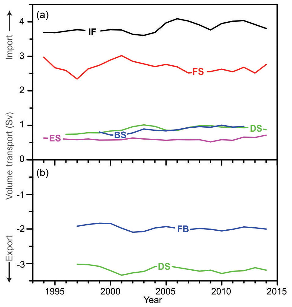
Figure 9Low-pass filtered (3-year running mean) volume transport of the five inflow branches (a) and the two main overflow branches (b). The value for each year is the average of the values for all observed months of the year, the preceding year, and the following year. To minimize bias from missing months, the values have been de-seasoned before averaging (Sect. S2 in the Supplement).
Figure 10 shows the change in inflow/overflow relative to their late 1990s values. For both the total Atlantic inflow and the sum of the two main overflow branches, Fig. 10 seems to indicate strengthening from the late 1990s to 2002 with little overall change after that. When taking the uncertainties (coloured areas in Fig. 10) into account, the statistical significance of the apparent changes seems low, however, and the overall message is one of stability.
The results presented in the previous section are from a wide and inhomogeneous set of observational systems. The first question to ask is therefore whether they are mutually consistent. From Table 1, the estimated AM export is 0.4 Sv higher than the AM import, but this imbalance is well within the uncertainties quoted in the table and needs no further explanation. Whether to expect a zero imbalance in our data set is, however, not as obvious as might be thought and is discussed in Sect. 4.1.
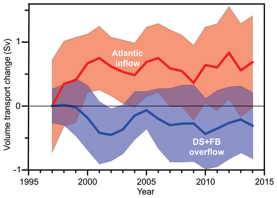
Figure 10Low-pass filtered (3-year running mean) volume transport change (from the value in 1997) of the sum of the four Atlantic inflow branches (thick red line) and the sum of the two main overflow branches (thick blue line). The value for each year is the average of the de-seasoned values for all observed months of the year, the preceding year, and the following year. The coloured areas represent the 95 % confidence interval (Sect. S2).
Similarly, the Net import in our data set appears to have a non-zero seasonal variation (Fig. 8) and we need to ask whether it is within acceptable bounds. The following Sects. 4.1 and 4.2 therefore address what constraints nature puts on the average value and seasonal variation in the net import. Another problem is that the individual observational systems do not combine into a contiguous whole. This is discussed in Sect. 4.3. The implications of the apparent imbalances in our results for data quality are summarized in Sect. 4.4. In a very simplified picture, the AM may be seen as a double estuary with an estuarine as well as a thermohaline loop. In Sect. 4.5, we estimate the relative strengths of these two loops and their sources. After that, in Sect. 4.6, we address the important question: have the total flows into and out of the AM been weakening, strengthening, or remained stable within our observational period?
4.1 Constraints on the average AM-exchange budget
The ultimate criterion for a consistent exchange budget is mass conservation. When there is an imbalance between import and export, the total mass within the AM must change accordingly. If there were no density changes, the mass balance would be equivalent to volume balance (continuity). An imbalance of 0.1 Sv that is sustained for a year would then imply a sea level change around 20 cm on average over the whole AM. This is considerably more than available observations indicate for inter-annual sea level variations (Volkov and Pujol, 2012; Andersen and Piccioni, 2016), although observational evidence is missing for much of the Arctic Ocean. Basin-wide GRACE Ocean Bottom Pressure data suggest interannual trends between 2002 and 2006 of only a few centimetres (< 5 cm yr−1) over the Arctic basin, and of varying sign (Morison et al., 2007); this is further evidence that an imbalance of 0.1 Sv is unrealistic.
In reality, air–sea exchanges and mixing with runoff and other water masses induce density changes in the water between entering and leaving the AM, but they are too small to affect this calculation significantly. In addition to this, the induced expansion and contraction of the water result in steric sea level changes within the AM that add to the mass-induced changes but, again, the inter-annual variations caused by this are considerably smaller than 20 cm in the areas reported (Mork and Skagseth, 2005; Andersen and Piccioni, 2016).
When averaging over a period of a year or longer, the imbalance between AM import and AM export therefore has to be considerably smaller than 0.1 Sv. The imbalance we find in our observational estimates of the import/export are thus almost certainly due to the present limitations of the observational system.
4.2 Constraints on the seasonal AM-exchange variations
For the seasonal variation in transports, mass conservation must again be required but now the implications are more intricate. As a framework for the discussion, consider a model, in which the Net import anomaly (Net import minus its temporal mean), Q(t), varies sinusoidally with time, t:
where Q0 and τQ are the seasonal amplitude and time of maximum for the Net import, respectively, and T is 1 year. Initially, we furthermore assume incompressibility so that there are no density changes and no steric sea level variations. In that case, continuity requires that the sea level height anomaly (sea level height minus its temporal mean) averaged over the whole of the AM, H(t), fulfils
where A is the surface area of the AM and the seasonal amplitude of H(t), H0, and the time of sea level maximum, τH, are given by
Thus, the seasonal amplitude of the Net import, Q0, may be estimated from the seasonal amplitude of the average sea level height, H0, and Q(t) should be at maximum three months (T∕4) before the time of sea level maximum. In reality, the assumption of incompressibility is not valid but this problem can be circumvented by subtracting steric seasonal variations from H(t) before calculating H0 and τH. If we can determine H0 and τH from observations, we can therefore estimate what values Q0 and τQ should have.
In the Nordic Seas, there is fairly good observational evidence of seasonal sea level variations from satellite altimetry. In this region, Mork and Skagseth (2005) found that a sinusoidal variation typically explained 40 %–50 % of the total variance. Over the deep parts, maximum sea level occurred around September with amplitudes between 4 and 8 cm. They furthermore found that the steric component was in phase with the observed total variation and typically contributed around 40 %. These results were validated by Volkov and Pujol (2012) who compared the altimetry data with tide gauge records and also extended the region to include the Barents and Kara seas. Except for near-coastal areas, it seems that when corrected for steric variation, the average value for H0 in this region does not exceed 5 cm and maximum sea level is in autumn.
In the open Arctic Ocean, ice cover and a lack of satellite coverage put severe limits on our knowledge of sea level variations but recently Andersen and Piccioni (2016) have reported an analysis of sea level variation in the region from 66 to 82∘ N, which supports the value of 5 cm as a maximum for H0 in this region. Similarly, Peralta-Ferriz and Morison (2010), find, from GRACE data, a seasonal cycle within the Arctic of ∼5 cm. Combining this information with Eq. (3), we conclude that in nature, the Net import anomaly, Q(t), is maximum in summer and its seasonal amplitude, Q0, does not exceed 0.2 Sv.
The seasonal anomaly of the Net import derived from our data set (black curve in Fig. 8) is not at all consistent with this. In Fig. 8, the seasonal anomaly of Freshwater input is missing but that should have little effect on the imbalance. Also missing from Fig. 8 is the seasonal anomaly of the IF-overflow but, again, this is not likely to explain the inconsistency between our seasonal Net import anomaly and the seasonal sea level variations in the AM from the literature. Thus, our much greater seasonal anomaly of greater than 1 Sv again reflects the limitations of the observational system, as we discuss next.
4.3 The contiguity of the combined observational system
By including the ES-inflow, we have tried to fill the largest hole in the observational system, but the system is still not completely closed. Through the two shallow passages, the Bering Strait and the Canadian Arctic Archipelago, the flow system is comparatively straightforward (BS-inflow and CA-outflow). Through the deep passages across the Greenland–Scotland Ridge, in contrast, there are flows both into and out of the AM and this creates problems for the contiguity of the combined system.
One of these problems is that the import branches and the export branches have not generally been monitored on the same sections. This implies that some water may be counted both in the import series and the export series or may be missed altogether. This is especially a problem in areas with high mesoscale activity like the Iceland–Faroe region (Hansen and Meincke, 1979; Willebrand and Meincke, 1980; Allen et al., 1994).
Another problem is that a monitoring section may have other water passing through the section in addition to the water that is to be monitored. This is the case for all the passages across the Greenland–Scotland Ridge. Usually, hydrographic characteristics are used to distinguish the water mass that is to be monitored from the others (Jónsson and Valdimarsson, 2012; Berx et al., 2013; Hansen et al., 2015) but this may introduce considerable uncertainty, especially over periods with changing hydrographic properties. This problem is exacerbated when different criteria are used for import and export branches through the same passages. Thus, the criteria for identifying Atlantic water crossing the Greenland–Scotland Ridge have generally been different from the criterion used to define overflow water flowing through the same passages.
4.4 The exchange budget of the AM and gaps in the observational coverage
From Sects. 4.1 and 4.2, it is clear that neither the average transports nor the seasonal variations that we have observed combine into an exchange budget that is balanced within the constraints put by nature. For the average transports, the observed imbalance is well within the combined uncertainties of the various branches, but much of it may also be explained by the lack of contiguity in the observational system between Greenland and Scotland.
Thus, a substantial part of the uncertainties quoted for the average transports of the DS-inflow, the IF-inflow, and the FS-inflow is associated with the ambiguities involved in distinguishing the Atlantic water component from other water masses that do not derive directly from the Atlantic. Also, these branches have not been monitored on the same sections as the branches of overflow and surface outflow through the same passages. We should therefore not demand a perfect balance between average AM import and AM export. How much of the observed imbalance can be explained by this is difficult to estimate, but it may well be a substantial part.
The observed imbalance in the seasonal variation (Fig. 8) is perhaps more problematic than the imbalance in average values. However, the data set, on which Fig. 8 is based, is not very homogeneous. The five inflow branches had full coverage for the selected 6-year period (October 2004 to September 2010), as did the CA-outflow, but all the other branches had missing months in the data set.
The worst coverage is for the DS-outflow, for which there were no transport values in the 6-year period. For this branch, we only have 11 months of data and even those months did not cover the full DS-outflow (Sect. 2.3.2). The data may also be affected by the passage of a large anticyclone through the Denmark Strait in November 2011 (de Steur et al., 2017), perhaps helping to explain the large imbalance in Fig. 8 for November.
During the selected 6-year period, the WT-overflow also had data gaps totalling 35 months and the DS-overflow had a gap of 10 months. For the FB-overflow, there was no year with complete coverage during the month of June (Fig. 7b). For the June value in Fig. 8, the FB-overflow was therefore interpolated, which may help explain the large imbalance for that month.
It therefore seems likely that the apparent seasonal imbalance in Fig. 8 to a large extent may be explained by the lack of data coverage for most of the export branches during the selected 6-year period. If that is correct, then our time series for the AM import may be more accurate than indicated by the combined uncertainties in Table 1. Certainly, the seasonal variation of the AM import in Fig. 8 appears highly consistent and a sinusoidal seasonal variation explains 85 % of the variance in the monthly averaged AM-import anomaly.
Combining the uncertainties for the AM-import branches in Table 1 using the standard method for error propagation gives an estimate of the overall uncertainty of 0.7 Sv and we conclude that the average AM import for our observational period was (9.1±0.7) Sv. The AM import furthermore seems to have a consistent seasonal variation with amplitude of 0.9 Sv and maximum import in October. It must be emphasized, however, that these values depend on the definitions for the individual inflow branches, especially the Atlantic inflows.
For the AM export, the data coverage is worse and uncertainties remain high. It might be argued that the average AM export should equal the average AM import in magnitude, given the constraints put by nature (Sect. 4.1), but that would require a contiguous observational system, which is not the case (Sect. 4.3). Nevertheless, our results do allow a consistent budget within reasonable uncertainties as illustrated in Fig. 11, where we have updated and completed the Atlantic water budget presented by Hansen et al. (2008) (their Fig. 1.15) to a budget for the whole of the AM.
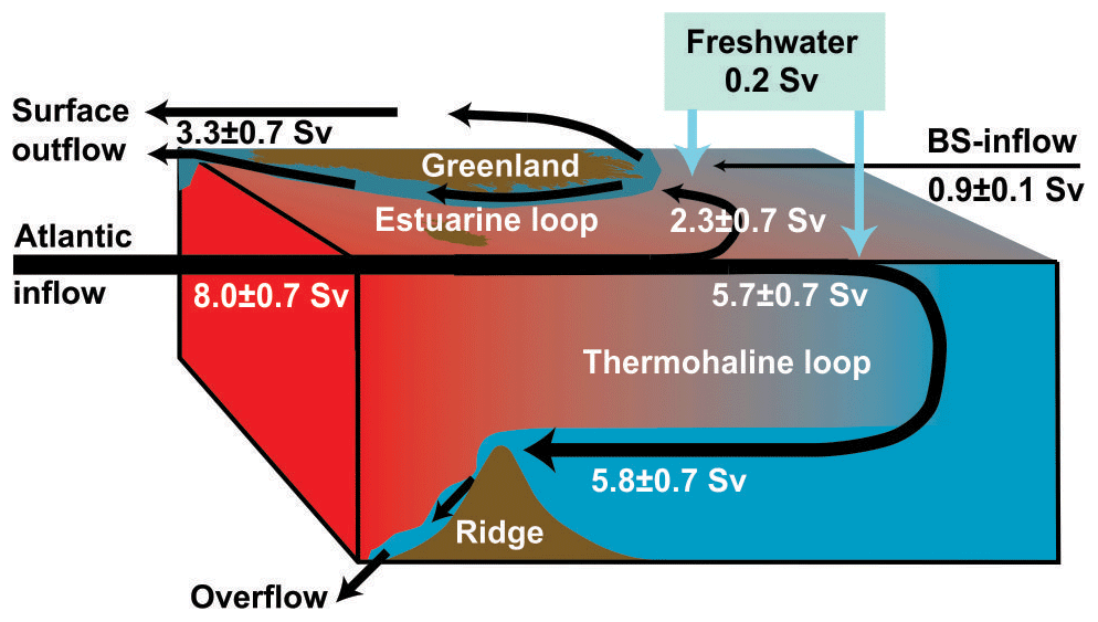
Figure 11Overall budget for the AM exchanges where the circulation within the AM is simplified into two loops: a thermohaline loop converting Atlantic inflow and freshwater into overflow, and an estuarine loop converting all three types of AM import into surface outflow.
The non-contiguity of the combined observational system may perhaps also affect the seasonal variation in the net import (Fig. 8), but probably less than it affects the average balance. From this and the discussion in Sect. 4.2, we would therefore expect the AM export to have a seasonal amplitude close to 1 Sv and be strongest (most negative) around October. From our knowledge about the other export branches (Fig. 7b), most of this seasonality would have to come from the DS-outflow, which is consistent with the available knowledge (Jónsson, 1999; de Steur et al., 2017), but will have to await future observational efforts for confirmation. Meanwhile our time series will be combined with results from numerical models, reanalyses (Bringedal et al., 2018), and observations using other methods (Rossby et al., 2018).
For the purpose of this study, it might have been advantageous if the monitoring in the Greenland–Scotland region had used the same sections for import and export branches. The main motivation for monitoring these flows is, however, to observe their effects on conditions in the AM and on the AMOC. That purpose may be better served by locating some of the monitoring sections somewhat downstream from the intensive mixing areas over the Greenland–Scotland Ridge.
4.5 The AM as a double estuary
It is well known (e.g. Rudels, 2010) that the AM may be seen as a double estuary with both an estuarine and a thermohaline circulation. In Fig. 11, the Atlantic inflow is split into two parts by two circulatory loops that feed the overflow and the surface outflow, respectively. The water mass transformations associated with the formation of overflow water occur in the Nordic Seas and the shelf seas north of Eurasia (Hansen and Østerhus, 2000). The Atlantic inflow is cooled by the atmosphere and freshened by mixing with freshwater. The low-density Pacific water enters through the Bering Strait and most of it leaves through the Canadian Arctic Archipelago (Rudels et al., 2004) although Bering Strait waters are also found in the Fram Strait in some years (Falck, 2001). Most of this low-density water mass does therefore not pass through the overflow-formation areas and is not likely to contribute appreciably to overflow production (although it may affect water transformations outside the AM, e.g. in the Labrador Sea).
To a first approximation, overflow water may therefore be considered a mixture of Atlantic water and freshwater in a mixing ratio of 99:1, based on the typical salinities of Atlantic water (∼35.3; González-Pola et al., 2018) and overflow water (∼34.9; Jochumsen et al., 2012; Hansen and Østerhus, 2007). To produce 5.8 Sv of overflow water therefore requires Sv of freshwater, i.e. roughly one-third of the total Freshwater input, and Sv of Atlantic water (Fig. 11).
This budget implies that around 70 % of the total Atlantic inflow to the AM returns to the Atlantic through the thermohaline loop in the form of overflow. The remaining 30 % of the Atlantic inflow enters the estuarine loop where it joins the BS-inflow and the remainder of the Freshwater input. With the numbers in Fig. 11, Atlantic inflow supplies around 70 % of the total surface outflow and BS-inflow somewhat more than 25 %, but these numbers are of course sensitive to the uncertainties involved.
4.6 Long-term variations in the AM exchanges
The exchanges between the AM and the rest of the World Ocean, the AM exchanges, are an integral part of the AMOC. With a total volume transport close to 6 Sv (Fig. 11), the overflows contribute the densest third to the production of NADW. The overflow contribution to the NADW is furthermore augmented by the waters entrained downstream of the Greenland–Scotland Ridge (e.g. Dickson and Brown, 1994; Fogelqvist et al., 2003; Hansen et al., 2004) and probably exceeds the additional contribution from convection in the Labrador Sea substantially (Lozier et al., 2019).
With that in mind, the projected weakening of the AMOC (Collins et al., 2014) might well be expected to affect the AM exchanges, but a closer scrutiny of the different climate models demonstrates huge differences in the projections for that part of the AMOC that involves the AM (Sgubin et al., 2017). For most of the world, it may not be important which source for the AMOC weakens, but that is not the case for the regions affected by the poleward heat transport associated with the upper limb of the AMOC. Thus, conditions in the AM are critically dependent on the heat imported by the Atlantic inflows (Skagseth and Mork, 2012; Mork et al., 2014; Årthun et al., 2012, 2017; Onarheim et al., 2014; Utne et al., 2012). The effect of the oceanic heat transport on Arctic sea ice (Zhang, 2015), and vice versa (Bitz et al., 2007), is also speculated to feed back on mid-latitude weather systems, currently a research topic of high interest (e.g. http://www.blue-action.eu, last access: 1 April 2019).
It is therefore highly relevant to ask whether our data indicate any weakening over their observational periods, which exceed two decades for the longest observed branches. The brief answer to this question is no. On the contrary, the only significant trend found is the Pacific inflow, which showed an increasing (not weakening) trend (Table 2), while the Atlantic inflow as well as the two dominant overflow branches remained stable (Fig. 9).
A priori, this result may seem to be in conflict with reports of AMOC weakening 2004–2012 at 26∘ N (Smeed et al., 2014) especially since they found the weakening to be due to a slowing of the southward flow of “lower NADW below 3000 m” by 7 % per year. Later measurements indicate that the North Atlantic Ocean went into a state of reduced overturning during the period 2008–2012 with a 30 % reduction of lower NADW between the periods 2004–2008 and 2008–2017 (Smeed et al., 2018). Generally (e.g. Orsi et al., 2001), lower NADW has been considered to be fed from overflows and entrained waters. One might therefore expect to see this reported weakening reflected in our data.
Instead, the two main overflow branches in our data set indicate no significant weakening during this period (Fig. 9b and thick blue line in Fig. 10) and this result is strengthened by the behaviour of the total Atlantic inflow (thick red line in Fig. 10), since the overflow and the Atlantic inflow must be strongly coupled through the thermohaline loop according to Fig. 11. Our results indicate that any weakening of the AMOC during the last two decades cannot have been caused by reduced overflow volume transport.
For the estuarine loop, increases have been reported for the BS-inflow (Woodgate et al., 2018) as well as the Freshwater input (e.g. Haine et al., 2015). These increases are, however, small compared to the total surface outflow. Thus, the overall picture for the AM exchanges is one of stability. It should be emphasized that the observed stability of volume transports does not imply that water mass properties also have remained stable during the last two decades. Rather, temperature and salinity have varied considerably for both the Pacific and the Atlantic inflows, although overall trends have been small (Woodgate et al., 2018; González-Pola et al., 2018). More persistent changes have been observed for the densest overflow branch, the FB-overflow, which has warmed consistently since around 2002, although density has remained stable due to concurrent salinity increase (Hansen et al., 2016).
Our finding that the AM exchanges have been stable in terms of volume transport during a period when many other components of the global climate system have changed is reassuring, but the possibility of future change remains (Sgubin et al., 2017). Continued increase in freshwater supply to the AM may act to destabilize the exchanges and so may change in the oceanic salt transport into the AM. The coupling between the Atlantic inflow and the overflow (Fig. 11) may be seen as a feedback mechanism (Stommel, 1961), which makes the thermohaline loop sensitive to the salinity of the Atlantic inflow. In this connection, the dramatic freshening of the Atlantic inflows since ∼2010 (González-Pola et al., 2018) is worrisome. This emphasizes the need to maintain and ideally expand the monitoring system.
Although the time series for many of the exchange branches in our data set have large gaps and are based on a non-contiguous observational system, we find that they do present a consistent picture of the total AM exchanges. The most complete coverage is for the AM import, consisting of the combined oceanic inflows and the Freshwater input. On average, the AM import is found to total 9.1±0.7 Sv with a fairly consistent seasonal variation that has an amplitude close to 1 Sv and maximum import around October.
Our data give a good balance between average import and export with only 0.4 Sv more water being exported than imported on the average, which is well below the combined quoted uncertainties. The imbalance in the seasonal variations, indicated by our data, is probably caused by our lack of simultaneous coverage of all the export branches, especially our very limited data set for the surface outflow through the Denmark Strait.
We therefore argue that the five oceanic inflow branches and the two main overflow branches most likely do give a good representation of the long-term variations and none of them weakened. Thus, the AM exchanges as a whole are not likely to have weakened during the two decades from the mid-1990s to the mid-2010s. Certainly, the combined transport of the two main overflow branches did not weaken and they account for almost 90 % of the total overflow.
Around 70 % of the Atlantic inflow is converted into overflow and the observed stability of the total Atlantic inflow further indicates that the thermohaline loop of the AM remained stable during our observational period. Although the overflow is a key component of the AMOC, any weakening of the AMOC during this period cannot have been caused by weakened overflow or weakened overturning in the AM.
Our finding that the exchanges have not weakened during the last two decades of global change is reassuring, but it is no guarantee of future stability. Keeping in mind the importance of these exchanges for conditions in the AM and more globally, we therefore strongly recommend that all possible efforts are made to maintain the established monitoring systems and preferably expand them. These systems are demanding in labour and continued funding and short-term scientific discoveries are not always guaranteed, but they are the safest way to stay alert against possible future changes since it is not yet clear where and how a disruption of the AM-exchange systems will first be manifested or which indices may serve as early warning indicators.
The observational data used in this study are available online at http://www.oceansites.org/tma/gsr.html (last access: 1 April 2019), http://www.bodc.ac.uk (last access: 1 April 2019), http://iop.apl.washington.edu/data.html (last access: 1 April 2019), and http://psc.apl.washington.edu/HLD/Bstrait/bstrait.html (last access: 1 April 2019).
The supplement related to this article is available online at: https://doi.org/10.5194/os-15-379-2019-supplement.
All authors provided data and contributed to the writing process lead by SØ, BH, and KMHL.
The authors declare that they have no conflict of interest.
This study was supported by European Framework Programmes under grant agreement no. GA212643 (THOR) and grant agreement no. 308299 (NACLIM), and from the European Union's Horizon 2020 research and innovation programme under grant agreement no. 727852 (Blue-Action). Bering Strait data and analysis were supported by NSF-Office of Polar Programs Arctic Observing Network grants PLR-1304052 & PLR-1758565. The Davis Strait program (CML and BC) was supported by the US National Science Foundation under grants OPP0230381, ARC0632231, and ARC1022472, with additional support from the Department of Fisheries and Oceans, Canada. We thank Wilken-Jon von Appen and an anonymous referee for very constructive comments.
This paper was edited by Mario Hoppema and reviewed by Wilken-Jon von Appen and one anonymous referee.
Aagaard, K. and Carmack, E. C.: The role of sea ice and other fresh water in the Arctic circulation, J. Geophys. Res., 94, 14485–14498, https://doi.org/10.1029/JC094iC10p14485, 1989.
Allen, J. T., Smeed, D. A., and Chadwick, A. L.: Eddies and mixing at the Iceland-Faroes Front, Deep-Sea Res. Pt. I, 41, 51–79, https://doi.org/10.1016/0967-0637(94)90026-4,1994.
Andersen, O. B. and Piccioni, G.: Recent Arctic Sea Level Variations from Satellites, Front. Mar. Sci., 3, 1–6, https://doi.org/10.3389/fmars.2016.00076, 2016.
Årthun, M., Eldevik, T., Smedsrud, L. H., Skagseth, Ø., and Ingvaldsen, R. B.: Quantifying the Influence of Atlantic Heat on Barents Sea Ice Variability and Retreat, J. Climate, 25, 4736–4743, https://doi.org/10.1175/JCLI-D-11-00466.1, 2012.
Årthun, M., Eldevik, T., Viste, E., Drange, H., Furevik, T., Johnson, H. L., and Keenlyside, N. S.: Skillful prediction of northern climate provided by the ocean, Nat. Commun., 8, 15875, https://doi.org/10.1038/ncomms15875, 2017.
Bacon, S., Reverdin, G., Rigor, I. G., and Snaith, H. M.: A freshwater jet on the east Greenland shelf, J. Geophys. Res.-Oceans, 107, 3068, https://doi.org/10.1029/2001JC000935, 2002.
Beaird, N. L., Rhines, P. B., and Eriksen, C. C.: Overflow Waters at the Iceland–Faroe Ridge Observed in Multiyear Seaglider Surveys, J. Phys. Oceanogr., 43, 2334–2351, https://doi.org/10.1175/JPO-D-13-029.1, 2013.
Bergström, S. and Carlsson, B.: River runoff to the Baltic Sea: 1950–1990, Ambio, 23, 280–287, 1994.
Berx, B., Hansen, B., Østerhus, S., Larsen, K. M., Sherwin, T., and Jochumsen, K.: Combining in situ measurements and altimetry to estimate volume, heat and salt transport variability through the Farœ–Shetland Channel, Ocean Sci., 9, 639–654, https://doi.org/10.5194/os-9-639-2013, 2013.
Beszczynska-Möller, A., Woodgate, R., Lee, C., Melling, H., and Karcher, M.: A Synthesis of Exchanges Through the Main Oceanic Gateways to the Arctic Ocean, Oceanography, 24, 82–99, https://doi.org/10.5670/oceanog.2011.59, 2011.
Bitz, C. M., Gent, P. R., Woodgate, R. A., Holland, M. M., and Lindsay, R.: The Influence of Sea Ice on Ocean Heat Uptake in Response to Increasing CO2, J. Climate, 20, 2437–2450, https://doi.org/10.1175/JCLI3756.1, 2007.
Borenäs, K. M. and Lundberg, P. A.: On the deep-water flow through the Faroe Bank Channel, J. Geophys. Res., 93, 1281–1292, https://doi.org/10.1029/JC093iC02p01281, 1988.
Bringedal, C., Eldevik, T., Skagseth, Ø., Spall, M. A., and Østerhus, S.: Structure and Forcing of Observed Exchanges across the Greenland–Scotland Ridge, J. Climate, 31, 9881–9901, https://doi.org/10.1175/JCLI-D-17-0889.1, 2018.
Chafik, L.: The response of the circulation in the Faroe-Shetland Channel to the North Atlantic Oscillation, Tellus A, 64, 18423, https://doi.org/10.3402/tellusa.v64i0.18423, 2012.
Childers, K. H., Flagg, C. N., and Rossby, T.: Direct velocity observations of volume flux between Iceland and the Shetland Islands, J. Geophys. Res.-Oceans, 119, 5934–5944, https://doi.org/10.1002/2014JC009946, 2014.
Collins, M., Knutti, R., Arblaster, J., Dufresne, J.-L., Fichefet, T., Friedlingstein, P., Gao, X., Gutowski, W. J., Johns, T., Krinner, G., Shongwe, M., Tebaldi, C., Weaver, A. J., and Wehner, M.: Long-term Climate Change: Projections, Commitments and Irreversibility, chap. 12, in: Climate Change 2013: The Physical Science Basis, Contribution of Working Group I to the Fifth Assessment Report of the Intergovernmental Panel on Climate Change, edited by: Stocker, T. F., Qun, D., Plattner, G.-K., M. Tignor, Allen, S. K., Doschung, J., Nauels, A., Xia, Y., Bex, V., and Midgley, P. M., Cambridge University Press, Cambridge, United Kingdom and New York, NY, USA, https://doi.org/10.1017/CBO9781107415324.024, 2014.
Cuny, J., Rhines, P. B., Niiler, P. P., and Bacon, S.: Labrador Sea Boundary Currents and the Fate of the Irminger Sea Water, J. Phys. Oceanogr., 32, 627–647, https://doi.org/10.1175/1520-0485(2002)032<0627:LSBCAT>2.0.CO;2, 2002.
Curry, B., Lee, C. M., Petrie, B., Moritz, R. E., and Kwok, R.: Multiyear Volume, Liquid Freshwater, and Sea Ice Transports through Davis Strait, 2004–10, J. Phys. Oceanogr., 44, 1244–1266, https://doi.org/10.1175/JPO-D-13-0177.1, 2014.
de Steur, L., Hansen, E., Gerdes, R., Karcher, M., Fahrbach, E., and Holfort, J.: Freshwater fluxes in the East Greenland Current: A decade of observations, Geophys. Res. Lett., 36, L23611, https://doi.org/10.1029/2009GL041278, 2009.
de Steur, L., Pickart, R. S., Macrander, A., Våge, K., Harden, B., Jónsson, S., Østerhus, S., and Valdimarsson, H.: Liquid freshwater transport estimates from the East Greenland Current based on continuous measurements north of Denmark Strait, J. Geophys. Res.-Oceans, 122, 93–109, https://doi.org/10.1002/2016JC012106, 2017.
Dickson, R. R. and Brown, J.: The production of North Atlantic Deep Water: Sources, rates, and pathways, J. Geophys. Res., 99, 12319–12341, https://doi.org/10.1029/94JC00530, 1994.
Dickson, R., Rudels, B., Dye, S., Karcher, M., Meincke, J., and Yashayaev, I.: Current estimates of freshwater flux through Arctic and subarctic seas, Prog. Oceanogr., 73, 210–230, https://doi.org/10.1016/j.pocean.2006.12.003, 2007.
Dooley, H. D. and Meincke, J.: Circulation and water masses in the Faroese Channels during overflow '73, Deut. Hydrogr. Z., 34, 41–55, https://doi.org/10.1007/BF02226585, 1981.
Ellett, D. J. and Roberts, D. G.: The overflow of Norwegian Sea Deep water across the Wyville-Thomson Ridge, Deep-Sea Res. Pt. I, 20, 819–835, https://doi.org/10.1016/0011-7471(73)90004-1, 1973.
Falck, E.: Contribution of waters of Atlantic and Pacific origin in the Northeast Water Polynya, Polar Res., 20, 193–200, https://doi.org/10.3402/polar.v20i2.6517, 2001.
Fischer, J., Karstensen, J., Zantopp, R., Visbeck, M., Biastoch, A., Behrens, E., Böning, C. W., Quadfasel, D., Jochumsen, K., Valdimarsson, H., Jónsson, S., Bacon, S., Holliday, N. P., Dye, S., Rhein, M., and Mertens, C.: Intra-seasonal variability of the DWBC in the western subpolar North Atlantic, Prog. Oceanogr., 132, 233–249, https://doi.org/10.1016/j.pocean.2014.04.002, 2015.
Fogelqvist, E., Blindheim, J., Tanhua, T., Østerhus, S., Buch, E., and Rey, F.: Greenland–Scotland overflow studied by hydro-chemical multivariate analysis, Deep-Sea Res. Pt. I, 50, 73–102, https://doi.org/10.1016/S0967-0637(02)00131-0, 2003.
Gebbie, G. and Huybers, P.: Total Matrix Intercomparison: A Method for Determining the Geometry of Water-Mass Pathways, J. Phys. Oceanogr., 40, 1710–1728, https://doi.org/10.1175/2010JPO4272.1, 2010.
González-Pola, C., Larsen, K. M. H., Fratantoni, P., Beszczynska-Möller, A., and Hughes, S. L. (Eds.): ICES Report on Ocean Climate 2016, ICES Cooperative Research Report No. 339, 110 pp., https://doi.org/10.17895/ices.pub.4069, 2018.
Gould, W. J., Loynes, J., and Backhaus, J.: Seasonality in slope current transports NW of Shetland, ICES CM1985/C7, 1985.
Haine, T. W. N., Curry, B., Gerdes, R., Hansen, E., Karcher, M., Lee, C., Rudels, B., Spreen, G., de Steur, L., Stewart, K. D., and Woodgate, R.: Arctic freshwater export: Status, mechanisms, and prospects, Global Planet. Change, 125, 13–35, https://doi.org/10.1016/j.gloplacha.2014.11.013, 2015.
Hansen, B. and Meincke, J.: Eddies and meanders in the Iceland-Faroe Ridge area, Deep-Sea Res., 26, 1067–1082, https://doi.org/10.1016/0198-0149(79)90048-7, 1979.
Hansen, B. and Østerhus, S.: North Atlantic–Nordic Seas exchanges, Prog. Oceanogr., 45, 109–208, https://doi.org/10.1016/S0079-6611(99)00052-X, 2000.
Hansen, B. and Østerhus, S.: Faroe Bank Channel overflow 1995–2005, Prog. Oceanogr., 75, 817–856, https://doi.org/10.1016/j.pocean.2007.09.004, 2007.
Hansen, B., Østerhus, S., Hátún, H., Kristiansen, R., and Larsen, K. M. H.: The Iceland–Faroe inflow of Atlantic water to the Nordic Seas, Prog. Oceanogr., 59, 443–474, https://doi.org/10.1016/j.pocean.2003.10.003, 2003.
Hansen, B., Østerhus, S., Quadfasel, D., and Turrell, W.: Already the day after tomorrow?, Science, 305, 953–954, https://doi.org/10.1126/science.1100085, 2004.
Hansen, B., Østerhus, S., Turrell, W. R., Jónsson, S., Valdimarsson, H., Hátún, H., and Olsen, S. M.: The Inflow of Atlantic Water, Heat, and Salt to the Nordic Seas Across the Greenland–Scotland Ridge, in: Arctic–Subarctic Ocean Fluxes, edited by: Dickson, R. R., Meincke, J., and Rhines, P., Springer, Dordrecht, 15–43, https://doi.org/10.1007/978-1-4020-6774-7_2, 2008.
Hansen, B., Hátn, H., Kristiansen, R., Olsen, S. M., and Østerhus, S.: Stability and forcing of the Iceland-Faroe inflow of water, heat, and salt to the Arctic, Ocean Sci., 6, 1013–1026, https://doi.org/10.5194/os-6-1013-2010, 2010.
Hansen, B., Larsen, K. M. H., Hátún, H., Kristiansen, R., Mortensen, E., and Østerhus, S.: Transport of volume, heat, and salt towards the Arctic in the Faroe Current 1993–2013, Ocean Sci., 11, 743–757, https://doi.org/10.5194/os-11-743-2015, 2015.
Hansen, B., Húsgarð Larsen, K. M., Hátún, H., and Østerhus, S.: A stable Faroe Bank Channel overflow 1995–2015, Ocean Sci., 12, 1205–1220, https://doi.org/10.5194/os-12-1205-2016, 2016.
Hansen, B., Poulsen, T., Húsgarð Larsen, K. M., Hátún, H., Østerhus, S., Darelius, E., Berx, B., Quadfasel, D., and Jochumsen, K.: Atlantic water flow through the Faroese Channels, Ocean Sci., 13, 873–888, https://doi.org/10.5194/os-13-873-2017, 2017.
Hansen, B., Larsen, K. M. H., Olsen, S. M., Quadfasel, D., Jochumsen, K., and Østerhus, S.: Overflow of cold water across the Iceland–Farœ Ridge through the Western Valley, Ocean Sci., 14, 871–885, https://doi.org/10.5194/os-14-871-2018, 2018.
Harden, B. E., Pickart, R. S., Valdimarsson, H., Våge, K., de Steur, L., Richards, C., Bahr, F., Torres, D., Børve, E., Jónsson, S., Macrander, A., Østerhus, S., Håvik, L., and Hattermann, T.: Upstream sources of the Denmark Strait Overflow: Observations from a high-resolution mooring array, Deep-Sea Res. Pt. I, 112, 94–112, https://doi.org/10.1016/j.dsr.2016.02.007, 2016.
Hátún, H.: The Faroe Current, PhD thesis, University of Bergen, Norway, 2004.
Helland-Hansen, B. and Nansen, F.: The Norwegian Sea, its physical oceanography, Based on the Norwegian researches 1900–1904, Report on Norwegian fishery and marine-investigations, Det Mallingske Bogtrykkeri, Kristiania, Norway, Vol. 11, No. 2, 390 p., 1909.
Hermann, F.: Hydrographic observations in the Faroe Bank Channel and over the Faroe–Iceland Ridge June 1959, J. Cons. Int. pour Explor. Mer., 118, 5 pp., 1959.
Hermann, F.: The T–S diagram analysis of the water masses over the Iceland–Faroe Ridge and in the Faroe Bank Channel (Overflow '60), Rapp. PV Reun. Cons. Int. pour Explor. Mer., 157, 139–149, 1967.
Hill, A. E., Brown, J., Fernand, L., Holt, J., Horsburgh, K. J., Proctor, R., Raine, R., and Turrell, W. R.: Thermohaline circulation of shallow tidal seas, Geophys. Res. Lett., 35, L11605, https://doi.org/10.1029/2008GL033459, 2008.
IPCC: Climate Change 2013 – The Physical Science Basis: Working Group I Contribution to the Fifth Assessment Report of the Intergovernmental Panel on Climate Change, edited by: Stocker, T. F., Qin, D., Plattner, G. K., Tignor, M., Allen, S. K., Boschung, J., Nauels, A., Xia, Y., Bex, V., and Midgley, P. M., Cambridge University Press; Cambridge, UK and New York, NY, USA, 1535 pp., https://doi.org/10.1017/CBO9781107415324.005, 2013.
Jochumsen, K., Quadfasel, D., Valdimarsson, H., and Jónsson, S.: Variability of the Denmark Strait overflow: Moored time series from 1996–2011, J. Geophys. Res.-Oceans, 117, C12003, https://doi.org/10.1029/2012JC008244, 2012.
Jochumsen, K., Moritz, M., Nunes, N., Quadfasel, D., Larsen, K. M. H., Hansen, B., Valdimarsson, H., and Jónsson, S.: Revised transport estimates of the Denmark Strait overflow, J. Geophys. Res.-Oceans, 122, 3434–3450, https://doi.org/10.1002/2017JC012803, 2017.
Johnson, C., Sherwin, T., Cunningham, S., Dumont, E., Houpert, L., and Holliday, N. P.: Transports and pathways of overflow water in the Rockall Trough, Deep-Sea Res. Pt. I, 122, 48–59, https://doi.org/10.1016/j.dsr.2017.02.004, 2017.
Jónsson, S.: The Circulation in the northern part of the Denmark Strait, ICES CM/1999/L, 1999.
Jónsson, S. and Valdimarsson, H.: The flow of Atlantic water to the North Icelandic Shelf and its relation to the drift of cod larvae, ICES J. Mar. Sci., 62, 1350–1359, https://doi.org/10.1016/j.icesjms.2005.05.003, 2005.
Jónsson, S. and Valdimarsson, H.: Water mass transport variability to the North Icelandic shelf, 1994–2010, ICES J. Mar. Sci., 69, 809–815, https://doi.org/10.1093/icesjms/fss024, 2012.
Knudsen, M.: Den Danske Ingolf-expedition, Bianco Lunos Kgl. Hof-Bogtrykkeri (F. Dreyer), København, 1898.
Käse, R. H., Girton, J. B., and Sanford, T. B.: Structure and variability of the Denmark Strait Overflow: Model and observations, J. Geophys. Res.-Oceans, 108, 3181, https://doi.org/10.1029/2002JC001548, 2003.
Larsen, K. M. H., Hansen, B., and Svendsen, H.: Faroe Shelf Water, Cont. Shelf Res., 28, 1754–1768, https://doi.org/10.1016/j.csr.2008.04.006, 2008.
Lozier, M. S., Li, F., Bacon, S., Bahr, F., Bower, A. S., Cunningham, S. A., de Jong, M. F., de Steur, L., deYoung, B., Fischer, J., Gary, S. F., Greenan, B. J. W., Holliday, N. P., Houk, A., Houpert, L., Inall, M. E., Johns, W. E., Johnson, H. L., Johnson, C., Karstensen, J., Koman, G., Le Bras, I. A., Lin, X., Mackay, N., Marshall, D. P., Mercier, H., Oltmanns, M., Pickart, R. S., Ramsey, A. L., Rayner, D., Straneo, F., Thierry, V., Torres, D. J., Williams, R. G., Wilson, C., Yang, J., Yashayaev, I., and Zhao, J.: A sea change in our view of overturning in the subpolar North Atlantic, Science, 363, 516–521, https://doi.org/10.1126/science.aau6592, 2019.
Macrander, A., Send, U., Valdimarsson, H., Jónsson, S., and Käse, R. H.: Interannual changes in the overflow from the Nordic Seas into the Atlantic Ocean through Denmark Strait, Geophys. Res. Lett., 32, L06606, https://doi.org/10.1029/2004GL021463, 2005.
Mastropole, D., Pickart, R. S., Valdimarsson, H., Våge, K., Jochumsen, K., and Girton, J.: On the hydrography of Denmark Strait, J. Geophys. Res.-Oceans, 122, 306–321, https://doi.org/10.1002/2016JC012007, 2017.
Mauritzen, C.: Production of dense overflow waters feeding the North Atlantic across the Greenland-Scotland Ridge. Part 1: Evidence for a revised circulation scheme, Deep-Sea Res. Pt. I, 43, 769–806, https://doi.org/10.1016/0967-0637(96)00037-4, 1996.
Meincke, J.: On the distribution of low salinity intermediate waters around the Faroes, Deut. Hydrogr. Z., 31, 50–64, https://doi.org/10.1007/BF02226000, 1978.
Meincke, J.: The Modern Current Regime Across the Greenland-Scotland Ridge, in: Structure and Development of the Greenland-Scotland Ridge, edited by: Bott, M. H. P., Saxov, S., Talwani, M., and Thiede, J., NATO Conference Series (IV Marine Science), 8, Springer, Boston, MA, 637–650, 1983.
Melling, H., Agnew, T. A., Falkner, K. K., Greenberg, D. A., Lee, C. M., Münchow, A., Petrie, B., Prinsenberg, S. J., Samelson, R. M., and Woodgate, R. A.: Fresh-Water Fluxes via Pacific and Arctic Outflows Across the Canadian Polar Shelf, in: Arctic–Subarctic Ocean Fluxes, edited by: Dickson, R. R., Meincke, J., and Rhines, P., Springer, Dordrecht, 193–247, https://doi.org/10.1007/978-1-4020-6774-7_10, 2008.
Morison, J., Wahr, J., Kwok, R., and Peralta-Ferriz, C.: Recent trends in Arctic Ocean mass distribution revealed by GRACE, Geophys. Res. Lett., 34, L07602, https://doi.org/10.1029/2006GL029016, 2007.
Mork, K. A. and Skagseth, Ø.: Annual sea surface height variability in the Nordic seas, in: The Nordic Seas: An Integrated Perspective Oceanography, Climatology, Biogeochemistry, and Modeling, edited by: Drange, H., Dokken, T., Furevik, T., Gerdes, R., and Berger, W., AGU Geophysical Monograph, 51–64, https://doi.org/10.1029/158GM05, 2005.
Mork, K. A., Skagseth, Ø., Ivshin, V., Ozhigin, V., Hughes, S. L., and Valdimarsson, H.: Advective and atmospheric forced changes in heat and fresh water content in the Norwegian Sea, 1951–2010, Geophys. Res. Lett., 41, 6221–6228, https://doi.org/10.1002/2014GL061038, 2014.
Myers, P. G., Kulan, N., and Ribergaard, M. H.: Irminger Water variability in the West Greenland Current, Geophys. Res. Lett., 34, L17601, https://doi.org/10.1029/2007GL030419, 2007.
Olsen, S. M., Hansen, B., Østerhus, S., Quadfasel, D., and Valdimarsson, H.: Biased thermohaline exchanges with the Arctic across the Iceland–Farœ Ridge in ocean climate models, Ocean Sci., 12, 545–560, https://doi.org/10.5194/os-12-545-2016, 2016.
Onarheim, I. H., Smedsrud, L. H., Ingvaldsen, R. B., and Nilsen, F.: Loss of sea ice during winter north of Svalbard, Tellus A, 66, 23933, https://doi.org/10.3402/tellusa.v66.23933, 2014.
Orsi, A. H., Jacobs, S. S., Gordon, A. L., and Visbeck, M.: Cooling and ventilating the Abyssal Ocean, Geophys. Res. Lett., 28, 2923–2926, https://doi.org/10.1029/2001GL012830, 2001.
Østerhus, S., Turrell, W. R., Hansen, B., Lundberg, P., and Buch, E.: Observed transport estimates between the North Atlantic and the Arctic Mediterranean in the Iceland–Scotland region, Polar Res., 20, 169–175, https://doi.org/10.3402/polar.v20i2.6514, 2001.
Østerhus, S., Sherwin, T., Quadfasel, D., and Hansen, B.: The Overflow Transport East of Iceland, in: Arctic–Subarctic Ocean Fluxes, edited by: Dickson, R. R., Meincke, J., and Rhines, P., Springer, Dordrecht, 427–441, https://doi.org/10.1007/978-1-4020-6774-7_19, 2008.
Peralta-Ferriz, C. and Morison, J.: Understanding the annual cycle of the Arctic Ocean bottom pressure, Geophys. Res. Lett., 37, L10603, https://doi.org/10.1029/2010GL042827, 2010.
Perkins, H., Hopkins, T. S., Malmberg, S. A., Poulain, P. M., and Warn-Varnas, A.: Oceanographic conditions east of Iceland, J. Geophys. Res.-Oceans, 103, 21531–21542, https://doi.org/10.1029/98JC00890, 1998.
Prandle, D.: Year-Long measurements of flow through the Dover Strait by H.F. Radar and acoustic Doppler current profiler (ADCP), Oceanol. Acta, 16, 457–468, 1993.
Radach, G. and Pätsch, J.: Variability of continental riverine freshwater and nutrient inputs into the North Sea for the years 1977–2000 and its consequences for the assessment of eutrophication, Estuar. Coast., 30, 66–81, https://doi.org/10.1007/BF02782968, 2007.
Read, J. F. and Pollard, R. T.: Water Masses in the Region of the Iceland–Færoes Front, J. Phys. Oceanogr., 22, 1365–1378, https://doi.org/10.1175/1520-0485(1992)022<1365:WMITRO>2.0.CO;2, 1992.
Roach, A. T., Aagaard, K., Pease, C. H., Salo, S. A., Weingartner, T., Pavlov, V., and Kulakov, M.: Direct measurements of transport and water properties through the Bering Strait, J. Geophys. Res., 100, 18443–18457, https://doi.org/10.1029/95JC01673, 1995.
Ross, C. K.: Temperature-salinity characteristics of the “overflow” water in Denmark Strait during “OVERFLOW '73”, Rapp. P.-v. Réun. Cons. int. Explor. Mer., 185, 111–119, 1984.
Rossby, T. and Flagg, C. N.: Direct measurement of volume flux in the Faroe-Shetland Channel and over the Iceland-Faroe Ridge, Geophys. Res. Lett., 39, L07602, https://doi.org/10.1029/2012GL051269, 2012.
Rossby, T., Prater, M. D., and Søiland, H.: Pathways of inflow and dispersion of warm waters in the Nordic seas, J. Geophys. Res., 114, C04011, https://doi.org/10.1029/2008JC005073, 2009.
Rossby, T., Flagg, C., Chafik, L., Harden, B., and Søiland, H.: A Direct Estimate of Volume, Heat, and Freshwater Exchange Across the Greenland-Iceland-Faroe-Scotland Ridge, J. Geophys. Res.-Oceans, 123, 7139–7153, https://doi.org/10.1029/2018JC014250, 2018.
Rudels, B.: Constraints on exchanges in the Arctic Mediterranean – do they exist and can they be of use?, Tellus A, 62, 109–122, https://doi.org/10.1111/j.1600-0870.2009.00425.x, 2010.
Rudels, B., Friedrich, H. J., and Quadfasel, D.: The Arctic Circumpolar Boundary Current, Deep-Sea Res. Pt. II, 46, 1023–1062, https://doi.org/10.1016/S0967-0645(99)00015-6, 1999.
Rudels, B., Jones, E. P., Schauer, U., and Eriksson, P.: Atlantic sources of the Arctic Ocean surface and halocline waters, Polar Res., 23, 181–208, https://doi.org/10.3402/polar.v23i2.6278, 2004.
Sabine, C. L., Feely, R. A., Gruber, N., Key, R. M., Lee, K., Bullister, J. L., Wanninkhof, R., Wong, C. S., Wallace, D. W., Tilbrook, B., Millero, F. J., Peng, T. H., Kozyr, A., Ono, T., and Rios, A. F.: The oceanic sink for anthropogenic CO2, Science, 305, 367–371, https://doi.org/10.1126/science.1097403, 2004.
Sætre, R.: Report on the Norwegian Investigations in the Faeroe Channel 1964–65, NATO Subcommittee on Oceanographic Research technical report, 27 pp., 1967.
Saunders, P., M.: The dense northern overflows, chap. 5.6, Ocean Circulation and Climate, edited by: Siedler, G., Church, J., and Gould, J., Int. Geophys., Academic Press, London, UK, 401–417, 2001.
Serreze, M. C., Barrett, A. P., Slater, A. G., Woodgate, R. A., Aagaard, K., Lammers, R. B., Steele, M., Moritz, R., Meredith, M., and Lee, C. M.: The large-scale freshwater cycle of the Arctic, J. Geophys. Res., 111, C11010, https://doi.org/10.1029/2005JC003424, 2006.
Sgubin, G., Swingedouw, D., Drijfhout, S., Mary, Y., and Bennabi, A.: Abrupt cooling over the North Atlantic in modern climate models, Nat. Commun., 8, 14375, https://doi.org/10.1038/ncomms14375, 2017.
Sherwin, T. J., Turrell, W. R., Jeans, D. R. G., and Dye, S.: Eddies and a mesoscale deflection of the slope current in the Faroe–Shetland Channel, Deep-Sea Res. Pt. I, 46, 415–438, https://doi.org/10.1016/S0967-0637(98)00077-6, 1999.
Sherwin, T. J., Williams, M. O., Turrell, W. R., Hughes, S. L., and Miller, P. I.: A description and analysis of mesoscale variability in the Färoe-Shetland Channel, J. Geophys. Res., 111, C03003, https://doi.org/10.1029/2005JC002867, 2006.
Sherwin, T. J., Griffiths, C. R., Inall, M. E., and Turrell, W. R.: Quantifying the overflow across the Wyville Thomson Ridge into the Rockall Trough, Deep-Sea Res. Pt. I, 55, 396–404, https://doi.org/10.1016/j.dsr.2007.12.006, 2008.
Skagseth, Ø. and Mork, K. A.: Heat content in the Norwegian Sea, 1995–2010, ICES J. Mar. Sci., 69, 826–832, https://doi.org/10.1093/icesjms/fss026, 2012.
Smeed, D. A., McCarthy, G. D., Cunningham, S. A., Frajka-Williams, E., Rayner, D., Johns, W. E., Meinen, C. S., Baringer, M. O., Moat, B. I., Duchez, A., and Bryden, H. L.: Observed decline of the Atlantic meridional overturning circulation 2004–2012, Ocean Sci., 10, 29–38, https://doi.org/10.5194/os-10-29-2014, 2014.
Smeed, D. A., Josey, S. A., Beaulieu, C., Johns, W. E., Moat, B. I., Frajka-Williams, E., Rayner, D., Meinen, C. S., Baringer, M. O., Bryden, H. L., and McCarthy, G. D.: The North Atlantic Ocean Is in a State of Reduced Overturning, Geophys. Res. Lett., 45, 1527–1533, https://doi.org/10.1002/2017GL076350, 2018.
Stefánsson, U.: North Icelandic waters, Rit Fiskideildar, 3, 269 pp., 1962.
Stommel, H.: Thermohaline Convection with Two Stable Regimes of Flow, Tellus, 13, 224–230, https://doi.org/10.3402/tellusa.v13i2.9491, 1961.
Straneo, F. and Saucier, F. J.: The Arctic–Subarctic Exchange Through Hudson Strait, in: Arctic–Subarctic Ocean Fluxes, edited by: Dickson, R. R., Meincke, J., and Rhines, P., Springer, Dordrecht, 249–261, https://doi.org/10.1007/978-1-4020-6774-7_11, 2008.
Sutherland, D. A. and Pickart, R. S.: The East Greenland Coastal Current: Structure, variability, and forcing, Prog. Oceanogr., 78, 58–77, https://doi.org/10.1016/j.pocean.2007.09.006, 2008.
Tait, J. B.: Hydrography of the Faroe–Shetland Channel 1927–1952, Scottish Home Department Marine Research, 2, 309 pp., 1957.
Tait, J. B.: The Iceland–Faroe Ridge international (ICES) “Overflow” expedition, May–June 1960, 71 pp., 1967.
Tang, C. C. L., Ross, C. K., Yao, T., Petrie, B., DeTracey, B. M., and Dunlap, E.: The circulation, water masses and sea-ice of Baffin Bay, Prog. Oceanogr., 63, 183–228, https://doi.org/10.1016/j.pocean.2004.09.005, 2004.
Turrell, W.: A Century of Hydrographic Observations, Ocean Challenge, 6, 58–63, 1995.
Turrell, W. R., Henderson, E. W., and Slesser, G.: Residual transport within the Fair Isle Current observed during the Autumn Circulation Experiment (ACE), Cont. Shelf Res., 10, 521–543, https://doi.org/10.1016/0278-4343(90)90080-6, 1990.
Utne, K. R., Huse, G., Ottersen, G., Holst, J. C., Zabavnikov, V., Jacobsen, J. A., Óskarsson, G. J., and Nøttestad, L.: Horizontal distribution and overlap of planktivorous fish stocks in the Norwegian Sea during summers 1995–2006, Mar. Biol. Res., 8, 420–441, https://doi.org/10.1080/17451000.2011.640937, 2012.
Volkov, D. L. and Pujol, M. I.: Quality assessment of a satellite altimetry data product in the Nordic, Barents, and Kara seas, J. Geophys. Res.-Oceans, 117, C03025, https://doi.org/10.1029/2011JC007557, 2012.
Willebrand, J. and Meincke, J.: Statistical analysis of fluctuations in the Iceland-Scotland frontal zone, Deep-Sea Res., 27, 1047–1066, https://doi.org/10.1016/0198-0149(80)90064-3, 1980.
Woodgate, R., Stafford, K., and Prahl, F.: A Synthesis of Year-Round Interdisciplinary Mooring Measurements in the Bering Strait (1990–2014) and the RUSALCA Years (2004–2011), Oceanography, 28, 46–67, https://doi.org/10.5670/oceanog.2015.57, 2015.
Woodgate, R. A.: Increases in the Pacific inflow to the Arctic from 1990 to 2015, and insights into seasonal trends and driving mechanisms from year-round Bering Strait mooring data, Prog. Oceanogr., 160, 124–154, https://doi.org/10.1016/j.pocean.2017.12.007, 2018.
Woodgate, R. A., Fahrbach, E., and Rohardt, G.: Structure and transports of the East Greenland Current at 75∘ N from moored current meters, J. Geophys. Res.-Oceans, 104, 18059–18072, https://doi.org/10.1029/1999JC900146, 1999.
Worthington, L. V.: The Norwegian Sea as a mediterranean basin, Deep-Sea Res. Pt. I, 17, 77–84, https://doi.org/10.1016/0011-7471(70)90088-4, 1970.
Zhang, R.: Mechanisms for low-frequency variability of summer Arctic sea ice extent, P. Natl. Acad. Sci. USA, 112, 4570–4575, https://doi.org/10.1073/pnas.1422296112, 2015.
Strictly speaking, all of the AM is part of the Atlantic Ocean, but we will follow common practice and reserve the term “Atlantic” for those regions of the Atlantic Ocean that are outside the AM.