Air–sea gas exchange at wind speeds up to 85 m s⁻¹

Gas transfer velocities were measured in two high-speed wind-wave tanks (Kyoto University and the SUSTAIN facility, RSMAS, University of Miami) using fresh water, simulated seawater and seawater for wind speeds between 7 and 85 m s⁻¹. Using a mass balance technique, transfer velocities of a total of 12 trace gases were measured, with dimensionless solubilities ranging from 0.005 to 150 and Schmidt numbers between 149 and 1360. This choice of tracers enabled the separation of gas transfer across the free interface from gas transfer at closed bubble surfaces. The major effect found was a very steep increase of the gas transfer across the free water surface at wind speeds beyond 33 m s⁻¹. The increase is the same for fresh water, simulated seawater and seawater. Bubble-induced gas transfer played no significant role for all tracers in fresh water and for tracers with moderate solubility such as carbon dioxide and dimethyl sulfide (DMS) in seawater, while for low-solubility tracers bubble-induced gas transfer in seawater was found to be about 1.7 times larger than the transfer at the free water surface at the highest wind speed of 85 m s⁻¹. There are indications that the low contributions of bubbles are due to the low wave age/fetch of the wind-wave tank experiments, but further studies on the wave age dependency of gas exchange are required to resolve this issue.

1 Introduction

The transfer of trace gases across the air–sea interface has been an active field of research for almost 40 years (Jähne, 2019). The transfer is characterized by the gas transfer velocity, which depends on environmental forcing such as the wind speed, the amount and strength of wave breaking, the presence of surface active material, number and size of bubbles, and spray created by breaking waves (Wanninkhof et al., 2009; Jähne, 2019).

Measuring the gas transfer velocity under hurricane conditions in the field is extremely challenging. Using unmanned floats, McNeil and D'Asaro (2007) managed to estimate three gas transfer velocities at wind speeds higher than 25 m s⁻¹ during Hurricane Frances in 2004. Due to the difficulties of measuring in the field, wind-wave tanks capable of producing hurricane force winds are a viable and safe alternative, as they allow for a controlled study of the air–sea interaction mechanisms up to the highest wind speeds.

Until now, only two gas transfer studies have been performed in hurricane conditions in the Kyoto High-Speed Wind-Wave Tank with 1,4-difluorobenzene and hexafluorobenzene (Krall and Jähne, 2014) and with carbon dioxide (Iwano et al., 2013, 2014) but only in fresh water. Both studies found a strong increase in the gas transfer velocity at wind speeds higher than approximately 33 to 35 m s⁻¹. Gas transfer was found to increase with more than the third power of the wind speed. However, because of the few gases used, it remains unclear which process is the main cause of this steep increase. Possible candidates are (a) bubbles, which provide an additional surface for the gas transfer, (b) an increased water surface area due to the fragmentation of the water surface at highest wind speeds or (c) a strong increase in near-surface turbulence due to frequent surface renewal and breakup events, or a combination of all three effects. It is also not clear whether bubble-induced gas exchange differs between fresh water and seawater.

This paper reports the results of extensive gas exchange measurements in two different wind-wave tanks with up to 12 tracers covering a wide range of solubilities using fresh water, simulated seawater and seawater.

2 Air–sea interactions

2.1 Gas transfer

The flux density j of a trace gas across a free, smooth or wavy unbroken air–sea interface is governed by the difference in concentration of the gas in air and water (c_a and c_w) and the gas transfer velocity k_s across the water surface:

$$\begin{array}{}\text{(1)}& j=k_{\mathrm{s}}\mathrm{\Delta }c=k_{\mathrm{s}}(c_{\mathrm{w}}-\mathit{\alpha }{c}_{\mathrm{a}}).\end{array}$$

Because of the discontinuity at the air–water boundary, the solubility α (here, α is equal to the dimensionless Henry solubility H^cc; Sander, 2015) has to be taken into account. The gas transfer velocity k_s of a sparingly soluble tracer through a free, smooth or wavy, unbroken surface can be described by

$$\begin{array}{}\text{(2)}& k_{\mathrm{s}}={\displaystyle \frac{\mathrm{1}}{\mathit{\beta }}}{u}_{\ast ,\mathrm{w}}S{c}^{-n},\end{array}$$

(Jähne et al., 1989) with the water-side friction velocity $u_{\ast ,\mathrm{w}}$, a measure for momentum input into the water by the wind, the Schmidt number $Sc=\mathit{\nu }/D$ of a tracer, given by the ratio of the kinematic viscosity of water ν and the tracer's diffusion coefficient in water D. The dimensionless parameter β and the Schmidt number exponent n depend on the boundary conditions, with $n=\mathrm{2}/\mathrm{3}$ for a smooth water surface and $n=\mathrm{1}/\mathrm{2}$ for a rough and wavy surface.

From Eq. (2), it is apparent that the transfer velocities of two sparingly soluble gases (A and B) can be converted by Schmidt number scaling:

$$\begin{array}{}\text{(3)}& {\displaystyle \frac{k_{\mathrm{s},A}}{k_{\mathrm{s},B}}}={\left({\displaystyle \frac{S{c}_A}{S{c}_B}}\right)}^{-n}.\end{array}$$

Commonly, a reference Schmidt number of Sc=600 is chosen, which corresponds to carbon dioxide at 20 ^∘C in fresh water.

For gases that have a medium to high solubility, the transfer resistance in the air side has to be taken into account. As first shown by Liss and Slater (1974), the total transfer velocity k_t can then be expressed by

$$\begin{array}{}\text{(4)}& {\displaystyle \frac{\mathrm{1}}{k_{\mathrm{t}}}}=\mathit{\alpha }{\displaystyle \frac{\mathrm{1}}{k_{\mathrm{a}}}}+{\displaystyle \frac{\mathrm{1}}{k_{\mathrm{s}}}},\end{array}$$

with k_a being the air-side transfer velocity. For gases with a low solubility, the second term dominates and the first term in Eq. (4) can be neglected, such that for those gases k_t=k_s. Inverse transfer velocities can be seen as transfer resistances, such that Eq. (4) can be written as

$$\begin{array}{}\text{(5)}& R_{\mathrm{t}}=\mathit{\alpha }{R}_{\mathrm{a}}+R_{\mathrm{s}}.\end{array}$$

All transfer velocities used in this paper are related to a water-side observer; i.e., they describe how fast a gas is transferred into or out of the water. Air-side observed gas transfer velocities differ by a factor of α.

2.2 Bubble-mediated gas transfer

Bubbles contribute to the gas transfer in two ways. First, they provide an additional surface through which gases can pass. Second, during their generation, by rising through the water-side mass boundary layer of the water surface and by bursting at the water surface, they increase the near-surface turbulence. Monahan and Spillane (1984) already considered whitecaps as “low impedance vents”, which “shortcut” the water-side transfer resistance. These bubble effects which intensify near-surface turbulence increase the transfer velocity across the free surface and do not depend on tracer solubility.

The transfer through a closed bubble surface is different from transfer across the free water surface. First, bubbles have a limited lifetime, as they either burst at the water surface or, if they are small enough, completely dissolve. Second, bubbles have a limited volume to take up or release gas. Once a bubble is filled to the equilibrium concentration $c_{\mathrm{b}}^{\mathrm{eq}}$ given by Henry's law, $c_{\mathrm{b}}^{\mathrm{eq}}={\mathit{\alpha }}^{-\mathrm{1}}{c}_{\mathrm{w}}$, it is inactive for the remainder of its lifetime. For gases with higher solubilities and for small bubbles, this equilibrium is reached faster. And third, bubbles experience an overpressure due to hydrostatic pressure and surface tension. Therefore, small bubbles can completely dissolve and the equilibrium concentration shifts to slightly higher concentrations. Because the measurements reported here are taken far from equilibrium, dissolving bubbles are not important. The transfer velocities themselves are not affected. A detailed analysis of the timescales involved and how they depend on the bubble radius is given in Jähne et al. (1984).

Because bubbles form an additional exchange surface, the total water-side transfer velocity k_w can be split up into two parts (Merlivat and Memery, 1983; Godal., 2016):

$$\begin{array}{}\text{(6)}& k_{\mathrm{w}}=k_{\mathrm{s}}+k_{\mathrm{c}},\end{array}$$

with transfer through the free water surface k_s and through the closed surface of submerged bubbles k_c. It is important to note here that the bubble-induced gas transfer velocity k_c does not include the bubble formation process and the bursting of bubbles when they rise through the surface again. Concerning the gas transfer velocity, these effects cannot be distinguished from other processes generating turbulence close to the water surface, because they do not depend on tracer solubility but only on the Schmidt number. Therefore, bubble-induced gas exchange refers here only to the stages in the lifetime of a bubble with a closed surface and therefore a limited trapped air volume.

Figure 1 shows a schematic view of the resistances for bubble-mediated gas transfer $R_{\mathrm{c}}=k_{\mathrm{c}}^{-\mathrm{1}}$ in relation to the air- and water-sided resistances for transfer through the unbroken water surface.

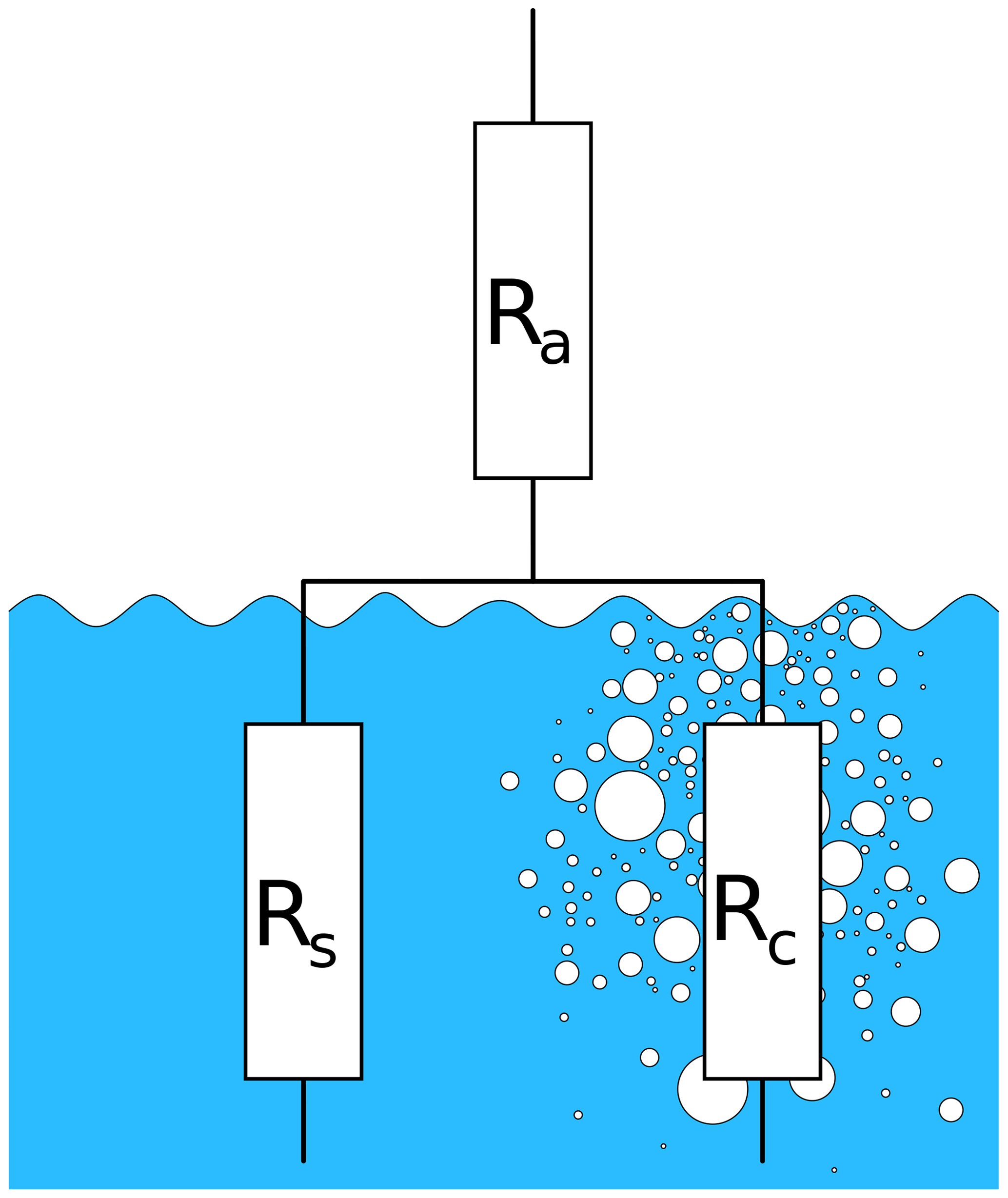
Figure 1 Transfer resistances: R_a: air-side transfer resistance, R_s: water-side resistance of the free water surface, R_c: transfer resistance of the closed bubble surfaces.

Many approaches have been made to quantify the bubble-mediated gas transfer k_c: gas transfer by single bubbles (Maiß, 1986; Patro et al., 2002), transfer in bubble clouds (Asher et al., 1996; Mischler, 2014) and breaking waves (Asher et al., 1995; Leifer and De Leeuw, 2002), as well as theoretical models based on bubble dynamics (Memery and Merlivat, 1985; Woolf and Thorpe, 1991). Bubble-mediated gas transfer also depends on bubble surface conditions. It has been shown that surface active material reduces the gas transfer of single bubbles (Maiß, 1986; Patro et al., 2002), while it also decreases the bubbles' rise velocity (Alves et al., 2005). During the lifetime of a bubble, these surface conditions can change, as bubbles accumulate surface active material while moving through the water.

Empirical or semi-empirical parameterizations (Godal., 2016; Woolf et al., 2007) are the state of the art of calculating the bubble-mediated gas transfer k_b on the open ocean. Most of these parameterizations link k_b to the tracer's solubility and Schmidt number (or diffusion coefficient) as well as the whitecap coverage of the water surface, which in turn depends on the sea state that is usually expressed as a function of the wind speed at 10 m height u₁₀ or the friction velocity $u_{\ast ,\mathrm{a}}$.

Physically based models (Woolf et al., 2007; Mischler, 2014) distinguish two limiting cases: one for very weakly soluble gases and one for more highly soluble ones. For very weakly soluble tracers, the bubbles act as a very big reservoir. In that case, the bubbles simply provide an additional surface for gas transfer that actively participates in gas transfer for the whole lifetime of a bubble. In this limit, the gas transfer is proportional to the integrated bubble surface area A_b,δr per radius interval δr normalized to the water surface area A_s and the Schmidt number with the bubble Schmidt number exponent n_b and does not depend on solubility:

$$\begin{array}{}\text{(7)}& \begin{array}{rl}{k}_{\mathrm{c},\mathrm{low}\mathit{\alpha }}& ={\displaystyle \frac{\int A_{\mathrm{b},\mathit{\delta }r}\left(r\right)k_{\mathrm{b},\mathrm{600}}\left(r\right)\mathrm{d}r}{A_{\mathrm{s}}}}{\left({\displaystyle \frac{\mathrm{600}}{Sc}}\right)}^{n_{\mathrm{b}}}\\ & =k_{\mathrm{c},\mathrm{600}}{\left({\displaystyle \frac{\mathrm{600}}{Sc}}\right)}^{n_{\mathrm{b}}}.\end{array}\end{array}$$

The transfer velocity k_c is the effective bubble-induced transfer velocity related to the free water surface, while k_b(r) is the real transfer velocity across the bubble surface of a given radius.

In the limit of high solubility, the bubbles constitute a very small reservoir for the trace gas, so that the higher-solubility tracers will reach concentration equilibrium $c_{\mathrm{b}}^{\mathrm{eq}}={\mathit{\alpha }}^{-\mathrm{1}}{c}_{\mathrm{w}}$ very fast. Then, the bubble-mediated gas transfer can only depend on the tracer's solubility and the total bubble volume flux Q_b,δr per radius interval δr:

$$\begin{array}{}\text{(8)}& k_{\mathrm{c},\mathrm{high}\mathit{\alpha }}={\displaystyle \frac{\mathrm{1}}{\mathit{\alpha }}}{\displaystyle \frac{\int Q_{\mathrm{b},\mathit{\delta }\mathrm{r}}\left(r\right)\mathrm{d}r}{A_{\mathrm{s}}}}={\displaystyle \frac{\mathrm{1}}{\mathit{\alpha }}}{\displaystyle \frac{Q_{\mathrm{b}}}{A_{\mathrm{s}}}}={\displaystyle \frac{\mathrm{1}}{\mathit{\alpha }}}{k}_{\mathrm{r}}.\end{array}$$

The velocity k_r has an intuitive meaning. It is the effective velocity (volume flux per water surface area) averaged over all bubble sizes, with which the air volume is being submerged by breaking waves and rises towards the surface again. Deike et al. (2017) call this quantity the air entrainment velocity V_a.

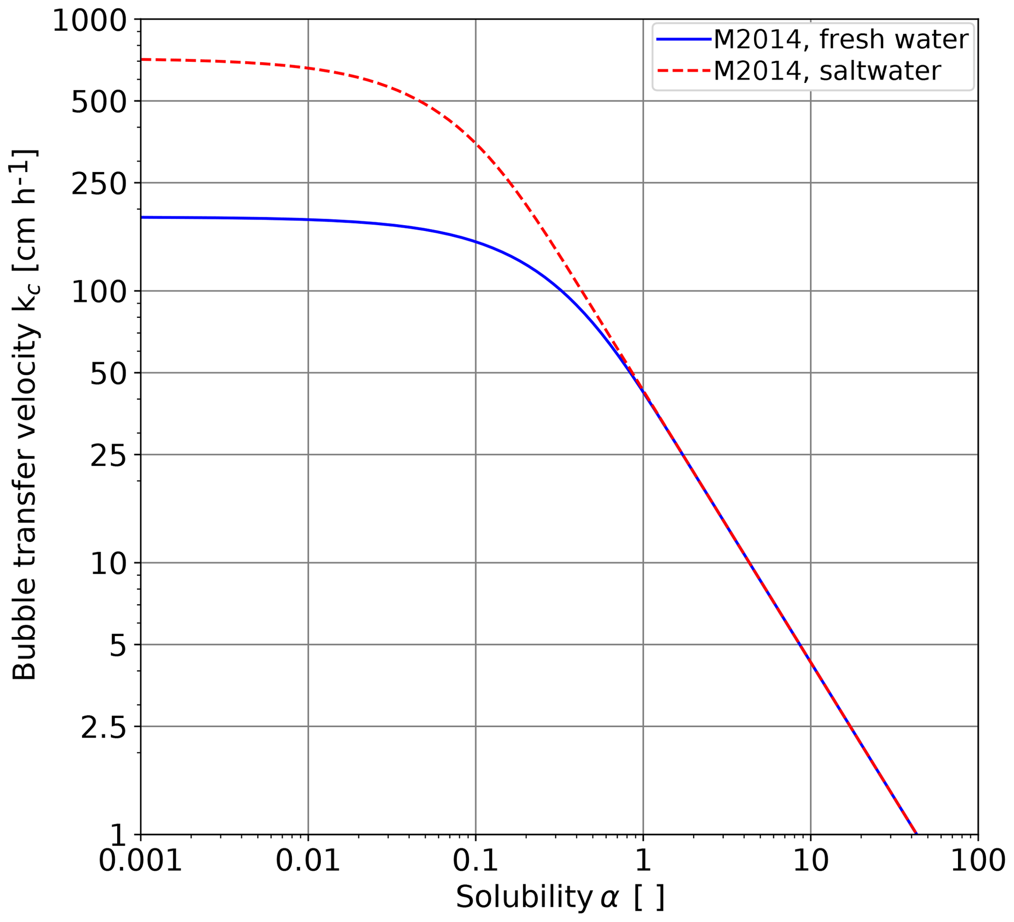
Figure 2 Dependency of bubble-mediated gas transfer velocities for the tracers covering a wide range of solubilities as measured in a bubble tank in which breaking waves were simulated by a water jet for fresh water and seawater (Mischler, 2014). The jet energy was 3.3 W and the bubble volume flux kept constant at about 750 mL min⁻¹, corresponding to k_r=43 cm h⁻¹.

The transition solubility, at which the constant bubble-mediated transfer velocity for low solubility k_c,low α changes into the transfer velocity decreasing with increasing solubility can be computed by setting both values equal:

$$\begin{array}{}\text{(9)}& {\mathit{\alpha }}_{\mathrm{t}}={\displaystyle \frac{k_{\mathrm{r}}}{k_{\mathrm{c},\mathrm{600}}}}{\left({\displaystyle \frac{Sc}{\mathrm{600}}}\right)}^{n_{\mathrm{b}}}.\end{array}$$

Based on detailed measurements in a bubble-tank with multiple volatile tracers, Mischler (2014) showed that the transition between the two regimes can be well described by a simple exponential term (Fig. 2). The transfer velocity for bubble-mediated gas exchange results in

$$\begin{array}{}\text{(10)}& k_{\mathrm{c}}={\displaystyle \frac{k_{\mathrm{r}}}{\mathit{\alpha }}}\left[\mathrm{1}-\exp \left(-{\displaystyle \frac{\mathit{\alpha }}{{\mathit{\alpha }}_{\mathrm{t}}}}\right)\right]=\left\{\begin{array}{ll}{k}_{\mathrm{c},\mathrm{600}}{\left({\displaystyle \frac{\mathrm{600}}{Sc}}\right)}^{n_{\mathrm{b}}}& \mathit{\alpha }\ll {\mathit{\alpha }}_{\mathrm{t}}\\ k_{\mathrm{r}}/\mathit{\alpha }& \mathit{\alpha }\gg {\mathit{\alpha }}_{\mathrm{t}}.\end{array}\right.\end{array}$$

For fresh water, Mischler (2014, Table 9.7) found, under the conditions shown in Fig. 2, a transition solubility α_t=0.23 for fresh water and 0.06 for seawater.

In summary, the total gas transfer velocity k_tot for water-side controlled tracers including bubble-mediated gas transfer can be parameterized as

$$\begin{array}{}\text{(11)}& \begin{array}{lll}{k}_{\mathrm{tot}}& =& k_{\mathrm{s}}+k_{\mathrm{c}}=k_{\mathrm{s},\mathrm{600}}{\left({\displaystyle \frac{\mathrm{600}}{Sc}}\right)}^{\mathrm{0.5}}\\ & +& {\displaystyle \frac{k_{\mathrm{r}}}{\mathit{\alpha }}}\left[\mathrm{1}-\exp \left(-{\displaystyle \frac{\mathit{\alpha }{k}_{\mathrm{c},\mathrm{600}}}{k_{\mathrm{r}}}}{\left({\displaystyle \frac{\mathrm{600}}{Sc}}\right)}^{\mathrm{0.5}}\right)\right],\end{array}\end{array}$$

with the three parameters k_s,600, k_c,600 and k_r. Because the measurements were performed with clean water, the Schmidt number exponents for both the transfer across the free water surface and the bubbles' surfaces are set to 1∕2. In the limits of low and high solubility, the model equation (Eq. 11) simplifies to

$$\begin{array}{}\text{(12)}& k_{\mathrm{tot}}=\left\{\begin{array}{ll}\left(k_{\mathrm{s},\mathrm{600}}+k_{\mathrm{c},\mathrm{600}}\right){\left({\displaystyle \frac{\mathrm{600}}{Sc}}\right)}^{\mathrm{0.5}}& \mathit{\alpha }\ll {\mathit{\alpha }}_{\mathrm{t}}\\ k_{\mathrm{s},\mathrm{600}}{\left({\displaystyle \frac{\mathrm{600}}{Sc}}\right)}^{\mathrm{0.5}}+k_{\mathrm{r}}/\mathit{\alpha }& \mathit{\alpha }\gg {\mathit{\alpha }}_{\mathrm{t}}.\end{array}\right.\end{array}$$

In the limit of low solubilities, the gas transfer velocity no longer depends on solubility, and simple Schmidt number scaling can be applied. The ratio of gas transfer across bubble surfaces and the free surface is then simply given by the ratio of k_c,600 to k_s,600.

Whereas, in Eq. (11), a parametric approach is given for the whole solubility range, Deike and Melville (2018, Eq. 12) provide only the high-solubility limit in a semi-empirical approach using field dimethyl sulfide (DMS) and CO₂ gas exchange measurements:

$$\begin{array}{}\text{(13)}& k_{\mathrm{tot}}=A_{\mathrm{NB}}{u}_{\ast ,\mathrm{a}}{\left({\displaystyle \frac{\mathrm{600}}{Sc}}\right)}^{\mathrm{0.5}}+{\displaystyle \frac{{\stackrel{\mathrm{̃}}{A}}_{\mathrm{b}}}{\mathit{\alpha }}}{u}_{\ast ,\mathrm{a}}^{\mathrm{2}}{c}_{\mathrm{p}},\end{array}$$

where in the second term $u_{\ast ,\mathrm{a}}^{\mathrm{5}/\mathrm{3}}(g{H}_{\mathrm{s}}{)}^{\mathrm{2}/\mathrm{3}}$ is replaced by the simpler term $u_{\ast ,\mathrm{a}}^{\mathrm{2}}{c}_{\mathrm{p}}$ using the Toba (1972) relation for fetch-limited waves. The term ${\stackrel{\mathrm{̃}}{A}}_{\mathrm{b}}{u}_{\ast ,\mathrm{a}}^{\mathrm{2}}{c}_{\mathrm{p}}$ is the air entrainment velocity V_a=k_r, which, according to Deike and Melville (2018), is increasing with the phase speed c_p of the peak wave or its significant weight height H_s, respectively. Surprisingly, Deike et al. (2017) found the air entrainment velocity decreasing with the wave age $c_{\mathrm{p}}/u_{\ast ,\mathrm{a}}$ by estimating the air entrainment velocity directly based on a model for a single breaking wave and the statistics of breaking waves as measured in the field.

2.3 Spray-mediated gas transfer

The processes mirroring bubbles in the water, which are spray droplets in the air, are less well studied, with the exception of the transfer of water vapor and heat (Mestayer and Lefauconnier, 1988; Andreas and Emanuel, 2001; Zheng et al., 2008; Jeong et al., 2012; Komori et al., 2018). Only recently, Andreas et al. (2017) evaluated the timescales governing spray-mediated gas transfer for gases other than water vapor in a similar fashion as Jähne et al. (1984) did for bubble-mediated transfer more than three decades earlier.

In contrast to bubbles, tracer solubility plays no role for spray droplets as long as the transfer process is controlled by water-sided processes. This is the case for all tracers used. Therefore, spray droplets just constitute an additional exchange surface. The question is only whether the lifetime for gas exchange is longer than the lifetime of the droplets. If this is the case, gas exchange occurs during their whole lifetime. In this upper limit, the gas transfer velocity k_d induced by spray droplet is given in analogy to Eq. (7) by

$$\begin{array}{}\text{(14)}& \begin{array}{rl}{k}_{\mathrm{d},\mathrm{upper}}& ={\displaystyle \frac{\int A_{\mathrm{d},\mathit{\delta }r}\left(r\right)k_{\mathrm{d},\mathrm{600}}\left(r\right)\mathrm{d}r}{A_{\mathrm{s}}}}{\left({\displaystyle \frac{\mathrm{600}}{Sc}}\right)}^{n_{\mathrm{d}}}\\ & =k_{\mathrm{d},\mathrm{600}}{\left({\displaystyle \frac{\mathrm{600}}{Sc}}\right)}^{n_{\mathrm{d}}}.\end{array}\end{array}$$

The transfer velocity k_d is the effective droplet-induced transfer velocity related to the free water surface, while k_d(r) is the real transfer velocity across the droplet surface of a given radius.

If the concentration inside the spray droplet equilibrates faster with the surrounding air than the spray droplet takes to fall back into the water, the spray-induced gas transfer velocity k_d depends on the total volume flux Q_d of spray generated (Andreas et al., 2017). This lower limit is given by

$$\begin{array}{}\text{(15)}& k_{\mathrm{d},\mathrm{lower}}=Q_{\mathrm{d}}/A_{\mathrm{s}}.\end{array}$$

At the highest wind speeds, water is lost from wind-wave tanks because the wind tears offs the wave crests and part of the resulting spray droplets leave the facility with the air flow (Sect. 3.2). Therefore, the volume lost ${\dot{V}}_{\mathrm{w}}$ (see Sect. 3.2) is actually a lower limit for Q_d. Because solubility plays no role for the tracers used in the experiment here, spray-induced gas transfer cannot be distinguished from gas transfer across the free water surface.

Another effect may happen however. In the limit of a long droplet lifetime compared to the lifetime for gas exchange (Eq. 15), the spray-droplet-induced gas exchange does not depend on the Schmidt number. According to the estimates of Andreas et al. (2017), this is the case, except for largest droplet radii and for weak winds less than 15 m s⁻¹. Then, gases with a high diffusivity will no longer show correspondingly higher transfer velocities if gas transfer through the spray droplet surface is significant.

2.4 Drag coefficient limitation at very high wind speeds

At very high wind speeds, breaking waves disrupt the water surface. It has been shown that the drag coefficient,

$$\begin{array}{}\text{(16)}& C_{\mathrm{d}}=u_{\ast ,\mathrm{a}}^{\mathrm{2}}{u}_{\mathrm{10}}^{-\mathrm{2}},\end{array}$$

gets saturated or even decreases at wind speeds higher than around 30–35 m s⁻¹ (Powell et al., 2003; Takagaki et al., 2012; Donelan, 2018). A two-phase layer forms, consisting of bubble-filled water transitioning to spray-filled air. The turbulence characteristics of this two-phase layer are thought to be controlling the transfer of momentum, which leads to the saturation of the drag coefficient (Soloviev and Lukas, 2010). However, this does not mean that the friction velocity and thus the momentum input from the wind into the water also decrease; they just increase less steeply.

3 Methods

3.1 The wind-wave tanks

Measurements were performed in two wind-wave tanks, the High-Speed Wind-Wave Tank of Kyoto University, Kyoto, Japan, in October of 2015 and the SUrge STructure Atmosphere INteraction Facility (SUSTAIN), University of Miami, Miami, USA, in May and June of 2017. Table 1 gives an overview of the technical data of the facilities.

Table 1 Technical data of the wind-wave tanks used. All numbers are approximate. The water volume in parentheses for the Kyoto tank gives the total volume when the external tank was used in addition during the highest wind speed condition. Wind speeds and water temperatures given in parentheses for the Kyoto experiments are for the seawater model.

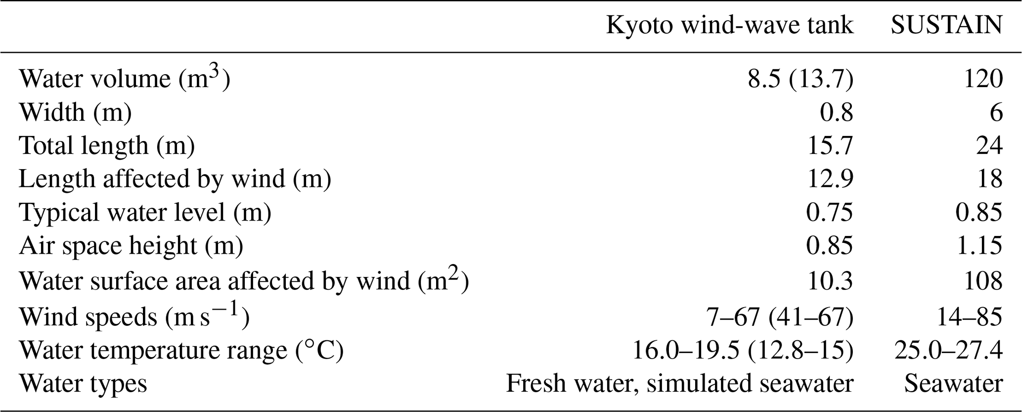
3.1.1 Water types

Due to technical limitations, seawater could not be used in the Kyoto High-Speed Wind-Wave Tank. There, one set of experiments was performed with tap water (referred to as fresh water or FW hereinafter). A second set of experiments was performed in Kyoto with a small amount of n-butanol added (approximately 700 mL) to the tap water, which modifies the bubble spectrum to better resemble that of seawater (Flothow, 2017). This second set of experiments will be referred to as the seawater model (SWM). The water used in the seawater model will be referred to as simulated seawater.

In the SUSTAIN tank, filtered seawater taken from Biscayne Bay was used. This set of experiments will be abbreviated as SW.

3.2 Mass balances for evasion experiments

A mass balance method is used to measure the gas transfer velocities in evasion-type experiments. In this approach, all gases are dissolved in the water and the water is mixed well by pumps before the wind is turned on. When the wind is turned on, the main flux is from the water volume to the air, and thus the concentration of the tracer in the water c_w decreases exponentially:

$$\begin{array}{}\text{(17)}& c_{\mathrm{w}}\left(t\right)=c_{\mathrm{w}}\left(\mathrm{0}\right)\exp \left(-k\cdot {\displaystyle \frac{A}{V_{\mathrm{w}}}}t\right),\end{array}$$

with the water volume V_w, the water surface A and the concentration at the start of the experiment c_w(0). In the Kyoto high-speed tank, the water lost due to spray was replaced with fresh water, which changes Eq. (17) to

$$\begin{array}{}\text{(18)}& c_{\mathrm{w}}\left(t\right)=c_{\mathrm{w}}\left(\mathrm{0}\right)\exp [-\left(k\cdot {\displaystyle \frac{A}{V_{\mathrm{w}}}}+{\displaystyle \frac{{\dot{V}}_{\mathrm{w}}}{V_{\mathrm{w}}}}\right)\cdot t],\end{array}$$

with the water loss rate ${\dot{V}}_{\mathrm{w}}/V_{\mathrm{w}}$. Thus, knowing the water volume, water surface area and the loss rate and measuring a concentration time series allows us to determine the gas transfer velocity k. A more thorough derivation of Eq. (18) can be found in Krall and Jähne (2014).

3.3 Gas concentration measurements, gas handling and tracers

In both experimental campaigns, a dual membrane inlet mass spectrometer (HPR-40 MIMS, Hiden Analytical, Warrington, UK) was used to measure the tracers' concentrations in water. The water extracted from the wind-wave tank was pumped along one of the inlet membranes where dissolved species diffuse through the membrane directly into the vacuum of the spectrometer where they are ionized and subsequently analyzed with respect to their concentrations. For some tracers, two mass-to-charge ratios were monitored with the MIMS, either because there are sufficiently high concentrations of different isotopes (e.g., Xe) or the tracer molecule is destroyed in the ionization process and forms multiple ions with different masses (e.g., DMS, DFB, HFB).

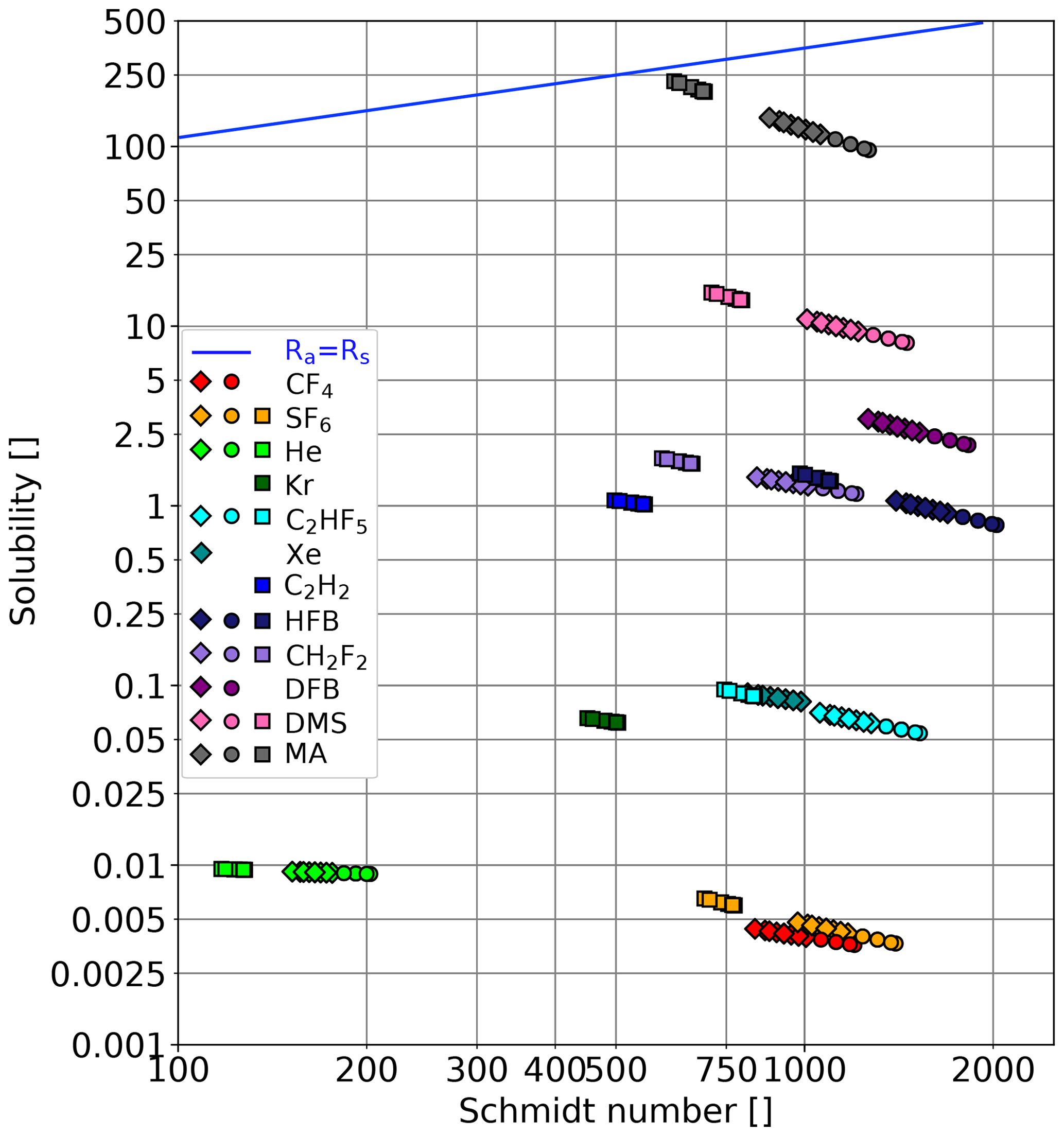
Figure 3 The solubility–Schmidt number combinations, for which the air-side resistance is equal to the water-side resistance, are shown as a blue line (Eq. 5 for a rough water surface). Diamonds: fresh water (Kyoto), circles: seawater model (Kyoto), squares: seawater (Miami). The variations in the Schmidt number and solubility result from the varying water temperatures used in the different experiments; see Table 1.

As mentioned in the previous section, before the start of the evasion experiment, all available gases were dissolved in the water and mixed well. For dissolving gases into the water, membrane contactors (SUSTAIN: Liqui-Cel 8×20 PVC, Kyoto: Liqui-Cel 4×13, Membrana 3M, Charlotte, NC, USA) were used. In Miami, the gases were dissolved directly into the water of the wind-wave tank, while in Kyoto the gases were first dissolved into a holding tank of approximately 7 m³. This water was then mixed into the main water volume of the wind-wave tank using pumps before the start of an experiment. Care was taken that the tracers were mixed into the water as homogeneously as possible. To achieve this, the pumps were kept on even after gas loading was finished, and the concentration was monitored. Only when the concentration was sufficiently stable the pumps were turned off and the experiment was started.

Table 2 Tracers used in this study. PFE: C₂HF₅, HFB: hexafluorobenzene, DFB: 1,4-difluorobenzene, DMS: dimethyl sulfide, MA: methyl acetate. Solubility and Schmidt number are given at 20 ^∘C for fresh water. Schmidt numbers were calculated from the kinematic viscosity (Kestin et al., 1978) and the diffusion coefficient is given in the respective citation.

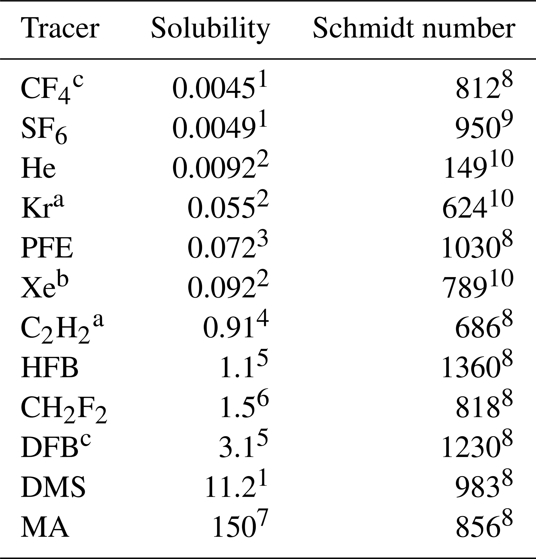
¹ (Warneck and Williams, 2012), ² (Abraham and Matteoli, 1988), ³ (Reichl, 1995), ⁴ (Sander et al., 2011), ⁵ (Hiatt, 2013), ⁶ (Maaßen, 1995), ⁷ (Fenclová et al., 2014), ⁸ (Yaws, 2014), ⁹ (King and Saltzman, 1995), ¹⁰ (Jähne et al., 1987). ^a Measured only in seawater. ^b Measured only in fresh water. ^c Measured only in fresh water and seawater model.

The tracers were chosen in this study to cover a wide range of solubilities and Schmidt numbers. Table 2 gives an overview of the tracers used sorted by their solubility. Due to technical and logistical reasons, not all tracers could be used in both facilities. Figure 3 shows the tracers in a Schmidt number–solubility diagram for all conditions encountered. The temperature dependency of the solubility and Schmidt number is apparent. Also shown is for which solubility–Schmidt number combination the air-side resistance equals the water-side resistance (αR_a=R_s; see also Eq. 5). To calculate the resistances, a rough and wavy water surface was assumed (i.e., $n=\mathrm{1}/\mathrm{2}$). Below this, αR_a=R_s line, the water-side resistance dominates; therefore, the tracers are called water-side controlled tracers. All tracers used in this study can be classified as water-side controlled tracers, with the exception of methyl acetate (MA), which is partially air-side controlled due to its relatively high solubility.

3.4 Wind speed measurements

3.4.1 Kyoto experiments

In the Kyoto tank, wind speeds were not recorded during the experiments. In Takagaki et al. (2012), streamwise and vertical air-side velocity fluctuations, measured using a laser Doppler anemometer and phase Doppler anemometer (LDA and PDA, Dantec Dynamics, Denmark) at a fetch of 6.5 m in the Kyoto tank, are given. They estimated the friction velocity $u_{\ast ,\mathrm{a}}$ by the Reynolds stress. Special care was taken that neither spray droplets nor the water film adhering to the side walls of the tank adversely affected the measurements (see also Komori et al., 2018).

Since we used the same wind generator settings as Takagaki et al. (2012), wind speed and friction velocities were taken from there with the exception of $u_{\ast ,\mathrm{a}}$ at the two highest wind speed settings. In Takagaki et al. (2012), $u_{\ast ,\mathrm{a}}$ at the highest wind generator setting (fan rotation number 800 rpm) was found to be smaller than $u_{\ast ,\mathrm{a}}$ at the second highest wind generator setting (fan rotation number 700 rpm), which might be due to a large measurement uncertainty due to intensive wave breaking. These values were extrapolated using a polynomial fit to the data reported in Takagaki et al. (2012), such that $u_{\ast ,\mathrm{a}}$ used here is strictly monotonically increasing with the wind speed setting as expected. These values of the friction velocity $u_{\ast ,\mathrm{a}}$ together with the wind speed values u₁₀ taken unaltered from Takagaki et al. (2012) were used to calculate the drag coefficient.

3.4.2 SUSTAIN experiments

A 3-D sonic anemometer (IRGASON, Campbell Scientific Inc., Logan, USA) was mounted in the test section of the SUSTAIN wind-wave tank at a fetch of 0.65 m and a height of 1.79 m above the tank bottom. The measured wind speeds were converted to the friction velocity $u_{\ast ,\mathrm{a}}$ and the wind speed u₁₀ using the parameterization for the drag coefficient given in Donelan et al. (2004) with the assumption of a logarithmic wind profile. Wind speed uncertainty was calculated from the device uncertainty as specified by the manufacturer as well as the variance of the wind speeds measured. Uncertainties found were on the order of 3 % to 4 %.

3.5 Bubble measurements

Bubble size distributions were measured in Kyoto using an optical bright field imaging technique (Mischler and Jähne, 2012; Flothow, 2017). A Nikon D800 digital SLR camera with a 200 mm f/4 AF-D macro lens looks perpendicular to the wind direction through the water into a purpose-built LED light source. Bubbles entrained in the water scatter the light such that the light no longer reaches the camera sensor, and the bubble appears as a dark circle. Out-of-focus bubbles have a blurry edge, which is used to estimate the 3-D volume the bubbles are in the 2-D images taken by the camera by depth from focus (Jähne and Geißler, 1994). Two bubble imaging systems were operated during the measurements in Kyoto: one at a fetch of 3 m and the second one at 8 m fetch, approximately 30 cm below the water surface. Calibration and data evaluation is described in detail in Flothow (2017).

Figure 4 Relationship between the wind speed at 10 m height, u₁₀, and the water-side friction velocity (a) and the drag coefficient calculated using Eq. (16) (b). Lighter colors mark conditions where the friction velocity was approximated; see Sect. 3.4.

4 Results and discussion

4.1 Wind speeds and friction velocities

The relationship between the water-sided friction velocities $u_{\ast ,\mathrm{w}}$ and the wind speeds in 10 m height u₁₀ at which the gas transfer velocities were measured in this study is shown in Fig. 4a. A clear change in the steepness of the relationship can be seen at a wind speed of approximately 33 m s⁻¹, as indicated by the gray line. The wind speed of 33 m s⁻¹ corresponds to a friction velocity of about 6 cm s⁻¹. Also, the drag coefficient (C_D; Fig. 4b) has a maximum at this wind speed before it levels off.

4.2 Bubble surface area

Up to now, bubble measurements were evaluated only for the Kyoto facility. From the bubble concentration measurements, the total bubble surface was computed and plotted in Fig. 5 as a dimensionless area in relation to the flat free water surface area, A_b∕A_s. The uncertainties are quite high, because bubbles where measured only at one depth (Sect. 3.5). But still a few important findings can be stated.

1. The bubble surface area strongly increases with the friction velocity ($\propto u_{\ast ,\mathrm{w}}^{\mathrm{3}}$ to $\propto u_{\ast ,\mathrm{w}}^{\mathrm{4}}$) in all facilities and for fresh water and seawater.

2. For fresh water, the bubble surface area almost reaches the same area as the flat free surface at the highest wind speeds.

3. In the modeled seawater, the bubble surface area is about an order of magnitude larger than in fresh water. At higher friction velocities, especially with the seawater model, the bubble clouds get very dense, resulting in a systematic underestimation of the bubble surface area. Therefore, the true bubble surface area at the highest wind speed is very likely larger than the measured surface area of about 4 times the area of the flat free water surface.

4. The bubble surface area shows a clear trend to increase with fetch. Also shown in Fig. 5 are measurements performed at 28 m fetch (Marseille tank) and quasi-infinite fetch in the annular wind-wave facility, the Heidelberg Aeolotron in addition to the measurements in Kyoto at 3 and 8 m fetch. Roughly, the same bubble surface area is obtained at about half the friction velocity in the Aeolotron as compared to 3 m fetch in the Kyoto facility. With the modeled sea water, the bubble surface area becomes equal to the flat free surface area at a friction velocity just above 4 cm s⁻¹, while this value is reached in the Kyoto facility only at a friction velocity of about 8 cm s⁻¹. This finding is important when extrapolating laboratory results to the field and will be discussed further in Sect. 4.5.2.

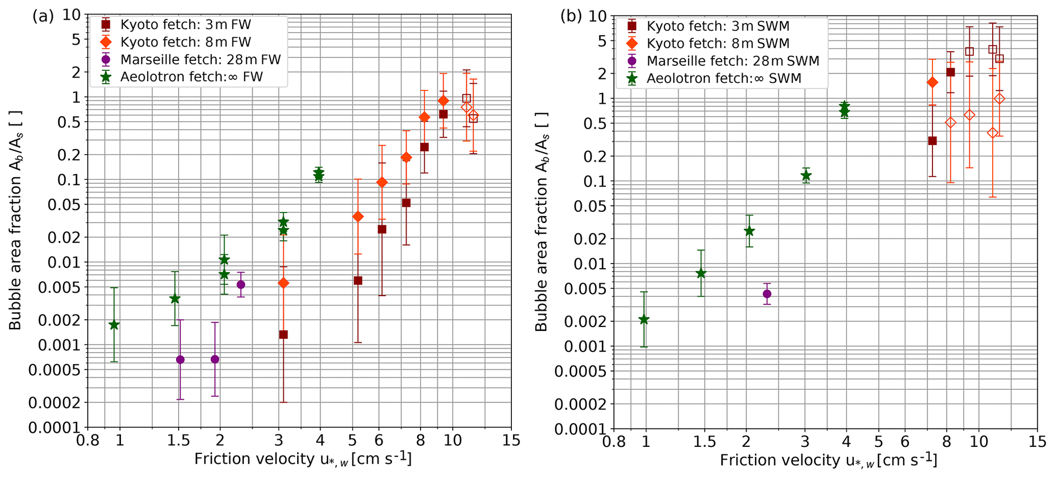
Figure 5 Bubble surface area per water surface area measured in fresh water (a) and seawater modeled by adding butanol to fresh water (b) Kyoto: 3 and 8 m fetch, with the camera installed approximately 30 cm below water surface at rest; Marseille Luminy: 28 m fetch, with the camera installed at approximately 50 cm below water surface at rest; Aeolotron Heidelberg: infinite fetch, with the camera installed at 10 evenly spaced positions between 0.5 and 36.5 cm below the water surface. At the highest wind speeds, the density of the bubbles is so large that the intensity of the illumination that reaches the camera is reduced by up to 75 %, which leads to a systematic underestimation of the bubble surface area. Conditions likely affected by this are marked with an open symbol. Figure reproduced from data by Flothow (2017).

4.3 Measured gas transfer velocities

Figure 6 shows the measured gas transfer velocities k_meas in dependency of the water-sided friction velocity $u_{\ast ,\mathrm{w}}$ for three different measurement conditions: (a) fresh water in Kyoto, (b) seawater model in Kyoto and (c) seawater in Miami. Gas transfer increases strongly with the wind speed for all tracers. Beyond a friction velocity of approximately 6 cm s⁻¹, the increase is significantly steeper.

The tracer with the highest solubility, methyl acetate (MA), shows a transfer velocity significantly lower than for the other tracers for all wind speeds and all water types. This reduction in the gas transfer velocity confirms the existence of an additional air-side resistance for this tracer; see Sect. 2.1. Due to this additional air-side resistance, MA will be excluded in the following discussion. From Fig. 6, it is also evident that He has a much higher transfer velocity than the other tracers for all wind speeds. This is caused by its significantly higher diffusion coefficient corresponding to a low Schmidt number, while all other tracers vary in the Schmidt number by at most a factor of 2; see Table 2.

Figure 6 also shows dependencies of the form $k_{\mathrm{meas}}\propto u_{\ast ,\mathrm{w}}^x$ with a variable exponent x. Clearly, the functional dependency between k_meas and $u_{\ast ,\mathrm{w}}$ dramatically changes at a friction velocity of around 6 cm s⁻¹, indicating a new regime starting at this friction velocity. This finding is in good agreement with the earlier measurements of Iwano et al. (2013) and Krall and Jähne (2014), who also found a transition to a much steeper increase at 33–35 m s⁻¹ (u₁₀). Also, this wind speed coincides with the change in the $u_{\ast ,\mathrm{w}}\left(u_{\mathrm{10}}\right)$ relationship discussed in Sect. 4.1.

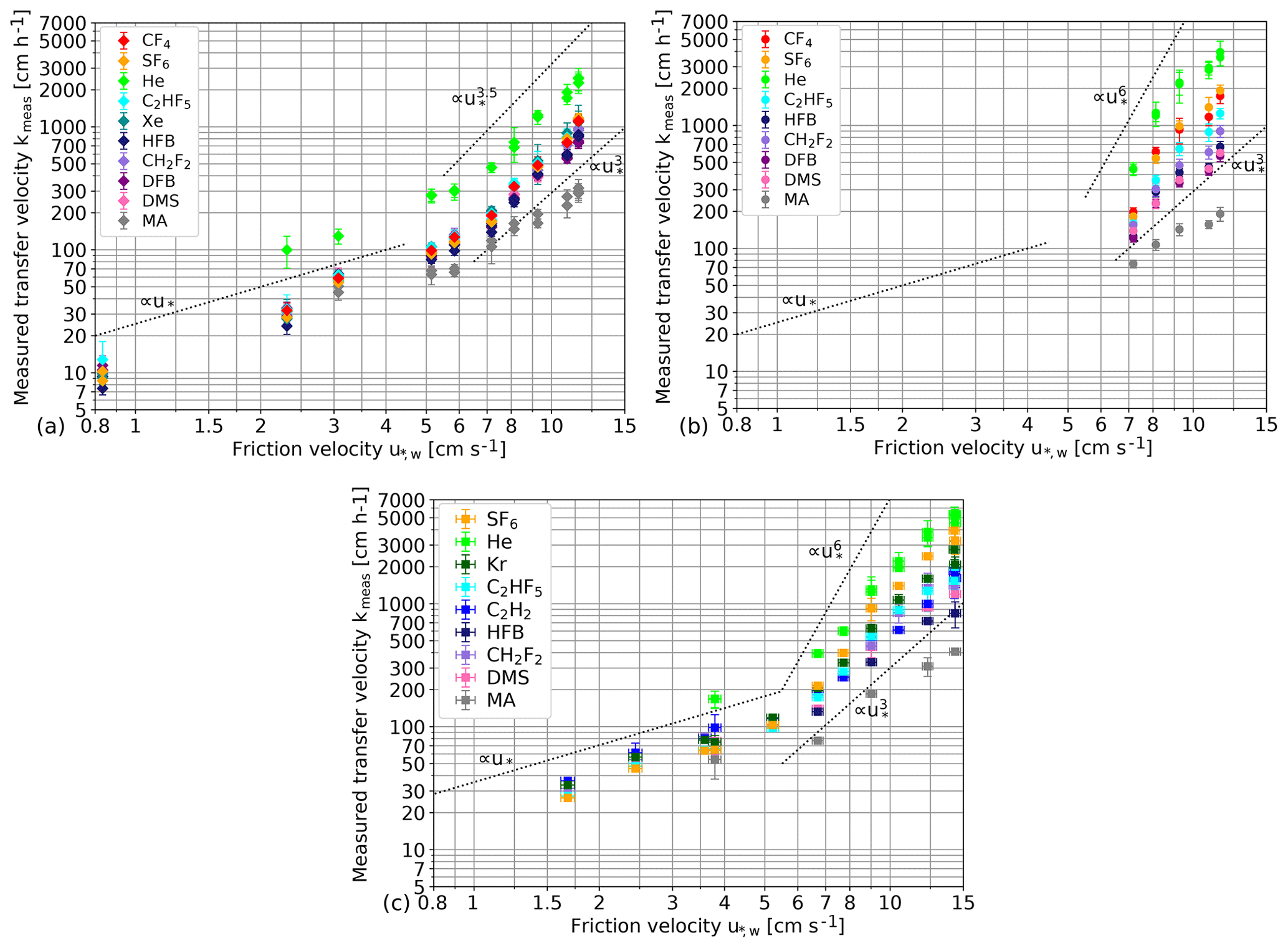
Figure 6 Measured gas transfer velocities k_meas in fresh water in Kyoto (a), in the seawater model in Kyoto (b) and in seawater in Miami (c). Tracers in the legend are sorted by increasing solubility. As a visual guide, lines showing exponential proportionalities between the transfer velocity and the friction velocities to varying powers are shown.

A closer look at the fresh water transfer velocities (Fig. 6a) reveals an unexpected result. Even for high wind speeds, all tracers (except He and MA) have transfer velocities within a very narrow band, even though their solubility differs by several orders of magnitude. This is a clear indication that transfer through closed bubble surfaces is much slower than the transfer through the water surface for fresh water even at the highest wind speeds.

In seawater and in simulated seawater (Fig. 6b and c), a clear spacing between the transfer velocities of tracers with different solubilities at high wind speeds can be seen. This means that bubble-induced gas transfer does play a role for seawater.

4.4 Separation of gas transfer across the free surface and bubbles

Once bubbles influence air–sea gas transfer, a separation of the different contributing mechanisms is required. Because of the additional influence of solubility, it is not possible to simply apply Schmidt number scaling. This is why the model combining gas transfer across the free water surface and bubble surface was developed in Sect. 2.2; see Eq. (11). Because all measurements were made at high wind speeds with clean water, the Schmidt number exponent was fixed to 0.5. Then, three unknown parameters remain for each measuring condition:

• The first parameter is the transfer velocity across the free water surface at a Schmidt number of 600, k_s,600.

• The second parameter is the limiting or maximum transfer velocity across the closed-bubble surfaces at a Schmidt number of 600, k_c,600. It is reached for gases with a solubility α≪α_t.

• The last parameter is the transfer velocity associated with the bubble volume flux density, k_r. For high solubility (α≫α_t), the bubble-mediated gas transfer velocity is k_r∕α; compare Eq. (8).

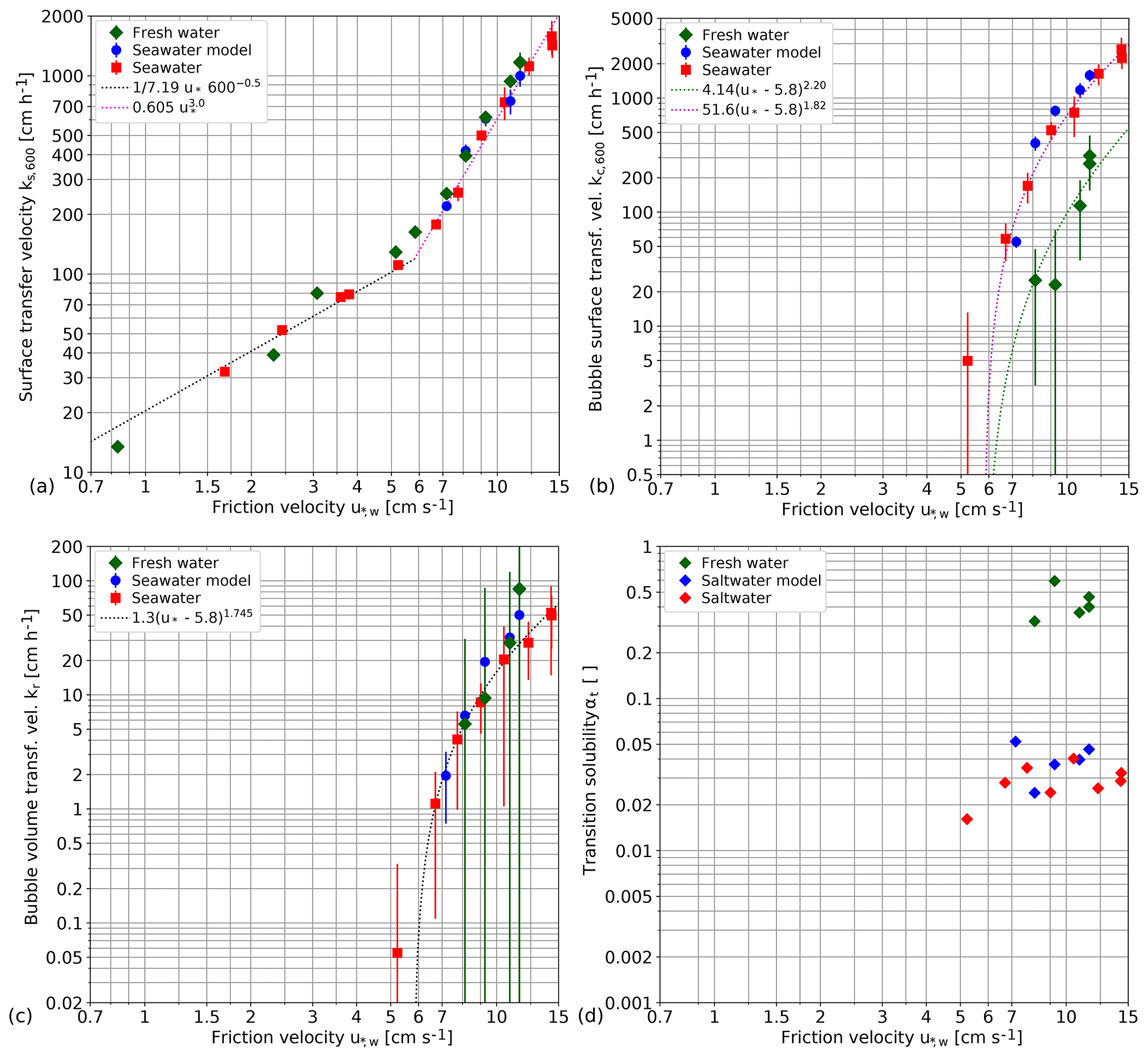
Figure 7 Fitted contribution of the different components to the gas transfer velocity: (a) surface transfer velocity k_s,600, (b) bubble surface transfer velocity k_c,600 and (c) the bubble volume k_r as a function of the water-side friction velocity in double-logarithmic presentation. Please note the different vertical scales. The graphs include error bars of the fitted parameters. In addition, the transition solubility α_t computed according to Eq. (9) is shown in panel (d) without error bars.

Because of the multi-tracer approach with more than three tracers covering a wide range of solubilities, it is possible to retrieve all three parameters of the model (Eq. 11) for each measuring condition separately and thus to separate the gas transfer across the free water surface from the bubble-induced gas transfer. In addition, the transition solubility α_t can be computed according to Eq. (9). The model Eq. (11) was fitted to the data using a least squares algorithm with the free parameters k_s,600, k_r and k_c,600. More information on the algorithm to retrieve those parameters can be found in the Supplement. MA was excluded from the fit due to its additional air-side resistance. Also, He had to be excluded. Including He led to unrealistically low transition solubility of below 0.001. One possible reason for this is the high diffusion coefficient of He and the resulting fast gas transfer from water into the bubbles, which might deplete the He concentration in the water between the bubbles inside bubble clouds. This effect has been observed and described before by Woolf et al. (2007). Another explanation is spray-induced gas transfer, which could limit the gas transfer velocity of tracers with high diffusivity as discussed in Sect. 2.3.

Also, as a further quality criterion, the fit was required to obey

$$\begin{array}{}\text{(19)}& k_{\mathrm{c},\mathrm{600}}\le k_{\mathrm{meas},\mathrm{T}}{\left({\displaystyle \frac{S{c}_{\mathrm{t}}}{\mathrm{600}}}\right)}^{\mathrm{0.5}}-k_{\mathrm{s},\mathrm{600}},\end{array}$$

for the tracers T = [SF₆,CF₄]. This was achieved by iteratively narrowing the allowed parameter space of the parameter k_c,600. Equation (19) describes the highest physically reasonable k_c,600 (see also Eq. 12). At each measuring condition, the regression with three free parameters was performed with 5–14 measured transfer velocities. For some tracers, the concentrations of two different ions of the same tracer were analyzed with the MIMS, which allowed the measurement of two transfer velocities per tracer for a single wind speed condition; see Sect. 3.3.

The mean (median) deviation between the measured and the modeled transfer velocity is 7.4 % (6.3 %) of the measured transfer velocity. Out of a total of 242 pairs of measured and modeled values, only 22 deviate by more than 15 %. The maximum deviation found was 31.2 % (acetylene in seawater at u₁₀=62.9 m s⁻¹). This indicates that the regression model is in good agreement with the measured data. Detailed plots comparing measured and modeled values can be found in the Supplement.

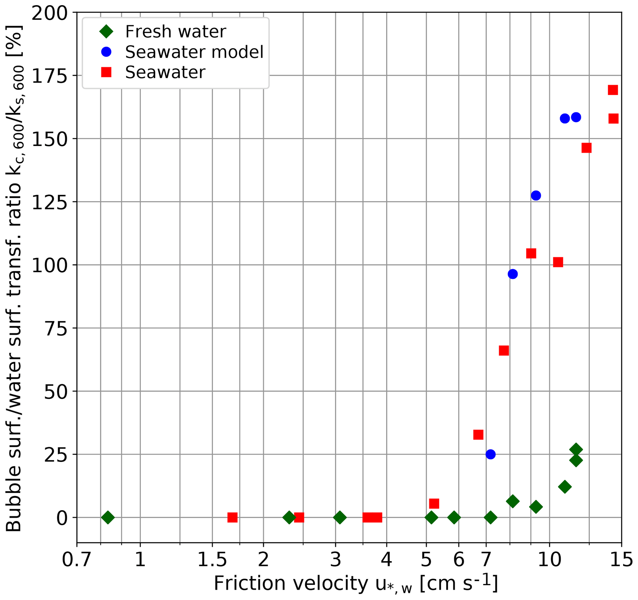
Figure 8 Ratio of k_c,600 to k_s,600, i.e., the bubble-induced gas transfer velocity in the limit of low solubility to the gas transfer velocity at the free surface in relation to the friction velocity, given in percent of the gas transfer velocity at the free surface.

Figure 7 shows the resulting fitted parameters (k_s,600, k_r and k_c,600) and the calculated transition solubility (α_t; see Eq. 9). The bubble-related parameters (k_r and k_c,600) are found to be zero for friction velocities below 5.8 cm s⁻¹ for fresh water and seawater. No experiments below 7 cm s⁻¹ were performed for the seawater model. The separation of the gas transfer velocity into its different components gives a detailed insight into the mechanisms of air–sea gas transfer at high wind speeds with unexpected results:

• The gas transfer velocity across the free water surface k_s,600 normalized to a Schmidt number of 600 (Fig. 7a) clearly shows a transition to a much steeper increase of the transfer velocity with the friction velocity from $\propto u_{\ast ,{\mathrm{w}}^{\mathrm{1}}}$ to $\propto u_{\ast ,\text{w}}^{\mathrm{3.0}}$ beyond a friction velocity of about 5.8 cm s⁻¹. It is a substantial effect, resulting in an about 10-fold gas transfer velocity if the water-side friction velocity is increased by a factor of 2 from 6 to 12 cm s⁻¹. This substantial increase of the gas transfer velocity is not related to bubble-induced gas transfer at all and thus valid for all water-side controlled gas tracers independent of the solubility. It is not unexpected that there is no significant difference between seawater and fresh water, because the hydrodynamic conditions do not depend on the salt content of the water, and the normalization of the transfer velocity to a Schmidt number of 600 already takes the small change of the kinematic viscosity between seawater and fresh water into account. It is more surprising that there is no significant difference between the Kyoto and SUSTAIN facilities although they differ significantly in lengths (15.7 m versus 24 m) and width (0.8 m versus 6 m).

• The bubble-induced gas transfer velocity k_c,600 could only be measured after the transition to a much steeper increase of the gas transfer velocity at the surface beyond a friction velocity of 5.8 cm s⁻¹. (Fig. 7b and c). The maximum bubble-induced gas transfer velocity in the limit of low-solubility k_c,600 increases even more steeply (Fig. 7b). For all fresh water conditions studied, bubble-induced gas transfer remains much smaller than the gas transfer at the free water surface. For seawater, however, k_c,600 is an order of magnitude higher and surpasses k_s,600 at a friction velocity of about 8 cm s⁻¹. At the highest wind speed, it is about 1.7 times larger than at the free surface (Fig. 8). The about 10-fold larger bubble-induced gas transfer velocity for seawater than for fresh water in the limit of low solubilities is in good agreement with the measured bubble surface, as presented in Sect. 4.2.

• The bubble volume flux related transfer k_r for high solubilities is not significant at all (Fig. 7c). It is also not unexpected that there is no significant difference between seawater and fresh water, because in this limit, bubble-induced gas exchange is controlled by the bubble volume flux. It can be expected that the gas volume submerged per breaking wave does not depend on the salt content, because this depends only on the geometry and dynamics of wave breaking.

• The transition solubility α_t is different for seawater and fresh water. In seawater, many more small bubbles are generated, which stay longer in the water and form a significantly larger surface. This is why seawater is much more effective in bubble-induced gas transfer for low solubilities. Therefore, for seawater, the transition from surface to volume controlled bubble-mediated gas transfer is shifted to lower solubilities of around 0.03 from values of about 0.4 for fresh water.

  Within the measurement accuracy, no difference was found between seawater and simulated seawater. Thus, not only the absolute values of bubble-induced gas transfer (Fig. 7b and c) but also the transition solubility is correctly reproduced when using traces of n-butanol in fresh water to simulate the effect of seawater on bubble generation and its effects on air–sea gas transfer. This greatly simplifies laboratory experiments.

  In his bubble tank experiment, Mischler (2014) found similar transition values: for fresh water 0.23 and for saltwater 0.06 at the conditions shown in Fig. 2. The small deviations are not surprising, because in a bubble tank without wind, where the breaking waves are simulated by a jet, the turbulence in the water certainly is different.

4.5 Comparison with field measurements

4.5.1 Bubble-induced gas transfer

At first glance, the most striking result is the negligible contributions of bubbles to gas transfer up to wind speeds of 33 m s⁻¹. There is evidence that bubbles contribute to air–sea gas exchange at much lower wind speeds at the ocean surface. Both Blomquist et al. (2017) and Bell et al. (2017) found significantly higher gas transfer velocities for carbon dioxide than for DMS and attributed this to bubble-induced gas transfer (Fig. 9). However, doubts remain. First, the field experiment by Zavarsky et al. (2018) did not show a significant difference between DMS and CO₂ gas transfer velocities (Fig. 9). Secondly, CO₂ gas transfer velocities measured by eddy covariance techniques are generally about a factor of 2 higher than gas transfer velocities measured with the dual tracer technique using ³He∕SF₆ (Garbe et al., 2014, Fig. 2.10) when scaled to the same Schmidt number. This should not be the case, because both ³He and SF₆ have much lower solubilities than CO₂ and consequently should show a higher transfer velocity than CO₂, not a much smaller one.

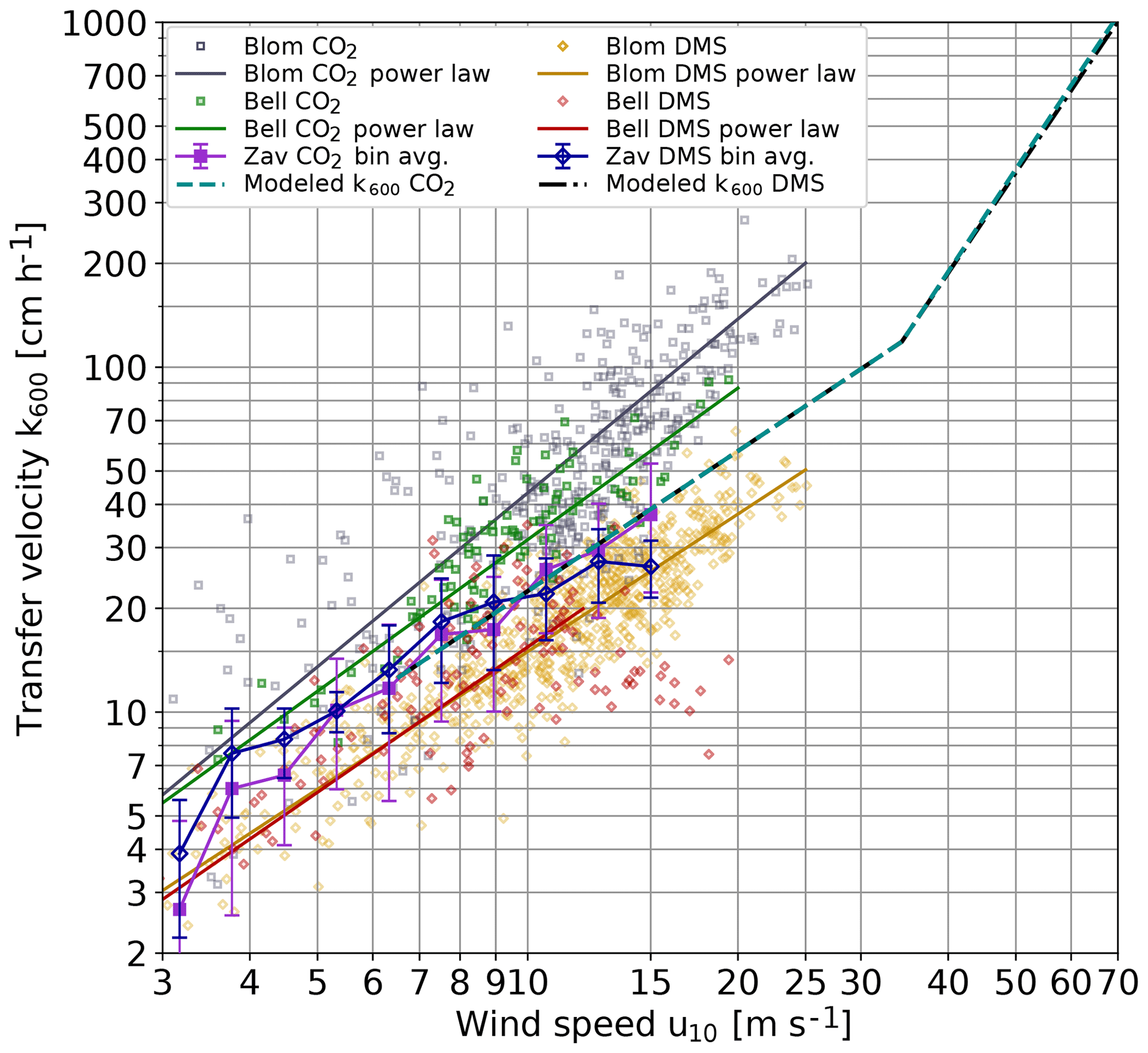
Figure 9 Comparison of DMS and carbon dioxide gas transfer velocities in a double-logarithmic representation: eddy covariance measurements from the High Wind Speed Gas Exchange Field Study (HiWinGS) by Blomquist et al. (2017) (Blom) including their k(u₁₀) parameterizations. Also shown are the CO₂ and DMS transfer velocities measured by Zavarsky et al. (2018) (Zav) and those reported in Bell et al. (2017) (Bell). For the Bell data, power laws of the form $a{u}_{\mathrm{10}}^n$ taken from Brumer et al. (2017) are shown. The output of the model presented in this paper for CO₂ and DMS is also shown.

4.5.2 Wave age dependency

But even if the bubble-mediated gas transfer is estimated correctly by combined DMS/CO₂ measurements, this does not necessarily contradict the laboratory measurements, because of the very different wave ages between linear wind-wave tunnels and the ocean. The bubble surface area measurements reported in Sect. 4.4 and Fig. 5b show indeed larger bubble surface areas with increasing fetch at the same wind speed. In the Heidelberg Aeolotron with infinite fetch, the same bubble surface area occurs at about half the wind speed than in the short-fetch Kyoto facility.

Therefore, it appears logical that wave breaking in the ocean could be more intense than in a short-fetch wind-wave tank and thus would start to become significant at considerably lower wind speeds. This is supported by the estimation of air entrainment by breaking waves by Deike et al. (2017). They estimated maximum air entrainment velocities V_a=k_r up to about 50 cm h⁻¹, as we did (Fig. 2c), but already at much lower wind speeds.

However, with the current state of knowledge, it is not possible to draw definitive conclusions. As pointed out by Brumer et al. (2017), some field measurements showed a significant wave age dependency others did not. There are also contradictory theoretical and semi-empirical models, as the discussion about the findings by Deike et al. (2017); Deike and Melville (2018) in the last paragraph of Sect. 2.2 showed.

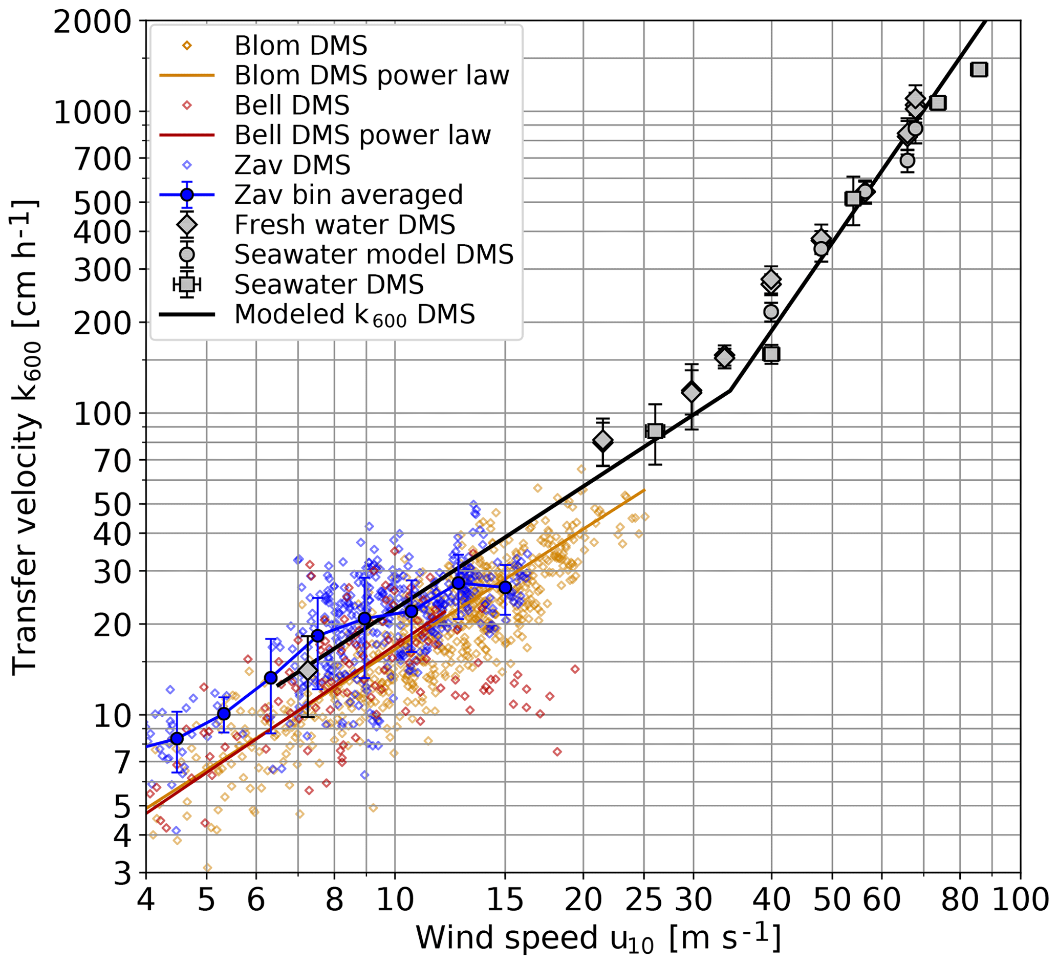
Figure 10 Measured transfer velocities of DMS, scaled to k₆₀₀, compared to previous field studies. Bell: Bell et al. (2017); Blom: Blomquist et al. (2017); Zav: Zavarsky et al. (2018).

4.5.3 DMS gas transfer

One set of eddy covariance measurements (Bell et al., 2013, 2015) found a decrease of the gas transfer for wind speeds higher than approximately 12 m s⁻¹, while all other field measurements do not show this effect (Fig. 10) The measurements presented here do not show such an effect (Fig. 10). On the contrary, beyond a wind speed of about 33 m s⁻¹, the transfer velocity shows the same transition to a much steeper increase as all other tracers used. Thus, the transfer of DMS across the air–water interface in fresh water and seawater is just the same as for all other gases and volatile tracers, and theories about an attenuated Henry's law constant for DMS (Vlahos and Monahan, 2009) are most likely not correct.

4.5.4 Very high wind speeds

The most interesting and novel result is the steep increase of the gas transfer velocity beyond 33 m s⁻¹ to values exceeding 1000 cm h⁻¹. In this wind speed range, the comparison with only two transfer velocities estimated in a field measurement with oxygen is possible (McNeil and D'Asaro, 2007). The modeled values of the oxygen gas transfer velocities were calculated according to Eq. (11) and the model equations contained in the Supplement. It is interesting to see how close our wind-wave tank data are to the field data (Fig. 11). This clearly means that the mechanisms causing this steep increase in the laboratory in this wind speed range are also relevant for field conditions.

4.5.5 From lab to ocean conditions

It is evident that gas transfer cannot be directly transferred from a wind-wave flume to the ocean. This is just as wrong as using empirical gas transfer–wind speed relations from a collection of field experiments, because parameters other than wind speed also influence gas transfer. This is not just the sea state as discussed above but also the influence of surface active material at the water surface (Frew, 1997; Cunliffe et al., 2013; Nagel et al., 2019). It is exactly this multitude of parameters influencing air–sea gas transfer which makes it so difficult to identify and quantify the mechanisms. Here, laboratory studies can play an important role. Laboratory measurements are generally much more precise and accurate than any current field measuring techniques. It is possible to use many more tracers simultaneously. Also, it is easy to perform systematic studies.

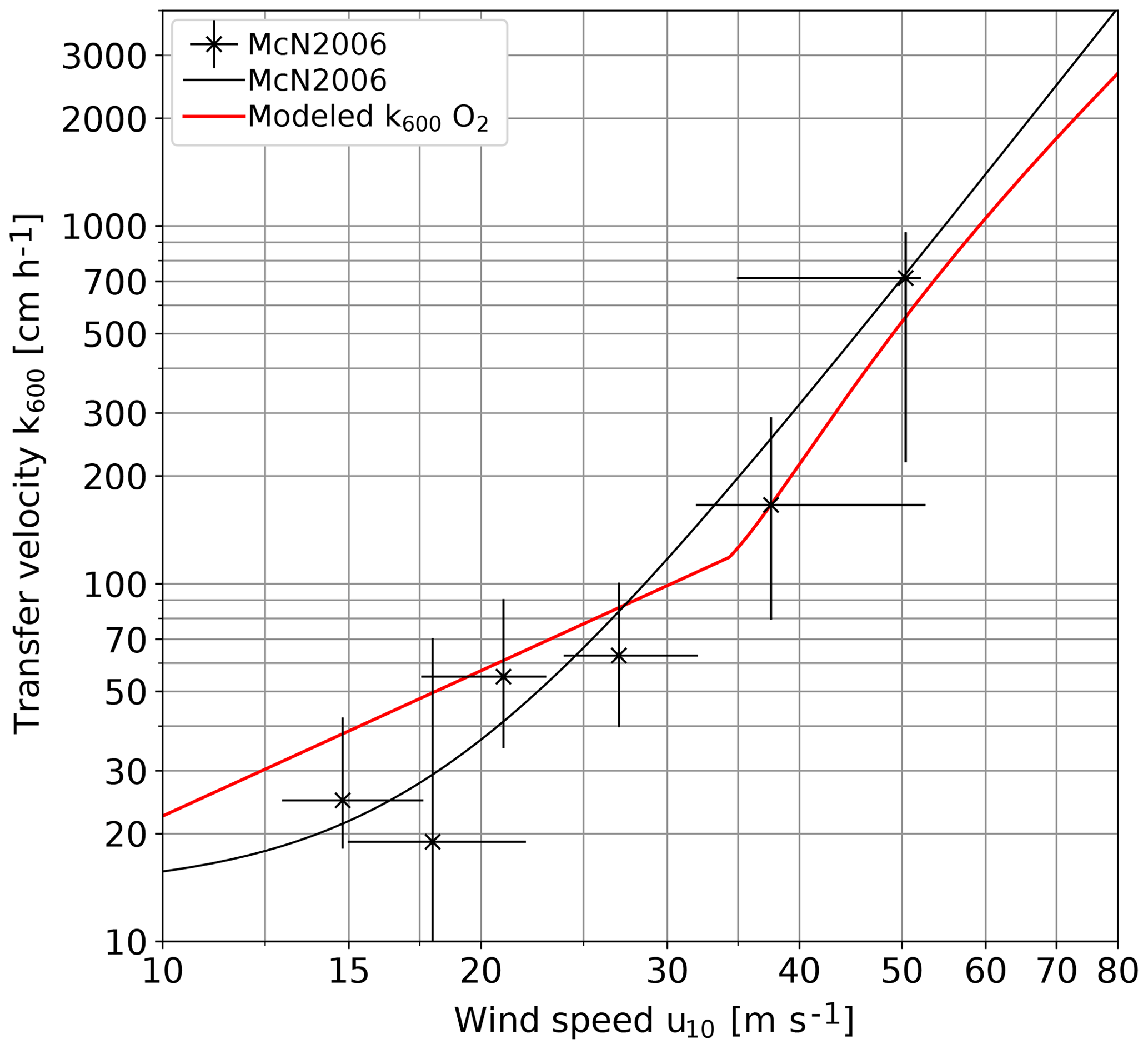
Figure 11 Comparison of oxygen gas transfer velocities inferred from the lab measurements presented in this paper with the field data by McNeil and D'Asaro (2007); both are Schmidt number scaled to k₆₀₀.

There were two serious limitations in the past: the limited wind speeds and low-fetch conditions. The first limitation is already gone with the Kyoto High-Speed Wind-Wave Facility and the Miami SUSTAIN Facility. The second limitation can be overcome in annular facilities such as the Heidelberg Air-Sea Interaction Facility, the Aeolotron. It is not required to perform perfect replications of ocean conditions. This will not be possible anyway. It is just necessary to describe the findings with physically based models that cover all important mechanisms and then to adapt the parameters to conditions at the ocean surface.

One may argue that large breaking waves cannot be simulated adequately in wind-wave tunnels. However, the basic physical mechanisms seem to be remarkably scale independent. Air entrainment from breaking waves is a good example of this. Su and Cartmill (1995) measured bubble distributions and void fractions in a 90 m long, 3.36 m deep and 3.66 m wide wave channel with large mechanically generated breaking waves using fresh water and artificial seawater. They found an about 10-fold larger bubble surface area in sea water than in fresh water but no significant change in the void fraction, which agrees well with our findings in much shallower facilities. In a small-scale tipping-bucket experiment, Carey et al. (1993) compared air entrainment in seawater and fresh water and found, as we did in our experiments, that the volume flux of air entrainment is about the same for both water types.

5 Conclusions and outlook

With multi-tracer gas exchange experiments in two high-speed wind-wave tanks, it was possible to separate the mechanisms of air–sea gas transfer into its different components, transfer across the free water surface, transfer across closed bubble surfaces and transfer associated with the bubble volume flux density.

In the short-fetch tanks, a steep increase of the transfer velocity across the free surface was found beyond wind speeds of 33 m s⁻¹ (friction velocity in water 5.8 cm s⁻¹) increasing the transfer velocity corrected to a Schmidt number of 600 from 110 cm h⁻¹ to a maximum measured value of about 1600 cm h⁻¹. This part of the gas transfer is the same in fresh water and seawater. It is obvious that a new regime is established at wind speeds beyond 33 m s⁻¹, which is governed by the intense turbulent mixing and permanent rapid disruption of the surface. The detailed mechanisms causing the steep increase of the gas transfer velocity at high wind speeds are still unclear and require further investigations. Because this effect is clearly not caused by gas transfer through closed bubble surfaces, it can be explained as either significantly enhanced turbulence at the water surface, or a significantly enlarged surface area for the exchange processes, or a combination of both. Many processes must be considered at highest wind speeds, including the generation of steep small-scale surface waves, the fragmentation of wave crests where the bag-breakup mechanism is dominant (Troitskaya et al., 2017), the effects of high-speed spray and spume droplets plunging into the water surface again and the effects of bursting bubbles. The finding of the relatively low transfer velocity for He at the highest wind speed (Sect. 4.4) is a first indication that rapid surface fragmentation processes play an important role, but further studies are required. It can be expected that this new regime with a steep increase of the gas transfer velocity for all tracers independent of solubility exits with the same type of mechanisms at sea. This regime still has to be explored at sea.

Bubble-mediated gas transfer might differ between the lab measurements presented here and field measurements, because of the wave age or fetch dependency. As has been discussed in detail in Sect. 4.5.2, the wave age dependency of air–sea gas transfer is not well known and urgently requires more detailed investigations. Only then will it be possible to quantify the bubbles' influence on air–sea gas exchange in the field and, more specifically, to which extent an important tracer such as carbon dioxide will be influenced by bubble-induced gas transfer.

In the laboratory experiments reported here, bubbles do not significantly contribute to the gas transfer velocity of tracers with a solubility of around 1 and higher (such as CO₂) even at the highest wind speeds.

In field experiments, it remains very difficult to reveal the mechanisms of air–sea gas transfer because there are not enough tracers available simultaneously to span the necessary wide range of tracer solubility and diffusivity and because systematic studies scanning all relevant environmental conditions are very demanding and time consuming. As this study has shown, systematic and well-designed wind-wave tank experiments have more potential to reveal the mechanisms of the gas transfer processes. This also opens up the opportunity to predict transfer velocities under field conditions. In particular, future high-wind-speed gas transfer studies in the annular Heidelberg Aeolotron with infinite fetch have the potential to narrow the “fetch gap” between the laboratory and the field.

The Heidelberg Aeolotron with infinite fetch has the potential to narrow the “fetch gap” between the laboratory and the field.