the Creative Commons Attribution 4.0 License.
the Creative Commons Attribution 4.0 License.
 | 13 Dec 2019
Rotation of floating particles in submesoscale cyclonic and anticyclonic eddies: a model study for the southeastern Baltic Sea
Victor Zhurbas
Germo Väli
Natalia Kuzmina
We hypothesized that the overwhelming dominance of cyclonic spirals on satellite images of the sea surface could be caused by some differences between the rotary characteristics of submesoscale cyclonic and anticyclonic eddies. This hypothesis was tested by means of numerical experiments with synthetic floating Lagrangian particles embedded offline in a regional circulation model of the southeastern Baltic Sea with very high horizontal resolution (0.125 nautical mile grid). The numerical experiments showed that the cyclonic spirals can be formed from both a horizontally uniform initial distribution of floating particles and from the initially lined-up particles during an advection time of the order of 1 d. Statistical processing of the trajectories of the synthetic floating particles allowed us to conclude that the submesoscale cyclonic eddies differ from the anticyclonic eddies in three ways favoring the formation of spirals in the tracer field: they can be characterized by (a) a considerably higher angular velocity, (b) a more pronounced differential rotation and (c) a negative helicity.
- Article
(15554 KB) - Full-text XML
- BibTeX
- EndNote


Spiral structures that can be treated as signatures of submesoscale eddies are a common feature on synthetic aperture radar (SAR), infrared and optical satellite images of the sea surface (e.g., Munk et al., 2000; Laanemets et al., 2011; Karimova et al., 2012; Ginzburg et al., 2017). The spirals are broadly distributed in the World Ocean, 10–25 km in size and overwhelmingly cyclonic (Munk et al., 2000). Walter Munk (Munk, 2001) has summarized the formation mechanism of the spirals as follows: “Under light winds favorable to visualization, linear surface features with high surfactant density and low surface roughness are of common occurrence. We have proposed that frontal formations concentrate the ambient shear and prevailing surfactants. Horizontal shear instabilities ensue when the shear becomes comparable to the Coriolis frequency. The resulting vortices wind the linear features into spirals.” Horizontal shear instabilities were shown to favor cyclonic shear and cyclonic spirals for different reasons (Munk et al., 2000).
The submesoscale flows are the upper ocean layer flows with a horizontal length scale of the order of 0.1–10 km that are characterized by a Rossby number (the ratio of relative vertical vorticity to the Coriolis frequency) and a Richardson number (the ratio of the squared buoyancy frequency to the squared vertical shear) of the order of unity, as well as by a conspicuous asymmetry of the relative vertical vorticity distribution with a tail of enhanced positive (cyclonic) vorticity values (Thomas et al., 2008; McWilliams, 2016). Submesoscale processes play an important role in turbulence and mixing of the upper ocean layer (Fox-Kemper et al., 2008, 2011; Thomas et al., 2008; McWilliams, 2016). While horizontal shear or barotropic instability is one possible mechanism for generating submesoscale eddies (Munk's hypothesis), more recent studies have shown that mixed-layer baroclinic instabilities (Haine and Marshall, 1998) are a more plausible explanation for the observed submesoscale vortices (e.g., Eldevik and Dysthe, 2002; Boccaletti et al., 2007; Dewar et al., 2015; Molemaker et al., 2015; Buckingham et al., 2017).
Submesoscale structures and the associated instabilities were simulated using high-resolution circulation models in various areas of the World Ocean such as the California Current System (Capet et al., 2008; Dewar et al., 2015; Molemaker at al., 2015), the Gulf Stream (Gula et al., 2016) and the Gulf of Mexico (Barkan et al., 2017). Similarly, high-resolution circulation models with a horizontal grid of less than 0.6 km were implemented to also study submesoscale dynamics in the Baltic Sea (Vankevich et al., 2016; Väli et al., 2017, 2018; Vortmeyer-Kley et al., 2019; Zhurbas et al., 2019; Onken et al., 2019).
Idealized, submesoscale-permitting model experiments (Brannigan, 2016; Brannigan et al., 2017) have shown that long spiral-like filaments in the surface pattern of a tracer field can be linked to the alternation of upwelling–downwelling cells with a transverse wavelength of the order of 1 km in the mixed layer of a differentially rotating eddy caused by submesoscale instabilities, namely the symmetric instability (e.g., Thomas et al., 2013). The submesoscale upwelling can bring nutrients from the thermocline to the mixed layer, thereby increasing the biological productivity (Brannigan, 2016). An interplay between mesoscale dispersion and submesoscale clustering of flotsam was studied by field observations of a large number of surface drifters deployed within a test area in the Gulf of Mexico (D'Asaro et al., 2018). More than half of the surface drifter array covering km2 aggregated into a 60×60 m2 region within a week, a factor of more than 105 decrease in area, before slowly dispersing. The convergence occurred at submesoscale density fronts with vertical cyclonic vorticity ζ exceeding the planetary vorticity f: . The lining up of uniformly spaced synthetic floating particles at submesoscale density fronts with high cyclonic vorticity was simulated using a submesoscale-permitting model in the Gulf of Finland (Väli et al., 2018). Aggregation of simulated floating particles at the edges of anticyclonic eddies as applied to biomass redistribution was explored in Samuelsen et al. (2012). An attempt to quantify the associated systematic changes to the density of particles in terms of so-called finite-time compressibility was made in Kalda et al. (2014).
Spirals in the southeastern Baltic Sea were repeatedly observed in infrared (e.g., Zhurbas et al., 2004; Ginzburg et al., 2017), SAR (Karimova et al., 2012) and optical (e.g., Karimova et al., 2012; Ginzburg et al., 2017) images. The most illustrative optical images have been encountered in summer when the spirals become visualized by the cyanobacteria blooms. Submesoscale processes can redistribute cyanobacteria mass to form both spiral-like patches of enhanced concentration and cyanobacteria-free sites in the surface layer. Such redistribution has a positive impact on the ecosystem, since the existence of cyanobacteria-free sites allows large grazers to persist, which can be an important mechanism for the successful reestablishment of biodiversity after periods of cyanobacterial blooms (Reichwaldt et al., 2013). An example of a prominent cyclonic spiral located at a distance of 60 km north-northwest from Cape Taran is visible on the Landsat-8 optical image due to cyanobacteria blooms presented in Fig. 1. Note that the cyclonic spiral is actually a constituent of a vortex pair consisting of coupled cyclonic and anticyclonic eddies, the latter located at about 30 km to the south of the former. However, the anticyclonic eddy does not form a prominent spiral like the cyclonic eddy.

Figure 1Landsat-8 true color image of the southeastern Baltic Sea with a prominent cyclonic spiral located at a distance of about 60 km to the north-northwest of Cape Taran. The image was downloaded from https://eos.com/landviewer (last access: 24 June 2018), ©Copyright 2019, EOS DATA ANALYTICS, Inc ©OpenStreetMap contributors 2019. Distributed under a Creative Commons BY-SA License.
To our mind the common occurrence of spirals on satellite images of the sea surface hints that the winding of the linear features of a tracer concentration in the course of the development of horizontal shear instabilities and/or mixed-layer baroclinic instabilities is not the only way to generate the spirals. Rather, one may expect, based on modeling results (Väli et al., 2018), that the spirals can also be generated by the advection of a floating tracer in a velocity field inherent to mature, relatively long-living submesoscale eddies referred to by McWilliams (2016) as submesoscale coherent vortices, and the initial tracer distribution is not necessarily characterized by the linear surface features. If it holds, then for the predominance of cyclonic spirals over anticyclonic spirals, some properties of the rotary motion of floating particles, such as angular velocity, differential rotation and helicity, should be different for cyclonic and anticyclonic eddies. The objective of this work is to understand the dominance of observed cyclonic spirals by assessing differences between the rotary motion of floating particles around the center of submesoscale cyclonic and anticyclonic eddies using high-resolution modeling of the Baltic Sea.
2.1 Model setup
The General Estuarine Transport Model (GETM) (Burchard and Bolding, 2002) was applied to simulate the mesoscale and submesoscale variability of temperature, salinity, currents and overall dynamics in the southeastern Baltic Sea. GETM is a primitive-equation, three-dimensional, free-surface, hydrostatic model with the embedded vertically adaptive coordinate scheme (Hofmeister et al., 2010; Gräwe et al., 2015). The vertical mixing is parameterized by a two-equation k−ε turbulence model coupled with an algebraic second-moment closure (Canuto et al., 2001; Burchard and Bolding, 2001). The implementation of the turbulence model is performed via the General Ocean Turbulence Model (GOTM) (Umlauf and Burchard, 2005).
The horizontal grid of the high-resolution nested model with a uniform step of 0.125 nautical miles (approximately 232 m) was applied over the entire computational domain, which covers the central Baltic Sea along with the Gulf of Finland and Gulf of Riga (Fig. 2), while in the vertical direction 60 adaptive layers were used, and the cell thickness in the surface layer within the study area (the Gulf of Gdańsk and the southeast Baltic Proper) did not exceed 1.8 m. The digital topography of the Baltic Sea with a resolution of 500 m (approximately 0.25 nautical miles) was obtained from the Baltic Sea Bathymetry Database (http://data.bshc.pro/, last access: 27 November 2019) and interpolated bilinearly to approximately 250 m resolution.
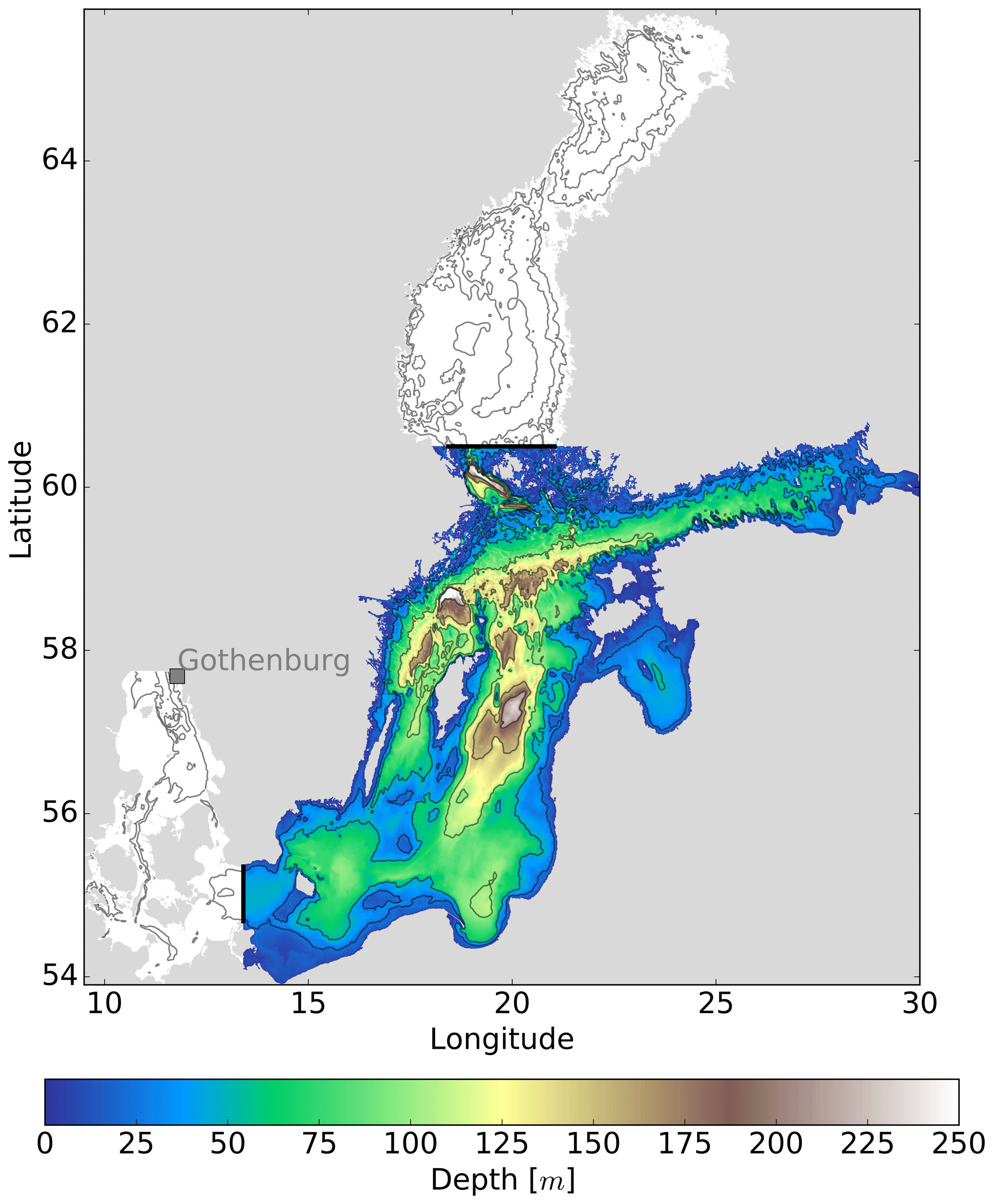
Figure 2Map of the high-resolution model domain (filled colors) with the open boundary locations (black lines). The coarse-resolution model domain (blank contours + filled colors) has an open boundary close to the Gothenburg station.
The model simulation run was performed from 1 April to 9 October 2015. The model domain had the western open boundary in the Arkona Basin and the northern open boundary at the entrance to the Bothnian Sea. For the open boundary conditions the one-way nesting approach was used and the results from the coarse-resolution model were utilized at the boundaries. Sea level fluctuations with 1-hourly resolution as well as temperature, salinity and current velocity profiles with 3-hourly resolution were interpolated using the nearest-neighbor method in space to the higher-resolution grid. In addition, the profiles were extended to the bottom of the high-resolution model. The coarse-resolution model covers the entire Baltic Sea with an open boundary in the Kattegat and has a horizontal resolution of 0.5 nautical miles (926 m) over the whole model domain. The coarse-resolution model run started from 1 April 2010 with initial thermohaline conditions taken from the Baltic Sea reanalysis for 1989–2015 by the Copernicus Marine Service. More detailed information on the coarse-resolution model is available in Zhurbas et al. (2018).
The atmospheric forcing (the wind stress and surface heat flux components) is calculated from the wind, solar radiation, air temperature, total cloudiness and relative humidity data generated by HIRLAM (High Resolution Limited Area Model) maintained operationally by the Estonian Weather Service with a spatial resolution of 11 km and temporal resolution of 1 h (Männik and Merilain, 2007). The wind velocity components at the 10 m level along with other HIRLAM meteorological parameters are interpolated to the model grid.
Freshwater input from the 54 largest Baltic Sea rivers together with their interannual variability is taken into account in the coarse-resolution model. The original dataset consists of daily climatological values of discharge for each river, but interannual variability is added by adjusting the freshwater input to different basins of the sea to match the values reported annually by HELCOM (Johansson, 2018).
The initial thermohaline field was obtained from the coarse-resolution model for 1 April 2015 and interpolated using the nearest-neighbor method to the high-resolution model grid. In addition, as the adaptive vertical coordinates were used in both setups, the T∕S profiles from coarse resolution were linearly interpolated to fixed 10 m vertical resolution before interpolation to the high resolution. The prognostic model runs were started from a motionless state and zero sea surface elevation. The spin-up time of the southern Baltic Sea model under the atmospheric forcing was expected to be within 10 d (Krauss and Brügge, 1991; Lips et al., 2016), while the model output for comparison with the respective satellite imagery was obtained after 45 d of simulation.
2.2 Application of synthetic floating particles approach to extract rotary characteristics of submesoscale cyclones and anticyclones
In order to characterize the submesoscale eddies, we estimated the eddy radius R, the dependence of the angular velocity of rotation ω(r) on the radial distance from the eddy center r, angular velocity in the eddy center ω0≡ω(0), differential rotation parameter and helicity parameter Hel, which will be defined later. The approach to calculate ω(r) and other parameters is illustrated in Fig. 3, where a pseudo-trajectory of a synthetic floating particle deployed within a modeled submesoscale eddy is presented. The pseudo-trajectory was calculated using a frozen velocity field; i.e., we took the modeled surface velocities for a given instant and kept the velocity field stationary during the whole advection period.
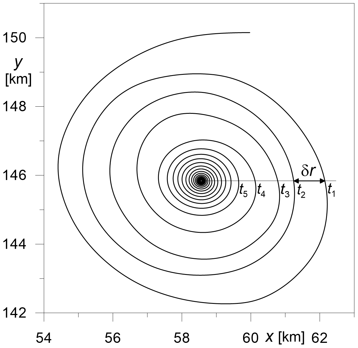
Figure 3An example pseudo-trajectory for a synthetic floating particle deployed in a submesoscale eddy. The pseudo-trajectory was calculated using a surface velocity field in the southeastern Baltic Sea simulated for the time moment 15 May 2015, 12:00 UTC (the frozen field approach). The particle was released in the periphery of the submesoscale cyclonic eddy c1 (see Fig. 4).
If t1 and t2 are the start and end time of a full particle loop (see Fig. 3), respectively, then the current values of ω and r can be calculated as
where l is the length of the pseudo-trajectory loop corresponding to the time interval [t1,t2]. Note that a plain linear relation between the vertical vorticity ζ and the frequency of rotation in the axisymmetric eddy, ζ=2ω is valid only for solid-body rotation when ω(r)=const, while for the differential rotation a more complicated formula is applied:
where Vφ is the transversal component of velocity.
The helicity parameter can be introduced as
where δr is the change in r, either positive or negative, for two consecutive loops with radii r1 and r2, respectively (see Fig. 3). In the case of the axisymmetric eddy the helicity parameter in Eq. (3) can be rewritten as , where Vr is the radial component of velocity, and in the case of no differential rotation–divergence in the axisymmetric eddy it can be expressed through the ratio of divergence and vorticity as . In view of continuity the vertical velocity W, which is responsible for upwelling–downwelling in the eddy, is determined near the surface by horizontal divergence D and depth z as W=zD. Deploying synthetic floating particles at different distances from the eddy center and applying the approach in Eqs. (1)–(3), one can build functions ω(r) and Hel(r). The modeled velocities were bilinearly interpolated to the current position of the particle within the grid cell. Therefore, if the initial position of the particle was taken close enough to the exact center of the eddy, the radius of the loop r would be sufficiently small, e.g., smaller than the grid cell size dx, dy=232 m. The frequency of a particle's rotary motion at m was taken for ω(0). If a particle is deployed at a large enough distance from the eddy center, the pseudo-trajectory will inevitably cease to be looped, and the largest r calculated from a still loop-shaped trajectory is taken for the eddy radius R. Once ω(r), Hel(r) and R are calculated, one can assess differential rotation Dif, the mean helicity parameter 〈Hel〉 and angular velocity in the eddy center ω0 as
According to Eq. (4) the differential rotation parameter was introduced as a relative change in the frequency of rotation between the eddy center and the periphery. Instead of ω0 we used the normalized frequency of rotation in the eddy center , where f is the Coriolis frequency. Note that Hel(r) is, in principle, an alternating function that proves the necessity of its averaging to get the bulk value 〈Hel〉. The positive–negative value of 〈Hel〉 manifests the divergence–convergence of currents and the related upwelling–downwelling in the surface layer of the eddy.
A large value of Dif and ω0 and the negative value of Hel(r) favor the formation of spirals in the tracer field from linear features. Indeed, if Dif=0 (solid-body rotation) the linear feature within the eddy will remain linear but rotated by some angle relative to the initial position (i.e., no spiral pattern is formed), whereas a positive 〈Hel〉 will result in sweeping the particles out from the eddy core, thus making the spiral less visible. And the large value of ω0 will accelerate the formation of the spiral in the tracer field provided that Dif is large enough and 〈Hel〉 is negative (or sufficiently small positive). Since the spirals are known to be overwhelmingly cyclonic, one may expect that Dif and ω0 will be larger and 〈Hel〉 will be smaller for the submesoscale cyclonic eddies relative to those for the anticyclonic eddies.
Apart from the above-defined rotary characteristics of submesoscale eddies calculated from frozen velocity field, we utilized some numerical experiments with the deployment of synthetic floating particles in the modeled nonstationary (not frozen) velocity field, namely when the particles were uniformly seeded on the sea surface and when the particles were seeded on a line passed through the center of a cyclonic or anticyclonic eddy.
The trajectories of synthetic floating particles were calculated using simulated current velocity in the uppermost model cell with 10 min temporal resolution by means of the numerical integration of plain equations for Lagrangian particle advection with a Runge–Kutta scheme of higher-order of accuracy (Väli et al., 2018).
3.1 Modeled submesoscale fields of surface velocity and temperature in comparison with satellite imagery
Modeled snapshots of surface layer temperature, salinity and currents with submesoscale resolution in the southeastern Baltic Sea for 15 May, 8 June and 3 July 2015 are shown in Figs. 4–6, respectively. These snapshots were chosen because they corresponded to three days at the beginning of the modeling period for which there were satellite images available (one of the images is presented in Fig. 1). The snapshots demonstrate a quite dense packing of the sea surface with submesoscale eddies. Similar dense packing of the sea surface with submesoscale eddies was observed in Envisat ASAR WSM images of the southeastern Baltic Sea (Karimova et al., 2012). Looking at the snapshots of the surface layer currents (Figs. 4c–6c), one cannot see any predominance of the number of cyclones over the number of anticyclones or vice versa. However, the surface layer temperature and salinity snapshots (panels a and b, respectively) clearly demonstrate a large number of spiral structures linked with the submesoscale cyclonic eddies, while the submesoscale anticyclones, as a rule, do not manifest themselves by well-defined spirals.
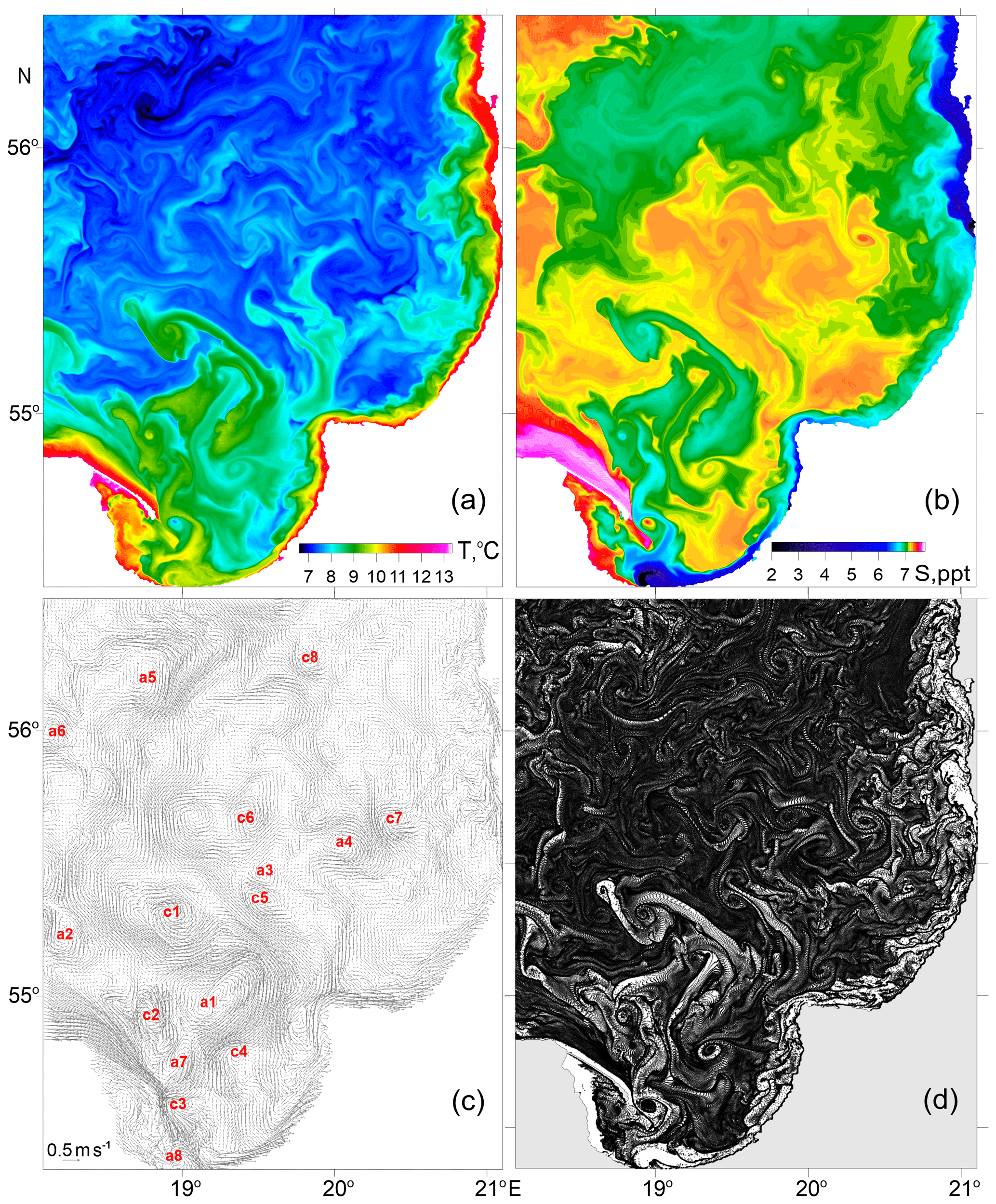
Figure 4Modeled fields of the surface layer parameters in the southeastern Baltic Sea on 15 May 2015, 12:00 UTC: temperature (a), salinity (b), current velocity (c) and spatial distribution of uniformly released synthetic floating Lagrangian particles (d) after 1 d of advection. The red labels in panel (c) point at the cyclonic (c1, c2, etc.) and anticyclonic (a1, a2, etc.) eddies used to calculate the rotary characteristics in Sect. 3.4 (see Table 1).
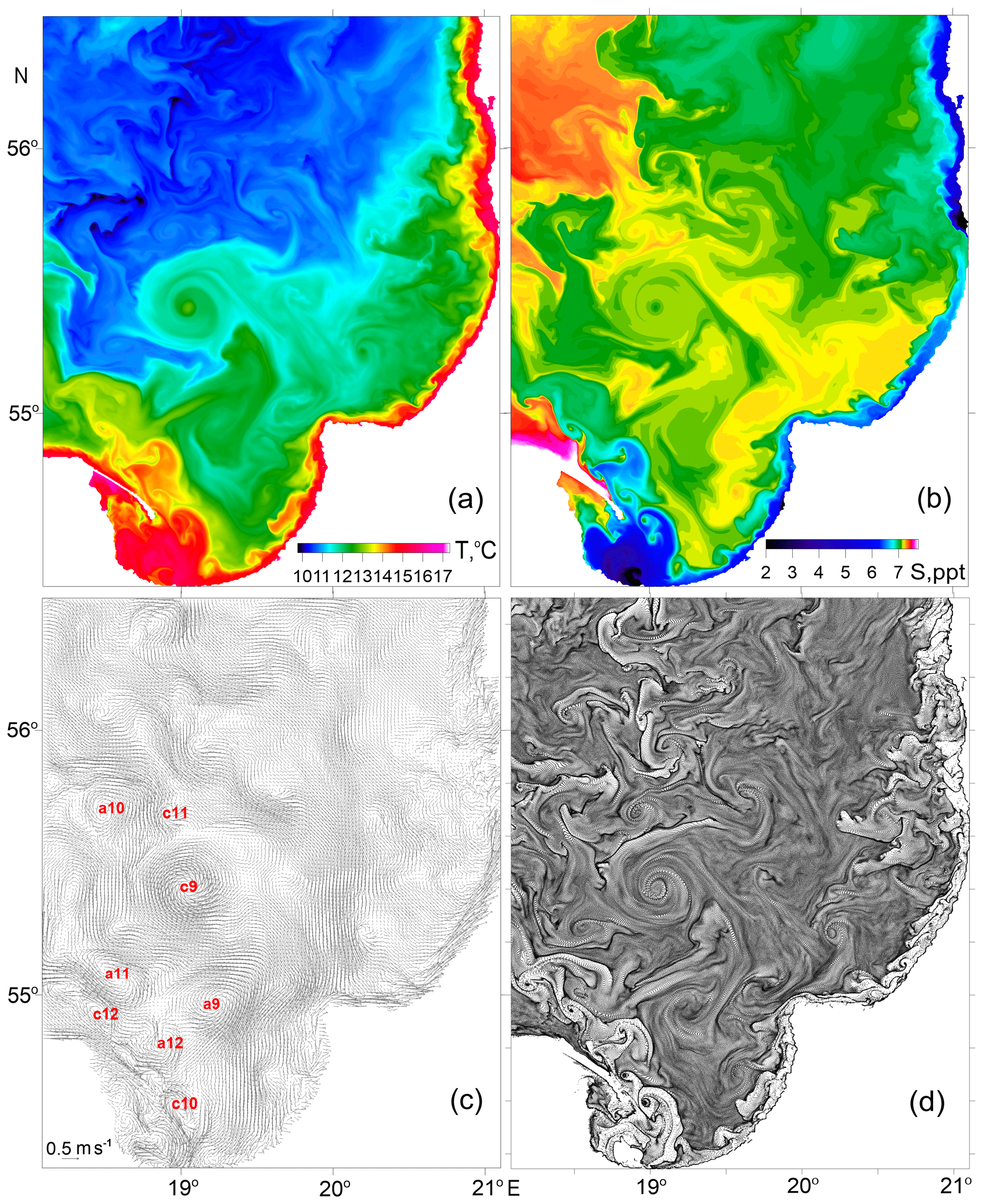
Figure 5The same as in Fig. 4 but for 8 June 2015, 12:00 UTC.
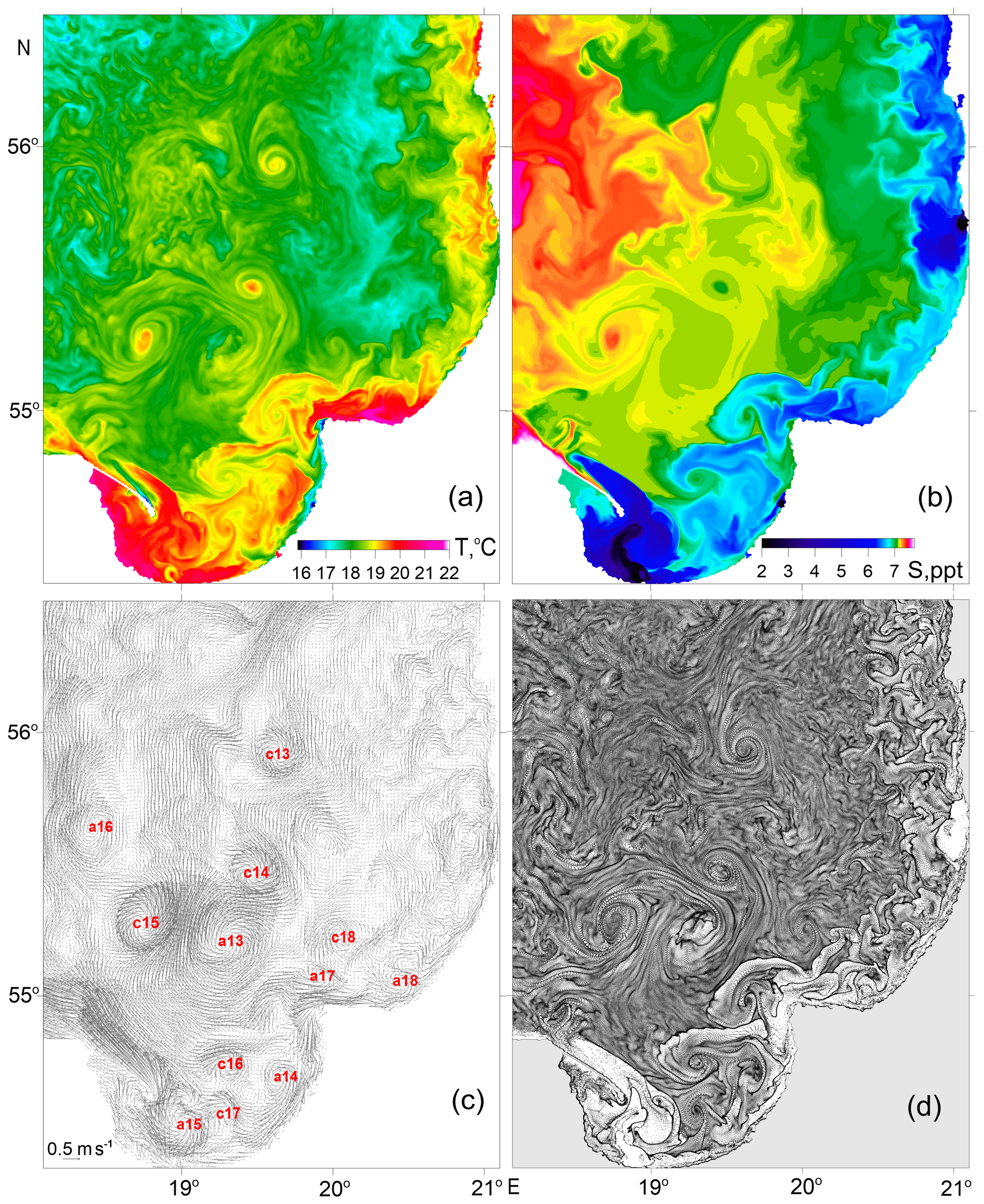
Figure 6The same as in Figs. 4 and 5 but for 3 July 2015, 12:00 UTC.
Despite the fact that salinity is believed to be a more conservative tracer than temperature, the spirals in the temperature field seem more pronounced than those in the salinity field (see Figs. 4a, b–6a, b). Probably, the reason lies in the fact that the mixed layer under conditions of the seasonal thermocline is characterized by small but noticeable vertical temperature gradients and vanishingly small vertical salinity gradients. Following Branningan (2016), it can be assumed that the spirals in the surface temperature field are associated with the alternation of upwelling–downwelling cells with a transverse wavelength of the order of 1 km in the mixed layer of a differentially rotating eddy, caused by submesoscale instabilities.
Some of the simulated submesoscale eddies shown in Figs. 4–6 were chosen for further calculations of their rotary characteristics by means of the approach described in Sect. 2.2. In total, the calculations were performed for 18 anticyclonic and 18 cyclonic eddies marked in Figs. 4c–6c as a1–a18 and c1–c18, respectively. The eddies were chosen by hand as the most prominent vortices seen in Figs. 4–6. The number of vortices to be processed (18 cyclones and 18 anticyclones) was selected as a compromise between the requirement to provide statistically significant results and the time spent on obtaining a suitable sample of eddies. Note that the procedure for calculating the rotary characteristics of the eddy described in Sect. 2.2 was not fully automated and was therefore quite time-consuming. The results are presented in Sect. 3.4.
Note that the modeled snapshots of surface layer temperature and currents presented in Fig. 6 correspond to the date 3 July 2015, for which we have a true color image of the southeastern Baltic Sea from Landsat-8 (Fig. 1). A vortex pair seen in the satellite image at a distance of 30–60 km northwest from Cape Taran can also be identified in the simulated temperature and current fields of the surface layer; it is labeled as c14 and a13 in Fig. 6c. Moreover, to the south of the vortex pair c14–a13 in the Gulf of Gdańsk, both the model and the satellite image display two to three cyclonic eddies (cf. Figs. 1 and 6). The fact that a vortex pair of almost the same size and orientation was modeled in almost the same place and at the same time as the observed vortex pair can be considered a validation of the model.
3.2 Numerical experiments with spatially uniform release of synthetic floating particles
Patterns formed on the sea surface by synthetic floating Lagrangian particles were shown to be a powerful tool to visualize mesoscale–submesoscale structures (Väli et al., 2018). Examples of such patterns are also presented in Figs. 4d–6d. The particles were seeded uniformly (i.e., one particle in the center of every grid bin; the total number of particles was approx. 1 million) within the model domain a day before the date specified in Figs. 4–6 and carried by the simulated nonstationary currents during 1 d (i.e., τ=1 d, where τ is the advection time). Soon after the release of synthetic floating particles, the horizontally uniform distribution of particles was transformed into a pattern that resembles the corresponding maps of oceanographic tracers such as temperature and/or salinity in the surface layer. Note that within just 1 d of advection the uniformly distributed particles clustered predominantly into cyclonic spirals corresponding to submesoscale eddies.
3.3 Numerical experiments with linearly aligned release of synthetic floating particles in submesoscale cyclones and anticyclones
Keeping in mind that according to Munk et al. (2000) the spirals can be formed from linear surface features wound by vortices, numerical experiments were performed with synthetic floating particles initially clustered in zonally aligned features intersecting the centers of the submesoscale cyclones marked as c13–c18 and anticyclones marked as a13–a16 and a18 in Fig. 6. Figure 7 shows the evolution of a linear feature of a large number of synthetic floating particles in 1 and 2 d of advection in the simulated velocity field. Note that the anticyclone a17 was omitted because this eddy appeared to be too young: it could not be clearly identified 2 d before 3 July 2015 to seed synthetic particles on a line passed through its center. It is clearly seen from Fig. 7 that the spirals were formed only from the linear features embedded into the submesoscale cyclonic eddies, while the linear features in the anticyclonic eddies transformed to some curves of irregular shape.
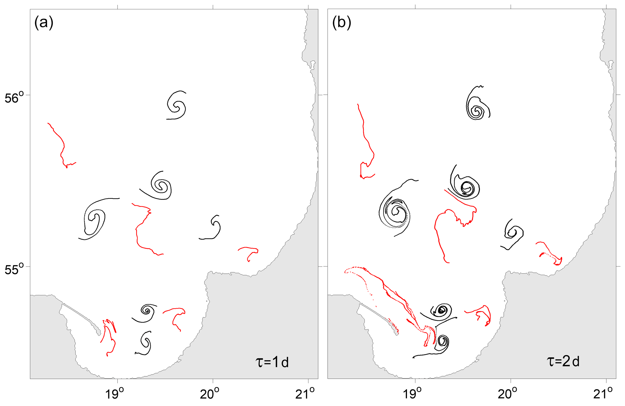
Figure 7Patterns formed on 3 July 2015 from zonally elongated linear features passing through the centers of the simulated submesoscale cyclonic (black curves) and anticyclonic (red curves) eddies after (a) 1 d and (b) 2 d of advection. The linear features included a large number (2000) of synthetic floating particles deployed 1 d (a) and 2 d (b) before 3 July 2015, 12:00 UTC.
3.4 Numerical experiments with the release of synthetic floating particles in a frozen velocity field to extract rotary characteristics of submesoscale cyclones and anticyclones
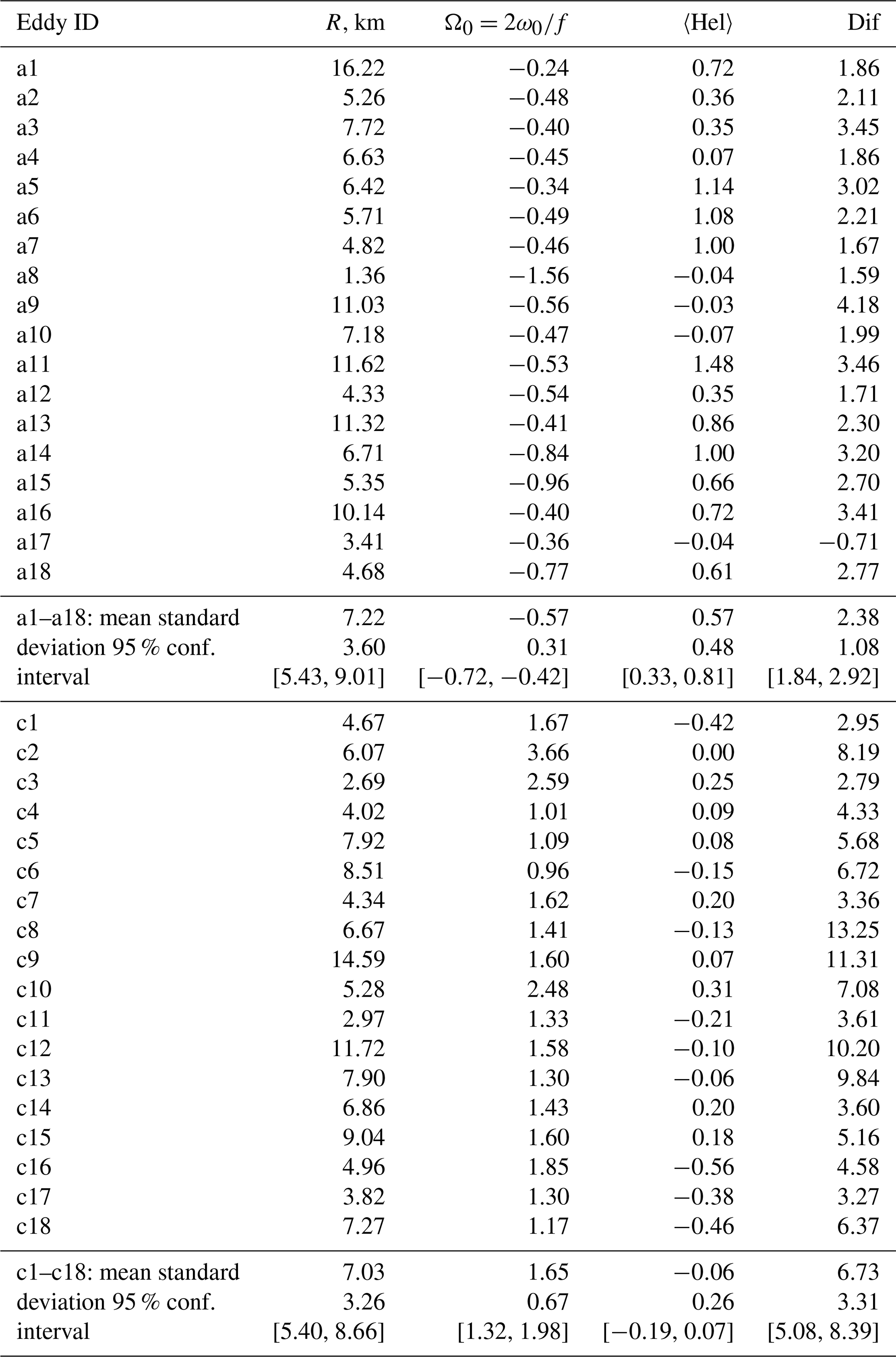
Applying the approach described in Sect. 2.2, the rotary characteristics R, , Dif and 〈Hel〉 were calculated for 18 anticyclonic eddies and 18 cyclonic eddies (marked as a1–a18 and c1–c18, respectively, in Figs. 4c–6c). The rotary characteristics of individual eddies along with the mean values, standard deviations and 95 % confidence intervals calculated for the anticyclones and cyclones separately are presented in Table 1 (see Appendix A). For clarity, the scatter plots of R, Dif and 〈Hel〉 vs. Ω0 are shown in Fig. 8.
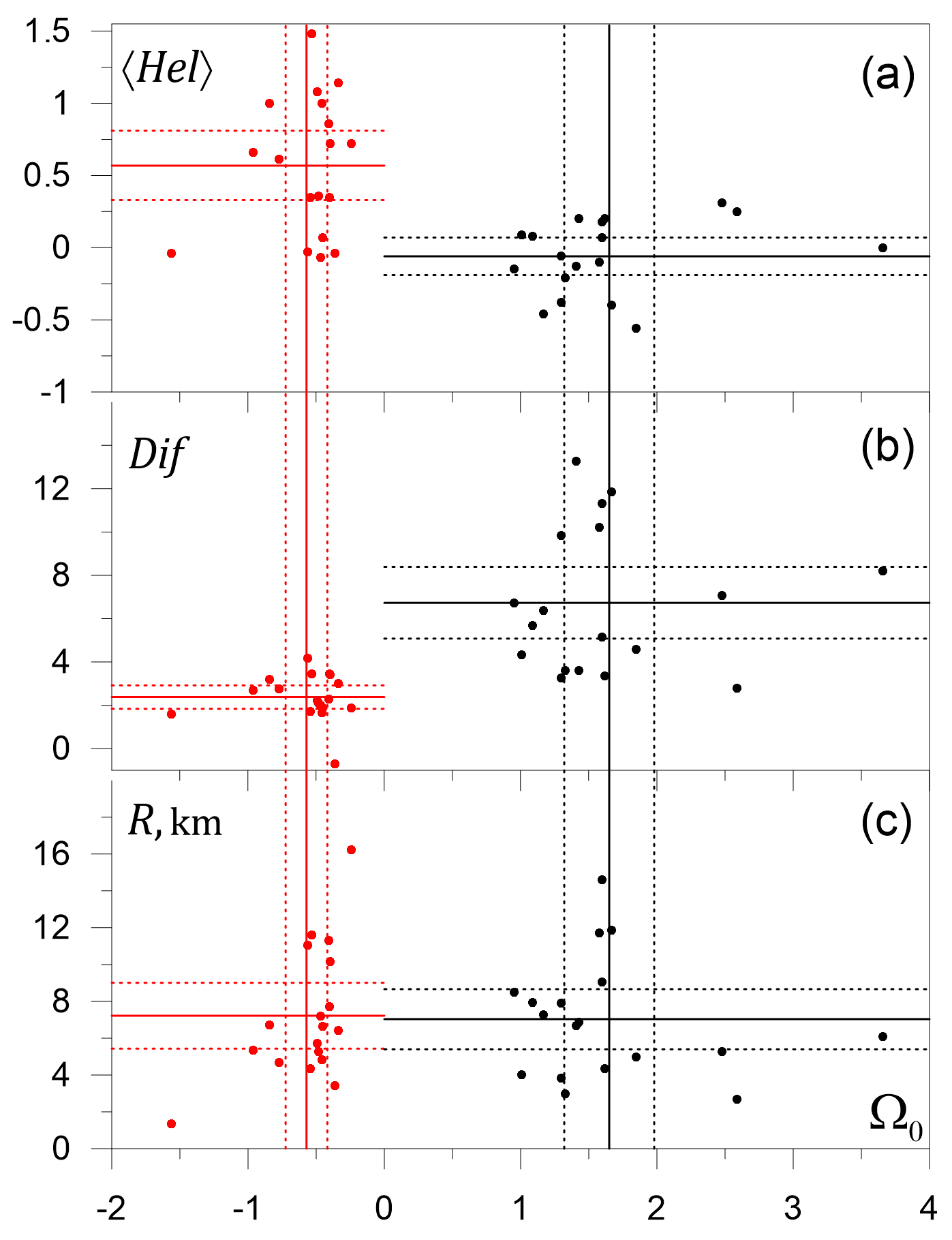
Figure 8Scatter plots of the helicity (a), differential rotation (b) parameters and radius (c) of a submesoscale eddy vs. the normalized frequency of rotation in the eddy center. Horizontal and vertical lines are the mean values (solid) and 95 % confidence limits (dotted) of the parameters calculated separately for the anticyclonic (Ω0<0, red lines and symbols) and cyclonic (Ω0>0, black lines and symbols) eddies based on the Student's t distribution.
The statistics of the submesoscale eddy size R are almost the same for anticyclones and cyclones, with mean values of 7.22 and 7.03 km, respectively. In contrast to the eddy size R, the rotary characteristics of submesoscale cyclones, such as Ω0, Dif and 〈Hel〉, differ considerably from the respective values of the anticyclones. Namely, the mean value of Ω0 is 1.65 for cyclones and −0.57 for anticyclones; i.e., the absolute frequency of rotation in the center of the cyclonic eddy is on average 3 times larger than in the anticyclone. It is also important that the cyclonic eddies are characterized by much more pronounced differential rotation (the mean value of Dif is 6.73 in the cyclones vs. 2.38 in the anticyclones). Lastly, there is a substantial difference in the helicity: the rotary motion of a particle around the center of the submesoscale cyclonic eddy is accompanied on average by a shift towards the eddy center (the mean value of 〈Hel〉 is negative at −0.06), while in an anticyclone a particle moves on average away from the center (the mean value of 〈Hel〉 is positive at 0.57). It is worth noting that the 95 % confidence intervals for the mean values of Dif and 〈Hel〉 of the cyclonic eddies do not overlap those of the anticyclonic eddies.
Finally, Fig. 9 presents plots of the normalized frequency of rotation ω∕ω0 vs. the radial distance from the eddy center r∕R of the modeled submesoscale cyclonic (a) and anticyclonic (b) eddies. The ensemble mean curve of for cyclones displays a much larger drop in the rotation frequency away from the eddy center (i.e., more pronounced differential rotation) and the positive curvature (the second derivative F′′ is positive). In contrast, the ensemble mean curve of for anticyclones displays a much smaller drop in the rotation frequency away from the eddy center (i.e., less pronounced differential rotation) and the negative curvature (the second derivative F′′ is negative).

Figure 9Normalized dependence of the angular velocity of rotation ω∕ω0 on the radial distance from the eddy center r∕R in the simulated submesoscale eddies: cyclones c1–c18 (a) and anticyclones a1–a18 (b) (thin dashed curves). The bold solid and bold dotted curves are the ensemble means and the 95 % confidence intervals, respectively. The black and red curves correspond to the cyclonic and anticyclonic eddies.
As stated in the Introduction, this work aimed to investigate the differences between the rotary characteristics of submesoscale cyclonic and anticyclonic eddies, which, in our opinion, would explain the overwhelming dominance of cyclonic spirals on satellite images of the sea surface recorded in the SAR, infrared and optical ranges. In this study we used numerical experiments with floating Lagrangian particles embedded offline in a regional circulation model of the southeastern Baltic Sea with very high horizontal resolution (0.125 nautical mile grid).
The numerical experiments showed that cyclonic spirals can be formed from both a horizontally uniform initial distribution of floating particles and from initially lined-up particle clusters during an advection time of the order of 1 d. While the formation of predominantly cyclonic spirals in the tracer field from linear features in the course of the development of horizontal shear instabilities and mixed-layer baroclinic instabilities is a well-known effect that was thoroughly discussed by Munk et al. (2000) and Eldevik and Dysthe (2002), a quick regrouping of the floating particles from a horizontally uniform distribution to cyclonic spirals in the course of advection in the submesoscale velocity field is a surprising phenomenon, which was first mentioned by Väli et al. (2018).
We addressed several rotary characteristics of submesoscale eddies that could potentially be responsible for the predominant formation of cyclonic spirals in the tracer field, such as the following:
-
normalized frequency of rotation in the eddy center (the higher the frequency, the faster the spiral can be formed);
-
the differential rotation parameter (the spirals cannot be formed from linear features at the solid-body rotation when Dif=0); and
-
the helicity parameter 〈Hel〉 defined in Sect. 2.2 (if 〈Hel〉<0 the particles shift towards the eddy center, which makes the spiral more visible, and, in contrast, if 〈Hel〉>0 the particles shift away from the eddy center, which makes the spiral less visible).
To calculate Ω0, Dif, 〈Hel〉 and the eddy radius R the approach described in Sect. 2.2 was applied to the pseudo-trajectories of synthetic floating particles in a frozen velocity field (i.e., the velocity field simulated by the circulation model for a given instant was kept stationary for the entire period of advection). As a result, we obtained estimates of Ω0, Dif, 〈Hel〉 and R for 18 cyclonic and 18 anticyclonic submesoscale eddies simulated in the southeastern Baltic Sea in May–July 2015.
The ensemble mean value of the eddy radius R was 7.22 and 7.03 km for the anticyclones and cyclones, respectively, with strong overlap of the 95 % confidence intervals. Therefore, one may conclude that submesoscale cyclonic eddies are indistinguishable by size from submesoscale anticyclonic eddies.
In contrast to R, the ensemble mean values of Ω0, Dif and 〈Hel〉 were substantially different for the cyclonic and anticyclonic eddies, and the difference of all three rotary characteristics indicated the predominant formation of cyclonic spirals in the tracer field. Indeed, the ensemble mean values of Ω0, Dif and 〈Hel〉 were 1.65 vs. −0.57, 6.73 vs. 2.38 and −0.06 vs. 0.57 for cyclones and anticyclones, respectively, and the 95 % confidence intervals did not overlap (see Table 1 and Fig. 8). Therefore, on average the submesoscale cyclonic eddies, in comparison to the anticyclonic ones, rotate 3 times faster, have a 3 times larger difference in the frequency of rotation between the eddy center and the periphery, and display the tendency of shifting floating particles towards the eddy center (〈Hel〉<0). Note that the negative–positive value of the helicity parameter 〈Hel〉 in the cyclonic–anticyclonic eddies is in accordance with the negative correlation between relative vorticity and vertical velocity in the submesoscales reported by Väli et al. (2017) (i.e., submesoscale cyclonic–anticyclonic eddies are characterized mostly by downwelling–upwelling).
The physical intuition for the faster spinning of cyclonic eddies vs. anticyclonic eddies can be gained from the conservation of potential vorticity in a fluid parcel (e.g., Väli et al., 2017): , where ρz is the vertical gradient of density. If the parcel undergoes ultimate vertical stretching (, where ρz(0) is the initial value of ρz) given that it does not spin initially (ζ(0)=0), it will acquire unlimited cyclonic rotation: . In contrast, if the parcel undergoes ultimate vertical squeezing (), it will acquire anticyclonic rotation limited from above: . The above considerations make it clear why in Fig. 8 in all cyclonic eddies Ω0>1, while in all anticyclonic eddies except one the rotation speed is within . As for the positive–negative value of helicity in anticyclonic–cyclonic eddy, it can be intuitively understood by taking into account that the related upwelling–downwelling implies potential energy loss and therefore relaxation of the eddy.
The frequency of rotation of submesoscale eddies was found to decrease with the radial distance (i.e., the rotation is differential rather than solid body). However, a certain similarity of solid-body rotation is still inherent in the submesoscale anticyclones, wherein the difference in the frequency of rotation between the eddy center and periphery is relatively small, and the second derivative of frequency with respect to radial distance is negative (see Fig. 9b). In contrast to the submesoscale anticyclones, in the submesoscale cyclones, wherein the difference in the frequency of rotation between the center and the periphery is much larger and the second derivative of frequency with respect to radial distance is positive, one cannot see even a hint of solid-body rotation (cf. Fig. 9a and b).
We realize that the scenario presented in Sect. 3.3, in which the spiral in the tracer field is formed from synthetic floating particles seeded on a line passed through the center of a mature submesoscale cyclonic or anticyclonic eddy, is barely realistic because one can hardly imagine a natural phenomenon capable of providing such seeding. However, the two other scenarios, i.e., when the spirals come from the advection of uniformly seeded floating particles into the velocity field of a mature eddy (see Sect. 3.2) and from the reshaping of a linear tracer feature aligned to the density front in the course of the development of a kind of frontal instability (the Munk's hypothesis), seem quite realistic. In our opinion, depending on the specific conditions of the ocean environment, either the first or second of the two realistic scenarios may prevail.
Statistical processing of the trajectories of the synthetic floating particles allowed us to conclude that the submesoscale cyclonic eddies differ from the anticyclonic eddies in three ways favoring the formation of spirals in the tracer field: they can be characterized by (a) a considerably higher angular velocity, (b) a more pronounced differential rotation and (c) a negative helicity. The differences in the rotary characteristics of submesoscale cyclonic and anticyclonic eddies were statistically assessed from a limited model output for early summer 2015 in the southeast Baltic Sea, and we could not exclude the seasonal and interannual variability of the studied parameters or some dependences on the eddy age and life span. These issues could be the subject of future research.
The IOW branch of the GETM code is publicly accessible from https://gitlab.io-warnemuende.de/getm/code.git (last access: 30 November 2019; Burchard and Bolding, 2002), GOTM from https://gitlab.io-warnemuende.de/gotm/code.git (last access: 30 November 2019; Burchard and Bolding, 2001) and FABM from https://github.com/fabm-model/fabm.git (last access: 30 November 2019; Bruggeman and Bolding, 2014).
The Copernicus Marine Service reanalysis and historical tide gauge observations can be accessed from their web page at http://marine.copernicus.eu/services-portfolio/access-to-products/ (last access: 30 November 2019; CMEMS, 2019). The HIRLAM atmospheric forcing was available courtesy of the Estonian Weather Service. The model simulation data can be obtained from the authors upon request.
Table A1Rotary characteristics of submesoscale cyclonic and anticyclonic eddies.
VZ designed and performed numerical experiments with floating Lagrangian particles and prepared the paper with contributions from all coauthors. GV performed submesoscale circulation modeling. NK provided a physical interpretation of the numerical experiments with floating Lagrangian particles.
The authors declare that they have no conflict of interest.
The allocation of computing time on the high-performance computing cluster by the Tallinn University of Technology and by the University of Tartu is gratefully acknowledged. Germo Väli (submesoscale circulation modeling) was supported by institutional research funding IUT 19-6 from the Estonian Ministry of Education and Research and BONUS, the joint Baltic Sea research and development program (Art 185) funded jointly by the European Union's Seventh Programme for research, technological development and demonstration, and by the Estonian Research Council through grant VEU17107 (BONUS INTEGRAL). Victor Zhurbas and Natalia Kuzmina (designing, performing and interpreting the numerical experiments with floating Lagrangian particles) were supported by budgetary financing from the Shirshov Institute of Oceanology RAS (project no. 149-2019-0003). The authors are grateful to four reviewers for their kind attitude and comprehensive reviews.
This research has been supported by the Russian Foundation for Basic Research (grant no. 18-05-80031), institutional research funding from the Estonian Ministry of Education and Research (grant no. IUT 19-6), the joint Baltic Sea research and development program (Art 185) funded jointly by the European Union's Seventh Programme for research, technological development and demonstration, the Estonian Research Council (BONUS INTEGRAL (grant no. VEU17107)), and budgetary financing from the Shirshov Institute of Oceanology RAS (grant no. 149-2019-0003).
This paper was edited by Eric J. M. Delhez and reviewed by Vladimir Ryabchenko and three anonymous referees.
Barkan, R., McWilliams, J. C., Shchepetkin, A. F., Molemaker, M. J., Renault, L., Bracco, A., and Choi, J.: Submesoscale dynamics in the northern Gulf of Mexico. Part I: Regional and seasonal characterization and the role of river outflow, J. Phys. Oceanogr., 47, 2325–2346, https://doi.org/10.1175/JPO-D-17-0035.1, 2017.
Boccaletti, G., Ferrari, R., and Fox-Kemper, B.: Mixed layer instabilities and restratification, J. Phys. Oceanogr., 37, 2228–2250, https://doi.org/10.1175/JPO3101.1, 2007.
Brannigan, L.: Intense submesoscale upwelling in anticyclonic eddies, Geophys. Res. Lett., 43, 3360–3369, https://doi.org/10.1002/2016GL067926, 2016.
Brannigan, L., Marshall, D. P., Naveira-Gabarato, A. C., Nurser, A. J. G., and Kaiser, J.: Submesoscale Instabilities in Mesoscale Eddies, J. Phys. Oceanogr., 47, 3061–3085, https://doi.org/10.1175/JPO-D-16-0178.1, 2017.
Bruggeman, J. and Bolding, K.: A general framework for aquatic biogeochemical models, Environ. Modell. Softw., 61, 249–265, https://doi.org/10.1016/j.envsoft.2014.04.002, 2014.
Buckingham, C. E., Khaleel, Z., Lazar, A., Martin, A. P., Allen, J. T., Garabato, A. C. N., Thompson, A. F., and Vic, C.: Testing Munk's hypothesis for submesoscale eddy generation using observations in the North Atlantic, J. Geophys. Res.-Oceans, 122, 6725–6745, https://doi.org/10.1002/2017JC012910, 2017.
Burchard, H. and Bolding, K.: Comparative Analysis of Four Second-Moment Turbulence Closure Models for the Oceanic Mixed Layer, J. Phys. Oceanogr., 31, 1943–1968, https://doi.org/10.1175/1520-0485(2001)031<1943:CAOFSM>2.0.CO;2, 2001.
Burchard, H. and Bolding, K.: GETM – a general estuarine transport model, Scientific documentation, Technical report EUR 20253 EN, European Commission, Ispra, Italy, available at: https://op.europa.eu/en/publication-detail/-/publication/5506bf19-e076-4d4b-8648-dedd06efbb38 (last access: 3 December 2019), 2002.
Canuto, V. M., Howard, A., Cheng, Y., and Dubovikov, M. S.: Ocean Turbulence. Part I: One-Point Closure Model–Momentum and Heat Vertical Diffusivities, J. Phys. Oceanogr., 31, 1413–1426, https://doi.org/10.1175/1520-0485(2001)031<1413:OTPIOP>2.0.CO;2, 2001.
Capet, X., McWilliams, J. C., Molemaker, M. J., and Shchepetkin, A. F.: Mesoscale to submesoscale transition in the California Current system, Part I: flow structure, eddy flux, and observational tests, J. Phys. Oceanogr., 38, 29–43, https://doi.org/10.1175/2007JPO3671.1, 2008.
CMEMS: The Copernicus Marine Service re-analysis for Baltic Sea – product BALTICSEA_REANALYSIS_PHY_003_011, created by: Swedish Meteorological and Hydrological Institute (SMHI) and tide-gauge observations – product INSITU_BAL_NRT_OBSERVATIONS_013_032, created by: BSH, Germany, SMHI, Sweden, FMI, Finland, and DMI, Denmark, available at: http://marine.copernicus.eu/services-portfolio/access-to-products/, last access: 30 November 2019.
D'Asaro, E. A., Shcherbina, A. Y., Klymak, J. M., Molemaker, J., Novelli, G.,Guigand, C. M., Haza, A. C., Haus, B. K., Ryan, E. H., Jacobs, G. A., Huntley, H. S., Laxague, N. J. M., Chen, S., Judt, F., McWilliams, J. C., Barkan, R., Kirwan Jr., A. D., Poje, A. C., and Özgökmen, T. M.: Ocean convergence and the dispersion of flotsam, P. Natl. Acad. Sci. USA, 115, 1162–1167, https://doi.org/10.1073/pnas.1802701115, 2018.
Dewar, W. K., McWilliams, J. C., and Molemaker, M. J.: Centrifugal instability and mixing in the California Undercurrent, J. Phys. Oceanogr., 45, 1224–1241, https://doi.org/10.1175/JPO-D-13-0269.1, 2015.
Eldevik, T. and Dysthe K. B.: Spiral eddies, J. Phys. Oceanogr., 32, 851–869, https://doi.org/10.1175/1520-0485(2002)032h0851:SEi2.0.CO;2, 2002.
Fox-Kemper, B., Ferrari, R., and Hallberg, R.: Parameterization of mixed layer eddies. Part I: Theory and diagnosis, J. Phys. Oceanogr., 38, 1145–1165, https://doi.org/10.1175/2007JPO3792.1, 2008.
Fox-Kemper, B., Danabasoglu, G., Ferrari, R., Griffies, S., Hallberg, R., Holland, M., Maltrud, M., Peacock, S., and Samuels, B.: Parameterization of mixed layer eddies. III: Implementation and impact in global ocean climate simulations, Ocean Model., 39, 61–78, https://doi.org/10.1016/j.ocemod.2010.09.002, 2011.
Ginzburg, A. I., Krek, E. V., Kostianoy, A. G., and Solovyev, D. M.: Evolution of mesoscale anticyclonic vortex and vortex dipoles/multipoles on its base in the south-eastern Baltic (satellite information May–July 2015), Okeanologicheskie issledovaniya (Journal of Oceanological Research), 45, 10–22, https://doi.org/10.29006/1564-2291.JOR-2017.45(1).3, 2017 (in Russian).
Gräwe, U., Holtermann, P., Klingbeil, K., and Burchard, H.: Advantages of vertically adaptive coordinates in numerical models of stratified shelf seas, Ocean Model., 92, 56–68, https://doi.org/10.1016/j.ocemod.2015.05.008, 2015.
Gula, J., Molemaker, M. J., and McWilliams, J. C.: Submesoscale dynamics of a Gulf Stream frontal eddy in the South Atlantic Bight, J. Phys. Oceanogr., 46, 305–325, https://doi.org/10.1175/JPO-D-14-0258.1, 2016.
Haine, T. W. and Marshall, J.: Gravitational, symmetric, and baroclinic instability of the ocean mixed layer, J. Phys. Oceanogr., 28, 634–658, https://doi.org/10.1175/1520-0485(1998)028<0634:GSABIO>2.0.CO;2, 1998.
Hofmeister, R., Burchard, H., and Beckers, J.-M.: Non-uniform adaptive vertical grids for 3D numerical ocean models, Ocean Model., 33, 70–86, https://doi.org/10.1016/j.ocemod.2009.12.003, 2010.
Johansson, J.: Total and regional runoff to the Baltic Sea, HELCOM Baltic Sea Environment Fact Sheets, available at: http://www.helcom.fi/baltic-sea-trends/environment-fact-sheets/, last access: 20 December 2018.
Kalda, J., Soomere, T., and Giudici, A.: On the finite-time compressibility of the surface currents in the Gulf of Finland, the Baltic Sea, J. Marine Syst., 129, 56–65, https://doi.org/10.1016/j.jmarsys.2012.08.010, 2014.
Karimova, S. S., Lavrova, O. Y., and Solov'ev, D. M.: Observation of Eddy Structures in the Baltic Sea with the Use of Radiolocation and Radiometric Satellite Data, Izv. Atmos. Ocean. Phy., 48, 1006–1013, https://doi.org/10.1134/S0001433812090071, 2012.
Krauss, W. and Brügge, B.: Wind-produced water exchange between the deep basins of the Baltic Sea, J. Phys. Oceanogr., 21, 373–384, https://doi.org/10.1175/1520-0485(1991)021<0373:WPWEBT>2.0.CO;2, 1991.
Laanemets, J., Väli, G., Zhurbas, V., Elken, J., Lips, I., and Lips, U.: Simulation of mesoscale structures and nutrient transport during summer upwelling events in the Gulf of Finland in 2006, Boreal Environ. Res., 16, 15–26, 2011.
Lips, U., Zhurbas, V., Skudra, M., and Väli, G.: A numerical study of circulation in the Gulf of Riga, Baltic Sea. Part I: Whole-basin gyres and mean currents, Cont. Shelf Res., 112, 1–13, https://doi.org/10.1016/j.csr.2015.11.008, 2016.
Männik, A. and Merilain, M.: Verification of different precipitation forecasts during extended winter-season in Estonia, HIRLAM Newsletter, 52, 65–70, 2007.
McWilliams, J. C.: Submesoscale currents in the ocean, P. Roy. Soc. A-Math. Phy., 72, 20160117, https://doi.org/10.1098/rspa.2016.0117, 2016.
Molemaker, M. J., McWilliams, J. C., and Dewar, W. K.: Submesoscale instability and generation of mesoscale anticyclones near a separation of the California Undercurrent, J. Phys. Oceanogr., 45, 613–629, https://doi.org/10.1175/JPO-D-13-0225.1, 2015.
Munk, W.: Spirals on the sea, Sci. Mar., 65, 193–198, https://doi.org/10.3989/scimar.2001.65s2193, 2001.
Munk, W., Armi, L., Fischer, K., and Zachariasen, F.: Spirals on the sea, P. Roy. Soc. A-Math. Phy., 456, 1217–1280, 2000.
Onken, R., Baschek, B., and Angel-Benavides, I. M.: Very high-resolution modelling of submesoscale turbulent patterns and processes in the Baltic Sea, Ocean Sci. Discuss., https://doi.org/10.5194/os-2019-44, in review, 2019.
Reichwaldt, E. S., Song, H., and Ghadouani, A.: Effects of the Distribution of a Toxic Microcystis Bloom on the Small Scale Patchiness of Zooplankton, PLoS ONE, 8, e66674, https://doi.org/10.1371/journal.pone.0066674, 2013.
Samuelsen, A., Hjøllo, S. S., Johannessen, J. A., and Patel, R.: Particle aggregation at the edges of anticyclonic eddies and implications for distribution of biomass, Ocean Sci., 8, 389–400, https://doi.org/10.5194/os-8-389-2012, 2012.
Thomas, L. N., Tandon, A., and Mahadevan, A.: Submesoscale processes and dynamics, in: Ocean Modeling in an Eddying Regime, edited by: Hecht, M. W. and Hasumi, H., American Geophysical Union, Washington, Geophysical Monograph Series, 177, 17–38, https://doi.org/10.1029/177GM04, 2008.
Thomas, L. N., Taylor, J. R., Ferrari, R., and Joyce, T. M.: Symmetric instability in the Gulf Stream, Deep-Sea Res. Pt. II, 91, 96–110, https://doi.org/10.1016/j.dsr2.2013.02.025, 2013.
Umlauf, L. and Burchard, H.: Second-order turbulence closure models for geophysical boundary layers. A review of recent work, Cont. Shelf Res., 25, 795–827, https://doi.org/10.1016/j.csr.2004.08.004, 2005.
Väli, G., Zhurbas, V., Lips, U., and Laanemets, J.: Submesoscale structures related to upwelling events in the Gulf of Finland, Baltic Sea (numerical experiments), J. Marine Syst., 171, 31–42, https://doi.org/10.1016/j.jmarsys.2016.06.010, 2017.
Väli, G., Zhurbas, V. M., Laanemets, J., and Lips, U.: Clustering of floating particles due to submesoscale dynamics: a simulation study for the Gulf of Finland, Fundamentalnaya i prikladnaya gidrofizika, 11, 21–35, https://doi.org/10.7868/S2073667318020028, 2018.
Vankevich, R. E., Sofina, E. V., Eremina, T. E., Ryabchenko, V. A., Molchanov, M. S., and Isaev, A. V.: Effects of lateral processes on the seasonal water stratification of the Gulf of Finland: 3-D NEMO-based model study, Ocean Sci., 12, 987–1001, https://doi.org/10.5194/os-12-987-2016, 2016.
Vortmeyer-Kley, R., Holtermann, P. L., Feudel, U., and Gräwe, U.: Comparing Eulerian and Lagrangian eddy census for a tide-less, semi-enclosed basin, the Baltic Sea, Ocean Dynam., 69, 701–717, https://doi.org/10.1007/s10236-019-01269-z, 2019.
Zhurbas, V. M., Stipa, T., Mälkki, P., Paka, V. T., Kuzmina, N. P., and Sklyarov, V. E.: Mesoscale Variability of Upwelling in the South-East Baltic: Infrared Images and Numerical Modeling, Oceanology, 44, 619–628, 2004.
Zhurbas, V., Väli, G., Golenko, M., and Paka, V.: Variability of bottom friction velocity along the inflow water pathway in the Baltic Sea, J. Marine Syst., 184, 50–58, https://doi.org/10.1016/j.jmarsys.2018.04.008, 2018.
Zhurbas, V., Väli, G., Kostianoy, A., and Lavrova O.: Hindcast of the mesoscale eddy field in the Southeastern Baltic Sea: Model output vs. satellite imagery, Russian Journal of Earth Sciences, 19, ES4006, https://doi.org/10.2205/2019ES000672, 2019.