The impact of upwelling on the intensification of anticyclonic ocean eddies in the Caribbean Sea

The mesoscale variability in the Caribbean Sea is dominated by anticyclonic eddies that are formed in the eastern part of the basin. These anticyclones intensify on their path westward while they pass the coastal upwelling region along the Venezuelan and Colombian coast. In this study, we used a regional model to show that this westward intensification of Caribbean anticyclones is steered by the advection of cold upwelling filaments. Following the thermal wind balance, the increased horizontal density gradients result in an increase in the vertical shear of the anticyclones and in their westward intensification. To assess the impact of variations in upwelling on the anticyclones, several simulations were performed in which the northward Ekman transport (and thus the upwelling strength) is altered. As expected, stronger (weaker) upwelling is associated with stronger (weaker) offshore cooling and a stronger (weaker) westward intensification of the anticyclones. Moreover, the simulations with weaker upwelling show farther advection of the Amazon and Orinoco River plumes into the basin. As a result, in these simulations the horizontal density gradients were predominantly set by horizontal salinity gradients. The importance of the horizontal density gradients driven by temperature, which are associated with the upwelling, increased with increasing upwelling strength. The results of this study highlight that both upwelling and the advection of the river plumes affect the life cycle of mesoscale eddies in the Caribbean Sea.

1 Introduction

The circulation in the Caribbean Sea is characterized by the throughflow of the wind-driven subtropical North Atlantic gyre (Gordon, 1967), known as the Caribbean Current. This flow is part of the upper branch of the Meridional Overturning Circulation (Johns et al., 2002) and is highly variable, which manifests itself in meanders and mesoscale eddies. The temporal and spatial variability of the Caribbean Current is influenced by regional differences in wind (Nystuen and Andrade, 1993; Andrade and Barton, 2000; Chang and Oey, 2013; Lems-de Jong, 2017), freshwater inflow from the Amazon and Orinoco River plumes (Chérubin and Richardson, 2007; Beier et al., 2017), resonating Rossby waves (Hughes et al., 2016), and, at interannual timescales, by the El Niño–Southern Oscillation (Alvera-Azcárate et al., 2009; Beier et al., 2017).

Surface drifter data show that the mesoscale variability in this region is dominated by anticyclonic eddies (Molinari et al., 1981; Centurioni and Niiler, 2003; Richardson, 2005). These anticyclones are formed in the eastern part of the basin and transport low-salinity anomalies originating from the Amazon and Orinoco River plumes westward (Silander, 2005; Rudzin et al., 2017; van der Boog et al., 2019). They can be generated from the interaction of the flow with the topography (Molinari et al., 1981; Andrade and Barton, 2000), from the meandering current (Andrade and Barton, 2000), from instabilities due to the presence of the river plume (Chérubin and Richardson, 2007), and from perturbations caused by the interaction of North Brazil Current Rings (NBC Rings) with topography (e.g., Simmons and Nof, 2002; Goni and Johns, 2003; Jochumsen et al., 2010). Jouanno et al. (2009) used a model to clarify the dominant generation mechanism and concluded that the mean flow in the Caribbean Sea is intrinsically unstable, which means that any perturbation could trigger the formation of Caribbean anticyclones.

After formation, the Caribbean anticyclones are advected westward with the mean flow (Gordon, 1967; Andrade and Barton, 2000) and propagate along the wind-driven upwelling regions at the South American coast. Based on a hydrographic time series of the upwelling in the Cariaco Basin, Astor et al. (2003) found that the interannual variability of temperatures in the upwelling region is affected by the anticyclones that advect cold filaments of upwelled waters offshore. This advection affects the ecosystem as it transports larvae and nutrients offshore (Andrade and Barton, 2005; Baums et al., 2006). The advection of these cold filaments also leads to cooling of the interior of the Caribbean Sea (Jouanno and Sheinbaum, 2013). The anticyclones leave the Caribbean Sea through the Yucatán Channel. Model studies examining the Yucatán Channel region have shown that Caribbean anticyclones could influence eddy-shedding events of the Loop Current (Murphy et al., 1999; Carton and Chao, 1999; Oey et al., 2003; Candela, 2003; van Westen et al., 2018).

During their propagation, the anticyclones become more energetic (Carton and Chao, 1999; Pauluhn and Chao, 1999; Andrade and Barton, 2000; Richardson, 2005). Although this intensification is clearly present in observations (Carton and Chao, 1999; Pauluhn and Chao, 1999; Andrade and Barton, 2000; Richardson, 2005), only a few studies elaborate (briefly) upon the dynamics of this intensification. Based on surface drifter data, Richardson (2005) suggested that the anticyclonic shear of the Caribbean Current could amplify the anticyclones. In contrast, Andrade and Barton (2000) found, based on satellite altimetry data, a direct relationship between the maximum curl of the wind stress and the westward intensification of anticyclones. This relationship highlights that wind stress alters the life cycle of the anticyclones. Jouanno et al. (2009) used a regional model to study the life cycle of Caribbean anticyclones and computed the mechanical energy balance of the flow in this region. Although this balance shows that baroclinic instabilities provide the energy necessary for the westward intensification of the anticyclones, it does not explain what drives the westward intensification of the anticyclones.

In this study, we hypothesize that this intensification is steered by the offshore advection of cold upwelling filaments that cool the interior of the basin. The advection of the filaments results in denser surface waters in the western part of the basin compared to the eastern part of the basin, suggesting that the density difference between the relatively light anticyclones and the surrounding waters will increase. Following the thermal wind balance, it can be expected that the vertical shear of the anticyclone, and consequently its strength, will increase.

To test this hypothesis, we use a regional model in which we only vary the upwelling strength. To isolate the impact of upwelling on the life cycle of the anticyclones, we kept all other forcing parameters constant. The coastal upwelling is adjusted by altering the magnitude of the zonal wind stress with a constant. The curl of the wind stress is kept constant by applying the adjustment over the full model domain. A description of the model is provided in Sect. 2 and is followed by a comparison between the modeled flow and observations (Sect. 3). Sections 4 and 5 contain the analysis of the westward intensification of the anticyclone and how this is related to the advection of upwelling filaments. The sensitivity of the mean flow and eddy variability to changes in upwelling strength is discussed in Sect. 6.

2 Model configuration and methods

2.1 Model configuration

The numerical simulations were performed with the hydrostatic configuration of the Massachusetts Institute of Technology (MIT) primitive equation model (Marshall et al., 1997). The computational domain extended from 99 to 55^∘ W and from 6 to 33^∘ N (Fig. 1a); it was set up with a horizontal resolution of 1/12^∘, which is well below the internal Rossby radius of deformation in this region (60–80 km, Chelton et al., 1998). The same topography as the Operational Mercator global ocean analysis (Mercator) of the EU Copernicus Marine Information Service was used wherein the topography is based on ETOPO1 for the deep ocean and near the coast and on GEBCO8 for the coast and slopes. In this topographic setup, the majority of the islands of the Lesser Antilles are represented (Fig. 1). The islands that are too small to be captured are modeled as shallow ridges. In the vertical, the model contained 50 levels in z coordinates, increasing in depth from 1 m at the surface towards 459 m at the lower levels.

The time step was 240 s. All simulations had a total duration of 25 years, the first 5 years of which were considered spin-up and were excluded from the analysis. The model output was saved as 5 d averaged fields. The simulations were initialized with time-averaged fields for sea-surface height, temperature, salinity, and velocity. These fields were obtained from the years 2007–2017 of Mercator. The vertical diffusion of tracers was parameterized with the GGL90 mixed layer parameterization (Gaspar et al., 1990). The horizontal diffusion was parameterized with the Redi scheme (diffusion coefficient of 125 m² s⁻¹; Redi, 1982). The sub-grid-scale mixing was parameterized with Smagorinsky viscosities (Smagorinsky et al., 1993).

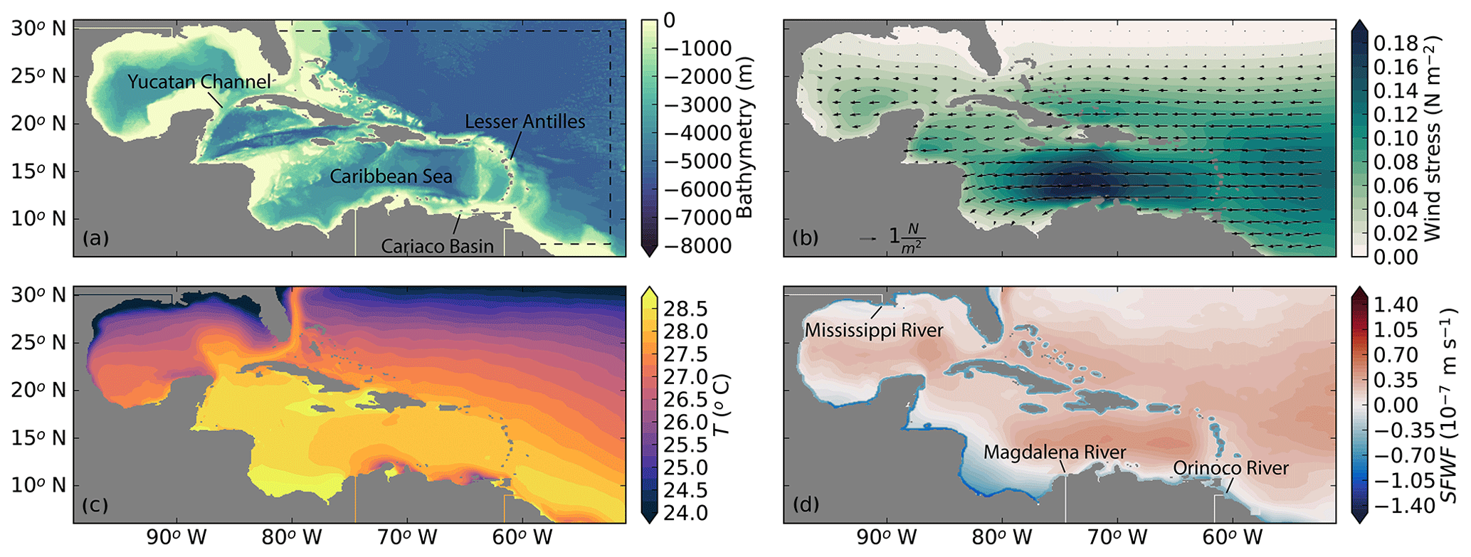
Figure 1 Setup of the regional model in MITgcm. (a) Bathymetry in meters. The sponge layer is indicated with the dashed line. (b) Magnitude of the wind stress. The direction in indicated with the vectors. Not all velocity vectors are shown for clarity purposes. (c) Surface temperature field (^∘C) used for restoration. (d) Surface freshwater flux (m s⁻¹). Positive values correspond to a net surface buoyancy loss.

All simulations were forced with time-averaged surface and lateral boundary conditions. A sponge layer with a meridional width of 1.25^∘ (15 grid cells) was applied at the lateral boundaries. There, the velocity fields were relaxed towards the time-averaged fields of Mercator (years 2007–2017) with a relaxation time that varied linearly from a month at the offshore side of the domain towards a day at the domain boundary. At these boundaries, temperature, salinity, and velocities in the zonal and meridional directions were prescribed. At the surface, a freshwater flux, temperature restoration, and a wind stress were applied (Fig. 1b–d). The temperature was restored towards sea-surface temperature (SST) averaged over the years 2007–2017 of Mercator with a relaxation timescale of 1 month. The surface freshwater flux was obtained from the diagnosed freshwater flux of a 250-year simulation described in Le Bars et al. (2016). The Orinoco River, Magdalena River, and Mississippi River are prescribed as stationary freshwater fluxes at the open boundaries with discharges based on Fekete et al. (2000).

The reference simulation (Ekman100) is forced by a time-averaged zonal wind forcing computed from the wind fields of years 2007–2017 of ERA-Interim (Dee et al., 2011). Prescribing stationary values implied that the NBC Rings, which can trigger the formation of the anticyclones (Goni and Johns, 2003; Richardson, 2005), were not represented at the boundaries. However, Jouanno et al. (2009) and Lin et al. (2012) showed that a realistic eddy field in the Caribbean Sea can be obtained without the presence of NBC Rings. Moreover, in Sect. 3 we will show that a realistic eddy field is obtained with these boundary conditions. Therefore, we considered these boundary conditions sufficient for the purpose of this study.

To investigate the effect of wind-driven upwelling on the westward intensification of anticyclones, only this zonal wind forcing (τ_x) was altered between simulations. The magnitude of the zonal wind stress was reduced or increased in each simulation by the same constant over the entire domain (Fig. 2). With this approach, we ensured that we only change the upwelling strength and not the curl of the wind stress. The magnitude of the reduction or increase was determined based on the zonal wind stress in the upwelling region in Ekman100. In Ekman150, the zonal wind stress in the upwelling region was 50 % stronger than the wind stress in Ekman100, resulting in a theoretical increase in the northward Ekman transport of 50 %. The wind stress along the coast was weaker in Ekman50, leading to a theoretically weaker upwelling (50 %) in this simulation compared to Ekman100. The same principle was applied in Ekman75 and Ekman125.

Figure 2 Average zonal wind stress (N m⁻²) in the southern Caribbean Sea (10.5–12.5 ^∘N, 65–70 ^∘W) in the simulations. The seasonal variation of the zonal wind stress at this location, obtained from ERA-Interim (Dee et al., 2011), is shown for reference. Negative values correspond to easterly winds.

The adjustment of the zonal wind forcing resulted in changes in mesoscale variability over the full domain. Because the applied constant was optimized to alter the northward Ekman transport in the Cariaco and Guajira upwelling regions, it resulted in unrealistic magnitudes of the zonal wind stress (and thus of the northward Ekman transport) in some other regions. Therefore, we will only analyze the impact of the changes in wind forcing on the mesoscale variability close to the Cariaco and Guajira upwelling regions (Fig. 3c) and disregard other coastal upwelling regions.

The range of τ_x applied in the simulations covers the seasonal variations (Fig. 2). The magnitude of the stationary zonal wind stress in Ekman50 was similar to the observed zonal wind stress in fall, while the stronger stationary zonal wind stress in Ekman125 was comparable to the wind stress during winter and summer months. The zonal wind stress in Ekman150 was stronger than the seasonal cycle but was similar to zonal wind stresses that are observed during years with anomalously high wind velocities (Whyte et al., 2008).

2.2 Methods

To analyze the behavior of the mesoscale eddies, we analyzed both the eddy kinetic energy (EKE) and the individual eddies. Following Jouanno et al. (2012), we calculated the EKE from 5 d averaged velocity fields that were high-pass filtered with a 125 d running mean. This 125 d period was long enough to capture the variability of the eddies, which have a characteristic period of 50–100 d (Jouanno et al., 2008), but was shorter than the interannual variability.

To gain insight into the westward intensification of Caribbean anticyclones, we used the py-eddy tracker to follow them (Mason et al., 2014). The py-eddy tracker used 5 d averaged sea-level anomaly fields to identify near-circular features. Anomalies were computed with respect to 20-year averaged fields. Negative anomalies were identified as cyclones and positive anomalies as anticyclones. More detailed information about the numerics of the py-eddy tracker can be found in Mason et al. (2014). We set a minimum lifetime of 75 d. Taking into account the average westward propagation velocity of 0.13 m s⁻¹ (Richardson, 2005), the anticyclones propagate approximately 840 km during this minimum lifetime.

At the center of the eddies provided by the eddy tracker, we extracted the amplitude (A_eddy), swirl velocity (u_swirl), radius (R_eddy), and properties from the model output to assess their characteristics. The amplitude was defined as the sea-surface height difference between the eddy and the 20-year average sea-surface height at the center of the eddy. Since the py-eddy tracker identifies circular anomalies as eddies, we could define the swirl velocity as the average of the maximum northward and maximum southward velocity of the eddy. The location of both velocities was used to obtain a robust estimate of the eddy radius (R_eddy), which we defined as half the distance between these locations. To characterize the local properties (T, S, σ) of the background and the eddies, these variables were averaged over the upper 50 m. This depth corresponds to the average depth of the pycnocline in the Caribbean Sea. The latter ensures that these properties not only reflect variations in surface forcing. The background properties were defined as the 125 d averaged values of the upper 50 m at the location of the eddy obtained from the py-eddy tracker. The differences between the properties of the eddies and the background are computed as $\mathrm{\Delta }=\mathrm{eddy}-\mathrm{background}$.

To gain insight into the geostrophic part of the westward intensification of the anticyclones in each simulation, we computed the strength of the horizontal density gradients ($\left|\mathrm{\nabla }\mathit{\sigma }\right|$). These gradients were calculated over the upper 50 m of the water column for 5 d averaged density fields as follows:

$$\begin{array}{}\text{(1)}& \left|\mathrm{\nabla }\mathit{\sigma }\right|=\sqrt{{\left({\displaystyle \frac{\partial \mathit{\sigma }}{\partial x}}\right)}^{\mathrm{2}}+{\left({\displaystyle \frac{\partial \mathit{\sigma }}{\partial y}}\right)}^{\mathrm{2}}},\end{array}$$

where σ is the density. The contribution of temperature ($\left|\mathrm{\nabla }{\mathit{\sigma }}_T\right|$) and salinity ($\left|\mathrm{\nabla }{\mathit{\sigma }}_S\right|$) to the horizontal density gradients was computed in a similar manner, whereby the density differences were calculated assuming a linear equation of state as $\mathrm{\Delta }{\mathit{\sigma }}_T={\mathit{\rho }}_{\mathrm{0}}\mathit{\alpha }(T_{\mathrm{1}}-T_{\mathrm{0}})$ and $\mathrm{\Delta }{\mathit{\sigma }}_S={\mathit{\rho }}_{\mathrm{0}}\mathit{\beta }(S_{\mathrm{1}}-S_{\mathrm{0}})$, respectively. Here, α, β, and ρ₀ are constants: $\mathit{\alpha }=-\mathrm{3.1}\times {\mathrm{10}}^{-\mathrm{4}}$ ^∘C⁻¹, $\mathit{\beta }=\mathrm{7.2}\times {\mathrm{10}}^{-\mathrm{4}}$ psu⁻¹, and ρ₀=999.8 kg m⁻³.

Since the focus of this study is to analyze the westward intensification of the anticyclones, we not only calculate the EKE and strength of the horizontal density gradients over the full domain, but we also calculate their contribution associated with the anticyclones only. We estimate the latter by considering the EKE and density gradients around the core of an eddy at each 5 d averaged field over a spatial extent of 1.5×R_eddy. This procedure allows us to study only the westward intensification of the anticyclones.

3 Performance of the regional model

3.1 Mean flow

The modeled surface current in Ekman100 enters the Caribbean Sea through the southern passages of the Lesser Antilles (Fig. 3a), which is similar to what is seen in observations (Johns et al., 2002). The flow through the Lesser Antilles is highly variable and depends on variations of the flow upstream and the wind forcing (Johns et al., 2002). Based on scarce data, Johns et al. (2002) estimated the transport at 66^∘ W as 18.4±4.7 Sv. In our simulation, the transport is more stable due to the stationary forcing and is on average 13.6 Sv at 66^∘ W, which is close to the lower range of the estimate of Johns et al. (2002). Further westward at 80^∘ W, the modeled flow accelerates over shallow topography at 17^∘ N, where it continues northwestward towards the Yucatán Channel into the Gulf of Mexico.

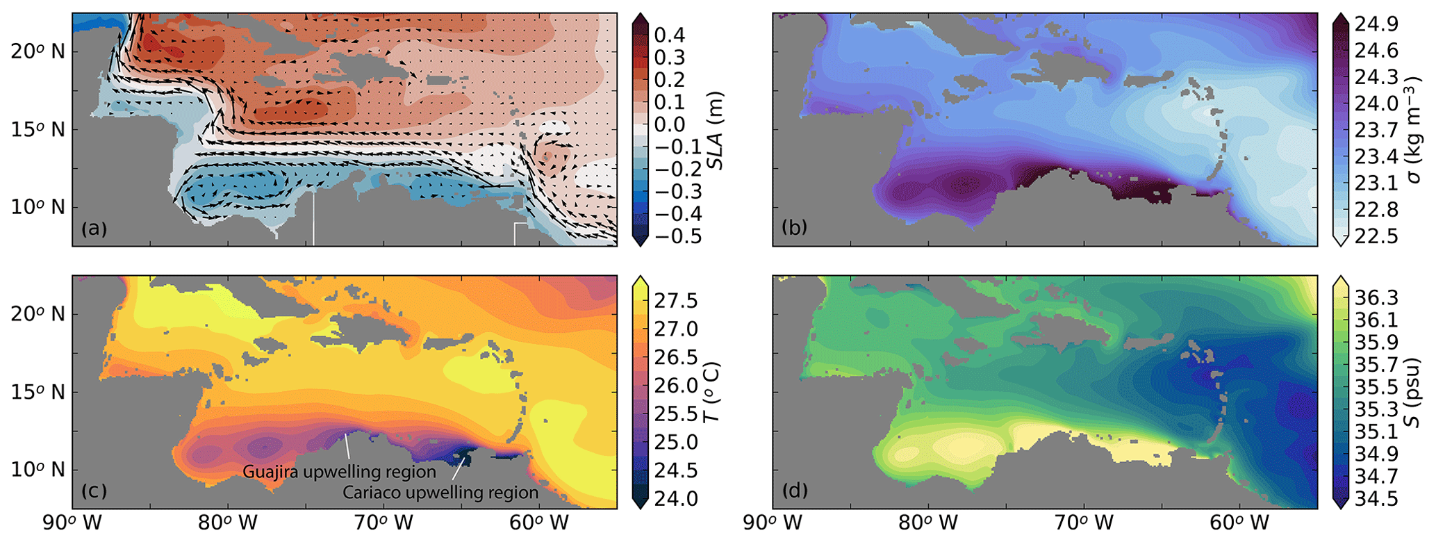
Figure 3 The 20-year near-surface average properties of the Caribbean Sea in Ekman100. (a) Mean sea-level anomaly (SLA) in meters with velocity vectors. Surface current vectors are only shown every eighth grid cell for clarity purposes. (b) Density ($\mathit{\sigma }=\mathit{\rho }-\mathrm{1000}$; kg m⁻³), (c) temperature (^∘C), and (d) salinity (psu). Properties in panels (b, c, d) are averages over the upper 50 m.

In the southwest of the Caribbean Sea, the modeled surface currents display a cyclonic recirculation (Fig. 3a). This recirculation is known as the Panama–Colombia Gyre (PCG) and is wind-driven (Centurioni and Niiler, 2003; Andrade et al., 2003). Part of the PCG continues as an eastward subsurface countercurrent, which results from the Sverdrup circulation in the North Atlantic tropical cell (Andrade et al., 2003). The countercurrent flows below the upwelling region, and its depth is related to the wind strength (Andrade et al., 2003; Andrade and Barton, 2005). The model is able to reproduce the subsurface countercurrent at a depth of approximately 100 m, which is slightly higher in the water column than at the 200 m observed by Andrade et al. (2003) and the 150 m observed by Hernandez-Guerra and Joyce (2000); the modeled strength (0.11 m s⁻¹) is comparable to their observations.

Ekman100 displays a strong meridional density gradient in the mixed layer that varies between σ=25.1 kg m⁻³ in the south (11^∘ N) and σ=22.7 kg m⁻³ in the north (18^∘ N, Fig. 3b). The strongest meridional gradients are close to the surface and colocated with the Caribbean Current. The location of the dense waters coincide with the two major upwelling regions: Cariaco and Guajira. The upwelled waters are colder and more saline than the surrounding surface waters (Fig. 3c, d).

The Cariaco upwelling region in the southeast of the Caribbean Sea is located at 63–65^∘ W, 10–12.5^∘ N (Rueda-Roa and Muller-Karger, 2013). The modeled minimum (24.9 ^∘C) and maximum temperatures (27.4 ^∘C) in the Cariaco Basin are less extreme than the observed temperatures (minimum: 20.3 ^∘C, maximum: 30.1 ^∘C;  Rueda-Roa and Muller-Karger, 2013). Although the model is not able to capture this seasonal variability, the modeled average SST (25.4 ^∘C) is similar to observations (25.2 ^∘C; Rueda-Roa and Muller-Karger, 2013). Note that these modeled temperatures are lower than the restoring temperature (Fig. 1c), which indicates that the model is able to reproduce coastal upwelling. The Guajira upwelling region is located west of the Cariaco upwelling region between 69 and 74^∘ W (Andrade and Barton, 2005; Rueda-Roa and Muller-Karger, 2013). Here, the observed average SST is slightly higher (25.5 ^∘C) than in the Cariaco upwelling region (Rueda-Roa and Muller-Karger, 2013). Similar to these observations, the model displays a temperature difference between the two upwelling regions (26.1 ^∘C in Guajira; Fig. 3c). Furthermore, the modeled temperatures are in line with Andrade and Barton (2005), who found surface temperatures varying between 25.6 and 28 ^∘C in the Guajira upwelling region.

In addition to the meridional density gradient, the model also displays a clear zonal density gradient in the Caribbean Sea (Fig. 3b): the Caribbean Current is relatively light as it enters the Caribbean Sea. This zonal density gradient is mainly due to a zonal salinity gradient and to a lesser extent to a zonal temperature gradient (Fig. 3c–d). As mentioned in the Introduction, the zonal temperature and salinity gradients are related to the offshore advection of cold and saline upwelling filaments (Jouanno and Sheinbaum, 2013). The magnitude of the zonal density gradient is largest in the surface mixed layer and decreases rapidly below. According to observations, the zonal salinity gradient is also related to the dispersal of the Amazon and Orinoco River plumes into the basin (e.g., Hu et al., 2004; Chérubin and Richardson, 2007). In the model, the Amazon River plume enters the domain at the southern boundary, while the fresh water of the Orinoco River enters the domain at 61^∘ W, 9^∘ N (Fig. 1d). The river plume is advected with the mean flow and becomes more saline through mixing with the saline (upwelled) surface waters in the basin, as well as through evaporation. Overall, the zonal and meridional gradients of salinity and temperature are similar to observations, indicating that the model is able to capture the upwelling, the advection of the river plume water, and the relevant mesoscale processes.

3.2 Eddy kinetic energy

In line with observations (Andrade and Barton, 2000; Richardson, 2005; Carton and Chao, 1999), we find that the flow in the Caribbean Sea is highly variable (Fig. 4). In the eastern part of the basin, the modeled surface EKE is relatively low (100–300 cm² s⁻²; Fig. 4a) and similar to observations of Andrade and Barton (2000). The EKE increases westward towards a maximum >900 cm² s⁻² at 78^∘ W. The modeled magnitude of EKE is higher than found in satellite altimetry (>600 cm² s⁻²; Andrade and Barton, 2000; Jouanno et al., 2012), but it is more similar to estimates obtained from surface drifters (>900 cm² s⁻²; Richardson, 2005). This is in line with other modeling studies (Jouanno et al., 2008, 2012), and this discrepancy is mainly attributed to the coarse resolution (0.25^∘) of the gridded altimetry data products (Jouanno et al., 2008). The modeled spatial variability of EKE matches analyses of satellite altimetry well (Jouanno et al., 2012; Ducet et al., 2000). Corresponding to observations (Silander, 2005; van der Boog et al., 2019), we find that the eddy kinetic energy is surface intensified (Fig. 4b). In line with the modeling results of Jouanno et al. (2008), the magnitude of EKE at depth also increases towards the west (Fig. 4b).

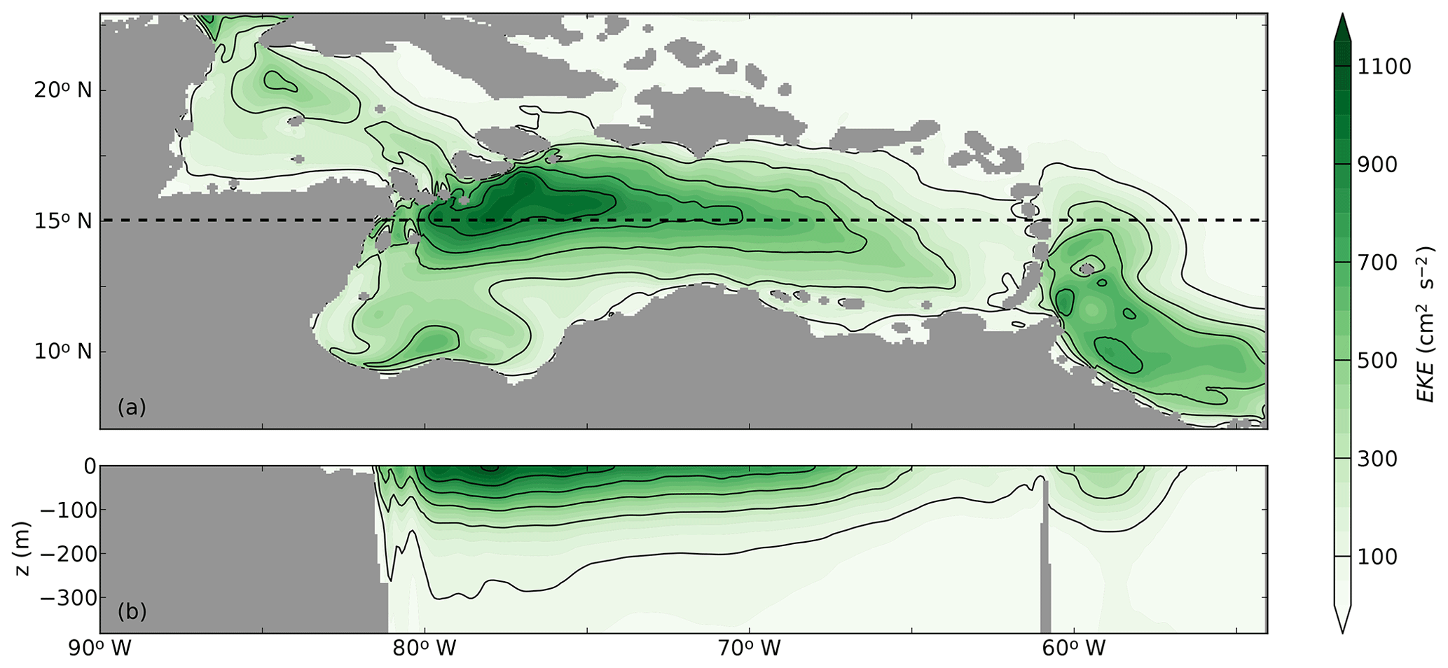
Figure 4 Eddy kinetic energy (EKE; cm² s⁻²) of Ekman100 obtained from 5 d averaged velocity fields that are high-passed filtered with a 125 d mean. (a) The 20-year average of the EKE in the upper 50 m of the water column and (b) a cross section of EKE at 15^∘ N over the upper 400 m.

The variability in the Caribbean Sea manifests itself in the presence of mesoscale eddies (Fig. 5). In line with observations (Centurioni and Niiler, 2003), the mesoscale eddies are predominantly anticyclonic (Fig. 5a). As expected, the surface densities of these anticyclones are lighter than those of the surrounding surface waters (Fig. 5b). The density differences are due to both temperature and salinity (Fig. 5c, d). Figure 5c also displays the northward advection of a cold filament. Similar filaments have been observed, and it is known that these can be advected several hundred kilometers from the upwelling region (Andrade and Barton, 2005). This advection results in the offshore cooling of surface waters (Jouanno and Sheinbaum, 2013).

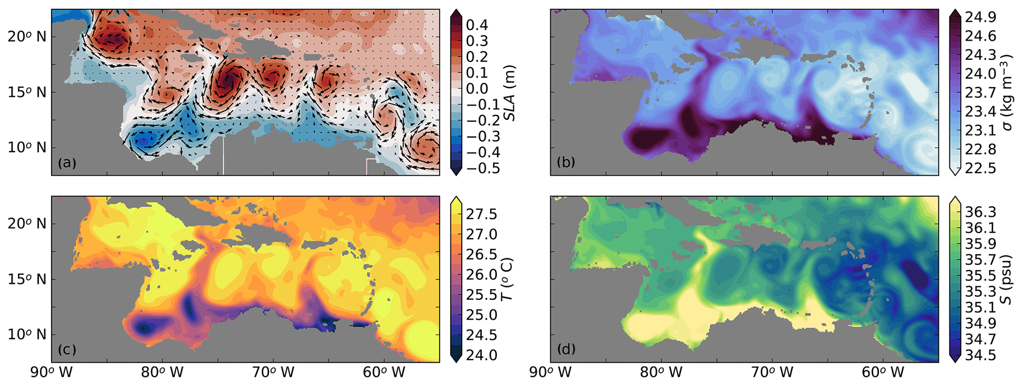
Figure 5 Near-surface properties of the Caribbean Sea averaged over a 5 d period during the final year of the simulation Ekman100. (a) Mean sea-level anomaly (SLA, in meters) with velocity vectors. Surface current vectors are only shown every eighth grid cell for clarity purposes. (b) Density ($\mathit{\sigma }=\mathit{\rho }-\mathrm{1000}$; kg m⁻³), (c) temperature (^∘C), and (d) salinity (psu). Properties averages over the upper 50 m.

3.3 Eddy characteristics

From the py-eddy tracker (Mason et al., 2014), we found that on average 8.55 anticyclones and 5.70 cyclones are formed in the reference simulation Ekman100 east of 75^∘ W between 12.5 and 17.5^∘ N every year. These numbers are in line with the 8–12 anticyclones per year estimated from surface drifter data (Richardson, 2005). To our knowledge, there are no previous estimates for the formation rate of cyclones in the Caribbean Sea.

The anticyclones have an average amplitude of A_eddy=0.17 m and swirl velocities of u_swirl=0.60 m s⁻¹ between 65–75^∘ W and 12.5–17.5^∘ N (Table 1). These amplitude and swirl velocity values are similar to those found in hydrographic surveys (Silander, 2005; Rudzin et al., 2017; van der Boog et al., 2019) and similar to velocities obtained from surface drifters (u_swirl=0.5 m s⁻¹; Richardson, 2005). In general, the core of the anticyclones is warmer ($\mathrm{\Delta }T=+\mathrm{0.15}$ ^∘C) and fresher ($\mathrm{\Delta }S=-\mathrm{0.18}$ psu) than the surrounding surface waters (Fig. 5c–d).

Table 1 Number of eddies per year and average Rossby number with standard deviations in each simulation between 12.5–17.5^∘ N and 65–75^∘ W. Amounts are obtained with the py-eddy tracker. The formation rate is computed as the number of eddies that are formed each year east of 75^∘ W. The long tracks represents the percentage of the eddies that were formed east of 65^∘ W and could be tracked west of 75^∘ W. The Rossby number is calculated as $Ro=u_{\mathrm{swirl}}/(R_{\mathrm{eddy}}*f)$, where u_swirl is the swirl velocity of the eddy, R_eddy is the radius, and f the Coriolis parameter. Density, temperature, and salinity are taken at the core of the anticyclones; 1 standard deviation is added to indicate the interannual variability.

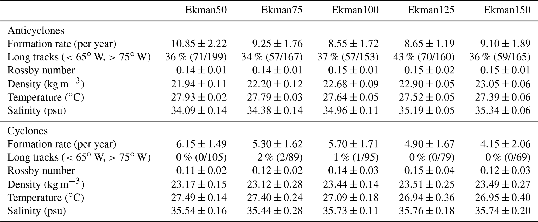
In the central Caribbean Sea (65–75^∘ W and 12.5—17.5^∘ N), the cyclones are less energetic than the anticyclones and have an average amplitude of $A_{\mathrm{eddy}}=-\mathrm{0.16}$ m and swirl velocity of u_swirl=0.50 m s⁻¹. Observations indicate that cyclones are generated near topographic features in the Caribbean Sea (Richardson, 2005) and can contain upwelling waters (Andrade and Barton, 2005). The modeled properties of the cyclones are in agreement with these observations. It appears that the mesoscale eddies are close to geostrophic balance, with an average Rossby number of 0.15±0.01 (anticyclones) and 0.14±0.03 (cyclones), where the Rossby number is calculated as $Ro=u_{\mathrm{swirl}}/(R_{\mathrm{eddy}}*f)$, in which u_swirl is the swirl velocity of the eddy, R_eddy is the radius, and f the Coriolis parameter.

There is a strong and significant correlation between the amplitude of the tracked mesoscale eddies and the surface EKE. This suggests that the westward increase in EKE is related to the strength of the eddies. We find that 57 of the anticyclones that are formed in the Caribbean Sea during the 20 years of the simulation propagate from a region with weak EKE (<65^∘ W) towards a region with high EKE (>75^∘ W). The paths of these anticyclones are indicated with the black lines in Fig. 6a. The other 96 anticyclones that are formed in the Caribbean Sea during the 20 years of the simulation are either generated west of 65^∘ W or do not pass 75^∘ W (grey lines in Fig. 6a). In contrast to the anticyclones, cyclones display relatively short tracks: only one cyclone passes both 65 and 75^∘ W (black line in Fig. 6b). This is similar to the observations of Richardson (2005), who showed that the cyclones follow a different path than anticyclones.

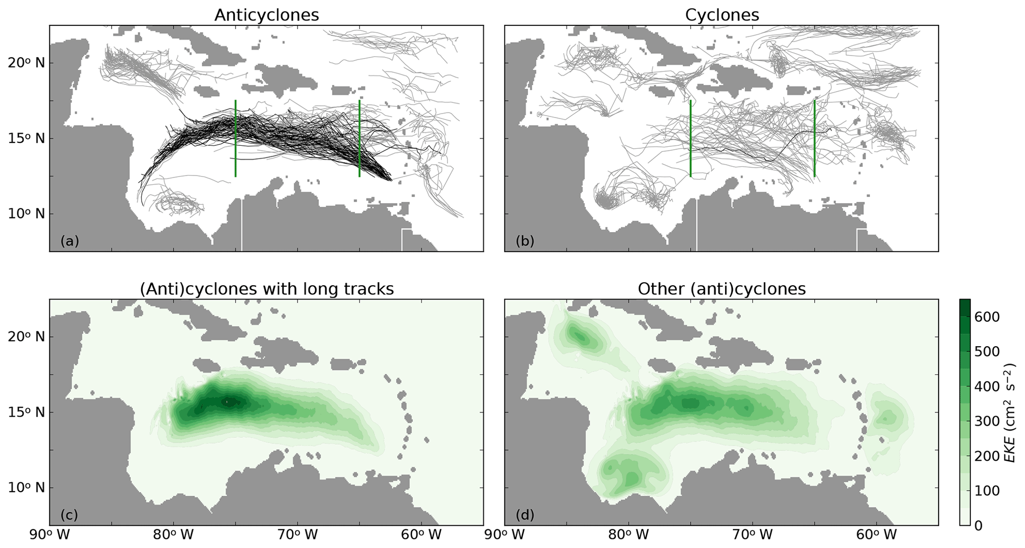
Figure 6 Paths of (a) anticyclones and (b) cyclones that are identified by the py-eddy tracker (Mason et al., 2014) in Ekman100 during 20 years of model simulation. The black lines indicate tracks that pass both cross sections at 65 and 75^∘ W (green lines). All other tracks are indicated in grey. (c) Estimate of EKE (cm² s⁻²) of the long tracks (black lines in panels a and b). (d) Estimate of EKE of all other tracks (grey lines in panels a and b).

To assess the contribution of the anticyclones with the long tracks to the total EKE variability, we calculated their EKE from the zonal and meridional velocity fields by taking into account the EKE within a region of 1.5×R_eddy around each eddy as described in Sect. 2. The spatial distribution of EKE due to these long-lived eddies (Fig. 6c) is similar to the spatial distribution of the total EKE (Fig. 4a). Notably, the magnitude of the EKE of these selected eddies is approximately 55 % of the total EKE (Fig. 4), while it is computed from only 37 % of the eddies (57 out of 153 anticyclones in 20 years). This shows that the modeled westward increase in EKE is dominated by the westward increase in EKE of a small number of long-lived eddies, which is also confirmed by the weaker eddy kinetic energy of the eddies with shorter tracks (Fig. 6d). Because our results show that the eddies with long tracks dominate the mesoscale variability in the Caribbean Sea, we will focus on these 57 energetic anticyclones in the remainder of this study.

4 Westward intensification

Figure 6 shows that the EKE of the anticyclones with long tracks increases towards the west. We hypothesized that the intensification of the anticyclones was governed by a westward strengthening of the horizontal density gradients. In this section, we evaluate the evolution of the horizontal density gradients of the anticyclones and the validity of the thermal wind balance.

Figure 7 shows the different components of the thermal wind balance ($\frac{\partial V}{\partial z}$,$\frac{g}{{\mathit{\rho }}_{\mathrm{0}}f}\mathrm{\nabla }\mathit{\sigma }$) computed from high-pass-filtered density and velocity fields. As in Fig. 6c, only the anticyclones with long tracks are taken into account. The vertical shear of the anticyclones (Fig. 7a) increases from the eastern part of the basin towards the west. The horizontal density gradients of the anticyclones (Fig. 7b) have a similar magnitude and spatial distribution as the vertical shear (Fig. 7a). This indicates that, on average, the anticyclones were close to geostrophy. For this case, the horizontal density gradients due to salinity (Fig. 7d) are slightly stronger than the horizontal density gradients due to temperature (Fig. 7c).

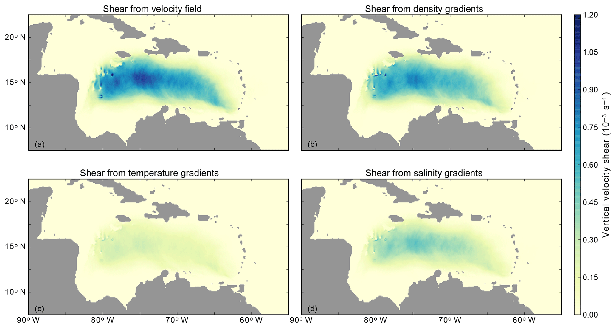
Figure 7 (a) Vertical shear of the anticyclones averaged over the upper 50 m. (b) Horizontal density gradients of the anticyclones, scaled with g∕(ρ₀f) according to the thermal wind equation. Horizontal density gradients due to (c) temperature gradients and (d) salinity gradients of the anticyclones.

To gain insight into the westward intensification of the anticyclones, we computed the zonal variation of the EKE, vertical shear, density gradients, and properties of the anticyclones (Fig. 8). Overall, the meridional maximum EKE that is contained in the anticyclones increases from approximately 200 cm² s⁻² at 65^∘ W towards 530 cm² s⁻² at 75^∘ W (Fig. 8a). These values are similar to those observed in Andrade and Barton (2000).

Similar to the EKE, the horizontal density gradients and vertical shear of the anticyclones increase towards the west (Fig. 8b). In line with the low Rossby number of the anticyclones, there is a small difference in magnitude between the vertical shear and density gradients, indicating the presence of small ageostrophic velocities. As in Fig. 7c and d, the horizontal density gradients due to temperature and salinity gradients both increase towards the west. This increase in both temperature and salinity can be explained by the properties of the upwelled waters, which are both colder and more saline than the background environment. Note that the density gradients induced by salinity are stronger than those induced by temperature differences (dashed and dotted lines in Fig. 7c–d, respectively). Although the anticyclones become slightly denser on their path westward through mixing with the surrounding waters (dots in Fig. 8c), this density increase is much weaker than the westward density increase of the surrounding waters (solid line in Fig. 8c), suggesting that changes in the properties of the background environment are indeed the dominant factor resulting in the westward increase in the horizontal density gradients.

Because the westward increase in the horizontal density gradients and vertical shear of the anticyclones (Fig. 8b) is not constant, we computed the variations with longitude in the westward direction of these quantities (Fig. 8d). From this, three regions can be identified as locations of more rapid intensification (64.6, 66.7, 72^∘ W). Up to 64.6^∘ W, the westward increase in horizontal density gradients is not fully balanced by the vertical shear, indicating that the westward intensification of the anticyclones is not in geostrophic balance at this stage. The westward intensification becomes more geostrophic towards the second peak of rapid intensification at 66.7^∘ W (Fig. 8d). This peak is located near the Cariaco upwelling region. As the anticyclones move closer to the Guajira upwelling region, they intensify more rapidly again (at 72^∘ W in Fig. 8d). Although the third rapid increase is located eastward of the Beata Ridge at 73^∘ W, it is possible that this topographic feature has some impact on the westward intensification, as was previously proposed by Andrade and Barton (2000). However, our model results suggest that all three regions of more rapid increase are located close to preferred locations of the shedding of upwelling filaments (Fig. 5c).

Figure 8 (a) Zonal variation of the (a) meridional maximum eddy kinetic energy, as well as (b) vertical velocity shear and shear computed from horizontal density gradients between 12.5 and 17.5^∘ N of the anticyclones with long tracks. The shaded regions indicate the 25th and 75th percentile. All properties are averaged over the upper 50 m of the water column. (c) Density anomaly of the background (σ_bg) and anticyclones (σ_AC) averaged over the upper 50 m. The density anomaly of the anticyclones is averaged per degree longitude. (d) The variations of vertical shear and horizontal density gradients with longitude in the westward direction of the anticyclones with long tracks.

5 Offshore advection of dense upwelling filaments

Figure 8 shows that the westward increase in EKE coincides with a westward increase in the vertical shear and density gradients of the anticyclones. This westward density increase of the surrounding surface waters is possibly governed by the advection of cold upwelling filaments offshore (Jouanno and Sheinbaum, 2013). According to Jouanno and Sheinbaum (2013), these filaments, characterized by strong temperature gradients, are advected by the anticyclones. Since we found regions with a more rapid increase in horizontal density gradients of the anticyclones (Fig. 8d), we evaluate in this section whether that increase is related to the advection of cold upwelling filaments.

We defined a measure for the strength of the filaments to study if there is a relation between the filaments and the eddy kinetic energy of the anticyclones. Because of their sense of rotation, the filaments are expected on the western side of the anticyclones, and hence we define this measure as a combination of the asymmetry of the density gradients around the anticyclone and the density gradient (induced by temperature) on the western side of the anticyclone. The asymmetry is defined as the ratio between the strength of the horizontal density gradient on the western and eastern side of the anticyclone ($\frac{\left|\mathrm{\nabla }{\mathit{\sigma }}_{\mathrm{west}}\right|}{\left|\mathrm{\nabla }{\mathit{\sigma }}_{\mathrm{east}}\right|}$). An asymmetry larger than 1 corresponds to a situation in which the density gradients on the western side of the anticyclone are stronger than on the eastern side, which suggests that an anticyclone advects a filament. Furthermore, we expect the anticyclones that advect filaments to have strong horizontal temperature gradients on the western side. These two properties are shown in Fig. 9a. It displays a positive correlation between the asymmetry and the strength of the temperature gradients so that the most asymmetric anticyclones have the strongest temperature gradients on their western side, corresponding to our hypothesis that the anticyclones with strong temperature gradients advect cold upwelling filaments.

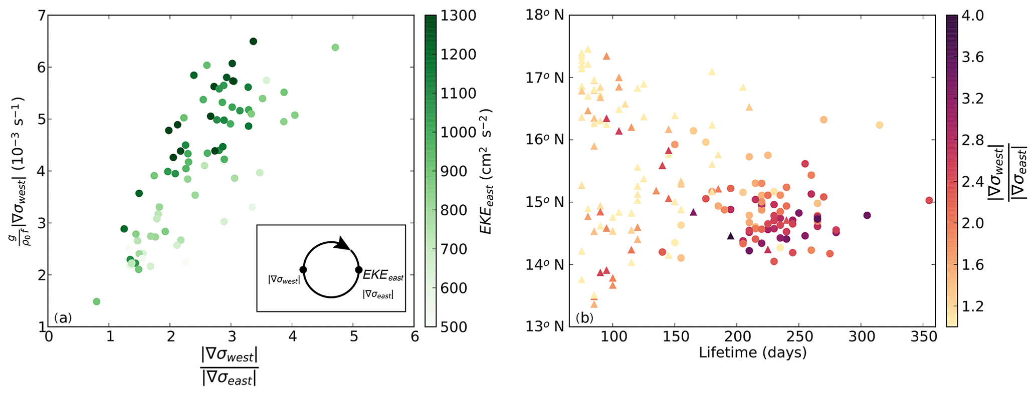
Figure 9 (a) Asymmetry of the anticyclones $\left(\frac{\left|\mathrm{\nabla }{\mathit{\sigma }}_{\mathrm{west}}\right|}{\left|\mathrm{\nabla }{\mathit{\sigma }}_{\mathrm{east}}\right|}\right)$ versus the strength of the horizontal temperature gradients on the western side of the anticyclones ($\left|\mathrm{\nabla }{\mathit{\sigma }}_{T,\mathrm{west}}\right|$) in Ekman100. The asymmetry is defined as the ratio between the strength of the horizontal density gradient on the western and eastern side of the anticyclone between 65 and 75^∘ W. Colors indicate the EKE of the eastern side of each eddy. Each dot represents one anticyclone, and the inlay contains a schematic of the locations where the properties are calculated. (b) The total lifetime versus latitude of each anticyclone. Anticyclones with long tracks (black lines in Fig. 6a) are indicated with dots, and anticyclones with short tracks (grey lines in Fig. 6a) are indicated with triangles. Colors denote the asymmetry of the anticyclones. All properties are calculated as average values between 65 and 75^∘ W from individual anticyclones in all simulations.

The relation between the eddy kinetic energy and the advection of filaments is also shown in Fig. 9a. The average eddy kinetic energy is computed on the eastern side of the anticyclone to exclude the kinetic energy associated with the filament. The EKE of the anticyclone is positively correlated with the strength of the western temperature gradient of the anticyclone, which indicates that the anticyclones with strong filaments are more energetic than the anticyclones with weaker filaments. This means that the westward intensification of individual anticyclones can be affected by the advection of cold filaments.

To understand this positive correlation between the advection of filaments and the strength of the anticyclones, we compared the anticyclones with long tracks to the other anticyclones that are present in the Caribbean Sea between 65 and 75^∘ W (black and grey lines in Fig. 6, respectively). This comparison between the asymmetry of the anticyclones, their lifetime, and their meridional location reveals two interesting aspects (Fig. 9b). First, the anticyclones with long tracks (dots in Fig. 9b) are located in the southern part of the basin (<16^∘ N). Second, the anticyclones with long tracks are in general more asymmetric than the other anticyclones (triangles in Fig. 9b).

The combination of these two aspects suggests a relation between the advection of filaments and the lifetime of Caribbean anticyclones: anticyclones that propagate close to the upwelling region are more likely to advect a cold filament that increases their western horizontal temperature gradients. Such offshore advection of dense filaments increases the horizontal density gradients, leading to the westward intensification of the anticyclones. Consequently, these anticyclones become more energetic and their lifetime increases. In contrast to the anticyclones with long tracks, the anticyclones with short tracks (triangles in Fig. 9b) are in general more symmetric and located farther north, and thus they apparently do not advect cold filaments. This suggests that anticyclones that do not advect cold filaments dissipate, deform, or merge rather than intensify. This is in line with the earlier result that the anticyclones with long tracks are more energetic than the anticyclones with short tracks (Fig. 6c, d).

6 Impacts of varying upwelling

In the previous section, we found that the westward intensification of Caribbean anticyclones is characterized by an increase in the horizontal density gradients of the anticyclones due to the advection of cold upwelling filaments by the anticyclones themselves. We expect changes in upwelling strength to result in changes in the properties of the filaments, which would affect the westward intensification of these anticyclones. To study the impacts of upwelling on this westward intensification of the anticyclones, we performed sensitivity simulations in which we altered the upwelling strength (Sect. 2). This resulted in differences in both the mean flow and mesoscale variability.

6.1 Changes in upwelling

The zonal wind stress in Ekman50 and Ekman75 was reduced compared to Ekman100 such that the wind stress in the upwelling region was 50 % and 25 % less than Ekman100, respectively. The decrease in zonal wind stress in Ekman50 and Ekman75 results in weaker upwelling and consequently warmer SST in the Cariaco Basin (Fig. 10b, c). The highest coastal temperatures are present in Ekman50. Sea-surface salinity decreased in both Ekman75 and Ekman50 compared to Ekman100 (Fig. 10b, c). This freshening is related to the presence of a subsurface salinity maximum in the Caribbean Sea due to the presence of a water mass referred to as Subtropical Underwater. This water mass is located at approximately 100 m of depth and leads to more saline upwelled waters compared to the fresher surface waters (van der Boog et al., 2019). Weaker upwelling thus results in warmer and fresher surface waters (Fig. 10b, c), and stronger upwelling results in colder and more saline surface waters (Fig. 10d, e).

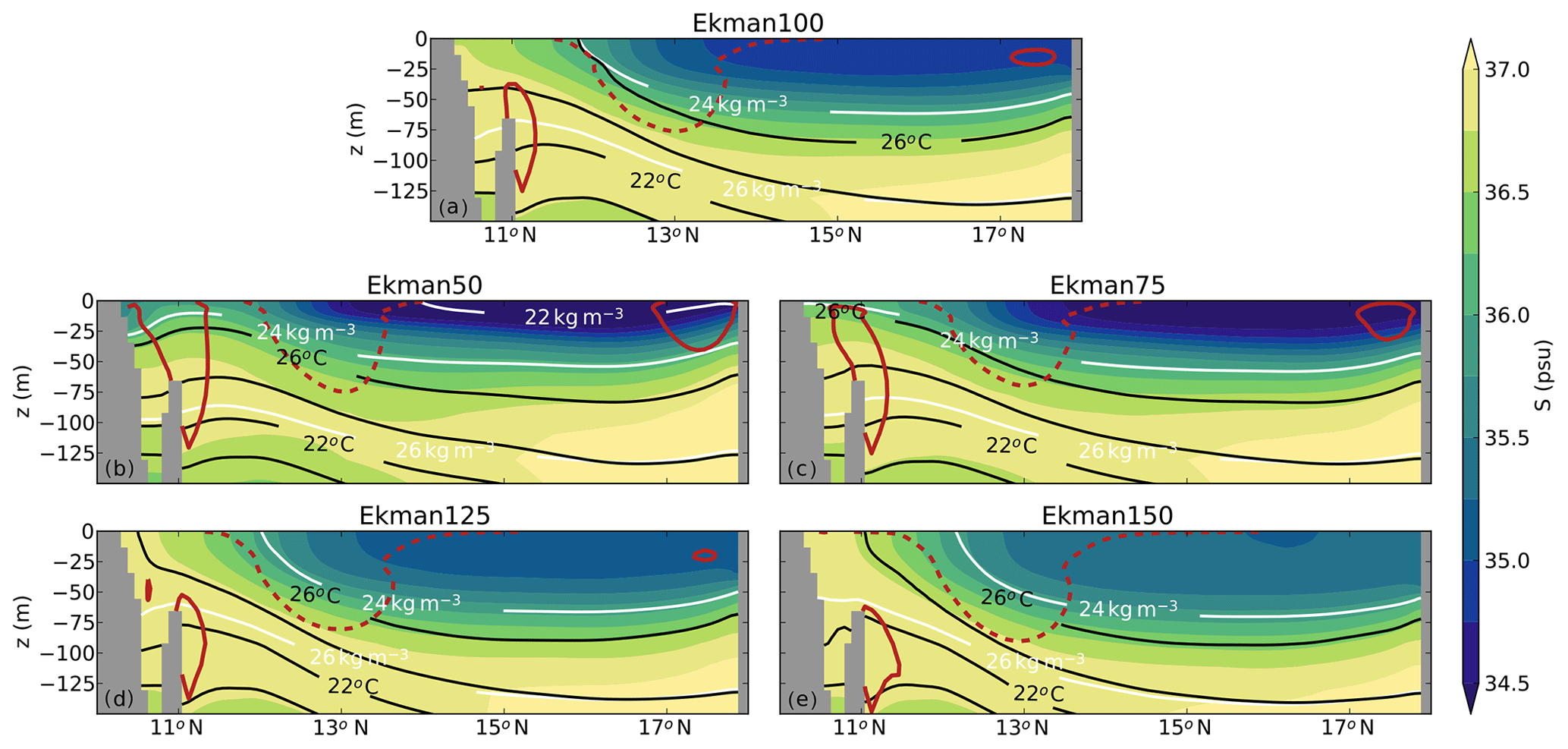
Figure 10 Cross section at 66^∘ W of the 20-year averaged salinity in (a) Ekman100, (b) Ekman50, (c) Ekman75, (d) Ekman125, and (e) Ekman150 (shading). The solid red line indicates the position of the subsurface countercurrent (contour line at an eastward velocity of 0.07 m s⁻¹). The Caribbean Current is indicated with the dashed red line (contour line at a westward velocity of 0.2 m s⁻¹). The black contour shows the 20-year average temperature in each simulation; the white contour indicates the 20-year average density in each simulation.

Besides differences in the mean properties (σ, T, S), the width of the upwelling region also changes in the simulations: in Ekman125 and Ekman150, the upwelling is confined to a narrower region than in Ekman75 and Ekman50. Moreover, we find that the core of the subsurface countercurrent is displaced upwards in Ekman50 and Ekman75 compared to Ekman100 (red contour in Fig. 10). This upward change in line with observations in which the core was also displaced upwards in weaker wind conditions (Andrade et al., 2003; Andrade and Barton, 2005). The increased northward Ekman transport in Ekman125 and Ekman150 leads to colder and more saline surface waters. In these simulations, the core of the subsurface countercurrent is positioned lower in the water column (red contour in Fig. 10). The changing position of the subsurface countercurrent and the changes in sea-surface properties in the upwelling regions indicate that the model is able to reproduce realistic upwelling properties, as also shown in Sect. 3.

6.2 Changes in EKE

The upwelling strength impacts the offshore EKE (Fig. 11). In the interior of the Caribbean Sea, the surface EKE and subsurface EKE decrease (increase) for weaker (stronger) zonal wind strength. For example, the magnitude of the mean EKE in the interior of the Caribbean Sea decreases by 27 % in Ekman50 compared to Ekman100 (Fig. 11a). In Ekman75, a slightly weaker decrease of 15 % is present (Fig. 11b). In Ekman125 and Ekman150, the surface EKE increases by 13 % and 28 %, respectively (Fig. 11c, d). Overall, the EKE variations indicate a positive correlation between the coastal wind stress and the strength of the mesoscale eddies. A similar correlation is found in the subsurface EKE. This is in line with the finding that the upwelling was shallower in the simulations with weaker upwelling and deeper in simulations with stronger upwelling.

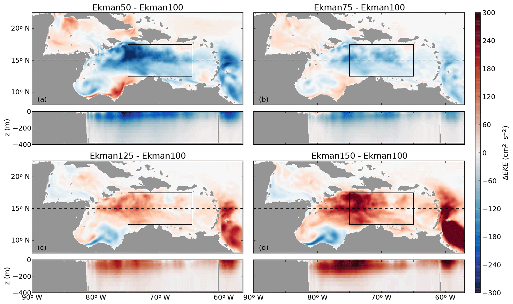
Figure 11 EKE anomaly compared to Ekman100 (Fig. 4) at the near surface and at a cross section at 15^∘ N in (a) Ekman50, (b) Ekman75, (c) Ekman125, and (d) Ekman150. Positive values correspond to enhanced EKE compared to Ekman100. The black box indicates the interior of the Caribbean Sea (12.5–17.5^∘ N, 65–75^∘ W). The dashed line shows the location of the cross sections in the lower panels.

To gain insight into the sensitivity of the westward increase in EKE to variations in upwelling, the maximum of the total EKE between 12.5 and 17.5^∘ N was computed as a function of longitude (Fig. 12a). The largest changes in EKE are seen in the western part of the basin. In Ekman100, the EKE increased by 123 % from 65 to 75^∘ W, while the weaker upwelling in Ekman50 and Ekman75 resulted in a smaller westward increase of the EKE by 62 % and 97 %, respectively. Ekman125 and Ekman150 have a stronger westward increase in EKE compared to Ekman100. Overall, there is a clear positive correlation between the upwelling strength and the westward increase in EKE.

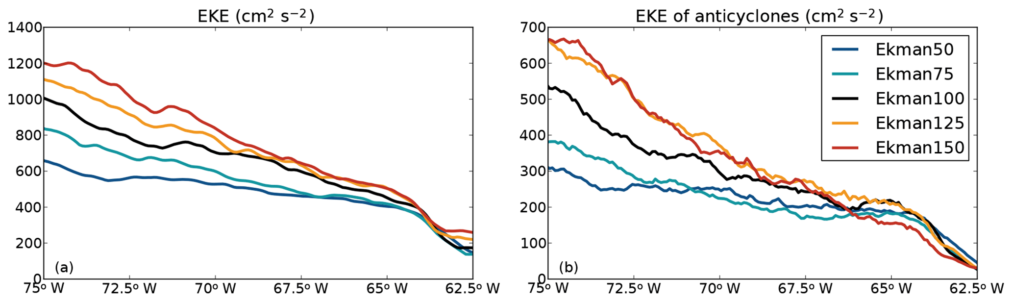
Figure 12 (a) Zonal variation of the maximum EKE between 12.5 and 17.5^∘ N from 65 to 75^∘ W for each simulation. (b) As (a), but for the anticyclones with long tracks only. The EKE was averaged over the upper 50 m. Note the difference in scale between the two panels.

6.3 Changes in eddy characteristics

Next, we assessed whether the changes in the westward increase in EKE can be attributed to changes in the eddy field and to changes in the westward intensification of anticyclones. To this end, we studied the behavior of individual eddies in each simulation with the py-eddy tracker. The number of anticyclones that are formed each year in the interior of the Caribbean Sea is highly variable and varies between 8.55 (Ekman100) and 10.85 per year (Ekman50, Table 1). These numbers are in line with a formation rate of 8–12 anticyclones per year as observed by Richardson (2005). In all simulations, between 34 % and 43 % of the anticyclones that are formed in the Caribbean Sea have long tracks (Table 1). The paths of these anticyclones with long tracks are, similar to Ekman100 (Fig. 6a), located in the southern part of the basin (not shown).

Figure 13 Zonal variation of the meridional average (12.5–17.5^∘ N) of the (a) average vertical shear of the anticyclones, (b) horizontal density gradients, (c) horizontal density gradients induced by temperature gradients, and (d) horizontal density gradients induced by salinity gradients. All properties are computed over the upper 50 m of the water column.

Similar to Ekman100, we computed the EKE associated only with the long-lived anticyclones that were formed in the eastern part of the basin (<65^∘ W) and propagate beyond 75^∘ W (Fig. 12b). Similar behavior is visible as for the total EKE in Fig. 12a: the EKE increases towards the west in all simulations, and stronger (weaker) upwelling corresponds to a larger (smaller) westward increase. In the simulations with strong upwelling (Ekman100, Ekman125, and Ekman150), the anticyclones with long tracks (Fig. 12b) are responsible for more than half of the total EKE (Fig. 12a), even though they constitute only 34 %–43 % of the total number of anticyclones in this region (Table 1). In Ekman50 and Ekman75, the anticyclones with long tracks become less dominant. In these simulations, the westward increase in EKE is also less pronounced than in the stronger wind conditions. Overall, this shows that in all simulations, a substantial part of the EKE and the longitudinal variations therein are governed by the evolution of a small number of anticyclones and that this effect is stronger in simulations with stronger upwelling.

In general, the anticyclones are fresher and warmer than the surrounding waters in all simulations. The freshest and warmest anticyclones are present in Ekman50, while the most saline and coldest anticyclones are found in Ekman150 (Table 1). It is interesting to note that the variation of the properties of the anticyclones is very small in each simulation (see the standard deviation of the anticyclone properties in Table 1). This suggests that, like shown for Ekman100 in Fig. 8c, for the simulations in which the upwelling was varied the properties of the anticyclones also remain approximately constant during their propagation westward.

In line with the observations of Centurioni and Niiler (2003), we found fewer cyclones than anticyclones in each simulation (Table 1). The lowest average formation rate of cyclones is found in Ekman150 with 4.15 cyclones per year, and the highest average formation rate is present in Ekman50 with 6.15 cyclones per year. These formation rates were highly variable, and differences in formation rates between simulations were not significant. In none of the simulations was the py-eddy tracker able to track multiple cyclones from east to west (65–75^∘ W). This implies that the cyclones are either deformed or dissipated too much such that the py-eddy tracker could not track their sea-level anomaly. Overall, the behavior of the mesoscale eddies is similar in all simulations, and the spatial pattern and magnitude of the surface EKE is governed by the anticyclones with long tracks. The westward intensification of these anticyclones is discussed in the next section.

6.4 Westward intensification

We showed in Sect. 4 that the westward increase in EKE in Ekman100 coincided with a westward strengthening of the vertical shear of the long-lived anticyclones (Figs. 6c and 7a). This increase in vertical shear was related via the thermal wind relation to the strengthening of the horizontal density gradients at the western edge of the anticyclone caused by the advection of upwelling filaments (Fig. 9a). Here, we analyze the thermal wind relation in the sensitivity simulations and its relation to the westward intensification of the anticyclones (Fig. 13).

In all simulations, the vertical shear of the anticyclones increases from east to west (Fig. 13a). This westward increase in vertical shear is similar to the westward strengthening of the horizontal density gradients (Fig. 13b). Similar to Ekman100, the magnitude of the horizontal density gradients is slightly smaller than the vertical shear in all simulations, but their variation is similar. In combination with the low Rossby number of the anticyclones (Table 1), this implies that the anticyclones are in near-geostrophic balance during their evolution.

The anticyclones display the strongest westward intensification in the simulations with stronger upwelling (orange and red lines in Fig. 13a, b). These simulations have relatively low vertical shear at 65^∘ W. In the simulations with weaker upwelling, Ekman50 and Ekman75, the anticyclones intensify less than in Ekman100. Moreover, in Ekman50, the vertical shear even weakens between 70 and 73^∘ W. At the same location, the EKE also does not increase in Ekman50 (Fig. 12b).

It is remarkable that, at 65^∘ W, the strongest vertical shear and density gradients of the anticyclones are present in Ekman50, while the weakest gradients were located in Ekman150 (compare the blue and red lines in Fig. 13a, b). This suggests that the early development (east of 65^∘ W) of the anticyclones differs between the simulations. The strong gradients in Ekman50 at 65^∘ W are surprising because we expected stronger gradients in simulations with stronger upwelling. An explanation for the strong horizontal density gradients at 65^∘ W in Ekman50 can be found after separating the total horizontal density gradients into density gradients induced by temperature and salinity (Fig. 13c, d). While the density gradients driven by temperature gradients have a similar magnitude in each simulation in the eastern part of the basin (Fig. 13c), the density gradients driven by salinity gradients differ substantially between the simulations at 65^∘ W (Fig. 13d) and are negatively correlated with the upwelling strength.

To understand why the salinity gradients in the eastern part of the basin are stronger for weaker upwelling, we analyzed the average spatial variation of the total density gradients. Figure 14 shows the magnitude of the time-averaged horizontal density gradients $\left|\mathrm{\nabla }\mathit{\sigma }\right|$ of Ekman100 (middle column) and the strengthening or weakening of these gradients in Ekman50 (right column) and Ekman150 (left column) compared to Ekman100. The strongest horizontal density gradients are located at the Guajira and Cariaco upwelling regions (Fig. 14b). These density gradients are weaker in Ekman50 than in Ekman100 (Fig. 14a) and stronger in Ekman150 (Fig. 14c).

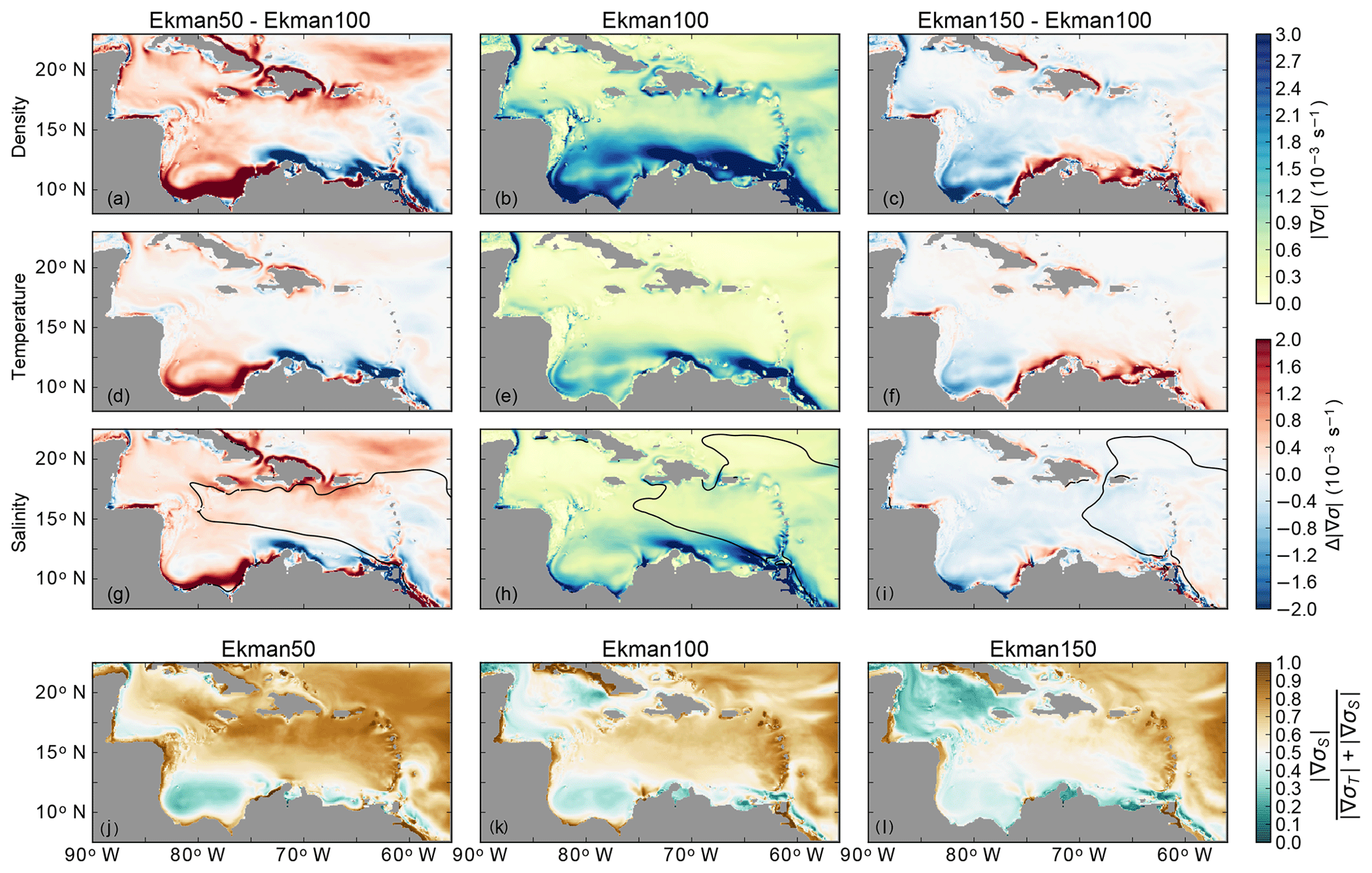
Figure 14 (a–c) Average strength of the horizontal density gradients ($\left|\mathrm{\nabla }\mathit{\sigma }\right|$) in Ekman50, Ekman100, and Ekman150 (see Sect. 2). The middle column shows the magnitude of the density gradients in Ekman100. The left and right columns show the difference between Ekman50 and Ekman100 and between Ekman150 and Ekman100, respectively. Red indicates an increase in the horizontal density gradient. (d–f) The average strength of the horizontal density gradients due to temperature variations ($\left|\mathrm{\nabla }{\mathit{\sigma }}_T\right|$). (g–i) The average strength of horizontal density gradients due to salinity variations ($\left|\mathrm{\nabla }{\mathit{\sigma }}_S\right|$). The solid black line indicates where S=35.5 psu. (j–l) The relative magnitude of density gradients due to salinity compared to density gradients due to temperature ($\frac{\left|\mathrm{\nabla }{\mathit{\sigma }}_S\right|}{\left|\mathrm{\nabla }{\mathit{\sigma }}_T\right|+\left|\mathrm{\nabla }{\mathit{\sigma }}_S\right|}$). All properties are averaged over 20 years and over the upper 50 m of the water column.

The horizontal density gradients at the upwelling region are due to both horizontal temperature and salinity gradients (Fig. 14e–h). Because upwelling brings relatively cold and saline waters towards the surface (Fig. 10), the strength of these density gradients increases for stronger upwelling (Fig. 14c) and decreases for weaker upwelling (Fig. 14a). In Ekman150, the strengthening of the horizontal density gradients is mainly due to temperature-induced density gradients in the upwelling region (Fig. 14f, i). In contrast, in Ekman50, the weakening of the temperature gradients (Fig. 14d) and salinity gradients (Fig. 14g) contributes roughly equally to the weakening of the total horizontal density gradients (Fig. 14a).

In the interior of the basin, the horizontal density gradients strengthen in Ekman50 compared to Ekman100 (Fig. 14a), while they are weaker in Ekman150 compared to Ekman100 (Fig. 14c). It appears that this response results from the increasing importance of the Amazon and Orinoco River plumes for weaker wind conditions. The wind affects both the propagation and spreading of the river plume. First of all, the northward Ekman transport advects the river plumes towards the north as previously observed by Molleri et al. (2010). This northward Ekman transport is weaker in Ekman50, and consequently the river plumes follow the mean flow towards the west (Fig. 14g). The stronger Ekman transport in Ekman150 results in a more northward path of the river plumes (Fig. 14i). The second consequence of changing wind conditions is the impact of the wind-driven vertical mixing. The strong zonal winds in Ekman150 induce more wind-driven mixing of the surface waters than the winds in Ekman50. As a result, salinity anomalies propagate less far westward in Ekman150 than in Ekman50. The farther advection of the river plume in Ekman50 explains why the anticyclones have stronger salinity gradients in Ekman50 than in the other simulations (Fig. 13d).

From this analysis we conclude that a weakening of the zonal wind in Ekman50 leads to an increased influence of the Amazon and Orinoco River plume compared to the other simulations. More specifically, in Ekman50, the upper ocean density gradients in the interior of the Caribbean Sea are dominated by salinity gradients (Fig. 14j), while the density gradients are predominantly temperature-driven in Ekman150 (Fig. 14l). So, depending on the zonal wind strength, the total horizontal density gradients in the Caribbean Sea are either driven by temperature or salinity gradients, which suggests that both the river plumes and the upwelling affect the variability in the basin.

7 Summary and discussion

In this study, we used a regional model of the Caribbean Sea to investigate the interaction between mesoscale anticyclones and the wind-driven coastal upwelling along the South American coast. We showed that the westward intensification of Caribbean anticyclones is driven by an increase in the horizontal density gradient between their cores and their surroundings (Fig. 7). Notably, the increase is governed by density changes in the surroundings and not by density changes within the anticyclone (Table 1). More specifically, the density of the surroundings increases through the offshore advection of cold filaments of upwelled water by the anticyclones, which in turn is governed by the passage of the anticyclones themselves. This increases the horizontal density gradient between the anticyclone and the surroundings on the western side of the anticyclone (Fig. 9a). As a result, its vertical shear increases, and the anticyclone becomes more energetic. Approximately two to four anticyclones per year showed this behavior. The anticyclones that are not associated with the advection of cold filaments strengthen this view that the westward intensification of Caribbean anticyclones is facilitated by the advection of filaments of upwelled water. These anticyclones were less energetic and had shorter life spans than the anticyclones that intensified towards the west.

Further support for this view is obtained from the series of simulations in which the strength of the upwelling was altered by adjusting the zonal wind stress (and thus the northward Ekman transport). Stronger upwelling leads to an increase in offshore cooling and thus to a stronger increase in the horizontal density gradient between the anticyclones and their surroundings. As a result, the anticyclones intensify more on their path westward compared to the case of weaker upwelling. We also found that a decrease in the northward Ekman transport in the basin allows the river plumes to advect further into the basin. This influences the early development of the anticyclones. This nonlinear response of the evolution of anticyclones to changes in upwelling highlights the fact that the horizontal density gradients in the Caribbean Sea are predominantly set by salinity gradients in the case of weak wind forcing and by temperature gradients in the case of strong wind forcing.

Previous studies in the Caribbean Sea mainly focused on either the influence of the river plumes (e.g., Hu et al., 2004; Chérubin and Richardson, 2007) or on the influence of the wind (e.g., Oey et al., 2003; Astor et al., 2003; Jouanno et al., 2009). However, based on our results, we argue that it is important to take the interaction between the pathway of the river plume and the upwelling into account when studying mesoscale variability in the Caribbean Sea.

Based on the different wind forcing in the simulations, we can speculate on the seasonal eddy variability in the Caribbean Sea: the strong zonal wind stress in winter is similar to Ekman125, and the weaker winds in fall are represented by Ekman50 and Ekman75. In Ekman150, the anticyclones intensified more than in Ekman50. This implies that during the strong wind forcing in winter the anticyclones intensify more. Furthermore, during weak wind forcing, we expect the salinity gradients of the river plume to become dominant. However, the dispersal of the Amazon and Orinoco River plumes also has a distinct seasonal cycle (Hellweger and Gordon, 2002; Chérubin and Richardson, 2007), which is absent in our model and would be an interesting topic for further study.

The results of this study also highlight some aspects of the interannual variability of the eddy field in the Caribbean Sea. In our simulations, stronger wind forcing resulted in a higher EKE in the center of the Caribbean Sea. Assuming that this relation holds on interannual timescales as well, these results suggest a positive correlation between the wind forcing and eddy variability in the interior of the basin. Jouanno and Sheinbaum (2013) used a model with seasonally varying boundary conditions and identified a similar relationship. This is also found in observations (Fig. 15), which show that sea-surface variance is higher in years with stronger zonal winds. Figure 15 also suggests that the response of the sea-surface variance to the wind stress is nonlinear: although 2010 and 2011 were years with weak zonal winds, the sea-surface variance was relatively high. It is interesting to note that the salinity in the Cariaco Basin was anomalously low in these years (Cariaco project, 2019). Taking into account the shallow depth of this salinity anomaly, it is plausible that it is related to the farther westward propagation of the river plumes as seen in Ekman50. This supports our view that both upwelling and the dispersal of the river plumes affect the mesoscale eddy field in the Caribbean Sea.

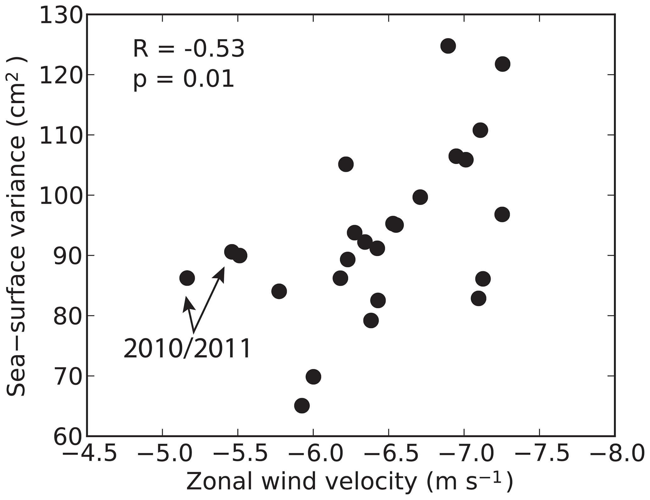
Figure 15 Year-averaged sea-level variance and coastal zonal wind velocities. Sea-surface spatial variance is obtained from daily sea-level anomaly fields from the years 1993–2017 from satellite altimetry (CMEMS) and averaged over the interior of the Caribbean Sea (12–17.5^∘ N, 65–75^∘ W). Coastal zonal winds in the upwelling region (10–12.5^∘ N, 65–75^∘ W) are obtained from the years 1993–2017 from the ECMWF (ERA-Interim; Dee et al., 2011). Each dot represents one year.

Over the past 2 decades, a weak decreasing trend has been observed in the coastal wind stress and upwelling strength (Campbell et al., 2011; Lima and Wethey, 2012; Torres and Tsimplis, 2013). Not only does this have severe ecological impacts (Villamizar and Cervigón, 2017), but it also impacts mesoscale variability. Our results suggest that weaker upwelling will lead to less westward intensification of Caribbean anticyclones and less mesoscale variability in the interior of the basin. Furthermore, in weaker wind conditions the offshore advection of (nutrient-rich) cold filaments is weaker, which results in less offshore advection of nutrients and biota.

Overall, in this study we showed how the strength of the zonal wind stress in the Caribbean Sea impacts the eddy variability in this basin. We showed how two processes induced by the northward Ekman transport impact the development of the most energetic anticyclones. First, the river plume sets the properties of the anticyclones during their early development in the eastern Caribbean Sea. Second, the anticyclones intensify themselves by the advection of cold and saline upwelling filaments. Together these two processes explain some key aspects of the mesoscale variability in the Caribbean Sea.