the Creative Commons Attribution 4.0 License.
the Creative Commons Attribution 4.0 License.
 | 30 Sep 2019
High-resolution underway measurements of phytoplankton photosynthesis and abundance as an innovative addition to water quality monitoring programs
Machteld Rijkeboer
Alain Lefebvre
Arnold Veen
Jacco C. Kromkamp
Marine waters can be highly heterogeneous both on a spatial and temporal scale, yet monitoring programs currently rely primarily on low-resolution methods. This potentially leads to undersampling. This study explores the potential of two high-resolution methods for monitoring phytoplankton dynamics: fast repetition rate fluorometry for information on phytoplankton photosynthesis and productivity and automated scanning flow cytometry for information on phytoplankton abundance and community composition. These methods were tested in combination with an underway Ferrybox system during four cruises on the Dutch North Sea in April, May, June, and August 2017. The high-resolution methods were able to visualize both the spatial and temporal variability of the phytoplankton community in the Dutch North Sea. Spectral cluster analysis was applied to objectively interpret the multitude of parameters and visualize potential spatial patterns. This resulted in the identification of biogeographic regions with distinct phytoplankton communities, which varied per cruise. Our results clearly show that the sampling based on fixed stations does not give a good representation of the spatial patterns, showing the added value of underway high-resolution measurements. To fully exploit the potential of the tested high-resolution measurement setup, methodological constraints need further research. Among these constraints are accounting for the diurnal cycle in photophysiological parameters concurrent to the spatial variation, better predictions of the electron requirement for carbon fixation to estimate gross primary productivity, and the identification of more flow cytometer clusters with informative value. Nevertheless, the richness of additional information provided by high-resolution methods can improve existing low-resolution monitoring programs towards a more precise and ecosystemic ecological assessment of the phytoplankton community and productivity.
- Article
(4004 KB) - Full-text XML
-
Supplement
(564 KB) - BibTeX
- EndNote


The Dutch North Sea is of major socioeconomic importance because of its close proximity to densely populated areas and its intensive utilization for shipping, fishing, sand extraction, and the development of offshore windmill farms. Due to this high anthropogenic pressure, the North Sea has undergone considerable biogeochemical and biological changes in the past decades (Burson et al., 2016; Capuzzo et al., 2015, 2017). For example, nutrient load and stoichiometry were fluctuating substantially due to the inflow of wastewater and agricultural runoff and subsequent mitigation efforts (Burson et al., 2016; Philippart et al., 2000). Additionally, water clarity decreased in large parts of the North Sea during the 20th century (Capuzzo et al., 2015). These abiotic changes affect primary productivity and community composition shifts throughout the trophic levels, with large implications for ecosystem functioning and fisheries production (Capuzzo et al., 2017; Burson et al., 2016). Over time, further changes are expected due to the planned energy transition and under the impact of climate change. Anticipated climate change effects include increasing temperatures, sea level rise, and ocean acidification. Already, the North Sea is warming more rapidly than most other seas (Philippart et al., 2011). These changing environmental conditions will have a big impact on marine biogeochemistry, phytoplankton community composition, and primary productivity (Sarmiento et al., 2004; Behrenfeld et al., 2006; Marinov et al., 2010). Changes in phytoplankton community composition and primary productivity affect the entire ecosystem and global biogeochemical cycles (Montes-Hugo et al., 2009; Falkowski et al., 1998; Schiebel et al., 2017). Systematic and sufficient monitoring of these changes is of crucial importance to recognize threats and, once identified as such, develop mitigation actions.
Although phytoplankton community composition and productivity can be highly variable on a spatial and temporal scale, governmental monitoring still consists mainly of low-resolution measurements (Baretta-Bekker et al., 2009; Kromkamp and van Engeland, 2010; Cloern et al., 2014; Rantajarvi et al., 1998). Currently, biological monitoring of phytoplankton in the Dutch North Sea is dictated by the requirements set by OSPAR and the EU Marine Strategy Framework Directive (MSFD 2008/56/EC). Samples are taken between March and October with a frequency of every 2 or 4 weeks. The phytoplankton analysis consists of high-performance liquid chromatography (HPLC) analysis of Chl a concentration, microscopy counts of Phaeocystis cells, and, at some stations, coccolithophore or toxic dinoflagellate cells. Sampling points were reduced from almost 70 in 1984 to less than 20 today, while strong seasonal patterns, high riverine input, and tidal forces make the Dutch North Sea a region with high spatiotemporal variability. Modern automated flow-through underway systems have the potential to be an effective addition to monitoring programs because they offer the opportunity to record the surface ocean with high spatial and temporal resolution. Such high-resolution methods are well established in physical oceanography, but for biological parameters the implementation has been lacking. This is mostly due to the complicated interpretation of biological parameters, resulting in high uncertainties in the current global estimates of net primary productivity (Silsbe et al., 2016). Underway measurements are not able to replace some more detailed low-resolution measurements, but their higher spatial and temporal resolutions provide the possibility to identify short-lived events, detect small-scale changes in phytoplankton dynamics, evaluate the consequences of possible (spatial) undersampling, and act as an early warning system. Additionally, underway measurements acquire information on living organisms and samples unaffected by transport, storage, or conservation. Two noninvasive, high-resolution methods with the potential to be implemented in phytoplankton monitoring programs are scanning flow cytometry (FCM) for information on phytoplankton abundance and community composition and fast repetition rate fluorometry (FRRf) to give information on phytoplankton photophysiology. Scanning flow cytometry is a method for counting and pulse-shape recording phytoplankton cells informative on size, fluorescence, and scattering properties per algal cell. Based on these characteristics cluster analysis allows for division into groups of similar pigment characteristics and size classes (Thyssen et al., 2015; Rijkeboer, 2018). The FRRf uses active fluorescence to gain insight into phytoplankton photophysiology. This technique is an alternative to traditional production–light curves (PE curves) by estimating the photosynthetic electron transport rate (or gross photosynthesis) at increasing ambient light levels (Suggett et al., 2009a; Silsbe and Kromkamp, 2012). Electron transport rate per unit volume is estimated based on the fluorescence response to a series of single turnover light flashes that cumulatively close all photosystems (Kromkamp and Forster, 2003; Suggett et al., 2003). This single turnover technique allows for the calculation of the effective absorption cross section and, in combination with an instrument-specific calibration coefficient, the number of reaction centers per volume (Kolber et al., 1998; Kromkamp and Forster, 2003; Oxborough et al., 2012; Silsbe et al., 2015). Electron transport rate per volume can be used to estimate gross primary productivity (Kromkamp et al., 2008; Smyth et al., 2004; Suggett et al., 2009a). These two methods are supplementary because the interaction of phytoplankton with their environment is always a sum of the community composition and their physiology. For instance, if waters become more turbid, phytoplankton can acclimate by increasing their effective absorption cross section, but it could also lead to a shift in community composition toward species with higher light use efficiency (Moore et al., 2006). Therefore, the combination of these two instruments allows for more in-depth analysis and understanding of ecosystem processes.
The aim of this study is to test two high-resolution methods, a pulse-shape recording flow cytometer and an FRR fluorometer, on their potential to be developed into a novel phytoplankton monitoring method. The two instruments were deployed concurrently on four 4 d cruises in April, May, June, and August to meet a wide range of environmental conditions and phytoplankton community states. These measurements allow for the quantification of temporal and mesoscale spatial patterns in phytoplankton abundance, photophysiology, and gross primary production. In this paper we provide an overview of the acquired results, use spectral cluster analysis to visualize spatial heterogeneity, and evaluate the potential of these methods to optimize current monitoring programs.
2.1 Study site and sampling
The Dutch North Sea is a shallow tidal shelf sea in the southern part of the North Sea. The main water flow is northward. Atlantic water enters the North Sea from the south via the channel and from the northeast where it curves around Scotland. Both currents meet north of the Dutch coast, forming the Frisian Front. For a detailed description on the North Sea physical oceanography, see Sündermann and Pohlman (2011). Along the Dutch coast, high river input, especially from the Rhine, decreases the salinity and loads the coastal zone with high nutrient concentrations (Burson et al., 2016). Anthropogenic pressure is high in the Dutch North Sea, resulting in a history of large shifts in nutrient concentrations and water clarity (Capuzzo et al., 2015; Burson et al., 2016).
The monitoring of the Dutch North Sea is performed by the Dutch government (Rijkswaterstaat) in a monitoring program called MWTL (Monitoring Waterstaatkundige Toestand des Lands, freely translated as “Monitoring of the status of the governmental waters of the country”). The locations of the sampling stations of the program are organized along transects (Fig. 1). The stations are sampled between March and October with a frequency of every 2 or 4 weeks, dependent on the transect.

Figure 1Sampling locations of the MWTL monitoring program referred to in this study. The stations are named according to the transect (Terschelling, Noordwijk, and Walcheren), followed by the number of kilometers from the coast (labels next to sampling points). The boundaries of the Exclusive Economic Zone (EEZ) are indicated by the grey dotted lines, and the Dutch EEZ is colored light blue. The locations of three major inflows to the Dutch North Sea are named at the corresponding locations (the Rhine, Dutch delta, and the Wadden Sea). The inset visualizes the location of the Dutch North Sea in a broader map of Europe. Figure made with QGIS v2.14.2 using EEZ zone data from the Flanders Marine Institute (2018).
In 2017, four 4 d sampling surveys (10–13 April, 15–18 May, 12–15 June, and 14–17 August) were conducted for the JERICO-NEXT project onboard the RV Zirfaea during their regular monitoring cruises on the Dutch North Sea. To assess the heterogeneity of the Dutch North Sea and the benefits associated with high-resolution monitoring, the four cruises were conducted in different months (April, May, June, and August), thereby aiming to cover different seasons and stages of the phytoplankton bloom (Baretta-Bekker et al., 2009).
The water inlet of the underway system was situated approximately 3.5 m below sea surface level. From the water inlet the sample water, with a flow rate of approximately 24 L min−1, was split towards (1) a flow-through Ferrybox (-4H-JENA engineering GmbH, Germany) equipped with an FSI Excell® Thermosalinograph (Sea-Bird Scientific, USA) to measure temperature and salinity and (2) a 230 cm3 flow-through sampling chamber (CytoBuoy BV, the Netherlands) wherein water was cleared from bubbles and sand (∼ flow rate of 1 L min−1). The time from the water inlet to the sampling chamber was approximately 2 min. A FastOcean fast repetition rate fluorometer (FRRf) with an Act2-based laboratory flow-through system (Chelsea Technologies Group Ltd, UK) and a CytoSense scanning flow cytometer (CytoBuoy BV, the Netherlands) automatically sampled from the sampling chamber every 30 min. Since the average speed of the ship was 8 knots, the average spatial resolution of FCM and FRRf measurements was 7.5 km. The Ferrybox sensors stored data every minute. During the cruises the high-resolution methods (FRRf, FCM, and Ferrybox) were combined with lower-resolution methods, consisting of measurements at 13 to 19 stations. At these stations, surface samples were taken for nutrient and chlorophyll a analyses (see Sect. 2.2) using a rosette sampler equipped with a conductivity–temperature–depth (CTD) instrument and Niskin bottles.
2.2 Chemical analyses
Samples for nutrient analyses were filtered over Whatman GF/F filters and kept frozen (−18 ∘C) until analyses. The analyses of ammonium (), nitrite (), nitrate (), phosphate (PO4), and silicate (Si) concentrations were conducted by the Rijkswaterstaat laboratory (RWS; the Netherlands) according to ISO 13395, 15681, and 16264 using a San Analyzer (Skalar Analytical B.V., the Netherlands). In the RWS internal protocol, nitrite + nitrate is measured by first reducing nitrate to nitrite using a cadmium–copper column and the addition of ammonium chloride as a buffer. Thereafter, sulfanilamide, α-naphthyl ethylenediamine dihydrochloride, and phosphoric acid are added and the extinction at 540 nm is compared to a NaNO2 standard. For measurement of ammonium concentrations first ethylenediaminetetraacetic acid (EDTA) was added to bind calcium and magnesium. Then, sodium salicylate, sodium nitroprusside, and sodium hypochlorite were added and the extinction at 630 nm was compared to a NH4Cl standard. Phosphate was measured by adding molybdate reagent and ascorbic acid to the sample and led through an oil bath at 37±2 ∘C, followed by measuring the extinction at 880 nm and comparing to a standard. Silicate concentration was measured by subsequent addition of molybdate reagent, oxalic acid, and ascorbic acid. The silicate concentration was then determined by measuring the extinction at 810 nm and compared to a silicate standard. The detection limits of the nutrient analyses were NO3NO2: 0.7 µM, Si: 0.36 µM, and : 0.03 µM.
Chlorophyll a concentration (hereafter Chl a) was determined by filtering over Whatman GF/C filters and freezing the filter at −80 ∘C. The Chl a was extracted in 20 ml 90 % acetone and centrifuged for 15 min with glass pearls (1.00–1.05 mm) using a bullet blender tissue homogenizer (Next Advance, Inc., Troy, USA) under cooling of solid CO2. The extract was analyzed in duplicate using ultrahigh-performance liquid chromatography (UHPLC). The calibration of the UHPLC system is performed every analysis day by making a 12-point standard calibration curve calculated using quadratic regression with weighting method 1 ∕ A to better distinguish smaller peaks (R2>0.995). The injection volume was 20 µL unless the concentration was below the lowest standard, in which case a second injection of 40 µL was reanalyzed. The analysis was conducted by the MUMM laboratory (Belgium) according to RWS analysis protocol A200. Quality control was performed by the RWS laboratory (the Netherlands).
2.3 High-frequency methods
2.3.1 Variable fluorescence
Variable fluorescence was measured with a FastOcean fast repetition rate fluorometer (FRRf) and Act2-based laboratory system (Chelsea Technologies Group Ltd, UK). The temperature was controlled by connecting a LAUDA Ecoline cooler (LAUDA-Brinkmann, LP., USA) to the water jacket of the Act2 system.
The acquisition protocol consisted of 100 excitation flashes with a flash pitch of 2 µs and 40 relaxation flashes with a flash pitch of 60 µs. Excitation flashes were performed with the blue LED (450 nm), and the strength of the LEDs was automatically adjusted to the phytoplankton concentration by the FastPro software. A loop of simultaneous blue and green flashes (450 nm + 530 nm) was performed after the acquisition loop of only blue LEDs in the case that the blue LEDs were not able to reach saturation (for instance, with high cyanobacteria concentrations), but as this was not the case, only the parameters measured by blue LEDs were used for further calculation. The sequence was repeated 20 times with a sequence interval of 100 ms. The sample was refreshed before each fluorescent light curve (FLC) by flushing for 60 s and kept well mixed by flushing for 200 ms between acquisition loops.
The FLC protocol consisted of 14 light steps of 100 s, the light intensity of which was automatically adjusted to get the optimal FLC shape based on the previous light curve. A pre-illumination step (55 s on 12 µ mol photons m−2 s−1) was included before the FLC to low-light acclimate the phytoplankton and to relax non-photochemical quenching (NPQ) of diatoms and other chlorophyll a and c algae as they stay in the light-activated state in the dark (Goss et al., 2006). After each light step, measurements were made in the dark for 18 s to retain a value for (minimal fluorescence in light-acclimated state). The data were corrected for the background fluorescence by taking sample blanks multiple times per day by filtration over a 0.45 µm filter and subtracting the last determined background fluorescence from the sample fluorescence.
Table 1The derived photosynthetic parameters used in the text (see Oxborough et al., 2012, and Silsbe et al., 2015, for more information). Variables used in Eqs. (1)–(8) are not included but discussed in the text.
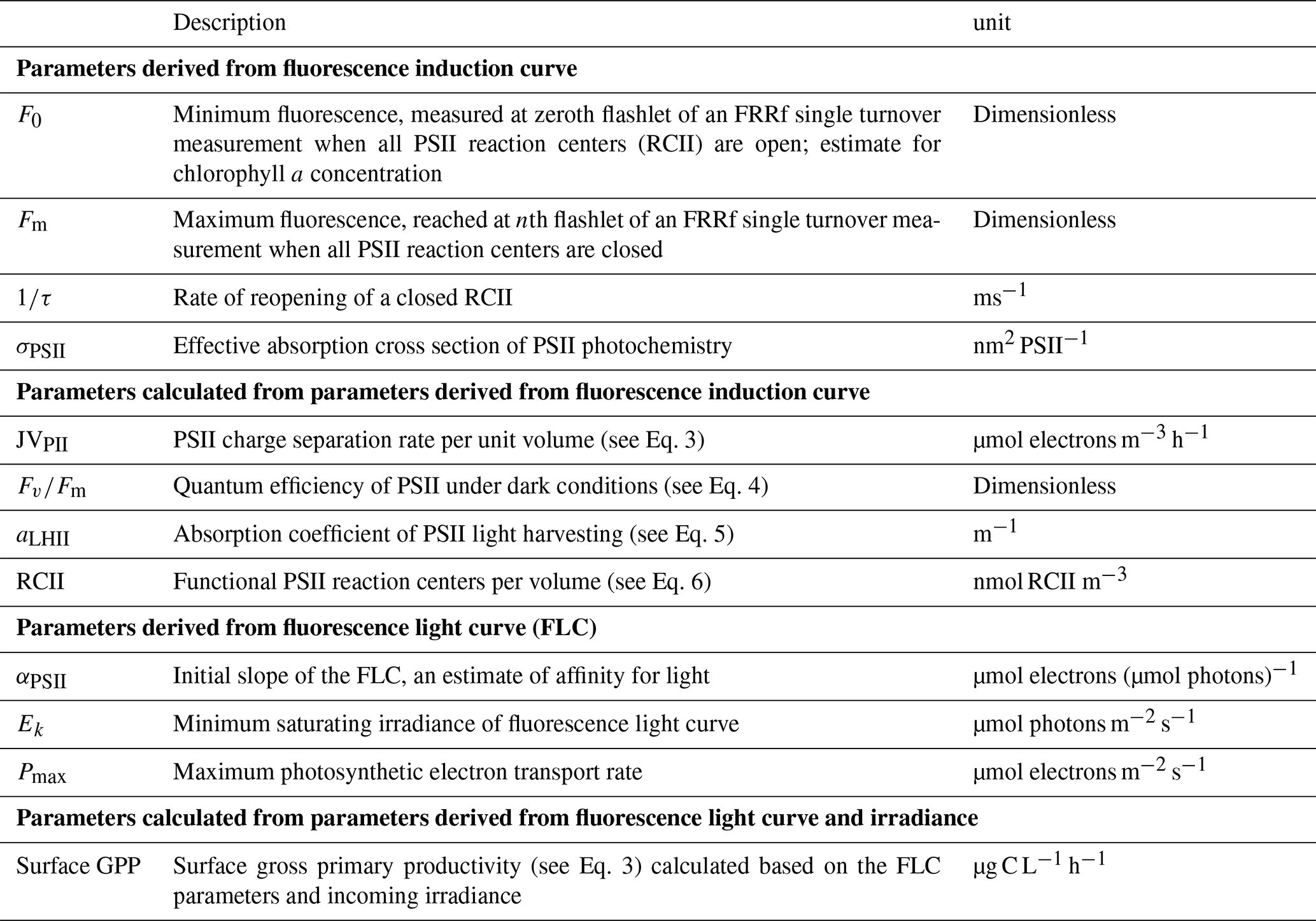
An overview of the derived photosynthetic parameters can be found in Table 1. To derive values for the maximum photosynthetic electron transport rate (Pmax), minimum saturating irradiance (Ek), and the light utilization efficiency (α) the relative electron transport rate (rETR) of the samples was fitted to the exponential model of Webb et al. (1974), after normalizing the data to the irradiance as described by Silsbe and Kromkamp (2012):
where E is the irradiance (µmol photons m−2 s−1), ' the effective quantum efficiency of photosystem II (PSII), α the initial slope of the rETR vs. irradiance curve, and Ek the light saturation parameter (in µmol photons m−2 s−1). The relative maximum rate of photosynthetic electron transport (Pmax) was calculated as
The PSII flux (µmol electrons m−3 h−1) was calculated as the product of the effective PSII efficiency (), the optical absorption cross section of the light-harvesting pigments of PSII (aLHII), and the irradiance (E):
Ka (m−1) is an instrument-specific factor necessary for obtaining absolutes rate of photosynthetic transport (see Oxborough et al., 2012, and Silsbe et al., 2015, for more information). The number of reaction centers of PSII per cubic meter (RCII) was calculated as
For more information on the calculation of RCII and aLHII, see Oxborough et al. (2012) and Silsbe et al. (2015).
QA reoxidation or the rate of reopening of a closed RCII was calculated as 1 divided by the time constant of reopening of a closed RCII with an empty QB site (τES; unit: ms−1).
Standardized daily anomalies (Z scores) were calculated for the photophysiological parameters as
Partial days were excluded because this could potentially offset the daily mean and standard deviation.
Gross primary productivity (GPP) was estimated by fitting JVPII (µmol photons m−3 h−1) to Eq. (1) (the exponential model of Webb et al., 1974) to derive a volumetric Pmax and α. GPP (µg C L−1 h−1) was then calculated using Eq. (1) and incident surface irradiance. To avoid the effects of changing incident surface irradiance (Esurface) on the spatial pattern and to be able to compare GPP between regions we used monthly average surface irradiances (Esurface) in our calculations of primary productivity. From 2010 to 2016 irradiance (400–700 nm) was measured at the roof of the NIOZ building in Yerseke using an LI-190 quantum photosynthetically active radiation (PAR) sensor and hourly averages stored using an LI1000 datalogger. Esurface was then calculated by averaging all irradiance data from the years 2010–2016 for the respective month. The primary productivity in electrons units was converted to carbon units by assuming that 6 moles of electrons were required to fix 1 mole of carbon based on a study in the adjacent Oosterschelde and Westerschelde estuaries (Jacco C. Kromkamp, personal observation, 2019).
2.3.2 CytoSense scanning flow cytometry
Single cell measurements of the phytoplankton community were conducted using a bench-top scanning flow cytometer (CytoBuoy BV, the Netherlands) equipped with two lasers (488 and 552 nm; 60 mW each). Both laser beams were ca. 5 µm high, 300 µm wide, and focused on the same spot in the middle of the flow-through chamber. The speed of the particles was ca. 2.2 m s−1. The system contained three fluorescence detector channels separating fluoresced wavelengths of 550–600 nm (FLY; phycoerythrin), 600–650 nm (FLO; phycocyanin), and above 650 nm (FLR; chlorophyll a). Additionally, the forward light scatter (FWS) and sideward light scatter (SWS) of all particles were measured. The FCM was equipped with a double set of detectors (photomultiplier tubes – PMTs) for each of the three fluorescence channels to increase the dynamic range (Rutten, 2015). Per cell, the pulse shape of the parameters (FWS, SWS, FLR, FLO, and FLY) plus their affiliates (length, total and maximum values) were recorded and saved. The instrument was checked daily for drift using 3 µm Cyto-Cal™ 488 nm alignment beads (Thermo Fisher Scientific Inc., USA). Additionally, the FCM was equipped with an image-in-flow camera to take pictures of the nanophytoplankton and microphytoplankton. This allows for linking pulse-shape recordings to microscopy results and thereby the identification of represented phytoplankton groups in the respective clusters.
Phytoplankton cells were clustered based on the pulse-shape recording of the individually scanned phytoplankton. In this paper, we discriminate the phytoplankton groups based on their size (pico, nano, and micro) and orange ∕ red fluorescence ratio (hereafter O ∕ R ratio; Table 2). The chosen cluster criteria were based on expert judgment (SeaDataNet, 2018) and corresponding to other studies (Sieburth et al., 1978; Vaulot et al., 2008). The clustering was done using the software Easyclus 1.26 (Thomas Rutten Projects, the Netherlands) according to these criteria. Noise, air bubbles, and other potential outliers were removed. The acceleration of the particles in the sheath fluid positions the cells along their long axis, which allows for size estimation based on the FWS pulse shape. A linear relation was found between length FWS and the measured length of diverse phytoplankton species (length FWS ; R2=0.98; Rijkeboer, 2018). Size estimation is limited by the width of the laser beam (5 µm), so estimations of cell sizes <5 µm are not possible based on the FWS.
Table 2The phytoplankton groups distinguished in the current study.
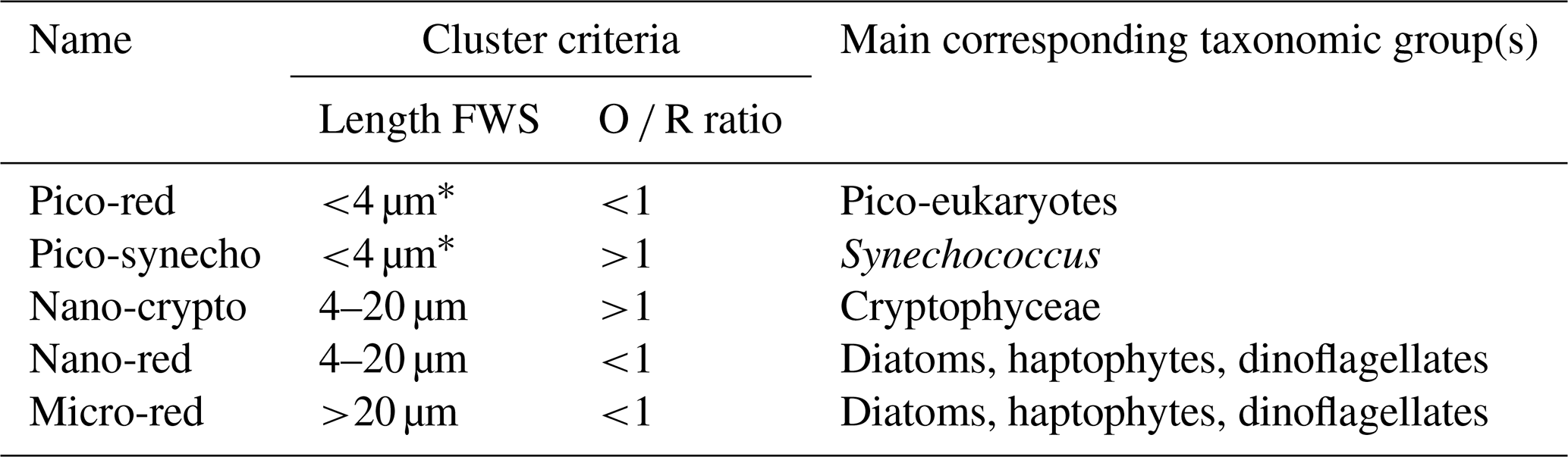
*In June <6 µm.
2.4 Data analysis
Outliers of the complete dataset were removed after visual inspection of pair plots made with the pair-plot function of the HighstatLib.V4 script (Zuur et al., 2009). For the FRRf data, quality control of the FLC fits was done based on the quality ratio of the induction curve fit per FLC light step and the r2 of the FLC fit. The quality ratio of the induction curve fit was calculated as the ratio of Fv or to the standard error (SE) of the linear regression of the saturation phase. FLC fits with an r2<0.75, or with over 30 % of the data points with a quality ratio below 6, were visually inspected and removed based on expert judgment. This led to the removal of 1 % to 7 % of the FLC fits per month. Unsatisfactory fits occurred when the auto-LED settings misadjusted the maximum irradiance or when fluorescence was too low to retrieve a reliable fluorescence signal. Especially at low biomass, FLCs became noisy, and therefore a minimum fluorescence signal was set for calculations of photosynthetic parameters. Below this blank-corrected instrument-specific fluorescence signal became noisy and often reached above the biologically unlikely limit of 0.65 (Kolber and Falkowski, 1993). The datasets of the high-resolution measurements (FRRf, FCM, and Ferrybox) were linked using corresponding time stamps. When multiple measurements were performed within one FLC, the average was used. To test whether environmental conditions (as present in the different months) had a significant effect on fluorescence as a predictor for Chl a concentration, an analysis of covariance (ANCOVA) was performed with the month as a factorial predictor. To find regions with similar phytoplankton communities, data were spectrally clustered using the uHMM R package (Poisson-Caillault and Ternynck, 2016) in the statistical software R (version 3.4.1; R Core Team, 2017). The package default settings normalize data before clustering and automatically find the number of clusters based on spectral classification and the geometry of the data. This new methodology is more robust than the classical hierarchical and k-means technics (Rousseeuw et al., 2015). Phytoplankton parameters were first tested for collinearity and predictors with a variance inflation factor (VIF) over 6 were removed (Zuur et al., 2009; see the Supplement for pair plots). This left for the cluster analysis the FCM parameters pico-red, nano-red, micro-red, and Synechococcus and the FRRf parameters σPSII, Fv∕Fm, aLHII, 1∕τ, and Ek. Data points were then labeled per cluster and plotted on a map to visually identify regions. Principal component analyses (PCAs) were performed to find which variables contributed most to the cluster results. The PCAs were based on correlation matrixes with scaled parameters to correct for unequal variances and were carried out with the prcomp() function in R (version 3.4.1; R Core Team, 2017). The PCA visualization was done using the supplemental R package factoextra (Kassambra and Mundt, 2017). Maps were made using QGIS v2.14.2, and other figures were made with ggplot2 in R (Wickham, 2009).
3.1 Abiotic conditions
Environmental conditions in the Dutch North Sea were spatially heterogeneous and differed strongly between months. Sea surface temperature increased from 9.5±1.0 ∘C in April to 19.0±0.6 ∘C in August (Table S1 in the Supplement). Differences in salinity between cruises were small, with the highest monthly mean salinity in April (34.1±1.8). The spatial variability of salinity was higher, with river influx decreasing the salinity down to 26 in the coastal zone. The monthly average of turbidity was higher in April (2.3±3.0 NTU) in comparison to other months. This was also reflected in the Kd values, which were highest in April (0.39±0.28 m−1; Table S1). It needs to be noted that monthly averages are not fully comparable because of differences in sampling route and stations (Fig. 3). Dissolved inorganic nitrogen (DIN; nitrate + nitrite + ammonium) and silicate (Si) concentrations showed spatial variability and varied per cruise (Table S2). Spatially, two trends were distinguishable: a coastal–offshore gradient and a longitudinal gradient. Per cruise the strength and position of these spatial gradients changed. The coastal to offshore gradient moved shoreward from April to August, and the southern stations were depleted earlier in the year in comparison to the more northerly stations. In April DIN and Si concentrations were on average higher and only potentially limiting (Si <1.8 µmol L−1, DIN <2 µmol L−1; Peeters and Peperzak et al. (1990) and references therein) in the most southerly part of the Dutch North Sea (Walcheren transect) and at offshore stations (>70 km offshore west of the Netherlands, >135 km north of the Netherlands). In later months, DIN and Si limitations gradually moved towards the coastal zone. Stations closest to freshwater influx (Noordwijk 2 and 10) became DIN and Si limited later in the year (Table S2). The increased DIN concentration at the transect close to the Rhine outflow was absent 70 km offshore (Noordwijk 70), suggesting that the Rhine water remained close to the coast. Phosphate concentrations were low and possibly limiting throughout the Dutch North Sea (orthophosphate <0.5 µmol L−1; Peeters and Peperzak et al., 1990), with exceptions in April north of Terschelling between 50 and 100 km offshore and in May at Noordwijk 2, a region with high freshwater influx. In June and August, phosphate concentrations recovered in the southern part of the Dutch North Sea, reaching up to 0.6 µM (Table S2).
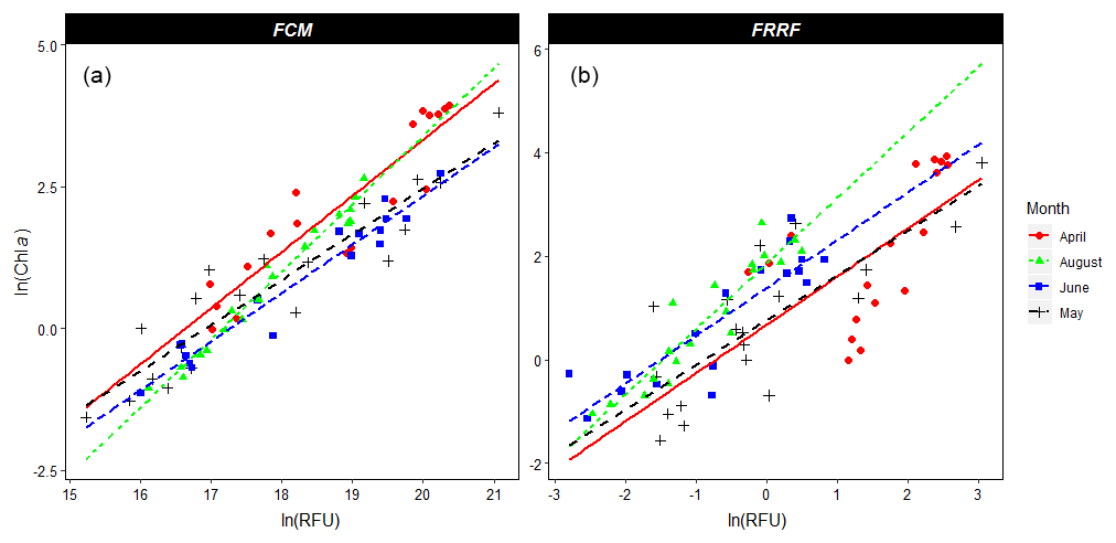
Figure 2Linear regression of the natural logarithms of Chl a concentration (µg L−1) as determined by HPLC (y axis); on the x axis is the natural logarithm of FCM-derived total red fluorescence (in relative fluorescence units – RFUs; a) and FRRf-derived minimum fluorescence (F0 in RFUs; b). Both FCM red fluorescence (p<0.01, adjusted R2=0.90) and the FRRf F0 (p<0.01, adjusted R2=0.66) are significant predictors for Chl a concentrations. The months (April, May, June, and August) were a significant predictor of Chl a concentration for both the FRRf (p<0.05) and the FCM (p<0.01). The interaction between the x and y axis was only significant for the FCM data (p<0.05). Figure made using the ggplot2 package in R (Wickham, 2009).
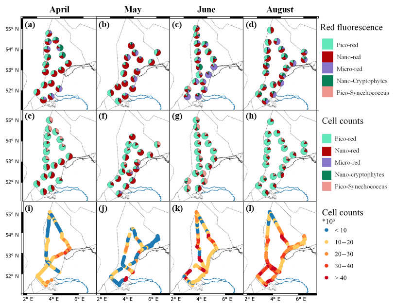
Figure 3Relative phytoplankton community composition using FCM-derived total red fluorescence (a–d) and cell numbers (e–h) in April, May, June, and August (from left to right). The groups are clustered according to Table 2. Figure made with QGIS v2.14.2 using EEZ zone data from the Flanders Marine Institute (2018).
3.2 Phytoplankton abundance and fluorescence
Before the ANCOVA, natural logarithm transformations were required to correct for the inhomogeneity of the residuals and unequal variances between months. Both the FRRf F0 (p<0.01, adjusted R2=0.66) and FCM total red fluorescence (p<0.01, adjusted R2=0.90) provided significant predictors of HPLC-derived Chl a concentration (Fig. 2). The ANCOVA with the FRRf-derived F0 as a Chl a predictor revealed that the slope did not differ per month, but the intercept did (p<0.01). The ANCOVA with the FCM-derived TFLR as a Chl a predictor resulted not only in a significant difference of the Chl a concentration per month (p<0.01) but also in a significantly different slope (p<0.05), suggesting that other predictors that differ per month were influencing the fluorescence per Chl a molecule (Fig. 2).
3.3 Phytoplankton community composition
In April the northern part of the Dutch North Sea was numerically dominated by picoplankton, whereas the southern part and the northern coastal area of the Dutch EEZ were numerically dominated by nanophytoplankton. The taxa with a high phycoerythrin content (Synechococcus and Cryptophyceae) made up only a small proportion of the total phytoplankton community in April (generally less than 10 %) and were most abundant in the northern part of the Dutch North Sea (Fig. 3e). Microphytoplankton always represented less than 3 % of the total community. The highest microphytoplankton abundance was found close to the Dutch delta and along the Noordwijk transect. The spatial patterns of the phytoplankton community in May were smaller in comparison to April (Fig. 3b, f, j). Picophytoplankton abundance was highest offshore (60 %–80 %), whereas the highest percentage of nanophytoplankton was observed north of Terschelling 100 and in the coastal zone (Fig. 3f). Between May and June the community composition shifted and phytoplankton cell numbers increased. Both groups of picophytoplankton (Synechococcus and pico-red) increase in relative abundance between May and June, while the nanophytoplankton shows a strong decrease (Fig. 3). The highest abundance of picophytoplankton was observed offshore. The microphytoplankton was the largest contributor to red fluorescence in the coastal region, although this group does not increase in relative abundance in comparison to May (Fig. 3). In August the picophytoplankton dominated the phytoplankton communities, with an average contribution to total cell numbers of over 80 %, and only slightly lower values were observed (but still >70 %) along the southern Dutch coast, where the abundance of nanophytoplankton was higher. Microphytoplankton were hardly observed, although with their high red fluorescence per cell, they contributed to up to half of the total red fluorescence in coastal regions.
3.4 Photophysiology
In April, the photophysiology of the phytoplankton communities in the Dutch North Sea showed low variability. The Fv∕Fm values stayed above 0.5 in northern regions and above 0.4 in southern regions (Fig. 4a). The σPSII stayed in a narrow range between 2.5 and 4 nm2 PSII−1 (Fig. 4e). The Ek in April showed more variability in comparison to the Fv∕Fm and σPSII. In the coastal zone, the Ek was lower off the coast of Walcheren and higher off the coast of Noordwijk. In offshore regions, no clear spatial patterns were present (Fig. 4i). In May the photophysiological parameters of the phytoplankton communities in the Dutch North Sea were strongly heterogeneous with only smaller-scale spatial patterns (Fig. 4b, f, j). Fv∕Fm was in general lower in May (0.1–0.5) than in April (>0.4) across most of the Dutch EEZ (Fig. 4b). In May the σPSII was high (average 5.9 nm2 PSII−1) across the Dutch North Sea, except near the coast of Noordwijk (Fig. 4f). In the same region, the Ek was high (>450 µmol photons m−2 s−1), but this concurrent signal (high Ek, low σPSII) did not occur in other regions of the Dutch North Sea. The Ek across the Dutch North Sea in May was heterogeneous without large-scale spatial patterns. In June the spatial patterns in the photophysiology of the phytoplankton in the Dutch North Sea were less heterogeneous and larger mesoscale spatial patterns could be identified. The Fv∕Fm values recovered in comparison to May to above 0.4 in the coastal zone but not in offshore regions in the southern North Sea. The Fv∕Fm of the southern offshore phytoplankton, between Walcheren 70 and Noordwijk 70 (Fig. 1), remained low (<0.2; Fig. 4c). The σPSII was lower in comparison to May across the Dutch North Sea, apart from the southern offshore region (Fig. 4g). In a small region around Noordwijk 70, the phytoplankton community had a particularly low σPSII (<2.5 nm2 PSII−1), which did not present itself in anomalies in the other photophysiological parameters. The Ek in June was low in the northern coastal zone and higher in offshore regions (Fig. 4k). In August the Fv∕Fm recovered across the Dutch North Sea (Fig. 4d). The σPSII was high in the northern offshore region and comparable to June in the rest of the Dutch North Sea (Fig. 4h). In August the regions of the Noordwijk coast and the coast of the Wadden Islands were sampled twice at two different times of the day. This repeated measurement resulted in a higher Ek, suggesting diurnal variability. To further investigate daily patterns standardized, daily anomalies (Z scores) were calculated. These show a clear diurnal trend in photosynthetic activity (Fig. 5). The Fv∕Fm was lowest during the middle of the day, while Ek, σPSII, and 1∕τ peaked during the middle of the day. As Ek was strongly correlated with Pmax (Fig. S2), a clear diurnal pattern was also present in the photosynthetic electron transport rate.
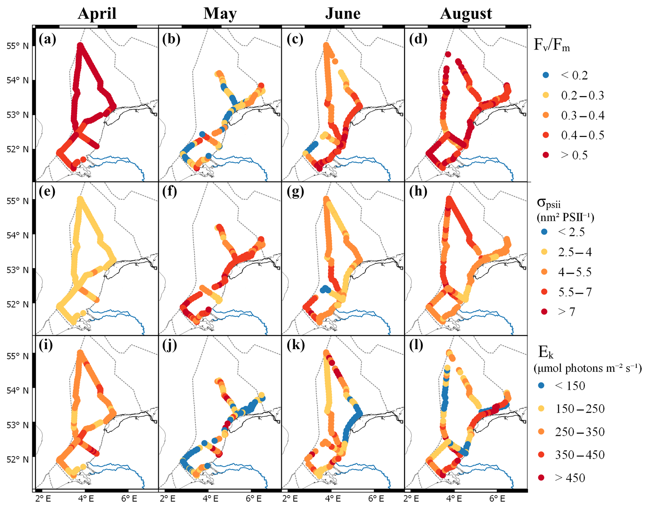
Figure 4Maps of the photophysiological parameters Fv∕Fm (a–d), σPSII (e–h; nm2 PSII−1) and Ek (i–l; µmol photons m−2 s−1) per month (from left to right: April, May, June, and August). For more details on the location see Fig. 1. Figure made with QGIS v2.14.2 using EEZ zone data from the Flanders Marine Institute (2018).
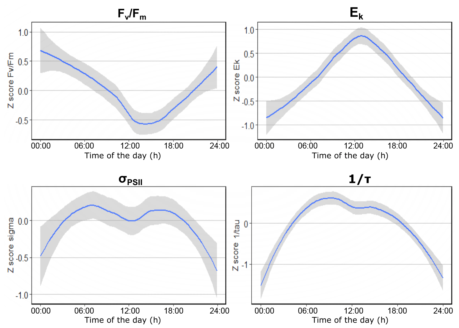
Figure 5Standardized daily anomalies (z scores) of Fv∕Fm, Ek, σPSII, and 1∕τ showing the diurnal trends in photophysiological data. On the x axis is the time of the day and on the y axis is the z score. Figure made using the ggplot2 package in R (Wickham, 2009).
3.5 Gross primary productivity
Gross primary productivity ranged from 0.35 µg C L−1 h−1 in June to 602 µg C L−1 h−1 in the coastal zone in May (Fig. 6). The average GPP was highest in April and lowest in August. Monthly averages ranged from 116±59 µg C L−1 h−1 in April to 8.7±8.3 µg C L−1 h−1 in August, although these averages are not completely comparable due to different ship routes per month (Fig. 6). In April, spatial heterogeneity in GPP was low. The highest rates in April were measured offshore (>250 µg C L−1 h−1) and in the coastal regions close to the Wadden Islands (Terschelling 10 in Fig. 1). In May, the GPP was heterogeneous without a clear spatial pattern. Most production rates stayed below 30 µg C L−1 h−1, with local GPP peak rates over 600 µg C L−1 h−1 in the southern coastal zone. In June, the GPP was on average lower than in May and showed more large-scale spatial patterning. The highest values in June were observed (30–40 µg C L−1 h−1) northwest of Noordwijk. In August, GPP was low throughout the Dutch North Sea, with the majority of productivity rates staying below 10 µg C L−1 h−1. In the southern coastal zone, slightly higher rates were found, reaching up to 50 µg C L−1 h−1.
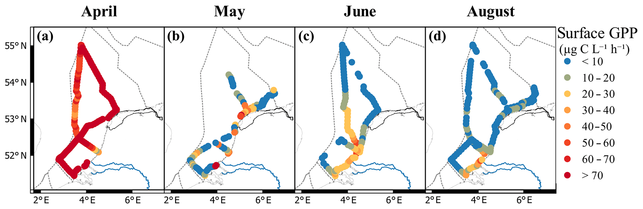
Figure 6Gross primary productivity of the surface (a–d; µg C L−1 h1) per month (a–d: April, May, June, and August). Colors represent rates; blue is low and red is high (see legend). Figure made with QGIS v2.14.2 using EEZ zone data from the Flanders Marine Institute (2018).
3.6 Spatial clustering
Strong collinearity between measured parameters was present. For spatial clustering these were removed based on the variable inflation factor (VIF >6; see the Supplement for pair plots), which resulted in the removal of the photophysiological parameters Pmax, α, aLHII, nPSII, the FCM parameter of the total red fluorescence, and the GPP. From the five defined phytoplankton groups (Table 2), the nano-crypto group was not used in the clustering because of collinearity (VIF >6). The remaining variables were the abundance of the remaining four FCM-defined phytoplankton groups (pico-red, pico-synecho, nano-red, and micro-red), the total O ∕ R ratio, and five photophysiological parameters (Fv∕Fm, σPSII, 1∕τ, RCII, and Ek). For an overview of the collinearity between variables, see the pair plots in the Supplement.
Spectral cluster analysis resulted in the identification of two to four clusters in each cruise. Most of these clusters were spatially separated and can therefore be considered regions with distinct phytoplankton communities (Fig. 7). In April, the clustering resulted in three clusters with a clear spatial pattern. In the PCA, the variables that contributed most to the first principal component were all biomass related: RCII and aLHII, related to the photosynthetic capacity per reaction center and per volume, and the abundance of the nano-red group. The second principal component has photosynthetic parameters as two main contributors (σPSII and 1∕τ; 51.5 %). Cluster 1 covered most of the northern part of the Dutch North Sea and a small part of the Noordwijk transect to the coast. The bi-plot of the PCA showed that the first cluster was negatively correlated with the main contributors of PC1 (RCII and aLHII; Fig. 7), so this region consisted of a phytoplankton community with lower photosynthetic capacity per liter. The coastal region was separated into two clusters, 2 and 3, with overlapping confidence ellipses (Fig. 7). The confidence interval of cluster 2 is larger than cluster 3, suggesting that the phytoplankton community in cluster 2 was more heterogeneous. Both clusters are positively correlated with the main contributors to PC1 (RCII and aLHII), meaning these clusters consist of a community with higher photosynthetic capacity per volume. In May, the cluster analysis resulted in four different clusters but without a well-defined spatial pattern. The PCA bi-plots showed that the confidence interval of cluster 5 overlaps most of the other clusters, indicating that this cluster has weak support. Ek was negatively correlated with cluster 4 and σPSII, suggesting that cluster 4 contained low-light-acclimated algae. In contrast, in June only two clusters with a distinct separation between coastal and offshore phytoplankton communities were found. The PCA showed that the offshore phytoplankton community consisted of a diverse phytoplankton community, while the coastal phytoplankton community had high Fv∕Fm, aLHII, and RCII. In August not all clusters were spatially separated (Fig. 7). Different clusters were appointed to the same region visited within a 2 d time span twice: in the northeastern coastal region and at the transect of Noordwijk. Both times, cluster 11 is one of the overlapping spatial clusters. Cluster 11 corresponds to only nighttime sampling periods and was defined by low Ek and low 1∕τ, indicative of a low-light-acclimated phytoplankton community. This suggests that cluster 11 was a temporal cluster instead of a spatial cluster. To test this we repeated the analysis for the month of August but only including the measurements performed within an 8 h timeframe around noon (12:00 ± 4 h LT; Fig. S4). In this timeframe, the southern coastal zone was distinct from the rest of the Dutch North Sea and corresponded to cluster 10 in the analysis of the complete dataset (Fig. 7d), so this cluster was defined by spatial variability. Clusters 12 and 13 were grouped together in the 12:00 ± 4 h timeframe as cluster 1. Cluster 11 was not recognized as a cluster within the 12:00 ± 4 h timeframe, so it indeed seemed controlled by temporal rather than spatial variability.
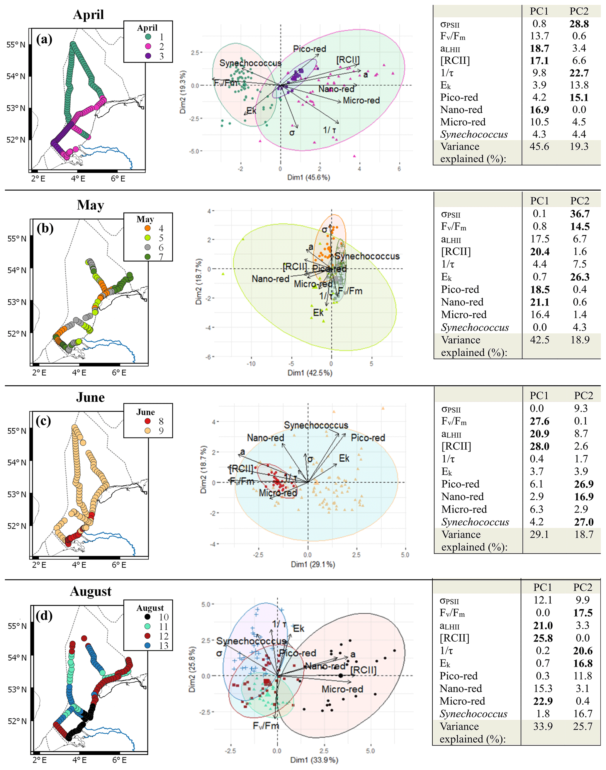
Figure 7Overview of the spectral cluster analysis based on the non-collinear phytoplankton parameters (FCM: pico-red, nano-red, micro-red, Synechococcus; FRRf: σPSII, Fv∕Fm, aLHII, 1∕τ, Ek) separated per month (a to d: April, May, June, and August). On the left the clusters are visualized on maps and in the middle are the bi-plots of the PCA of the data with confidence ellipses per cluster (confidence 95 %). In all graphics clusters are visualized by different colors as shown in the legend inset. For the confidence ellipses the border lines (and not the fill) correspond to the clusters. In the bi-plot overlapping confidence ellipses suggest a high similarity between groups, while the size of the ellipse is a measure of variability within the group. On the right is the PCA table with contributions in percent of the different variables; in bold are the three variables that contribute most to the principal component. Maps were made with QGIS v2.14.2 using EEZ zone data from the Flanders Marine Institute (2018). The PCA visualization was done in R using the supplemental R package factoextra (Kassambra and Mundt, 2017).
The objective of this study was to evaluate the added value of FRR fluorometry and flow cytometry for monitoring purposes. During four cruises spread over 5 months, a wide variety of environmental conditions and phytoplankton community states were sampled. Here, these data are used to evaluate the potential of this approach to be developed as a novel method to improve existing monitoring (OSPAR, MSFD).
Biomass is an important parameter to understand the role of phytoplankton in the ecosystem and biogeochemical cycles. Its direct measurement using high-resolution methods is challenging. Chlorophyll a concentration is often used as an estimate for biomass, although the carbon : Chl a ratio is dependent on abiotic conditions and species-specific phenotypic plasticity, and chlorophyll a is therefore not directly related to biomass (Flynn, 1991, 2005; Geider et al., 1997; Alvarez-Fernandez and Riegman, 2014; Halsey and Jones, 2015). In this study, chlorophyll concentrations are estimated by red fluorescence, which results in a good fit for both the FRRf (adjusted R2=0.66) and the FCM (adjusted R2=0.90). The impact of abiotic conditions on fluorescence as a predictor for chlorophyll a content was tested by comparing the relationship in the different months. Only the flow cytometer data were significantly affected by environmental conditions. The different environmental conditions per month did not affect the regression line of the FRRf data. Since the two instruments differ in optics as well as measurement setup (measurements per cell vs. bulk), differences are not surprising. The different measurement setup, with the flow cytometer measuring the fluorescence per particle, while the FRRf does a measurement of the bulk sample, might blur the effect of environmental conditions. In a bulk measurement, other particles in solution scatter the excitation and emission photons, plus the emitted fluorescence of the phytoplankton is subject to reabsorption, especially at higher biomass densities. Yet, the difference most affected by environmental conditions is the fluorescent state of the photosystems. The strong laser of the flow cytometer can only measure the maximum fluorescence (Fm), which is a parameter more prone to quenching than the minimum fluorescence measured by the FRRf. The lower sensitivity to environmental conditions implies that the FRRf is better suited to estimate chlorophyll a concentration in comparison to the FCM. Other studies that estimate chlorophyll a concentrations with FCM and fluorometers also find better fits using bulk measurements by a fluorometer in comparison to flow cytometric measurements per cell (Thyssen et al., 2015; Marrec et al., 2018). An alternative to the controversial use of chlorophyll a as an estimate for biomass is the derivation of biomass or biovolume from cell counts. This requires assumptions on cell size, cell shape, and carbon content per biovolume (Tarran et al., 2006). Another alternative is to derive biovolume from the scattering properties of the cell using a pulse-shape recording flow cytometer, as used in this study. This relationship appears to be taxon specific (Machteld Rijkeboer, personal communication, 2018) and needs to be further explored by comparison of calculated biovolume (based on image-in-flow pictures) and the flow cytometric properties of the cell. The FRRf offers the possibility to circumvent the use of phytoplankton biomass as a necessary parameter to estimate primary productivity altogether by estimating the number of photosystem II reaction centers or total absorption by the PSII concentration (i.e., aLHII; Oxborough et al., 2012). As long as there is no uncontroversial method to derive phytoplankton biomass, the calculation of multiple parameters and critical evaluation remain necessary.
The FCM was able to visualize the spatial variability of the phytoplankton community in the Dutch North Sea. The typical spring bloom was partly captured during the cruise in April, with high total fluorescence and high relative abundance of microphytoplankton and nanophytoplankton in comparison to other months. In contrast, in August the community was dominated by picophytoplankton with only sporadic observations of microphytoplankton. In addition, spatial variability in size distribution was clearly visible as a stronger presence of microphytoplankton in coastal regions than offshore. Microphytoplankton are a better food source for higher trophic levels than picophytoplankton. Picophytoplankton is part of the microbial food web, with less trophic efficiency and a low contribution to carbon export (Azam et al., 1983; Finkel et al., 2010). The shift from nanophytoplankton-dominated communities in April to picophytoplankton-dominated communities in August therefore indicates that over the year the tropic efficiency and carbon export decrease. These spatial and temporal changes are yearly phenomena, influenced by the strong seasonal dynamics in the Dutch North Sea that affect the spatial distribution and community composition of the phytoplankton community (Baretta-Bekker et al., 2009; Brandsma et al., 2012). It is important to monitor interannual variability over the years to monitor changes in biogeochemical cycles and the carrying capacity of the ecosystem. To increase the informational value of the flow cytometry data beyond size, the FCM clusters would need to reflect taxonomic or functionally relevant groups. Interesting groups include calcifiers, silicifiers, DMS producers (such as Phaeocystis), or nitrogen fixers (le Quéré et al., 2005). The lack of identification of distinct clusters has made this impossible so far, although some species are recognizable such as Phaeocystis sp. (Rijkeboer, unpublished). Marrec et al. (2018) manually separated up to 10 phytoplankton groups from the data of the CytoSense flow cytometer. Yet, most of these groups comprise many taxonomic genera, which, apart from the size or pigment composition, hinders further interpretation of their role in the ecosystem or biogeochemical cycles. However, the distinction between different pigment groups can provide useful information on food web functioning. Chlorophyll c containing algae (Chromista) contain long-chained essential fatty acids like docosahexaenoic acid (DHA) and eicosapentaenoic acid (EPA), which are lacking in green algae (some Prasinophyceae excepted) and cyanobacteria (Dijkman and Kromkamp, 2006). Thus, information about food quality can be obtained from FCM. For the detection of nuisance phytoplankton, distinct clusters are lacking. Yet, toxicity in phytoplankton can differ even between strains within one species, so finding a distinct cluster by flow cytometry is challenging (Tillman and Rick, 2003). However, the identification of “suspicious” clusters with potential toxic species could be helpful. These suspicious clusters can flag sampling points to be further inspected by a specialist using microscopy.
Monitoring of the photophysiology of phytoplankton by FRR fluorometry can supplement flow cytometry measurements. For instance, the hypothesized spring bloom detected by flow cytometer in April is confirmed by photophysiological parameters; photophysiology was uniform and primary productivity high. Between April and May, the efficiency of PSII (Fv∕Fm; Fig. 4) decreased throughout the Dutch North Sea. A decreasing Fv∕Fm is generally associated with limiting nutrient conditions or other abiotic conditions but can also reflect a change in community composition stressors (Suggett et al., 2009b; Kolber et al., 1988; Kolber and Falkowski, 1993; Beardall et al., 2001; Ly et al., 2014). Photophysiological parameters vary per taxonomic group; smaller taxa typically have lower Fv∕Fm values and higher σPSII values (Kolber et al., 1988; Suggett et al., 2009b). No major shift in community composition was identified by flow cytometry between April and May. This suggests that an abiotic stressor, such as the nutrient-limiting conditions in a large part of the Dutch North Sea, instead of the community composition was driving the decrease in the efficiency of PSII. In contrast, the recovery of the Fv∕Fm between May and June coincided with a shift in community composition. In May the phytoplankton communities were mostly nanophytoplankton dominated, while in June the communities were dominated by picophytoplankton (offshore) and microphytoplankton (coastal). So, although recovery of the Fv∕Fm can also occur as an adaptation of phytoplankton to nutrient-limiting conditions (Kruskopf and Flynn, 2005), it seems that the shift in community composition was the major driver for the recovery of the Fv∕Fm between May and June. These findings are a good example of how concurrent measurements by flow cytometry and fast repetition rate fluorometry can supplement improved ecosystem understanding.
When including photophysiology (or photophysiology-based GPP estimates) in a monitoring program, it is critical to consider methodological constraints (Hughes et al., 2018). For instance, at low phytoplankton abundance, the fluorescence signal becomes too noisy for the calculation of parameters. Moreover, blank correction is essential for retrieving accurate FRRf data (Cullen and Davis, 2003). FRRf measurements are affected by the interference of colored dissolved matter, which can lead to underestimation or overestimation of some parameters (like Fv∕Fm; Cullen and Davis, 2003). Blank correction is a manual measurement and should be done regularly, at least when abiotic conditions change (Hughes et al., 2018). For monitoring purposes, it is important to take into account diurnal variability. Diurnal trends make extrapolation to daily rates challenging. Most of the photophysiological parameters we measured showed diurnal trends (Fig. 5). The diurnal trend is dictated by the phytoplankton cell cycle, a circadian oscillator, and photophysiological response to varying irradiance (Suzuki and Johnson, 2001; Cohen and Golden, 2015; Schuback et al., 2016). Phytoplankton use photophysiological plasticity to minimize photodamage and optimize growth under fluctuating irradiance (Schuback et al., 2016; Behrenfeld et al., 2002). The electron requirement for carbon fixation is also subject to diurnal variation (Schuback et al., 2016; Lawrenz et al., 2013; Raateoja, 2004). To interpret spatial variability separately from temporal variability and to provide a more reliable estimate of gross primary productivity, Schuback et al. (2016) suggest a correction with normalized Stern–Volmer quenching (NPQNSV). This approach needs further research, for example by using a Lagrangian approach whereby the photosynthetic activity of the same population is followed during the day. Until a reliable correction method has been established, a monitoring program including photophysiology should account for diurnal variability, for instance by using only measurements collected in a certain timeframe or from buoys. Despite the limitations of GPP estimates by variable fluorescence, our results clearly show large spatial variability in gross primary production that is not explained by diurnal variability. This spatial heterogeneity is not fully captured by sampling at standard low-resolution monitoring stations, showing the added value of our approach.
Phytoplankton biomass does not necessarily reflect primary productivity, as high grazing pressure can keep biomass low while production is high. This is clearly visualized by the lack of resemblance between patterns in cell numbers (Fig. 3a–d) and gross primary productivity (Fig. 6). Gross primary productivity estimates by FRR fluorometry are based on measurements of the first step of photosynthesis: the efficiency at which photons are captured and electrons transferred. However, to interpret gross primary productivity in an ecologically or biogeochemically meaningful way, the FRR units of electrons per unit time need to be converted to carbon units. In general, gross photosynthesis correlates well with photosynthetic oxygen evolution (Suggett et al., 2003), and multiple studies have shown a good correlation between 14C-derived estimates of primary productivity and FRRf-derived estimates using a constant conversion factor (Melrose et al., 2006; Kromkamp et al., 2008). However, in reality, this parameter is not a constant as along the pathway from electron to carbon atom electrons are consumed by other cell processes (Flameling and Kromkamp, 1998; Halsey and Jones, 2015; Schuback et al., 2016). As the cell processes from photon absorbance to carbon assimilation are known to vary with abiotic conditions, we expect that the identification of biogeographic regions can aid in predicting regional Φe,C (Lawrenz et al., 2013). Calibration with other methods, such as concurrent 14C of 13C incubations, could help us to better understand the processes from electron excitation to carbon fixation. However, these methods introduce other uncertainties; they measure a type of productivity between net and gross primary productivity, depending on the incubation time and growth rate of the phytoplankton (Halsey and Jones, 2015). For now, a reliable GPP estimate in carbon units from FRR fluorometry requires more research, and estimates provide relative rather than qualitative values. Despite its limitations, the ability to study live phytoplankton rates without long-term incubation effects makes the method promising. Additionally, the high sampling resolution allows for the identification of extra sampling points based on real-time projections, opening up early warning methodologies. For example, in the April cruise both Noordwijk 70 and Terschelling 235 km show high gross primary productivity, but between them both high and low productivity rates occur, which are not detected with the current sampling program (Fig. 6). Extrapolation of surface measurements to water column estimates is required to assess the carrying capacity of the ecosystem and the contributions to biogeochemical cycles. Surface water measurements are only a good reflection of the water column when mixed layer depth is deeper than the euphotic zone. Stratification or a mixed layer depth shallower than the euphotic zone can result in subsurface chlorophyll maximum layers and significantly different phytoplankton communities (Latasa et al., 2017). Only frequent CTD casts equipped with PAR sensors can determine the vertical heterogeneity, mixed layer depth, and light extinction in the water column.
High-resolution methods such as the FRRf and the flow cytometer result in a multitude of parameters. Cluster methods can be helpful in bringing together these parameters for interpretation. The spectral clustering method used in this study was originally designed to detect phytoplankton blooms and understanding the involved dynamics (Rousseeuw et al., 2015; Lefebvre and Poisson-Caillault, 2019). This spectral cluster analysis of parameters from the FRRf and the flow cytometer allowed for the identification of distinct phytoplankton communities or biogeographic regions that differed per cruise. A clear distinction between phytoplankton communities of the coastal zone and offshore regions could be made in all months, except May. In two cruises, in April and June, it was indeed possible to identify regions with distinct phytoplankton communities. During the cruise in May, the clustering did not result in clear mesoscale patterns but was heterogeneous over the whole Dutch North Sea. Unfortunately, the model was not able to visualize all spatial heterogeneity. For instance, in April off the coast of Terschelling a distinct community with a high abundance of phycoerythrin-containing taxa did not result in a separate cluster. Additionally, temporal variation (i.e., day–night differences) interfered with the spatial clustering in August. So, although such models are useful for visualization and following changes in spatial heterogeneity, input and output need to be critically evaluated before implementation in monitoring programs. To test whether the differences between months result from seasonal variation or other factors, results over multiple years and additional seasonal cruises need to be obtained to better characterize the heterogeneity of the phytoplankton community structure.
The purpose of a phytoplankton monitoring program is to monitor the presence of functional types of phytoplankton, including the harmful taxa, the carrying capacity of the ecosystem, and changes in biogeochemical cycling. The objective of this study was to evaluate the use of FRR fluorometry and flow cytometry for such monitoring purposes. The four conducted cruises spread over 5 months offered a wide variety of environmental conditions and phytoplankton community states, which the utilized methods were able to visualize. Inclusion of high-resolution methods in monitoring programs allows for analysis of finer-scale events. Furthermore, it allows for analysis of living phytoplankton and is thereby able to measure rates and avoid the effects of preservation and storage of samples. Another advantage is that high-resolution methods allow for easier comparison between countries once common protocols are established. Nevertheless, low-resolution methods remain a necessity for more detailed taxonomic analysis, extrapolation over the entire water column, and to calibrate and correct for blanks. Data analysis is a challenge when implementing high-resolution methods, whereby cluster methods could simplify and standardize analysis. The cluster analysis of flow cytometric data has potential for improvement to increase the informative value of the method. The identification of phytoplankton clusters with a functional quality, such as nitrogen fixers, calcifiers, DMS producers, or clusters with high food quality, would particularly be helpful for the interpretation of ecosystem dynamics and biogeochemical fluxes. Regarding the FRRf, the main challenge is converting the electron transport rate to gross primary productivity in carbon units. Further research on these topics would benefit the implementation of these methods in monitoring protocols. Furthermore, it is important to account for diurnal patterns in monitoring setup to be able to distinguish between diurnal and spatial variability. Possibly, diurnal variability could be modeled, but more studies with a Lagrangian-based approach are needed for a better understanding of the impact of diurnal variability in the data. The combination of high-resolution in situ methods with remote sensing has the potential to further increase the spatial and temporal scale. Estimating biological parameters using remote sensing is challenging, especially in turbid waters (Gohin et al., 2005; van der Woerd et al., 2008). Therefore, in vivo measurements are required to calibrate remote-sensing-based models, and we suggest that automated flow cytometry and production measurements based on FRRf methodology can fulfill this role. Overall, our proposed high-resolution measurement setup has the potential to improve phytoplankton monitoring by supplementing existing low-resolution monitoring programs.
Data are publically available at 4TU.ResearchData: https://doi.org/10.4121/uuid:84406786-219d-4f33-a60a-a0f5301032d0 (Aardema et al., 2019).
The supplement related to this article is available online at: https://doi.org/10.5194/os-15-1267-2019-supplement.
HMA, MR, JCK, and AV designed the measurement setup. HMA, MR, and JCK collected the data. HMA, MR, AL, and JCK contributed to data processing. HMA and JCK prepared the figures and tables. HMA, MR, JCK, AL, and AV prepared the paper.
The authors declare that they have no conflict of interest.
This article is part of the special issue “Coastal marine infrastructure in support of monitoring, science, and policy strategies”. It is not associated with a conference.
We want to thank the captain and crew of the RV Zirfaea and the shipboard Eurofins employees for their hospitality and great help during the cruises. We thank Annette Wielemaker for assistance with the GIS maps of primary production, René Geertsema for assistance with the flow cytometry data analysis, and Ralf Schiebel for useful comments on the paper. Furthermore, we would like to thank the Rijkswaterstaat laboratory for conducting the nutrient and chlorophyll measurements and Rijkswaterstaat for the opportunity to perform measurements alongside the regular monitoring program.
This research has been supported by the European Union's Horizon 2020 research and innovation program
(grant no. 654410, JERICO-NEXT).
The article processing charges for this open-access
publication
were covered by the Max Planck Society.
This paper was edited by Antoine Gremare and reviewed by two anonymous referees.
Aardema, H. M., Rijkeboer, M., Levebvre, A., Veen, A., and Kromkamp, J. C.: Data presented in the paper “High-resolution underway measurements of phytoplankton photosynthesis and abundance as innovative addition to water quality monitoring programs”, https://doi.org/10.4121/uuid:84406786-219d-4f33-a60a-a0f5301032d0, 2019.
Alvarez-Fernandez, S. and Riegman, R.: Chlorophyll in North Sea coastal and offshore waters does not reflect long term trends of phytoplankton biomass, J. Sea Res., 91, 35–44, https://doi.org/10.1016/j.seares.2014.04.005, 2014.
Azam, F., Fenchel, T., Field, J., Gray, J., Meyer-Reil, L., and Thingstad, F.: The Ecological Role of Water-Column Microbes in the Sea, Mar. Ecol. Prog. Ser., 10, 25–263, 1983.
Baretta-Bekker, J. G., Baretta, J. W., Latuhihin, M. J., Desmit, X., and Prins, T. C.: Description of the long-term (1991–2005) temporal and spatial distribution of phytoplankton carbon biomass in the Dutch North Sea, J. Sea Res., 61, 50–59. https://doi.org/10.1016/j.seares.2008.10.007, 2009.
Beardall, J., Berman, T., Heraud, P., Kadiri, M. O., Light, B. R., Patterson, G., Roberts, S., Sulzberger, B., Sahan, E., Uehlinger, U., and Wood, B.: A comparison of methods for detection of phosphate limitation in microalgae, Aquat. Sci., 63, 107–121, 2001.
Behrenfeld, M. J., Maranon, E., Siegel, D. A., and Hooker, S. B.: Photoacclimation and nutrient-based model of light-saturated photosynthesis for quantifying oceanic primary production, Mar. Ecol. Prog. Ser., 228, 103–117, 2002.
Behrenfeld, M. J., O'Malley, R. T., Siegel, D. A., McClain, C. R., Sarmiento, J. L., Feldman, G. C., Milligan, A. J., Falkowski, P. G., Letelier, R. M., and Boss, E. S.: Climate-driven trends in contemporary ocean productivity, Nature, 444, 752–755, https://doi.org/10.1038/nature05317, 2006.
Brandsma, J., Hopmans, E. C., Philippart, C. J. M., Veldhuis, M. J. W., Schouten, S., and Sinninghe Damsté, J. S.: Low temporal variation in the intact polar lipid composition of North Sea coastal marine water reveals limited chemotaxonomic value, Biogeosciences, 9, 1073–1084, https://doi.org/10.5194/bg-9-1073-2012, 2012.
Burson, A., Stomp, M., Akil, L., Brussaard, C. P. D., and Huisman, J.: Unbalanced reduction of nutrient loads has created an offshore gradient from phosphorus to nitrogen limitation in the North Sea, Limnol. Oceanogr., 61, 869–888, https://doi.org/10.1002/lno.10257, 2016.
Capuzzo, E., Stephens, D., Silva, T., Barry, J., and Forster, R. M.: Decrease in water clarity of the southern and central North Sea during the 20th century, Glob. Change Biol., 21, 2206–2214, https://doi.org/10.1111/gcb.12854, 2015.
Capuzzo, E., Lynam, C. P., Barry, J., Stephens, D., Forster, R. M., Greenwood, N., McQuatters-Gollop, A., Silva, T., van Leeuwen, S. M., and Engelhard, G. H.: A decline in primary production in the North Sea over 25 years, associated with reductions in zooplankton abundance and fish stock recruitment, Glob. Change Biol., 0, 1–13, https://doi.org/10.1111/gcb.13916, 2017.
Cloern, J. E., Foster, S. Q., and Kleckner, A. E.: Phytoplankton primary production in the world's estuarine-coastal ecosystems, Biogeosciences, 11, 2477–2501, https://doi.org/10.5194/bg-11-2477-2014, 2014.
Cohen, S. E. and Golden, S. S.: Circadian Rhythms in Cyanobacteria, Microbiol. Mol. Biol. R., 79, 373–385, https://doi.org/10.1128/MMBR.00036-15, 2015.
Cullen, J. J. and Davis, R. F.: The blank can make a big difference in oceanographic measurements, Limnol. Oceanogr. Bulletin, 12, 29–35, 2003.
Dijkman, N. A. and Kromkamp, J. C. Phospholipid-derived fatty acids as chemotaxonomic markers for phytoplankton: application for inferring phytoplankton composition, Mar. Ecol. Progr. Ser., 424, 113–125, 2006.
Falkowski, P. G.: Biogeochemical Controls and Feedbacks on Ocean Primary Production, Science, 281, 200–206, https://doi.org/10.1126/science.281.5374.200, 1998.
Finkel, Z. V., Beardall, J., Flynn, K. J., Quigg, A., Rees, T. A. V., and Raven, J. A.: Phytoplankton in a changing world: cell size and elemental stoichiometry, J. Plankton Res., 32, 119–137, https://doi.org/10.1093/plankt/fbp098, 2010.
Flameling, I. A. and Kromkamp, J. C.: Light dependence of quantum yields for PSII charge separation and oxygen evolution in eukaryotic algae, Limnol. Oceanogr., 43, 284–297, 1998.
Flanders Marine Institute: Maritime Boundaries Geodatabase: Maritime Boundaries and Exclusive Economic Zones (200NM), version 10, https://doi.org/10.14284/312, 2018.
Flynn, K. J.: Algal carbon-nitrogen metabolism: a biochemical basis for modelling the interactions between nitrate and ammonium uptake, J. Plankton. Res., 13, 373–387, 1991.
Flynn, K. J.: Modelling marine phytoplankton growth under eutrophic conditions, J. Sea Res., 54, 92–103, 2005.
Geider, R. J., MacIntyre, H. L., and Kana, T. M.: Dynamic model of phytoplankton growth and acclimation: responses of the balanced growth rate and the chlorophyll a : carbon ratio to light, nutrient-limitation and temperature, Mar. Ecol. Prog. Ser., 148, 187–200, 1997.
Gohin, F., Loyer, S., Lunven, M., Labry, C., Froidefond, J.-M., Delmas, D., Huret, M., and Herbland. A.: Satellite-derived parameters for biological modelling in coastal waters: Illustration over the eastern continental shelf of the Bay of Biscay, Remote Sens. Environ., 95, 29–46, 2005.
Goss, R., Ann Pinto, E., Wilhelm, C., and Richter, M.: The importance of a highly active and ΔpH-regulated diatoxanthin epoxidase for the regulation of the PS II antenna function in diadinoxanthin cycle containing algae, J. Plant Physiol., 163, 1008–1021, https://doi.org/10.1016/j.jplph.2005.09.008, 2006.
Halsey, K. H. and Jones, B. M.: Phytoplankton Strategies for Photosynthetic Energy Allocation, Annu. Rev. Mar. Sci., 7, 265–97, https://doi.org/10.1146/annurev-marine-010814-015813, 2015.
Hughes, D. J., Campbell, D. A., Doblin, M. A., Kromkamp, J. C., Lawrenz, E., Moore, C. M., Oxborough, K., Prášil, O., Ralph, P. J., Alvarez, M. F., and Suggett, D. J.: Roadmaps and Detours: Active Chlorophyll a Assessments of Primary Productivity Across Marine and Freshwater Systems, Environ. Sci. Technol., 52, 12039–12054, https://doi.org/10.1021/acs.est.8b03488, 2018.
Kassambara, A. and Mundt, F.: factoextra: Extract and Visualize the Results of Multivariate Data Analyses, R package version 1.0.5, available at: https://CRAN.R-project.org/package=factoextra (last access: 1 February 2018), 2017.
Kolber, Z. and Falkowski, P. G.: Use of active fluorescence to estimate phytoplankton photosynthesis in situ, Limnol. Oceanogr., 38, 1646–1665, 1993.
Kolber, Z., Zehr, J., and Falkowski, P. G.: Effects of growth irradiance and nitrogen limitation on photosynthetic energy conversion in photosystem II, Plant Physiol., 88, 923–929, 1988.
Kolber, Z. S., Prášil, O., and Falkowski, P. G.: Measurements of variable chlorophyll fluorescence using fast repetition rate techniques: Defining methodology and experimental protocols, BBA-Bioenergetics, 1367, 88–106, https://doi.org/10.1016/S0005-2728(98)00135-2, 1998.
Kromkamp, J. C. and Forster, R. M.: The use of variable fluorescence measurements in aquatic ecosystems: differences between multiple and single turnover measuring protocols and suggested terminology, Eur. J. Phycol., 38, 103–112, https://doi.org/10.1080/0967026031000094094, 2003.
Kromkamp, J. C. and Van Engeland, T.: Changes in phytoplankton biomass in the western Scheldt estuary during the period 1978–2006, Estuaries Coasts, 33, 270–285, https://doi.org/10.1007/s12237-009-9215-3, 2010.
Kromkamp, J. C., Dijkman, N. A., Peene, J., Simis, S. G. H., and Gons, H. J.: Estimating phytoplankton primary production in Lake IJsselmeer (the Netherlands) using variable fluorescence (PAM-FRRF) and C-uptake techniques Estimating phytoplankton primary production in Lake IJsselmeer (the Netherlands) using variable fluoresce, Eur. J. Phycol., 43, 327–344, https://doi.org/10.1080/09670260802080895, 2008.
Kruskopf, M. and Flynn, K. J.: Chlorophyll content and fluorescence responses cannot be used to gauge reliably phytoplankton biomass, nutrient status or growth rate, New Phytol., 169, 525–536, 2005.
Latasa, M., Cabello, A. M., Morán, X. A. G., Massana, R., and Scharek, R.: Distribution of phytoplankton groups within the deep chlorophyll maximum, Limnol. Oceanogr., 62, 665–685, 2017.
Lawrenz, E., Silsbe, G., Capuzzo, E., Ylöstalo, P., Forster, R. M., Simis, S. G. H., Prášil, O., Kromkamp, J. C., Hickman, A. E., Moore, C. M., Forget, M. H., Geider, R. J., and Suggett, D. J.: Predicting the Electron Requirement for Carbon Fixation in Seas and Oceans, PLoS ONE, 8, e58137, https://doi.org/10.1371/journal.pone.0058137, 2013.
Lefebvre, A. and Poisson-Caillault, E.: High resolution overview of phytoplankton spectral groups and hydrological conditions in the eastern English Channel using unsupervised clustering, Mar. Ecol. Prog. Ser., 608, 73–92, https://doi.org/10.3354/meps12781, 2019.
Ly, J., Philippart, C. J. M., and Kromkamp, J. C.: Phosphorus limitation during a phytoplankton spring bloom in the western Dutch Wadden Sea, J. Sea Res., 88, 109–120, 2014.
Marinov, I., Doney, S. C., and Lima, I. D.: Response of ocean phytoplankton community structure to climate change over the 21st century: partitioning the effects of nutrients, temperature and light, Biogeosciences, 7, 3941–3959, https://doi.org/10.5194/bg-7-3941-2010, 2010.
Marrec, P., Grégori, G., Doglioli, A. M., Dugenne, M., Della Penna, A., Bhairy, N., Cariou, T., Hélias Nunige, S., Lahbib, S., Rougier, G., Wagener, T., and Thyssen, M.: Coupling physics and biogeochemistry thanks to high-resolution observations of the phytoplankton community structure in the northwestern Mediterranean Sea, Biogeosciences, 15, 1579–1606, https://doi.org/10.5194/bg-15-1579-2018, 2018.
Melrose, D. C., Oviatt, C. A., O'Reilly, J. E., and Berman, M. S.: Comparisons of fast repetition rate fluorescence estimated primary production and 14C uptake by phytoplankton, Mar. Ecol. Prog. Ser., 311, 37–46, https://doi.org/10.3354/meps311037, 2006.
Montes-Hugo, M., Doney, S. C., Ducklow, H. W., Fraser, W., Martinson, D., Stammerjohn, S. E., and Schofield, O.: Recent Changes in Phytoplankton Communities Associated with Rapid Regional Climate Change Along the Western Antarctic Peninsula, Science, 323, 1470–1473, https://doi.org/10.1126/science.1164533, 2009.
Moore, C. M., Suggett, D. J., Hickman, A. E., Kim, Y.-N., Tweddle, J. F., Sharples, J., Geider, R. J., and Holligan, P. M.: Phytoplankton photoacclimation and photoadaptation in response to environmental gradients in a shelf sea, Limnol. Oceanogr., 44, 1–46, https://doi.org/10.4319/lo.2006.51.2.0936, 2006.
Oxborough, K., Moore, C. M., Suggett, D. J., Lawson, T., Chan, H. G., and Geider, R. J.: Direct estimation of functional PSII reaction center concentration and PSII electron flux on a volume basis: a new approach to the analysis of Fast Repetition Rate fluorometry (FRRf) data, Limnol. Oceanogr.-Meth., 10, 142–154, https://doi.org/10.4319/lom.2012.10.142, 2012.
Peeters, J. and Peperzak, L.: Nutrient limitation in the North Sea: a bioassay approach, Neth. J. Sea Res., 26, 61–73, https://doi.org/10.1016/0077-7579(90)90056-M, 1990.
Philippart, C. J. M., Cade, G. C., van Raaphorst, W., and Riegman, R.: Long-term phytoplankton – nutrient interactions in a shallow coastal sea: Algal community structure, nutrient budgets, and denitrification potential, Limnol. Oceanogr., 45, 131–144, 2000.
Philippart, C. J. M., Anadón, R., Danovaro, R., Dippner, J. W., Drinkwater, K. F., Hawkins, S. J., Oguz, T., O'Sullivan, G., and Reid, P. C.: Impacts of climate change on European marine ecosystems: Observations, expectations and indicators, J. Exp. Mar. Biol. Ecol., 400, 52–69, https://doi.org/10.1016/j.jembe.2011.02.023, 2011.
Poisson-caillault, E. and Ternynck, P.: uHMM: Construct an Unsupervised Hidden Markov Model, R Package version 1.0, available at: https://CRAN.R-project.org/package=uHMM (last access: 1 February 2018), 2016.
Quéré, C. L., Harrison, S. P., Colin Prentice, I., Buitenhuis, E. T., Aumont, O., Bopp, L., Claustre, H., Cotrim Da Cunha, L., Geider, R. J., Giraud, X., Klaas, C., Kohfeld, K. E., Legendre, L., Manizza, M., Platt, T., Rivkin, R. B., Sathyendranath, S., Uitz, J., Watson, A. J., and Wolf-Gladrow, D.: Ecosystem dynamics based on plankton functional types for global ocean biogeochemistry models, Glob. Change Biol., 11, 2016–2040, https://doi.org/10.1111/j.1365-2486.2005.1004.x, 2005.
R Core Team: R: A language and environment for statistical computing, R Foundation for Statistical Computing, Vienna, Austria, available at: https://www.R-project.org/ (last access: 22 August 2019), 2017.
Raateoja, M. P.: Fast repetition rate fluorometry (FRRF) measuring phytoplankton productivity: A case study at the entrance to the Gulf of Finland, Baltic Sea, Boreal Environ. Res., 9, 263–276, 2004.
Rantajärvi, E., Olsonen, R., Hällfors, S., Leppänen, J. M., and Raateoja, M.: Effect of sampling frequency on detection of natural variability in phytoplankton: Unattended high-frequency measurements on board ferries in the Baltic Sea, ICES J. Mar. Sci., 55, 697–704, https://doi.org/10.1006/jmsc.1998.0384, 1998.
Rijkeboer, M.: Automated characterization of phytoplankton community into size and pigment groups based on flow cytometry, MEM 2018-20, RWS Information, Lelystad, 18, 2018.
Rousseeuw, K., Poison Caillault, E., Lefebvre, A., and Hamad, D.: Achimer Hybrid hidden Markov model for marine environment monitoring, IEEE J-Stars, 8, 204–213, https://doi.org/10.1109/JSTARS.2014.2341219, 2015.
Rutten, T.: Evaluatie testen van diverse CytoSense configuraties, TRP2015.001, Middelburg, 2015.
Sarmiento, J. L., Slater, R., Barber, R., Bopp, L., Doney, S. C., Hirst, A. C., Kleypas, J., Matear, R., Mikolajewicz, U., Monfray, P., Soldatov, V., Spall, S. A., and Stouffer, R.: Response of ocean ecosystems to climate warming, Global Biogeochem. Cy., 18, GB3003, https://doi.org/10.1029/2003GB002134, 2004.
Schiebel, R., Spielhagen, R. F., Garnier, J., Hagemann, J., Howa, H., Jentzen, A., Martínez-Garcia, A., Meiland, J., Michel, E., Repschläger, J., Salter, I., Yamasaki, M., and Haug, G.: Modern planktic foraminifers in the high-latitude ocean, Mar. Micropaleontol., 136, 1–13, https://doi.org/10.1016/j.marmicro.2017.08.004, 2017.
Schuback, N., Flecken, M., Maldonado, M. T., and Tortell, P. D.: Diurnal variation in the coupling of photosynthetic electron transport and carbon fixation in iron-limited phytoplankton in the NE subarctic Pacific, Biogeosciences, 13, 1019–1035, https://doi.org/10.5194/bg-13-1019-2016, 2016.
Seadatanet: SeaDataCloud Flow Cytometry Standardised Cluster Names, Natural Environment Research Council, Version 3, available at: http://vocab.nerc.ac.uk/collection/F02/current/F0200007/ (last access: 1 February 2018), 2018.
Sieburth, J. M., Smetacek, V., and Lenz, J.: Pelagic ecosystem structure: heterotrophic compartments of the plankton and their relationship to plankton size fractions, Limnol. Oceanogr., 23, 1256–1263, 1978.
Sündermann, J. and Pohlmann, T.: A brief analysis of North Sea physics, Oceanologia, 53, 663–689, https://doi.org/10.5697/oc.53-3.663, 2011.
Silsbe, G. M. and Kromkamp, J. C.: Modeling the irradiance dependency of the quantum efficiency of photosynthesis, Limnol. Oceanogr.-Meth., 10, 645–652, https://doi.org/10.4319/lom.2012.10.645, 2012.
Silsbe, G. M., Oxborough, K., Suggett, D. J., Forster, R. M., Ihnken, S., Komárek, O., Lawrenz, E., Prášil, O., Röttgers, R., Šicner, M., Simis, S. G. H., Van Dijk, M., and Kromkamp, J. C.: Toward autonomous measurements of photosynthetic electron transport rates: An evaluation of active fluorescence-based measurements of photochemistry, Limnol. Oceanogr.-Meth., 13, 138–155, https://doi.org/10.1002/lom3.10014, 2015.
Silsbe, G. M., Behrenfeld, M. J., Halsey, K. H., Milligan, A. J., and Westberry, T. K.: The CAFE model: A net production model for global ocean phytoplankton, Global Biogeochem. Cy., 30, 1756–1777, https://doi.org/10.1002/2016GB005521, 2016.
Smyth, T. J., Pemberton, K. L., Aiken, J., and Geider, R. J.: A methodology to determine primary production and phytoplankton photosynthetic parameters from Fast Repetition Rate Fluorometry, J. Plankton Res., 26, 1337–1350, https://doi.org/10.1093/plankt/fbh124, 2004.
Suggett, D. J., Oxborough, K., Baker, N. R., MacIntyre, H. L., Kana, T. M., and Geider, R. J.: Fluorescence Measurements for Assessment of Photosynthetic Electron Transport in Marine Phytoplankton, Eur. J. Phycol., 38, 371–384, https://doi.org/10.1080/09670260310001612655, 2003.
Suggett, D. J., MacIntyre, H. L., Kana, T. M., and Geider, R. J.: Comparing electron transport with gas exchange: Parameterising exchange rates between alternative photosynthetic currencies for eukaryotic phytoplankton, Aquat. Microb. Ecol., 56, 147–162, https://doi.org/10.3354/ame01303, 2009a.
Suggett, D. J., Moore, C. M., Hickman, A. E., and Geider, R. J.: Interpretation of fast repetition rate (FRR) fluorescence: signatures of phytoplankton community structure versus physiological state, Mar. Ecol. Prog. Ser., 376, 1–19, 2009b.
Suzuki, L. and Johnson, C. H.: Algae Know the Time of Day: Circadian and Photoperiodic Programs, J. Phycol., 37, 933–942, 2001.
Sündermann, J. and Pohlmann, T.: A brief analysis of North Sea physics, Oceanologia, 53, 663–689, https://doi.org/10.5697/oc.53-3.663, 2011.
Tarran, G. A., Heywood, J. L., and Zubkov, M. V.: Latitudinal changes in the standing stocks of nano- and picoeukaryotic phytoplankton in the Atlantic Ocean, Deep-Sea Res. Pt II, 53, 1516–1529, https://doi.org/10.1016/j.dsr2.2006.05.004, 2006.
Thyssen, M., Alvain, S., Lefèbvre, A., Dessailly, D., Rijkeboer, M., Guiselin, N., Creach, V., and Artigas, L.-F.: High-resolution analysis of a North Sea phytoplankton community structure based on in situ flow cytometry observations and potential implication for remote sensing, Biogeosciences, 12, 4051–4066, https://doi.org/10.5194/bg-12-4051-2015, 2015.
Tillmann, U. and Rick, H. J.: North Sea phytoplankton: A review, Senck. Marit., 33, 1–69, https://doi.org/10.1007/BF03043047, 2003.
Van der Woerd, H. J. and Pasterkamp, R.: HYDROPT: A fast and flexible method to retrieve chlorophyll-a from multispectral satellite observations of optically complex coastal waters, Remote Sens. Environ., 112, 1795–1807, 2008.
Vaulot, D., Eikrem, W., Viprey, M., and Moreau, H.: The diversity of small eukaryotic phytoplankton (< or =3 micron) in marine ecosystems, FEMS Microbiol. Rev., 32, 795–820, 2008.
Webb, W. L., Newton, M., and Starr, D.: Carbon dioxide exchange of Alnus rubra: a mathematical model, Oecologia, 17, 281–291, 1974.
Wickham, H.: ggplot2: Elegant Graphics for Data Analysis, Springer-Verlag, New York, 2009.
Zuur, A. F., Ieno, E. N., Walker, N., Saveliev, A. A., and Smith, G. M.: Mixed effects models and extensions in ecology with R, Springer, New York, 2009.