the Creative Commons Attribution 4.0 License.
the Creative Commons Attribution 4.0 License.
 | 12 Sep 2019
DUACS DT2018: 25 years of reprocessed sea level altimetry products
Guillaume Taburet
Antonio Sanchez-Roman
Maxime Ballarotta
Marie-Isabelle Pujol
Jean-François Legeais
Florent Fournier
Yannice Faugere
Gerald Dibarboure
For more than 20 years, the multi-satellite Data Unification and Altimeter Combination System (DUACS) has been providing near-real-time (NRT) and delayed-time (DT) altimetry products. DUACS datasets range from along-track measurements to multi-mission sea level anomaly (SLA) and absolute dynamic topography (ADT) maps. The DUACS DT2018 ensemble of products is the most recent and major release. For this, 25 years of altimeter data have been reprocessed and are available through the Copernicus Marine Environment Monitoring Service (CMEMS) and the Copernicus Climate Change Service (C3S).
Several changes were implemented in DT2018 processing in order to improve the product quality. New altimetry standards and geophysical corrections were used, data selection was refined and optimal interpolation (OI) parameters were reviewed for global and regional map generation.
This paper describes the extensive assessment of DT2018 reprocessing. The error budget associated with DT2018 products at global and regional scales was defined and improvements on the previous version were quantified (DT2014; Pujol et al., 2016). DT2018 mesoscale errors were estimated using independent and in situ measurements. They have been reduced by nearly 3 % to 4 % for global and regional products compared to DT2014. This reduction is even greater in coastal areas (up to 10 %) where it is directly linked to the geophysical corrections applied to DT2018 processing. The conclusions are very similar concerning geostrophic currents, for which error was globally reduced by around 5 % and as much as 10 % in coastal areas.
- Article
(9915 KB) - Full-text XML
- BibTeX
- EndNote


Since 1992, high-precision sea level measurements have been provided by satellite altimetry. They have largely contributed to abetter understanding of both the ocean circulation and the response of the Earth's system to climate change. Following TOPEX–Poseidon in 1992, the constellation has grown from one to six satellites flying simultaneously (see Fig. 1). The combination of these missions permits us to resolve the ocean circulation both on a mesoscale and global scale as well as on different timescales (annual and interannual signals and decadal trends). This has been made possible thanks to the DUACS altimeter multi-mission processing system initially developed in 1997. Ever since, it has been producing altimetry products for the scientific community in either near real time (NRT), with a delay ranging from a few hours to 1 d, or delayed time (DT), with a delay of a few months. The processing unit has been redesigned and regularly upgraded as knowledge of altimetry processing has been refined (Le Traon and Ogor, 1998; Ducet et al., 2000; Dibarboure et al., 2011; Pujol et al., 2016). Every few years, a complete reprocessing is performed through DUACS that includes all altimetry missions and that uses up-to-date improvements and recommendations from the international altimetry community.

This paper presents the latest reprocessing of DUACS DT reanalysis (referred to hereafter as DT2018) and focuses on improvements that have been implemented since the version DT2014 (Pujol et al., 2016). Previously reprocessed products (including DT2014) were distributed by AVISO from 2003 to 2017. Since May 2015, the European Copernicus Program (http://www.copernicus.eu/, last access: 9 September 2019) has taken responsibility for all the processing, along with the operational production and distribution of along-track (level 3) and gridded (level 4) altimetry sea level products.
The daily DT2018 product time series starts from 1 January 1993, and temporal extensions of the sea level record are regularly updated with a delay of nearly 6 months. Multi-mission products are based on all the altimetry satellites, representing a total of 76 mission years as shown in Fig. 1. The DT2018 reprocessing is characterized by major changes in terms of standards and data processing compared to the DT2014 version. These changes are highlighted in Sect. 2 and have a significant impact on sea level product quality. Two types of gridded altimetry sea level products are available in DT2018. The first is dedicated to retrieving mesoscale signals in the context of ocean modeling and analysis of ocean circulation on a global or regional scale. This type of dataset is produced and distributed by the Copernicus Marine Service (CMEMS). The second is dedicated to monitoring the long-term evolution of sea level for use in both climate applications and the analysis of ocean–climate indicators (such as the evolution of the global and regional mean sea level – MSL). This second type of dataset is produced and distributed by the Copernicus Climate Change Service (C3S). More details on the differences between the products distributed by these two Copernicus services can be found in Sect. 2.4.
The paper is organized as follows: Sect. 2 considers DUACS processing from the level 2 altimeter standards to the inter-mission calibration (level 3) and the mapping procedure (level 4). Sections 3 and 4 respectively focus on the quality of global and regional products at spatial scales (coastal, mesoscale) and timescales (climate scales). Finally, Sect. 5 discusses the key results and future prospects.
2.1 Altimeter constellation
The 25-year period (1993–2017) involves 76 mission years and 12 different altimeters. The evolution of the altimeter constellation is shown in Fig. 1. The most notable change in the constellation compared to DT2014 concerns the availability of data from the Sentinel-3A and Hayaing-2A altimetry missions. For Sentinel-3, an additional 6 months of data (from June to December 2016) have been incorporated into the system. For Hayaing-2A, data from March 2016 to February 2017 have also been added.
2.2 Altimetry standards
DUACS takes level 2P (L2P) altimetry products as its input data. These data are disseminated by CNES and EUMETSAT. L2P products are supplied as are distributed by different agencies: NASA, NSOAS, ISRO, ESA, CNES, EUMETSAT. They include the altimetry standard, which includes the algorithms and parameters used to retrieve the sea level anomalies from the altimeter measurements (i.e., instrumental, geophysical and environmental corrections together with mean sea surface – MSS), and a validity flag that is used to remove spurious measurements.
Indeed, the altimeter measurement is affected by various disturbances (atmospheric, instrumental, etc.) that must be estimated to correct it. Specific corrections are also applied to remove high-frequency signals that cannot be taken into account in the DUACS processing (Escudier et al., 2017). Dynamic atmospheric correction (DAC) and ocean tide correction are the two main examples. The DUACS DT2018 global reprocessing was an opportunity to take into account new recommendations and new corrections from the altimetry community (Ocean Surface Topography Science Team, OSTST).
The altimetry standards were carefully selected in order to be as consistent and homogeneous as possible between the various missions, whatever their purpose (in particular the retrieval of mesoscale signals or climate applications). This selection was made possible between 2014 and 2017 in the framework of phase II of the ESA's Sea Level Climate Change Initiative (SL_cci) project. Part of the project activities included selecting a restricted number of altimetry standards (Quartly et al., 2017; Legeais et al., 2018a). Table 1 presents the altimetry standards used in DT2018 and the changes compared with the previous version (written in bold). The orbit standards from Jason-1, Jason-2, Cryosat-2, ALtiKa, Jason-3 and Sentinel-3A altimeter missions were upgraded from precise orbit estimation (POE-D) to a new POE-E. The new POE-E standards are of a very high quality (Ollivier et al., 2015; AVISO, 2017b). In this version, the main developments concern the evolution of the gravity field model that has a positive impact on regional MSL error and greatly reduces geographically correlated errors.
Table 1Altimeter standards used in DT2018. Changes with the DT2014 solution are emphasized in bold format.
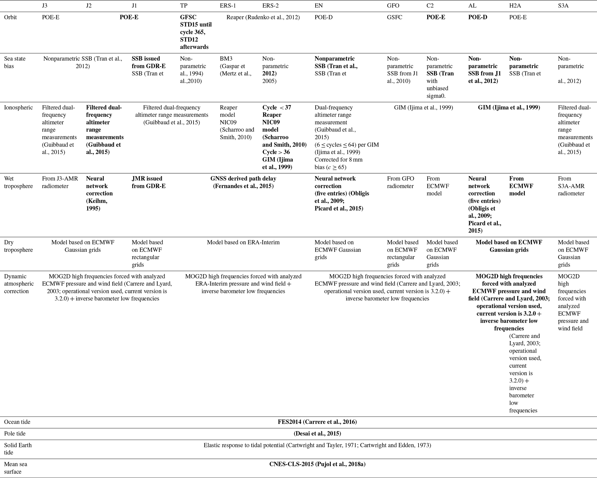
Various corrections were updated, of which the new MSS CNES-CLS-15 and ocean tide model (FES2014) have led to the greatest improvements in product quality. Valuable enhancements were made in the MSS to improve performance at short wavelengths (Pujol et al., 2018a). Furthermore, the sea level in coastal areas and the Arctic region is determined more accurately in the updated version, and errors were greatly reduced globally. Concerning the ocean tide correction, FES2014 is the latest version of the FES (finite-element solution) tide model developed between 2014 and 2016. This new release gives improved results in the deep ocean, at high latitudes and in shallow–coastal regions (Carrère et al., 2016).
2.3 Developments in DUACS processing
DUACS processing involves an initial preprocessing step during which data from the various altimeters are acquired and homogenized. Next, along-track products (L3) and multi-mission gridded products (L4) can be estimated. Finally, the derived products are computed and disseminated to users. This section is not intended to describe the entire data processing system in detail, but rather to expose the major changes made for this DT2018 version. For a detailed description of DUACS processing, readers are advised to consult Pujol et al. (2016).
2.3.1 Acquisition and preprocessing
The DUACS processing sequence can be divided into multiple steps: acquisition, homogenization, input data quality control, multi-mission cross calibration, along-track SLA generation, multi-mission mapping and final quality control.
The acquisition stage consists of retrieving altimeter and ancillary data and applying to those data the most recent corrections, models and references recommended by experts (as described in Sect. 2.1 and 2.2). This up-to-date selection is available in Table 1.
Input data quality control is a process related to the calibration–validation activities carried out for CNES, ESA and EUMETSAT. It is composed of several editing processes designed to detect and fix spurious measurements and to ensure the long-term stability of L2P products. The up-to-date editing process is described in annual Cal–Val reports for each mission (AVISO, 2017c). Since 2014, and learning from expert experience, great efforts have been made to refine this global process and notably to tailor some parts to specific regions such as high-latitude and coastal areas. At high latitudes the idea is to filter an altimeter parameter that has a specific signature for ice, compared to the ocean, and then to flag associated data as ice. But such a filtering solution affects all data, with the risk that potentially compromised data outside icy areas can be inaccurately flagged as ice. The updated development consists of using a mask so that the chosen filtering solution always provides relevant results (Ollivier et al., 2014). The mask is based on the sea ice concentration product from the EUMETSAT Ocean and Sea Ice Satellite Application Facility (OSI SAF; http://www.osi-saf.org/, last access: 9 September 2019) and gives a maximum estimation of ice extent. In coastal areas, along-track SLA measurements for non-repetitive missions were rejected for L2P DT2014 products, mainly due to the lower quality of MSS for area less than 20 km from the coast (Pujol et al., 2016). DT2018 benefits from a solution for improved MSS quality (Pujol et al., 2018a, b), so efforts were made to retain as many valid measurements as possible close to the coast. The data selection strategy is based on a median filter applied in a 30 km wide strip off the coastline (Ollivier et al., 2014). As a result, substantially more valid data can be used in DUACS, especially for geodetic measurements.
Finally, the cross-calibration step ensures that all data from all satellites provide consistent and accurate information (Pujol et al., 2016). Mean sea level continuity between altimeter missions is ensured by reducing global and regional biases for each transition between reference missions (TP–J1, J1–J2 and J2–J3). In order to minimize geographically correlated errors, two algorithms using empirical process methods are then applied, namely orbit error reduction (OER) and long-wavelength error reduction (LWER).
2.3.2 Along-track product generation
The along-track generation for repetitive altimeter missions is based on the use of a mean profile (MP) (Table 2; Pujol et al., 2016; Dibarboure and Pujol, 2019). These MPs are necessary in order to colocate the sea surface heights of the repetitive tracks and to retrieve a precise mean reference in order to compute sea level anomalies. The methodology used to compute the DT2018 MP was the same as for DT2014. The differences arise from the upstream measurements, as new altimetry standards were used in DT2018 (described in Sec.t 2.2), along with new data selection (Sect. 2.3.1) and reviewed temporal periods for the different altimeters considered. Table 2 presents the altimeter missions and time periods used to compute the four different MPs available along the following tracks: TOPEX–Poseidon, Jason1, OSTM–Jason2, Jason3, TOPEX–Poseidon interleaved phase, Jason1 interleaved, Jason2 interleaved, ERS-1, ERS-2, Envisat, SARAL–ALtiKa and Geosat follow-on.
Table 2Time periods and cycles used to compute the mean profile in the DT2018 version.
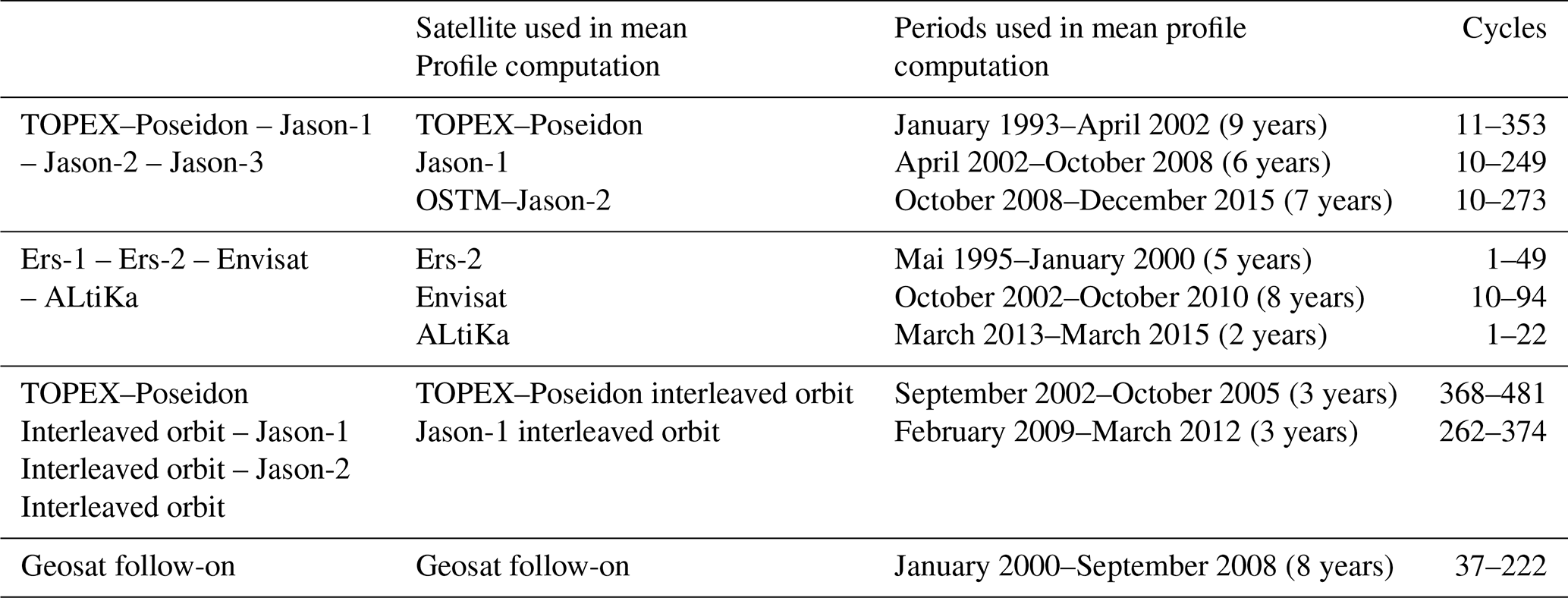
Following the previous MPs version, additional measurements collected by OSTM–Jason-2 and SARAL–ALtiKa between 2012 and 2015 were exploited for DT2018. Since March 2015, however, ALtiKa has been considered a non-repetitive mission for delayed-time products. As a result, no measurements after that date were taken into account when computing the ERS-1–ERS-2–EN–AL MP. To limit the ionospheric correction error in this MP, no ERS-2 data collected between January 2000 and October 2002 were used to compute the MP because the ionospheric activity was much more intense during this period than between 1995 and 2000.
New DT2018 MPs were defined as close to the coast as possible as illustrated in Fig. 2. This improvement is associated with the use of the new MSS (Pujol et al., 2018a) and ocean tide correction as well as the refined selection of valid data (Sects. 2.2 and 2.3.1). It has a direct and positive impact on along-track product generation that provides extended coastal coverage. Globally, comparisons at crossovers provide good results in this new version. Compared to the DT2014 version, we observe a decrease in the mean of the difference at crossovers by around 0.3 cm globally and up to 1 cm locally (data not shown here).

Figure 2Gain of measurements in the TOPEX–Poseidon–Jason1–OSTM–Jason-2 mean profile used in DT2018 compared to DT2014. Gain of points in DT2018 is in red, loss of points is in blue.
It should be noted that for the Sentinel-3A, it was impossible to estimate a precise MP for this reprocessing due to the short time period (i.e., a few months) available to compute it. Consequently, data from the Sentinel-3A mission were only interpolated into theoretical positions (Dibarboure et al., 2011), and then the gridded MSS (Pujol et al., 2018b) was removed. Since the reprocessing, an MP has been calculated (Dibarboure and Pujol, 2019; Pujol et al., 2018b) and the Sentinel-3A dataset has been reprocessed in a CMEMS version in 2019.
For non-repetitive missions (ERS-1 during its geodetic phase, Cryosat-2, Hayaing-2A, both Jason-1 and Jason-2 in their geodetic phase, and SARAL–ALtiKa in its geodetic phase), no MP can be estimated. The SLA is in this case derived along the real altimeter tracks using the gridded MSS (Pujol et al., 2016; Dibarboure and Pujol, 2019).
The final step of along-track processing consists of noise reduction using low-pass Lanczos filtering and subsampling. This process remains unchanged from the DT2014 version (Pujol et al., 2016).
DT2018 reprocessing was also an opportunity to propose new products. New along-track products were tailored for assimilation purposes to provide users with the specific geophysical corrections used to compute the sea level anomaly in the DUACS processing: DAC, ocean tide and LWER. As explained in Sect. 2.2, these geophysical effects are taken into account in DUACS because their temporal variability is too high to be resolved by altimeter measurements and to be mapped using the OI method.
2.3.3 Gridded product generation: multi-mission mapping
The multi-mission mapping procedure in DUACS is based on an optimal interpolation (OI) technique derived from Le Traon and Ogor (1998), Ducet et al. (2000), and Le Traon et al. (2003). This method is designed to generate regularly gridded products for sea level anomalies by combining measurements from different altimeters. The main objective in the DT2018 reprocessing framework was to improve gridded altimetry products in the tropics, in coastal areas and at the mesoscale. To do so, OI parameters were adjusted. The sea level spatial and temporal variability were more accurately defined based on the 25 years of observations available. Particular attention was paid to coastal areas, where spurious peaks of high variability were able to be reduced. An optimized selection of along-track data was incorporated into OI processing by changing the size of the suboptimal interpolation window, decreasing it by one-third in regions of high variability and in the equatorial belt.
OI observation errors were increased in the equatorial belt, as the impact of filtering and subsampling had been previously underestimated in this area where they generate noise at small scales in gridded products. Errors generated when using the gridded MSS were updated with the use of the new MSS version (Pujol et al., 2018a).
Correlation scales were only reviewed for regional Mediterranean products. While set to constant values (100 km and 10 ds) in the DT2014 version, precise covariance and propagation models were computed for DT2018 regional mapping. Spatial scales now range from 75 to 200 km, while temporal scales remain at 10 d. These changes have contributed to improving the retrieval of mesoscale signals in Mediterranean regional products (Sect. 4).
For Black Sea processing, OI parameters are now similar to parameters used for the global ocean processing, except for the correlation scales, which are still set to 100 km and 10 d.
2.4 Different products for different applications
Two different types of sea level gridded altimetry products are available in DT2018 version. The first type, produced and distributed within the Copernicus Marine Service (CMEMS), is dedicated to mesoscale observation. The other type, produced and distributed within the Copernicus Climate Change Service (C3S), is dedicated to monitoring the long-term evolution of the sea level for use in climate applications and for analyzing ocean–climate indicators (such as global and regional MSL evolution). Two types of altimeter processing configurations are exploited to build these two products. The first difference of configuration is related to the number of altimeters used in the satellite constellation.
Mesoscale observation requires the most accurate sea level estimation at each time step, along with the best spatial sampling of the ocean. All available altimeters are thus included in CMEMS products, and the sampling can vary with time depending on the constellation status. In contrast, the temporal stability of surface sampling is more important when monitoring the long-term sea level evolution. A steady number of altimeters (two) is thus used in C3S products. This corresponds to the minimum number of satellites required to retrieve mesoscale signals in delayed-time conditions (Pascual et al., 2006; Dibarboure et al., 2011). Within the production process, long-term stability and large-scale changes are established on the basis of records from the reference missions (TOPEX–Poseidon, Jason-1, Jason-2 and Jason-3) used in both CMEMS and C3S products. Any additional missions (e.g., as many as five additional missions in 2017) are then homogenized with respect to the reference missions and help to improve mesoscale process sampling, providing high-latitude coverage and increasing product accuracy. However, the total number of satellites has greatly varied over the altimetry era and biases may develop when a new satellite on a drifting orbit is introduced. Each addition may affect the stability of the global and regional MSL by several millimeters (data not shown here). Although spatial sampling is reduced when there are fewer satellites, the risk of introducing such anomalies is thus also reduced in C3S products, resulting in improved stability. In CMEMS products, stability is ensured by the calibration with the reference missions, and mesoscale errors are reduced due to the improved ocean surface sampling made possible by using all the satellites available in the constellation.
As a second difference of configuration, the reference used to compute sea level anomalies for C3S products was an MSS for all missions, whereas for CMEMS products, an MP was used along the theoretical track of satellites following a repetitive orbit (see Sect. 2.3.2). Considering the regional mean sea level temporal evolution, the combined use of MSS and MP for successive missions in the merged product gives rise to regional centimetric bias (data not shown here). Consequently, the systematic use of MSS for all missions has been privileged in the C3S products to ensure MSL stability, and the use of MP for repetitive missions has been selected in the CMEMS products to increase their accuracy.
The differences between CMEMS and C3S product quality are discussed on a climate scale in Sect. 3.4.
This section focuses on the quality of gridded (L4) products. Sea surface height and derived current products were analyzed at different spatial scales (open ocean, coastal areas), distinguishing different temporal scales (from mesoscale to climatic scales). DT2018 L4 products were compared with those of DT2014 over the 1993–2017 time period. Except when explicitly mentioned otherwise, the results presented in this section are valid for all DUACS DT2018 products distributed via both Copernicus services.
3.1 Mesoscale signals in along-track and gridded products
Optimizing the mapping process (Sect. 2.3.3) and incorporating the new altimetry corrections (Sect. 2.2) had a direct impact on the observation of ocean sea level and surface circulation dynamics in the gridded products. To characterize this impact, the difference between DT2014 and DT2018 temporal variability is shown in Fig. 3. An additional variance between 2 % and 5 % is observed for high-variability regions in DT2018 products. This increase is due to having changed the OI spatial and temporal scales used in the mapping process and decreased the suboptimal interpolation window size. The OI selection window is more focused on close observations (both spatial and temporal). In coastal areas, a substantial reduction in SLA variance is observed due to both the FES2014 tidal correction and, to a more limited extent, the new MSS. For the tidal correction, Carrere et al. (2016) have shown a reduction in SLA variance at nearshore crossovers. Pujol et al. (2018a) have emphasized that the new gridded MSS shows less SLA degradation near the coast. These improved standards contribute to a valuable local reduction in SLA variance (up to 50 % alongshore). At high latitudes, the difference of variance is significant (±100 to ±200 cm2) and is due to the new MSS correction. Indeed, Pujol et al. (2018a) have shown that the CNES_CLS 2015 MSS improves both coverage in the Arctic and the resolution of the shortest wavelengths at high latitudes.
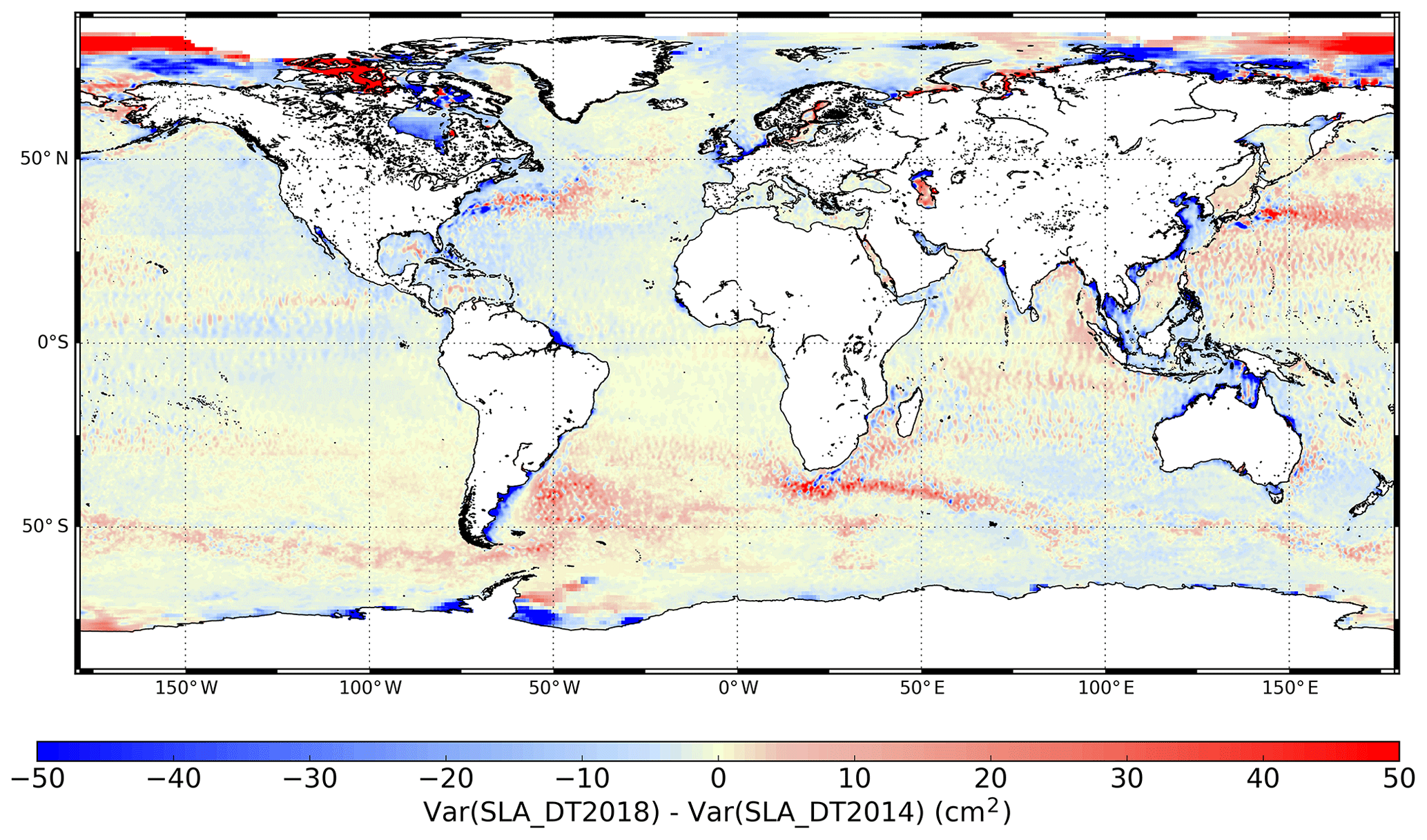
Figure 3Difference between SLA variance observed with DT2018 gridded products and SLA variance observed with DT2014 gridded products over the 1993–2017 period.
Compared to DT2014, the new version reveals more intense western boundary currents (geostrophic part). This has a direct impact on the eddy kinetic energy (EKE) derived from these products. Figure 4 presents the spatial difference in the mean EKE over the global ocean between DT2018 and DT2014 products, along with their temporal evolution. As observed before for the differences of SLA variance, a higher energy is evident in high-variability areas. This corresponds to a 2 % increase in EKE in DT2018. However, in the equatorial belt (±20∘ N), the EKE in DT2018 is lower (−17 %). This is a direct consequence of the noise measurement that is taken into consideration in the mapping process for all satellites: observation errors prescribed during OI in the tropical belt have been increased, so the SLA signal is smoother and less energy is observed in this region. In coastal areas, the DT2018 version presents fewer spurious peaks of high EKE (Fig. 4b). As already stated, this is related to the improved altimetry correction and lower SLA variance. Considering the mean EKE time series, a global reduction of 26 cm2 (17 %) is observed for dataset DT2018. This is directly due to the lower tropical EKE. Another important point to note is that the standard deviation of EKE in these products is lower than in DT2014. This illustrates that EKE variations are less important, and there are fewer isolated anomalies (and these are mostly coastal) in the new DT2018 products.
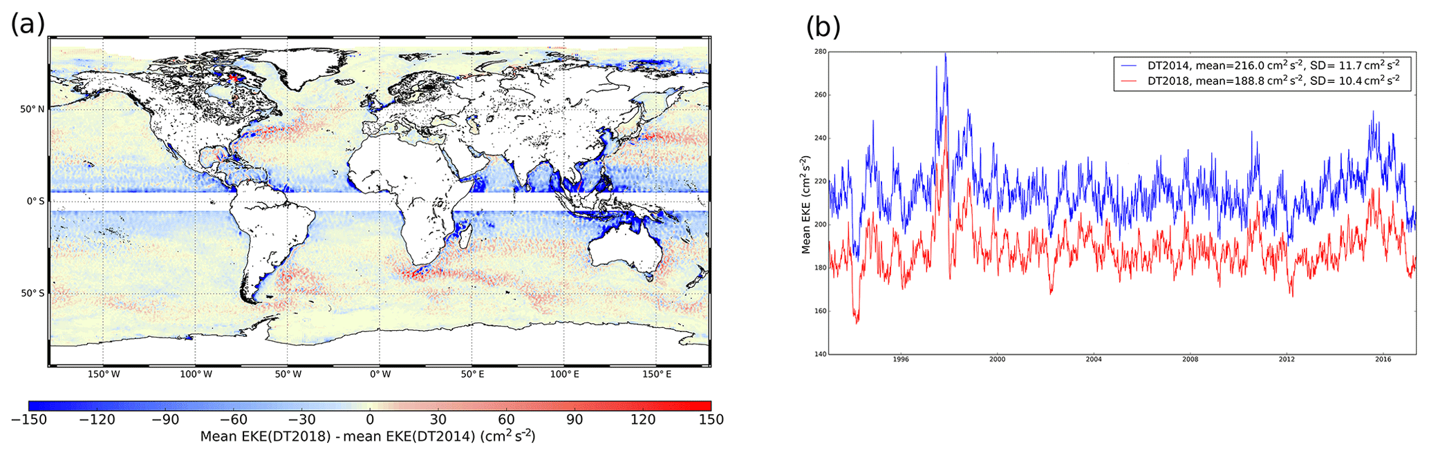
Figure 4Map of the difference between mean EKE for DT2018 and DT2014 gridded products (a) and the evolution of the mean EKE over the global ocean, computed from DT2014 (blue line) and DT2018 (red line) SLA gridded products (b) over the 1993–2017 period. The ±5∘ N equatorial belt has been removed.
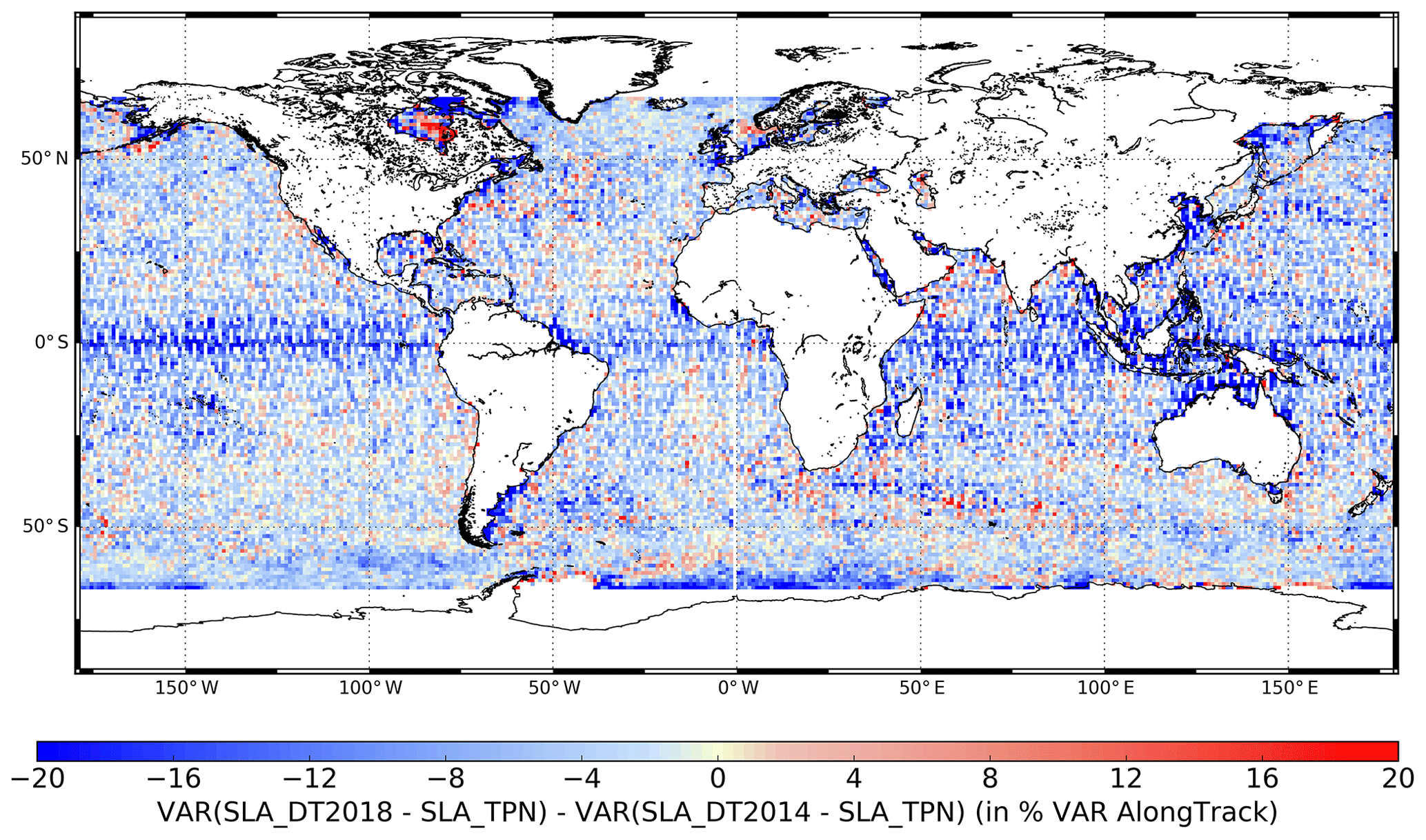
Figure 5Difference of the RMS of the difference between gridded SLA products and independent TOPEX–Poseidon interleaved along-track SLA measurements successively using the DT2018 and DT2014 versions. Negative values represent reduced differences between DT2018 altimetry products and independent along-track measurements.
The gridded SLA accuracy was estimated by comparison with independent along-track measurements. Maps produced by merging only two altimeters were compared with SLAs measured along-track from the tracks of another mission that was kept independent from the mapping process (see Pujol et al., 2016, for the full methodology). TOPEX–Poseidon interleaved was compared with gridded products that merged Jason-1 and Envisat over 2003–2004. It must be pointed out that these results are much more representative of gridded products combining two altimetry missions. Products combining all available missions can usually benefit from improved sampling when three to six altimeters are used. The errors described here should thus be considered the upper limit. Table 3 summarizes the results of comparisons over different areas. Figure 5 shows the percentage of the difference in variance between gridded products and TP independent along-track measurements for DT2018 and DT2014 products. The gridded product error for mesoscale wavelengths ranges between 1.4 cm2 (for a low-variability area) and 37.7 cm2 (for a high-variability region). The improvements in DT2018 compared with DT2014 affect all areas. Offshore, the improvement is fairly low (around 3 %) and is associated with the enhanced version of the OI mapping parameter. In coastal areas, the improvements are more significant (around 10 %) and caused by the new tidal correction (FES2014) and, to a lesser extent, the MSS and MPs. In the tropical belt, improvements are also significant (around 9 %) and related to the observation errors that were increased in this area for the OI processing.
Table 3Variance of the differences between gridded (L4) DT2018 two-satellite merged products and independent TP interleaved along-track measurements for different geographic selections (cm2). In parentheses: variance reduction (%) compared with the results obtained with the DT2014 products. Statistics are presented for wavelengths ranging 65–500 km and after latitude selection (|LAT∘).
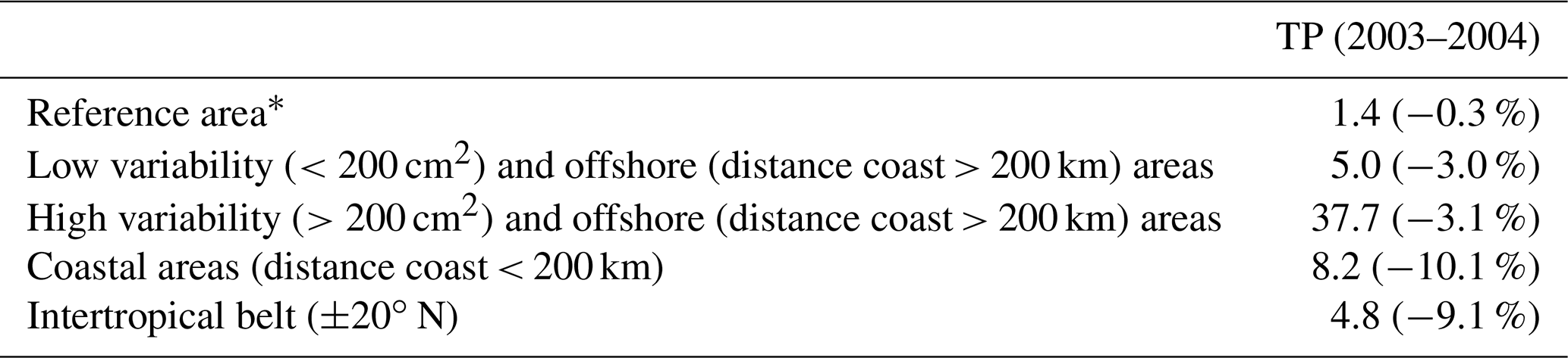
* The reference area is defined by 330–360∘ E, −22 to −8∘ N and corresponds to a very low-variability area (between 0 and 7 cm2) in the South Atlantic subtropical gyre where the observed errors are small.
3.2 Geostrophic current quality
Absolute geostrophic currents for DT2018 were assessed using drifter data for the 1993–2017 time period. The AOML (Atlantic Oceanographic & Meteorological Laboratory) database was used for the comparison (Lumpkin et al., 2013). These in situ data were corrected for Ekman drift (Rio et al., 2011) and wind if a drifter's drogue had been lost (Rio, 2012) so as to be comparable with the altimetry absolute geostrophic currents. Drifter positions and velocities were interpolated using a 3 d low-pass filter in order to remove high-frequency motions (Rio et al., 2011). The absolute geostrophic currents derived from altimetry products were then interpolated onto drifter positions for comparison.
The distribution of the current's intensity shows an overall underestimation of magnitude in altimetry products compared to drifter observations (data not shown). Figure 6 shows the RMS difference between the DT2018 geostrophic current and that of drifters. The mean RMS is nearly 10 cm s−1 and the main errors are located nearshore and in a high-variability region with peaks higher than 20 cm s−1. Taylor skill scores (Taylor, 2001) were computed for the zonal and meridional components of the current in DT2018. This assessment took into consideration both the signal's correlation and its standard deviation. Results are quite robust: 0.89 for the zonal and 0.87 for the meridional component.
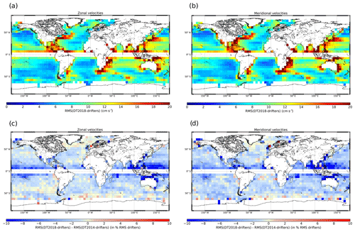
Figure 6Zonal (a) and meridional (b) RMS of the difference between DUACS DT2018 absolute geostrophic current and drifter measurements over the 1993–2017 period. Zonal (c) and meridional (d) difference of the RMS of the altimeter geostrophic currents minus drifters measurements successively using the DT2018 and DT2014 gridded products. Negative values represent reduced differences between DT2018 altimetry products and drifters. The statistic is expressed as a percentage of the RMS of drifter measurements. Statistics have been computed in boxes of 5∘ × 5∘. Boxes with fewer than 1000 points have been masked.
Table 4 summarizes the mean RMS of the differences between geostrophic current maps and drifter measurements over different areas for versions DT2018 and DT2014. DT2018 products are more consistent with drifter measurements than DT2014 version products. The improvement is clearly visible in the intra-tropical belt. The variance of the differences with drifters is reduced around 20 % to 40 % in this area. Additional noise-like signals present in the DT2014 version had reduced consistency with drifter measurement (Pujol et al., 2016). This degradation was corrected for by the change in mapping parameters used for this updated version (Sect. 2.3.3). A significant improvement can also be observed in coastal areas, where the variance of differences with drifter measurements is reduced by nearly 15 % (Table 4). Elsewhere, this reduction in the variance of difference ranges from 4 % to 7 %.
Table 4Variance of the differences between gridded geostrophic current (L4) DT2018 products and independent drifter measurements (cm2 s−2). In parentheses: variance reduction (%) compared with the results obtained with the DT2014 products. Statistics are presented for latitude selection (5∘ N < |LAT| < 60∘ N).
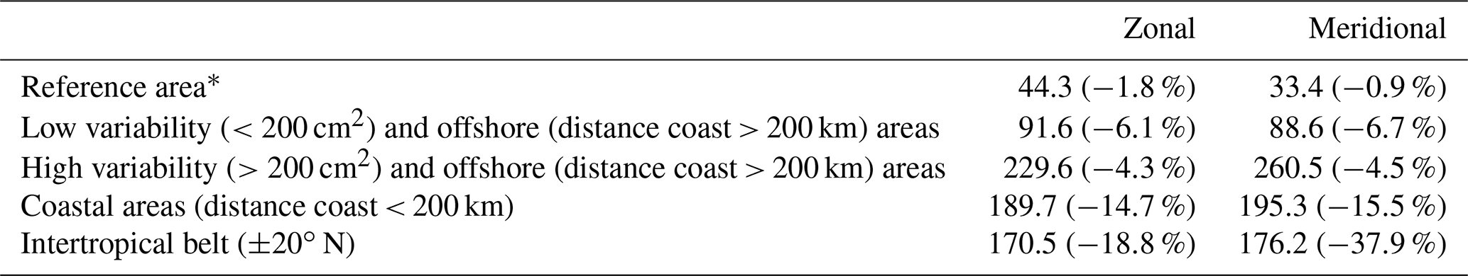
* The reference area is defined by 330–360∘ E, −22 to −8∘ N and corresponds to a very low-variability area (between 0 and 7 cm2) in the South Atlantic subtropical gyre where the observed errors are small.
3.3 Coastal areas
As described in Sect. 2.3.1 and 2.3.2 the new DUACS DT2018 processing has a key impact on coastal areas, and overall, all missions have more measurements available in DT2018 compared to DT2014.
The assessment of gridded products in coastal areas included a comparison with tide gauge (TG) measurements. We used mean monthly TG measurements from the PSMSL network (Permanent Service for Mean Sea Level; PSMSL, 2016) from 1993 to 2017. We used only long-term monitoring stations with a lifetime of more than 2 years. Sea surface height measured by TG was compared with gridded SLA by considering the maximum correlation with the nearest neighboring pixel (Valladeau et al., 2012; AVISO, 2017a). In Fig. 7 the variance of the difference between DT2018 altimetry products and TG measurements is compared with that obtained from the differences using DT2014 altimetry products. The results show a global reduction in the variance (0.6 %) when DT2018 data are used. There is a clear improvement along the Indian coast, Oceania and northern Europe. Local degradation can be observed along the coast of Spain and along the US west coast. These degradations, which are not observed in other diagnoses such as independent along-track measurements, still need to be further investigated.
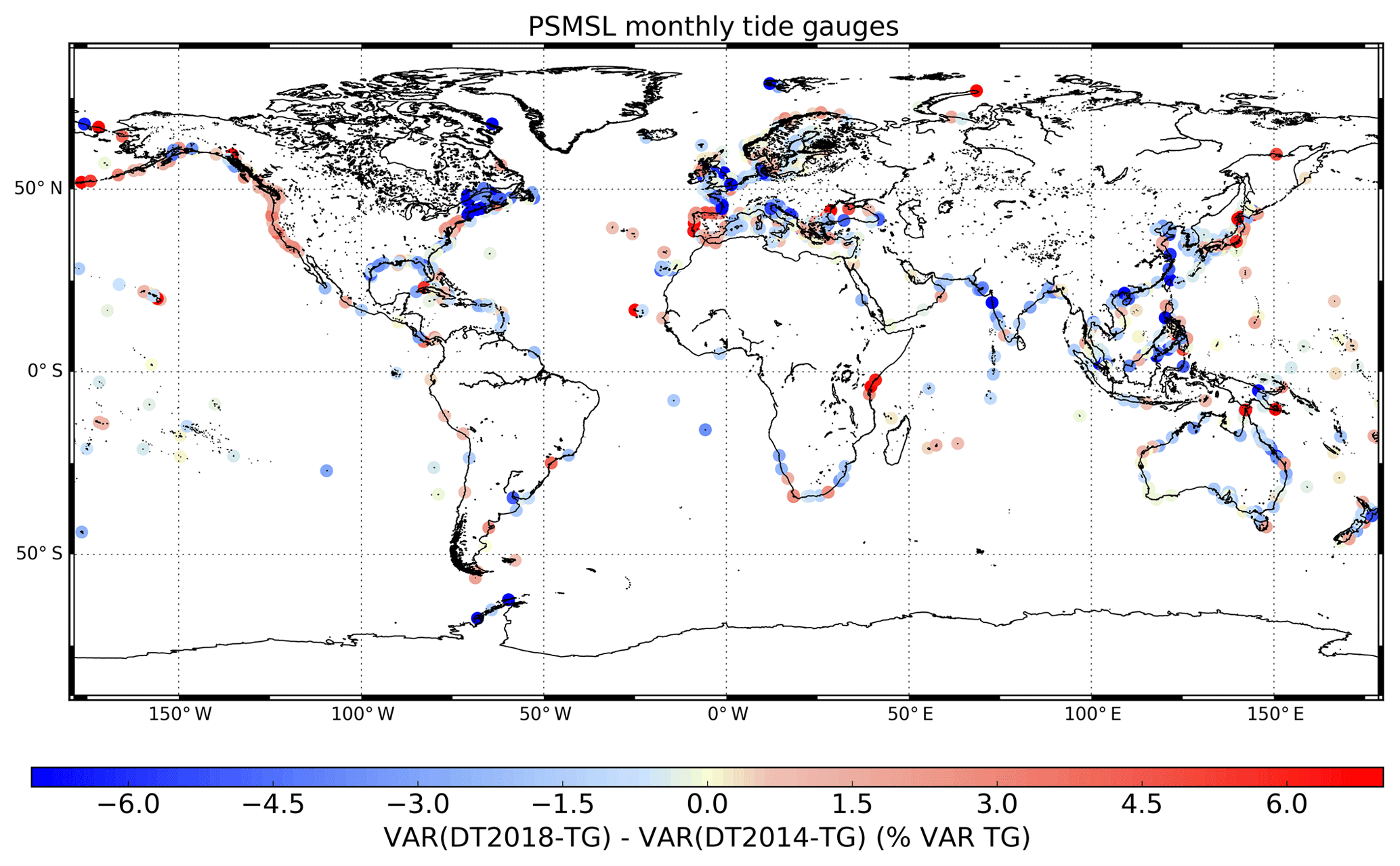
Figure 7Difference of the variance between gridded SLA products and TG successively using the DT2018 and DT2014 gridded products. We used mean monthly TG measurements from the PSMSL network. Negative values represent reduced differences between DT2018 altimetry gridded SLA and TG. The statistic is expressed as a percentage of the RMS of TG measurements.
3.4 Climate scales
The global mean sea level (GMSL) is a key indicator of climate change since it reflects both the amount of heat added in the ocean and the land ice melt coming mainly from Antarctic and Greenland ice sheets and glaciers. Three different altimeter products can be used to compute three GMSL estimates: the time series of the box-averaged along-track measurements of the reference missions only (Ablain et al., 2017) and L4 merged gridded sea level products from CMEMS and C3S (e.g., Fig. 8a). For the same product versions and computation periods, these three GMSL estimates are considered to be equivalent since almost the same altimetry standards are used to compute sea level anomalies, and the long-term stability for all products is ensured by using the same reference missions. The remaining GMSL differences observed (∼0.17 mm yr−1) are not significant given the uncertainty on different scales (the uncertainty in the GMSL trend is 0.4 mm yr−1 at the 90 % confidence level given by Ablain et al., 2019). Note that as previously mentioned (Sect. 2.4), differences can be found between the two different Copernicus gridded products (CMEMS–C3S) when computing regionally averaged MSL.
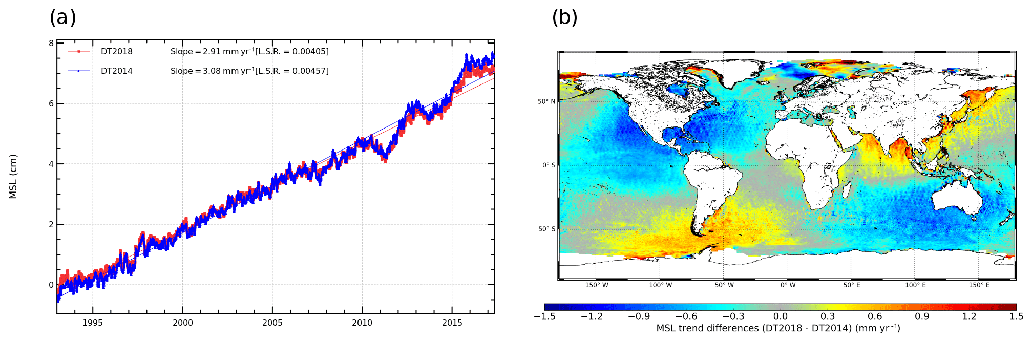
Figure 8(a) Temporal evolution of the GMSL estimated from DT2018 (red line) and DT2014 (blue line) gridded SLA products. The annual and semi-annual signals were adjusted and no GIA correction was applied. (b) Map of the differences of the local MSL trend estimated from the DT2018 and DT2014 gridded SLA products. MSL was estimated over the 1993–2017 period.
When computing area-averaged MSL time series, users are advised that DUACS products are not corrected for the effect of glacial isostatic adjustment (GIA) due to post-glacial rebound. A GIA model should be used to estimate the associated sea level trends.
In addition, between 1993 and 1998, GMSL is known to have been affected by instrumental drift in the TOPEX-A measurement, as quantified by several studies (Watson et al., 2015; Beckley et al., 2017; Dieng et al., 2017). The sea level altimetry community agrees that it is necessary to correct the TOPEX-A record for instrumental drift to improve accuracy and reduce uncertainty in the total sea level record. However, there is no consensus so far on the best approach to estimate drift correction at global and regional scales. DUACS sea level altimetry products are not corrected for TOPEX-A drift, pending ongoing TOPEX reprocessing by CNES and NASA/JPL, but users can apply their own correction. Adjusting for this TOPEX-A anomaly creates a GMSL acceleration of 0.10 mm yr−2 for the 1993–2017 time span that does not otherwise appear (WCRP Global Sea Level Budget Group, 2018).
Figure 8a shows the GMSL temporal evolution and associated trend computed with the new DT2018 and former DT2014 versions of DUACS C3S products. In the latest version, the global mean sea level trend is 3.3 mm yr−1 (including GIA correction of −0.3 mm yr−1). The origin of the associated uncertainty is discussed by Legeais et al. (2018b). The map of the differences for the local MSL trend derived from the latest and previous product versions (Fig. 8b) displays a pattern predominantly associated with the different orbit standards used in the two product versions (GDR-E versus GDR-D; see Table 1). Such a result is confirmed by comparing altimetry products with the independent dynamic height measurements derived from in situ Argo profiles (Valladeau et al., 2012; Legeais et al., 2016).
4.1 SLA field quality
As previously discussed for global ocean products, the quality of regional gridded SLA products is estimated through comparison with independent altimeter along-track and tide gauge measurements.
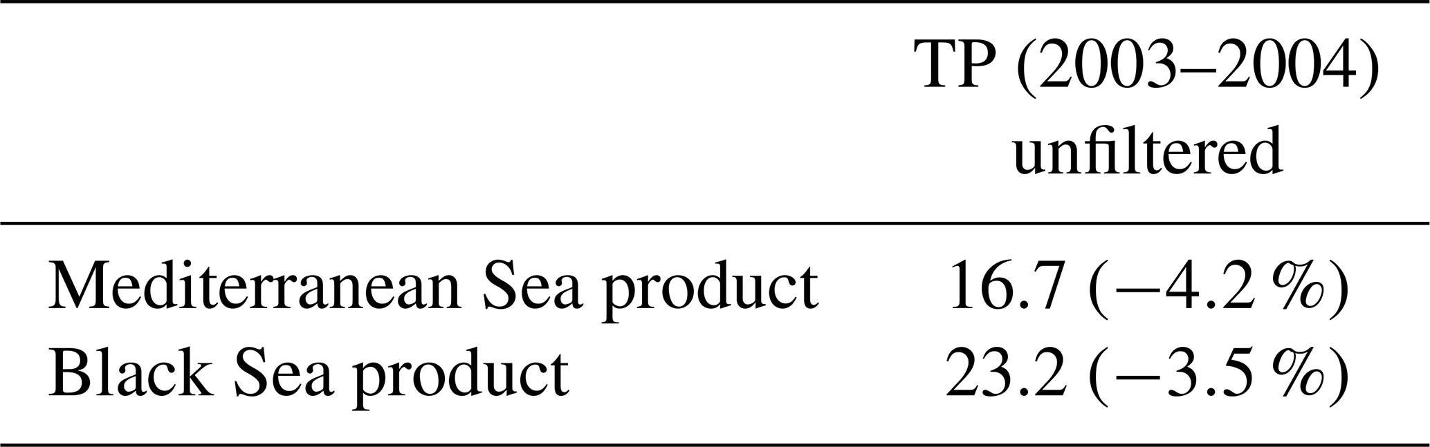
Figure 9 shows the spatial distribution of the RMS of the differences between regional DT2018 SLA gridded products and independent along-track measurements (TOPEX–Poseidon interleaved along-track measurements over the 2003–2004 period). The main statistics for these comparisons, as well as a comparison with the previous DT2014 version, are also given in Table 5. In contrast with the global products assessment, the evaluation of regional products cannot include the mesoscale signal analysis: the short length of the tracks segments available over the regional seas does not allow for the accurate filtering of the signal in order to focus specifically on the mesoscale. The results obtained show that for the DT2018 Mediterranean product, the main errors are located in coastal areas and in the Adriatic and Aegean seas, with RMS values ranging from 6 to 9 cm. The Black Sea products also show higher errors in coastal areas (results not shown here). The mean variance of the differences between gridded products and along-track measurements is nearly 17 and 23 cm2 over the Mediterranean Sea and the Black Sea. This value is higher than the mean error observed over low-variability areas in the global ocean (Table 3), mainly due to the different wavelengths addressed in these comparisons. Compared to the previous regional DT2014 version, the error is reduced by 4.2 % for the Mediterranean Sea and 3.5 % for the Black Sea. It is important to note that these results are representative of gridded product quality when only two altimeters are available. These products can be considered to be degraded products for mesoscale mapping since they use minimal altimeter sampling.
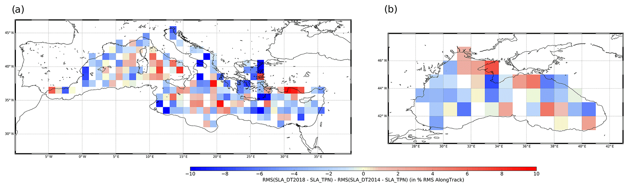
Figure 9Difference of the RMS of the difference between gridded regional Mediterranean Sea (a) and regional Black Sea (b) SLA products and independent TOPEX–Poseidon interleaved along-track SLA measurements successively using the DT2018 and DT2014 versions. Negative values represent reduced differences between DT2018 altimetry products and independent along-track measurements. The statistic is expressed as a percentage of the RMS of the independent along-track product.
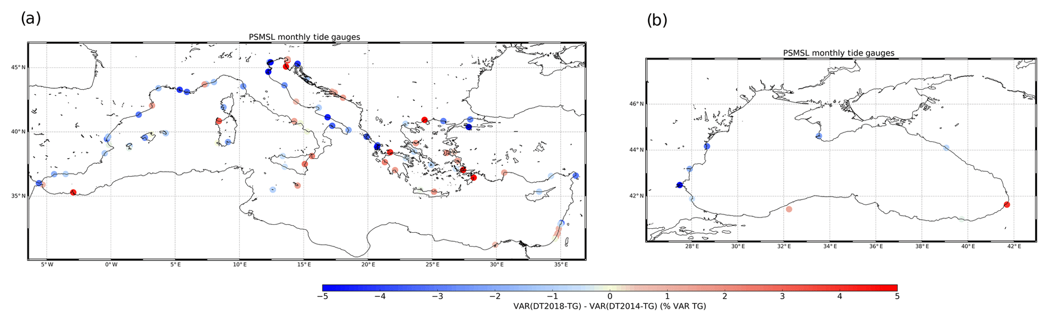
Figure 10Difference of the variance between regional Mediterranean gridded (a) and regional Black Sea (b) SLA products and TG successively using DT2018 and DT2014 gridded products. We used mean monthly TG measurements from the PSMSL network. Negative values represent reduced differences between DT2018 altimetry gridded SLA and TG. The statistic is expressed as a percentage of the RMS of TG measurements. The statistic is expressed as a percentage of the RMS of the independent along-track product.
Table 5Variance of the differences between gridded (L4) DT2018 two-satellite merged regional Mediterranean and Black Sea products and independent TP interleaved along-track measurements without filtering over the time period 2003–2004 (cm2). In parentheses: variance reduction (%) compared to the results obtained with the DT2014 products.
Compared to the previous version, consistency with monthly TG measurements (Fig. 10) is improved locally in the regional DT2018 Mediterranean gridded product in the western part of the Mediterranean basin. Degradation is observed, however, in some other coastal areas, especially in the center of the basin and along the Turkish coast. For the Black Sea gridded product, only nine tide gauges were available for the comparison. With the exception of a tide gauge at the eastern end of the Black Sea on the Georgian coast, these DT2018 regional products are improved of the order of 1 %.
4.2 Geostrophic current quality in the Mediterranean Sea
DT2018 regional absolute geostrophic current in the Mediterranean basin was assessed using drifter data for the 1993–2017 period. The data were collected from drifters released in the Mediterranean Sea as part of the AlborEx (Pascual et al., 2017) and MEDESS-GIB (EU MED Program; http://www.medess4ms.eu/, last access: 9 September 2019; Sotillo et al., 2016) multi-platform experiments as well as other experiments incorporated into CMEMS In Situ Thematic Centre (INS TAC) products. These data are processed similarly to the global product (Sect. 3.2).
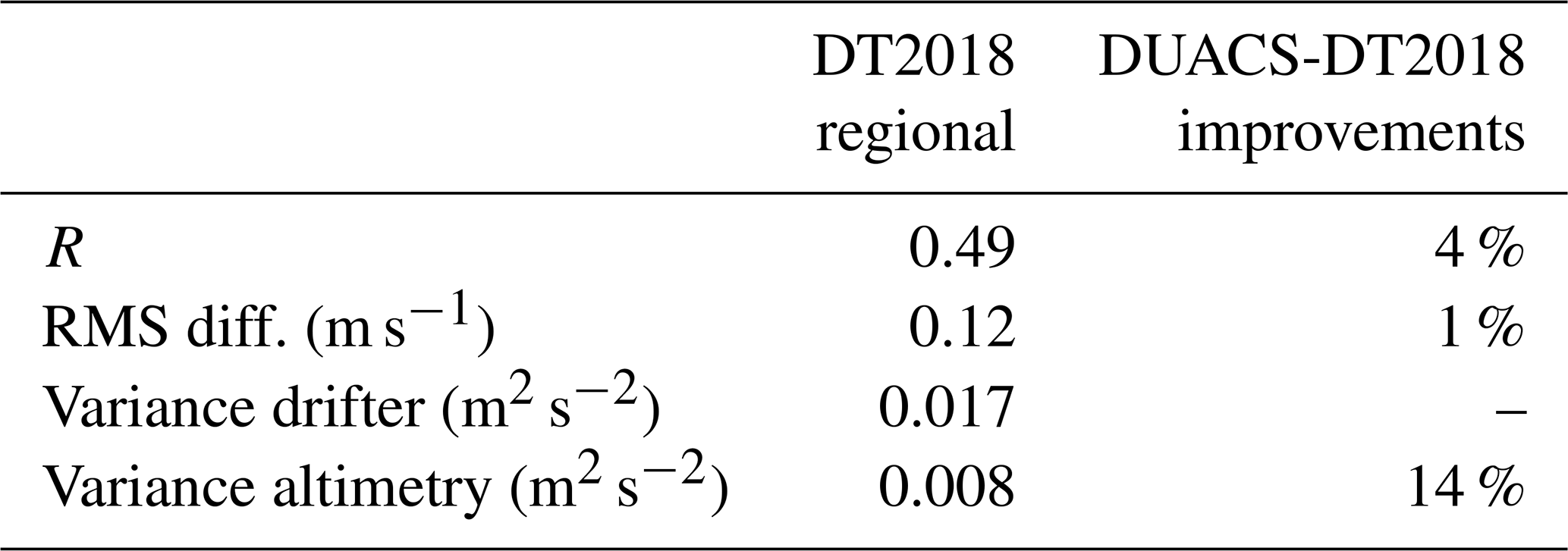
Table 6 summarizes the main statistical results for the whole basin. The DT2018 regional product presents a correlation coefficient with drifter data 4 % greater than that obtained when using the DT2014 regional product. Moreover, the errors in the later version are slightly lower at 1 %, whilst its improvement in explained variance is as high as 14 %.
Table 6RMSE (m s−1) and correlation coefficient between the absolute geostrophic velocities derived from DT2018 regional products for the Mediterranean Sea, as well as absolute surface velocities as obtained from drifters collected in the basin. The variance of the datasets (m2 s−2) and the data used to conduct the comparison is also displayed.
The analysis was then repeated for the different dynamical subregions of the basin (see Fig. 11a) reported by Manca et al. (2004). This differentiation is based on the typical permanent features in the upper 200 m of the water column. Overall, comparisons between geostrophic velocities derived from the DT2018 regional product and absolute surface velocities retrieved by the drifters (Fig. 11b–e) reveal a correlation coefficient greater than 0.40 in most of the boxes. Correlations greater than 0.50 are mainly located in the southernmost part of the basin where stronger mesoscale activity occurs, namely the Alboran Sea (DS1), the Algerian Basin (DS3 and DS4), the Sardinian Channel (DI1), the Strait of Sicily (DI3), the Ionian Sea (boxes DJ7, DJ8 and DJ5) and the Cretan passage (DH3). The overall RMS difference between the two datasets ranges between 8 and 11 cm s−1, although it reaches 20 cm s−1 in DS1 due this area's strong dynamics. Slightly larger errors are obtained when comparing the DT2014 product with drifter observations (not shown here). Furthermore, drifter data collected in boxes DS1, DS3 and DS4 have the largest variability due to the aforementioned mesoscale activity. This fact is also reflected in the two altimetry products, which have the largest variance values in the Mediterranean basin.
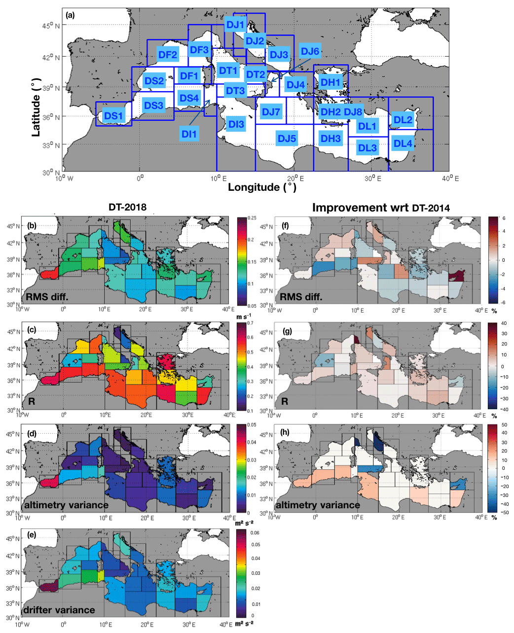
Figure 11(a) Map of the Mediterranean Sea showing the geographical limits and the nomenclatures of the regions (blue boxes) as defined in Manca et al. (2004) wherein drifter data are available in the western sub-basin: Alboran Sea (DS1), Balearic Sea (DS2), western and eastern Algerian (DS3 and DS4), Algero–Provençal (DF1), Liguro–Provençal (DF3, DF4), Gulf of Lion (DF2), Tyrrhenian Sea (DT4), Sardinian channel (DI1), Tyrrhenian Sea (DT2, DT3), and the Strait of Sicily (DI3). In the eastern sub-basin: Adriatic Sea (DJ1–DJ3), Ionian Sea (DJ4–DJ8), Aegean Sea (DH1, DH2), Cretan Passage (DH3) and Levantine basin (DL1–DL4). (b–e) Maps of the Mediterranean Sea showing the comparison between the DT2018 regional altimetry product and the drifter in situ observations within the geographical limits and the nomenclatures of the regions defined in (a). The statistical parameters shown are (b) RMS difference, (c) correlation coefficient, (d) altimetry variance and (e) drifter variance. (f–h) Improvements (%) of the comparisons between the DT2018 regional product and drifter in situ observations with respect to the comparisons by using the DT2014 product within the geographical limits and the nomenclatures of the regions defined in (a). The statistical parameters shown are (f) RMS difference, (g) correlation coefficient and (h) altimetry variance. Positive values denote an improvement of the DT2018 regional product over DT2014.
Overall, the correlation coefficient between the DT2018 regional product and in situ drifter data is improved by 5 %–10 % with respect to that obtained when using the DT2014 product (Fig. 11g). Here, positive values denote an improvement in DT2018 over DT2014. This fact is mainly observed in areas of strong mesoscale activity. Moreover, the errors (Fig. 11f) are reduced by 2 % in the northernmost part of the western Mediterranean basin and Adriatic Sea. However, negative values lower than 2 % (slightly larger errors when using DT2018) are observed in the Algerian Basin and most of the eastern part of the Mediterranean basin. The main improvement in DT2018 with respect to DT2014 lies in the variance explained (Fig. 11h), which presents values nearly 20 % higher in the later product in some areas of the western part of the basin and nearly 10 % higher in the eastern part. This is due to the better capturing of mesoscale activity. This improvement is not observed in the northernmost part of the basin, where less mesoscale activity occurs.
More than 25 years of level 3 and level 4 altimetry products were reprocessed and delivered as version DT2018. This reprocessing takes into account the most up-to-date altimetry corrections and also includes changes in the mapping processing parameters. These changes impact SLA signals at multiple temporal and spatial scales.
A notable change concerns the gridded sea level altimetry products that are available in version DT2018. They are produced and distributed through two different Copernicus services that correspond to different applications. CMEMS distributes maps that include all the available altimeter missions. These maps provide the most accurate sea level estimation with the best spatial and temporal sampling of the ocean at all times. Through C3S, maps that include only two satellites are used to compute the most homogeneous and stable sea level record over time and space. Sea level C3S products are dedicated to monitoring long-term sea level evolution for climate applications and analyzing ocean–climate indicators (such as global and regional MSL evolution).
Other changes were implemented in DT2018 processing: the altimetry standards and geophysical corrections were brought up to date with expert recommendations, and mapping parameters, including spatial and temporal correlation scale and measurement errors, were refined. We also focused on improving coastal editing to obtain many relevant sea level data, mainly from drifting altimeters. Additional sea level data were incorporated into DT2018, in particular Sentinel-3A measurements taken over a 6-month extension period.
Discussing these key changes, we then focused on describing their impact on gridded sea level products. SLA variability has increased in energetic areas (from 5 % to 10 %) and decreased locally along coasts (up to 50 %). A 10 % EKE decrease in the equatorial belt has also been observed and is related to the reduced measurement errors prescribed for OI in this area.
To achieve independent comparisons, geostrophic currents were examined in comparison to in situ observations. Compared to the version DT2014, offshore improvements (+4 %–5 %), particularly in the tropics (+5 %–10 %), and coastal improvements (+10 %) have been demonstrated using independent drifter data. An independent along-track sea level comparison and tide gauge comparisons have strengthened these conclusions.
Regional products are also enhanced with DT2018, taking advantage of new standards and processing. The SLA gridded product errors in the regional products have decreased by 3 % to 4 % when estimated using independent along-track measurements.
The limitations exposed by Pujol et al. (2016) are still valid and the errors observed in retrieving mesoscale features also highlight the L4 product's spatial resolution capability. To estimate the spatial resolution of gridded products, an evaluation was done based on a spectral coherence approach. A full description of this approach can be found in Ballarotta et al. (2019).
Many applications are derived from these global and regional gridded products and greatly benefit from the product quality: Lagrangian products (FSLE; d'Ovidio et al., 2015) and the eddy-tracking application (Delepoulle et al., 2018) are prominent examples.
Medium-term developments concern new level 3 products that will be dedicated to data assimilation and the CMEMS Monitoring Forecasting Centre. The mean dynamic topography will also be updated, and the Black Sea area will be integrated. Finally, a new regional European product will substitute the current Mediterranean and Black Sea products.
In the coming years, DUACS will face major challenges with the arrival of new altimeter missions. SWOT, for example, will observe fine-scale dynamics with swath sea surface height (SSH) observations (Morrow et al., 2018) that will need to be integrated into DUACS. The next step, therefore, will consist of moving towards a higher resolution for along-track and gridded products. New mapping techniques should also be taken into consideration and are currently being studied, such as dynamical advection (Rogé al., 2017; Ubelmann et al., 2016).
Datasets are available from the CMEMS web portal (http://marine.copernicus.eu/services-portfolio/access-to-products/, last access: 9 September 2019) and the C3S data store (https://cds.climate.copernicus.eu, last access: 9 September 2019). Level 2P (L2P) altimetry products are disseminated by CNES and EUMETSAT. L2P products are supplied as distributed by different agencies: NASA, NSOAS, ISRO, ESA, CNES, EUMETSAT. The L3 products for Sentinel-3's altimetry mission are processed at CLS on behalf of EUMETSAT, funded by the European Union. The MEDESS-GIB dataset is available through the PANGAEA (Data Publisher for Earth and Environmental Science) repository: https://doi.org/10.1594/PANGAEA.853701. The AlborEx dataset is available at the SOCIB web page (http://www.socib.eu).
GT, ASR, MIP, MB and FF performed the study. GT, ASR, MB, MIP, JFL, FF, YF and GD helped in the design and discussion of the results. GT wrote the paper with contributions from all coauthors.
The authors declare that they have no conflict of interest.
This article is part of the special issue “The Copernicus Marine Environment Monitoring Service (CMEMS): scientific advances”. It is not associated with a conference.
The DT2018 reprocessing exercise was supported by the CNES/SALP project and the CMEMS and C3S services funded by the European Union. Global L3 Sentinel-3 production is coordinated by EUMETSAT and funded by the European Union.
This paper was edited by Emil Stanev and reviewed by Fu Lee Lueng and two anonymous referees.
Ablain, M., Legeais, J. F., Prandi, P., Fenoglio-Marc L., Marcos M., Benveniste, J., and Cazenave, A.: Satellite Altimetry-Based Sea Level at Global and Regional Scales, Surv. Geophys., 38, 9–33, https://doi.org/10.1007/s10712-016-9389-8, 2017.
Ablain, M., Meyssignac, B., Zawadzki, L., Jugier, R., Ribes, A., Cazenave, A., and Picot, N.: Uncertainty in Satellite estimate of Global Mean Sea Level changes, trend and acceleration, Earth Syst. Sci. Data Discuss., https://doi.org/10.5194/essd-2019-10, in review, 2019.
AVISO: Annual report (2017) of Mean Sea Level activities, Edn. 1.0, available at: https://www.aviso.altimetry.fr/fileadmin/documents/calval/validation_report/SALP-RP-MA-EA-23189-CLS_AnnualReport_2017_MSL.pdf (last access: 4 October 2018), 2017a.
AVISO: Annual report (2017) of the assessment of Orbit Quality through the Sea Surface Height calculation, available at: https://www.aviso.altimetry.fr/fileadmin/documents/calval/validation_report/SALP-RP-MA-EA-CLS_1_0_YearlyReportOrbito_2017.pdf (last access: 4 October 2018), 2017b.
AVISO: Cal/Val and cross calibration annual reports, available at: https://www.aviso.altimetry.fr/en/data/calval/systematic-calval.html (last access: 12 December 2018), 2017c.
Ballarotta, M., Ubelmann, C., Pujol, M.-I., Taburet, G., Fournier, F., Legeais, J.-F., Faugere, Y., Delepoulle, A., Chelton, D., Dibarboure, G., and Picot, N.: On the resolutions of ocean altimetry maps, Ocean Sci. Discuss., https://doi.org/10.5194/os-2018-156, in review, 2019.
Beckley, B. D., Callahan, P. S., Hancock III, D. W., Mitchum, G. T., and Ray, R. D.: On the “cal mode” correction to TOPEX satellite altimetry and its effect on the global mean sea level time series, J. Geophys. Res.-Oceans, 122, 8371–8384, https://doi.org/10.1002/2017JC013090, 2017.
Carrere, L. and Lyard, F.: Modeling the barotropic response of the global ocean to atmospheric wind and pressure forcing Comparisons with observations, Geophys. Res. Lett., 30, 1275, https://doi.org/10.1029/2002GL016473, 2003.
Carrere L., Lyard, F., Cancet, M., Guillot, A., and Picot, N.: FES 2014, a new tidal model - Validation results and perspectives for improvements, presentation to ESA Living Planet Conference, 9–13 May 2016, Prague, 2016.
Cartwright, D. E. and Edden, A. C.: Corrected tables of tidal harmonics, Geophys. J. R. Astr. Soc., 33, 253–264, 1973.
Cartwright, D. E. and Tayler, R. J.: New computations of the tide generating potential, Geophys. J. R. Astr. Soc., 23, 45–74, 1971.
Delepoulle, A., Faugere, Y., Chelton, D., and Dibarboure, G.: A new 25 year mesoscale eddy trajectory atlas on AVISO, poster presentation at OSTST 2018, available at: https://meetings.aviso.altimetry.fr/fileadmin/user_upload/tx_ausyclsseminar/files/Poster_OSTST2018_DUACS_eddy_aviso.pdf (last acess: 17 April 2019), 2018.
Desai, S., Wahr, J., and Beckley, B.: Revisiting the pole tide for and from satellite altimetry, J. Geod., 89, 12333, https://doi.org/10.1007/s00190-015-0848-7, 2015.
Dibarboure, G. and Pujol, M.-I.: Improving the quality of Sentinel-3A with a hybrid mean sea surface model, and implications for Sentinel-3B and SWOT, Adv. Space Res., https://doi.org/10.1016/j.asr.2019.06.018, 2019.
Dibarboure, G., Pujol, M.-I., Briol, F., Le Traon, P.-Y., Larnicol, G., Picot, N., Mertz, F., Escudier, P., Ablain, M., and Dufau, C.: Jason-2 in DUACS: first tandem results and impact on processing and products, Mar. Geod., 34, 214–241, https://doi.org/10.1080/01490419.2011.584826, 2011.
Dieng, H. B., Cazenave, A., Meyssignac, B., and Ablain, M.: New estimate of the current rate of sea level rise from a sea level budget approach, Geophys. Res. Lett., 3744–3751, https://doi.org/10.1002/2017GL073308, 2017.
d'Ovidio, F., Della Penna, A., Trull, T. W., Nencioli, F., Pujol, M. I., Rio, M.-H., Park, Y.-H., Cotté, C., Zhou, M., and Blain, S.: The biogeochemical structuring role of horizontal stirring: Lagrangian perspectives on iron delivery downstream of the Kerguelen Plateau, Biogeosciences, 12, 5567–5581, https://doi.org/10.5194/bg-12-5567-2015, 2015.
Ducet, N., Le Traon, P.-Y., and Reverdun, G.: Global highresolution mapping of ocean circulation from TOPEX/Poseidon and ERS-1 and -2, J. Geophys. Res., 105, 19477–19498, 2000.
Escudier, P., Couhert, A., Mercier, F., Mallet, A., Thibaut, P., Tran, N., Amarouche, L., Picard, B., Carrère, L., Dibarboure, G., Ablain, M., Richard, J., Steunou, N., Dubois, P., Rio, M. H., and Dorandeu, J.: Satellite radar altimetry: principle, geophysical correction and orbit, accuracy and precision, in: Satellite Altimetry Over Oceans and Land Surfaces, edited by: Stammer, D. and Cazenave, A., CRC Press, Taylor & Francis, Boca Raton, 2017.
Fernandes, M. J., Lázaro, C., Ablain, M., and Pires, N.: Improved wet path delays for all ESA and reference altimetric missions, Remote Sens. Environ., 169, 50–74, https://doi.org/10.1016/j.rse.2015.07.023, 2015.
Gaspar, P., Ogor, F., Le Traon, P. Y., and Zanife, O. Z.: Estimating the sea state bias of the TOPEX and POSEIDON altimeters from crossover differences, J. Geophys. Res.-Oceans, 992, https://doi.org/10.1029/94JC01430, 1994.
Guibbaud, M., Ollivier, A., and Ablain, M.: A new approach for dual-frequency ionospheric correction filtering, ENVISAT Altimetry Quality Working Group (QWG), available in the Section 8.5 of the 2012 Envisat annual activity report at: http://www.aviso.altimetry.fr/fileadmin/documents/calval/validation_report/EN/annual_report_en_2012.pdf, (last access: 9 September 2019), 2015.
Ijima, B. A., Harris, I. L., Ho, C. M., Lindqwiste, U. J., Mannucci, A. J., Pi, X., Reyes, M. J., Sparks, L. C., and Wilson, B. D.: Automated daily process for global ionospheric total electron content maps and satellite ocean altimeter ionospheric calibration based on Global Positioning System data, J. Atmos. Sol.-Terr. Phy., 61, 1205–1218, 1999.
Keihm, S. J.: TOPEX/Poseidon Microwave Radiometer (TMR): II. Antenna Pattern Correction and Brightness Temperature Algorithm, IEEE T. Geosci. Remote, 33, 138–146, 1995.
Legeais, J.-F., Prandi, P., and Guinehut, S.: Analyses of altimetry errors using Argo and GRACE data, Ocean Sci., 12, 647–662, https://doi.org/10.5194/os-12-647-2016, 2016.
Legeais, J.-F., Ablain, M., Zawadzki, L., Zuo, H., Johannessen, J. A., Scharffenberg, M. G., Fenoglio-Marc, L., Fernandes, M. J., Andersen, O. B., Rudenko, S., Cipollini, P., Quartly, G. D., Passaro, M., Cazenave, A., and Benveniste, J.: An improved and homogeneous altimeter sea level record from the ESA Climate Change Initiative, Earth Syst. Sci. Data, 10, 281–301, https://doi.org/10.5194/essd-10-281-2018, 2018a.
Legeais, J.-F., von Schuckmann, K., Melet, A., Storto, A., and Meyssignac, B.: Sea Level, in: von Schuckmann et al., 2018, The Copernicus Marine Environment Monitoring Service Ocean State Report, J. Oper. Oceanogr., 11, s1–s142, https://doi.org/10.1080/1755876X.2018.1489208, 2018b.
Le Traon, P.-Y. and Ogor, F.: ERS-1/2 orbit improvement using TOPEX/POSEIDON: The 2 cm challenge, J. Geophys. Res., 103, 8045–8057, 1998.
Le Traon, P.-Y., Faugere, Y., Hernamdez, F., Dorandeu, J., Mertz, F., and Abalin, M.: Can We Merge GEOSAT Follow-On with TOPEX/PoseidonandERS-2 for an Improved Description of the Ocean Circulation?, J. Atmos. Ocean. Tech., 20, 889–895, 2003.
Lumpkin, R., Grodsky, S., Rio, M.-H., Centurioni, L., Carton, J., and Lee, D.: Removing spurious low-frequency variability in surface drifter velocities, J. Atmos. Ocean. Tech., 30, 353–360, https://doi.org/10.1175/JTECH-D-12-00139.1, 2013.
Manca, B., Burca, M., Giorgetti, A., Coatanoan, C., Garcia, M.-J., and Ion, A.: Physical and biochemical averaged vertical profiles in the Mediterranean regions: an important tool to trace the climatology of water masses and to validate incoming data from operational oceanography, J. Mar. Syst., 48, 83–116, https://doi.org/10.1016/j.jmarsys.2003.11.025, 2004.
Mertz, F., Mercier, F., Labroue, S., Tran, N., and Dorandeu, J.: ERS-2 OPR data quality assessment long-term monitoring – Particular investigation, CLS.DOS.NT-06-001, available at: https://www.aviso.altimetry.fr/fileadmin/documents/calval/validation_report/E2/annual_report_e2_2005.pdf (last access: 9 September 2019), 2005.
Morrow, R., Blurmstein, D., and Dibarboure, G.: Fine-scale Altimetry and the Future SWOT Mission, in: New Frontiers In Operational Oceanography, available at: http://purl.flvc.org/fsu/fd/FSU_libsubv1_scholarship_submission_1536170512_b3d57dea (last access: 9 September 2019), 2018.
Obligis, E., Rahmani, A., Eymard, L., Labroue, S., and Bronner, E.: An Improved Retrieval Algorithm for Water Vapor Retrieval: Application to the Envisat Microwave Radiometer, IEEE T. Geosci. Remote, 47, 3057–3064, https://doi.org/10.1109/TGRS.2009.2020433, 2009.
Ollivier, A., Guibbaud, M., Faugere, Y., Labroue, S., Picot, N., and Boy, F.: Cryosat-2 altimeter performance assessment over ocean, in: 2014 Ocean Surface Topography Science Team Meeting oral presentation, available at: https://meetings.aviso.altimetry.fr/fileadmin/user_upload/tx_ausyclsseminar/files/29Ball1615-7_Pres_PerfoC2_Ollivier.pdf (last access: 4 October 2018), 2014.
Ollivier, A., Philipps, S., Couhert, A., and Picot, N.: Assessment of Orbit Quality through the SSH calculation: POE-E orbit standards, in: Ocean Surface Topography Science Team Meeting 2015 presentation, available at: https://meetings.aviso.altimetry.fr/fileadmin/user_upload/tx_ausyclsseminar/files/Poster_OSTST15_Orbit.pdf (last acess: 4 October 2018), 2015.
Pascual A., Faugere, Y., Larnicol, G., and Le Traon, P.-Y.: Improved description of the ocean mesoscale variability by combining four satellite altimeters, Geophys. Res. Lett., 33, L02611, https://doi.org/10.1029/2005GL024633, 2006.
Pascual, A., Ruiz, S., Olita, A., Troupin, C., Claret, M., Casas, B., Mourre, B., Poulain, P.-M., Tovar-Sanchez, A., Capet, A., Mason, E., Allen, J. T., Mahadevan, A., and Tintoré, J.: A Multiplatform Experiment to Unravel Meso- and Submesoscale Processes in an Intense Front (AlborEx), Front. Mar. Sci., 4, 39, https://doi.org/10.3389/fmars.2017.00039, 2017.
Picard, B., Frery, M. L., Obligis, E., Eymard, L., Steunou, N., and Picot, N.: SARAL/AltiKa Wet Tropospheric Correction: In-Flight Calibration, Retrieval Strategies and Performances, Mar. Geod., 38, 277–296, 2015.
PSMSL – Permanent Service for Mean Sea Level: “Tide Gauge Data”, available at: http://www.psmsl.org/data/obtaining/ (last access 1 June 2014), 2016.
Pujol, M.-I., Faugère, Y., Taburet, G., Dupuy, S., Pelloquin, C., Ablain, M., and Picot, N.: DUACS DT2014: the new multi-mission altimeter data set reprocessed over 20 years, Ocean Sci., 12, 1067–1090, https://doi.org/10.5194/os-12-1067-2016, 2016.
Pujol, I. , Schaeffer, P., Faugere, Y., Raynal, M., Dibarboure, G., and Picot, N.: Gauging the Improvement of Recent Mean Sea Surface Models: A New Approach for Identifying and Quantifying Their Errors, J. Geophys. Res.-Oceans, 123, 5889–5911, https://doi.org/10.1029/2017JC013503, 2018a.
Pujol, M.-I., Schaeffer, P., Faugère, Y., Davanne, F.-X., Dibarboure G., and Picot, N.: Improvements and limitations of recent mean sea surface models: importance for Sentinel-3 and SWOT, in: Poster at 2018 Ocean Surface Topography Science Team Meeting, available at: https://meetings.aviso.altimetry.fr/fileadmin/user_upload/tx_ausyclsseminar/files/OSTST2018_PMS3A_Poster_Pujol.pdf (last access: 12 December 2018), 2018b.
Quartly, G. D., Legeais, J.-F., Ablain, M., Zawadzki, L., Fernandes, M. J., Rudenko, S., Carrère, L., García, P. N., Cipollini, P., Andersen, O. B., Poisson, J.-C., Mbajon Njiche, S., Cazenave, A., and Benveniste, J.: A new phase in the production of quality-controlled sea level data, Earth Syst. Sci. Data, 9, 557–572, https://doi.org/10.5194/essd-9-557-2017, 2017.
Rio, M.-H.: Use of altimeter and wind data to detect the anomalous loss of SVP-type drifter's drogue, J. Atmos. Ocean. Tech., 1663–1674, https://doi.org/10.1175/JTECH-D-12-00008.1, 2012.
Rio, M. H., Guinehut, S., and Larnicol, G.: New CNES-CLS09 global mean dynamic topography computed from the combination of GRACE data, altimetry, and in-situ measurements, J. Geophys. Res., 116, C07018, https://doi.org/10.1029/2010JC006505, 2011.
Rogé, M., Morrow, R., Ubelmann, C., and Dibarboure, G.: Using a dynamical advection to reconstruct a part of the SSH evolution in the context of SWOT, application to the Mediterranean Sea, Ocean Dynam., 67, 1047, https://doi.org/10.1007/s10236-017-1073-0, 2017.
Rudenko, S., Otten, M., Visser, P., Scharroo, R., Schöne, T., and Esselborn, S.: New improved orbit solutions for the ERS-1 and ERS-2 satellites, Adv. Space Res., 49, 1229–1244, 2012.
Scharroo, R. and Smith, W. H. F.: A global positioning system based climatology for the total electron content in the ionosphere, J. Geophys. Res., 115, A10318, https://doi.org/10.1029/2009JA014719, 2010.
Sotillo, M. G., Garcia-Ladona, E., Orfila, A., Rodríguez-Rubio, P., Maraver, J. C., Conti, D., Padorno, E., Jiménez, J. A., Capó, E., Pérez, F., Sayol, J. M., de los Santos, F. J., Amo, A., Rietz, A., Troupin, C., Tintore, J., and Álvarez-Fanjul, E.: The MEDESS-GIB database: tracking the Atlantic water inflow, Earth Syst. Sci. Data, 8, 141–149, https://doi.org/10.5194/essd-8-141-2016, 2016.
Taylor, K. E.: Summarizing multiple aspects of model performance in a single diagram, J. Geophys. Res., 106, 7183–7192, https://doi.org/10.1029/2000JD900719, 2001.
Tran, N., Labroue, S., Philipps, S., Bronner, E., and Picot, N.: Overview and Update of the Sea State Bias Corrections for the Jason-2, Jason-1 and TOPEX Missions, Mar. Geod., 33, 348–362, 2010.
Tran, N., Philipps, S., Poisson, J.-C., Urien, S., Bronner, E., and Picot, N.: Impact of GDR_D standards on SSB corrections, in: Presentation OSTST2012 in Venice, available at: http://www.aviso.altimetry.fr/fileadmin/documents/OSTST/2012/oral/02_friday_28/01_instr_processing_I/01_IP1_Tran.pdf (last access: 31 August 2016), 2012.
Ubelmann, C., Cornuelle, B., and Fu, L.-L.: Dynamic Mapping of Along-Track Ocean Altimetry: Method and Performance from Observing System Simulation Experiments, J. Atmos. Ocean. Tech., 33, 1691–1699, https://doi.org/10.1175/JTECH-D-15-0163.1, 2016.
Valladeau, G., Legeais, J.-F., Ablain, M., Guinehut, S., and Picot, N.: Comparing Altimetry with Tide Gauges and Argo Profiling Floats for Data Quality Assessment and Mean Sea Level Studies, Mar. Geod., 35, 42–60, https://doi.org/10.1080/01490419.2012.718226, 2012.
Watson, C. S., White, N. J., Church, J. A., King, M. A., Burgette, R. J., and Legresy, B.: Unabated global mean sea level over the satellite altimeter era, Nat. Clim. Change, 5, 565–568, https://doi.org/10.1038/NCLIMATE2635, 2015.
WCRP Global Sea Level Budget Group: Global sea-level budget 1993–present, Earth Syst. Sci. Data, 10, 1551–1590, https://doi.org/10.5194/essd-10-1551-2018, 2018.