On the resolutions of ocean altimetry maps

The Data Unification and Altimeter Combination System (DUACS) produces sea level global and regional maps that serve oceanographic applications, climate forecasting centers, and geophysics and biology communities. These maps are generated using an optimal interpolation method applied to altimeter observations. They are provided on a global 1∕4^∘ × 1∕4^∘ (longitude × latitude) and daily grid resolution framework (1∕8^∘ × 1∕8^∘ longitude × latitude grid for the regional products) through the Copernicus Marine Environment Monitoring Service (CMEMS). Yet, the dynamical content of these maps does not have full 1∕4^∘ spatial and 1 d temporal resolutions due to the filtering properties of the optimal interpolation. In the present study, we estimate the effective spatial and temporal resolutions of the newly reprocessed delayed-time DUACS maps (a.k.a. DUACS-DT2018). Our approach is based on the ratio between the spectral content of the mapping error and the spectral content of independent true signals (along-track and tide gauge observations), also known as the noise-to-signal ratio. We found that the spatial resolution of the DUACS-DT2018 global maps based on sampling by three altimeters simultaneously ranges from ∼100 km wavelength at high latitude to ∼800 km wavelength in the equatorial band and the mean temporal resolution is ∼34 d. The mean effective spatial resolution at midlatitude is estimated to be ∼200 km. The mean effective spatial resolution is ∼130 km for the regional Mediterranean Sea and for the regional Black Sea products. An intercomparison with previous DUACS reprocessing systems (a.k.a., DUACS-DT2010 and DUACS-DT2014) highlights the progress of the system over the past 8 years, in particular a gain of resolution in highly turbulent regions. The same diagnostic applied to maps constructed with two altimeters and maps with three altimeters confirms a modest increase in resolving capabilities and accuracies in the DUACS maps with the number of missions.

1 Introduction

The Data Unification and Altimeter Combination System (DUACS) generates, as part of the CNES/SALP project and the Copernicus Marine Environment and Monitoring Service (CMEMS), delayed-time (DT) multi-mission altimeter sea level anomaly (SLA) level 3 (along-track cross-calibrated) and level 4 (multiple sensors merged as maps or time series) products. A full reprocessing of these products is carried out approximately every 3 years and covers the period 1993–now. The reprocessing benefits from improvements associated with optimized mapping parameters and new altimeter corrections which are based on standards recommended for altimeter products by the different agencies and expert groups (Ocean Surface Topography Science Team – OSTST, the ESA Quality Working Group and the ESA Sea Level Climate Change Initiative project members). The previous reprocessing was released in 2014 (DUACS-DT2014; see Pujol et al., 2016) and the new release, namely DUACS-DT2018, is available since April 2018 (Taburet et al., 2019).

The level 4 DUACS-DT global maps are constructed from optimal interpolation (Bretherton et al., 1976; Le Traon et al., 1998; Ducet et al., 2000) of level 3 altimeter observations and are provided on a regular 1∕4^∘ × 1∕4^∘ longitude × latitude and daily grid resolution framework (1∕8^∘ × 1∕8^∘ horizontal sampling for the regional Mediterranean and Black Sea products). However, the optimal interpolation used in DUACS does not allow the restitution of the full dynamical spectrum of the ocean, limiting the capability of retrieving small mesoscale in level 4 products (Chelton et al., 2011, 2014).

The effective resolution corresponds to the spatiotemporal scales of the features that can be properly resolved in the maps. The spatiotemporal resolution of the previous level 4 global SLA products was estimated by Chelton et al. (2011, 2014) and Chelton and Schlax (2003) based on estimates of the mapping errors in sea surface height (SSH) fields constructed from altimeter data or spectral ratio analysis between maps and along-track altimeter data. Their analysis suggested a midlatitude spatial resolution capability of the observations ranging from ∼2 to 6^∘, depending on the number of altimeters used in the merging and the sampling pattern of the ground track (∼2^∘ for tandem mission T/P-Jason 5 d offset between parallel tracks, 6^∘ for T/P mono-mission merging). The temporal resolution capability of the observations for a tandem T/P-Jason mission was estimated to be ∼20 d.

In the present study, we further investigate the effective resolution of the DUACS-DT gridded products using a spectral approach. The objective of the paper is threefold: (1) to deliver the spatial distribution of the effective resolutions as key information to the users about the quality and the limitations (in term of resolution) of the newly produced DUACS-DT2018 gridded products, (2) to access and compare the spatial and temporal resolution capabilities of the DUACS-DT2018, DUACS-DT2014 and DUACS-DT2010 maps (i.e., to identify the impact of system upgrades), and (3) to verify the impact of the varying satellite constellation on the effective resolutions of the maps. The paper is organized as follows. The data and method are introduced in Sect. 2. In Sect. 3, we present our results. Finally, a discussion and a conclusion are provided in Sect. 4. A sensitivity study on the choice of spectral criterion to estimate the resolution and a comparison of various approaches to estimate the resolution is given in the appendices.

2 Data and method

2.1 Input data

In the present study, we consider two kinds of data.

• Independent dataset. we used two independent (i.e., not used in the mapping) datasets to evaluate the effective resolutions of the maps: (1) level 3 CMEMS SLA from independent 1 Hz along-track data and (2) the SLA estimated from tide gauges. The along-track SLAs are constructed using a procedure similar to level 3 CMEMS products and are used to estimate the effective spatial resolution. The SLAs at tide gauge locations originate from the Global Sea Level Observing System and Climate and Ocean Variability, Predictability and Change (GLOSS-CLIVAR) network and are used to estimate the effective temporal resolution. GLOSS-CLIVAR data are worldwide and available with daily sampling.

• The maps of SLA are constructed using optimal interpolation, based on the a priori statistical knowledge of the field (e.g., variance, correlation scales, noise). The mapping procedure is based on merging of calibrated multi-satellite altimeter (level 3) data and follows the same protocol as described by Pujol et al. (2016) for the DUACS-DT2014. Taburet et al. (2019) give the full description and validation of the DUACS-DT2018 global and regional products. The main differences between the DUACS-DT2014 and the DUACS-DT2018 processing consist of an improved along-track processing (e.g., improved orbit correction, wet troposphere correction, ocean tide correction and a new mean sea surface) and updated a priori knowledge of the SLA variance and optimized selection of the data in the optimal interpolation. The maps tested here are computed specifically for this study in several constellation scenarios, keeping at least one mission out to allow an independent assessment of the resolution. The DUACS-DT products, formerly known as AVISO products, are referenced in the CMEMS catalogue as “OCEAN GRIDDED L3/4 SEA SURFACE HEIGHTS AND DERIVED VARIABLES REPROCESSED” products.

2.2 Method

Our method to estimate the effective spatial resolution is based on the ratio between the spectral content of the mapping error and the spectral content of independent signals (along-track observations previously mentioned).

$$\begin{array}{}\text{(1)}& \mathrm{NSR}\left({\mathit{\lambda }}_{\mathrm{s}}\right)={\displaystyle \frac{S_{\mathrm{diff}}\left({\mathit{\lambda }}_{\mathrm{s}}\right)}{S_{\mathrm{obs}}\left({\mathit{\lambda }}_{\mathrm{s}}\right)}},\end{array}$$

where λ_s is the spatial wavelength, S_diff(λ_s) is the power spectral density of the difference (SLA_obs–SLA_map) and S_obs(λ_s) is the spectral density of the independent observation.

The algorithm to compute the spatial effective resolution follows four main steps:

• A coastal editing is applied in a 100 km coastal band (only for the global products) to remove the increased errors in the coastal area.

• Gridded data are interpolated to the locations of the independent along-track data.

• Along-track and interpolated data are divided into overlapping 1500 km long segments every 300 km for the global products (500 km long segments for the Mediterranean Sea products and 300 km long segments for the Black sea products). Each segment is saved in a database and referenced by its median (longitude, latitude) coordinates.

• Finally, between latitudes 90–90^∘ S and longitudes 0–360^∘ E, we consider 10^∘ × 10^∘ longitude × latitude boxes for the global products (5^∘ × 5^∘ longitude × latitude boxes for the Mediterranean Sea product, and 3^∘ × 3^∘ longitude × latitude boxes for the Black Sea product) every 1^∘ incremental step. All available segments referenced within the 10^∘ × 10^∘ box are selected to compute the power spectral densities based on the Welch (1967) method. Prior to spectral computation, signals are detrended and we applied a Hanning window. The effective resolution is then given by the wavelength λ_s where the NSR(λ_s) is 0.5.

The method (applied to the altimetry product) is illustrated in Fig. 1 with the data selection and interpolation step for the spectral analysis. The total number of averaged segments in each 1^∘ × 1^∘ longitude × latitude box is shown in Fig. A1a for the global product, Fig. A1b for the Mediterranean Sea product and the Black Sea product. Due to the coastal editing, the number of computed segments in the global product analysis is less than 1000 near the coast and ∼1500 in the open ocean. In the Mediterranean Sea the number of segments is ∼400 and ∼250, respectively, for the Black Sea. A limitation of the present spectral approach is the need to rely on coastal data for estimation of the resolution in the two regional products. It is worth noting that we probably underestimate the resolution capability of the maps since we are estimating the spatial effective resolution of degraded maps to keep an independent dataset aside.

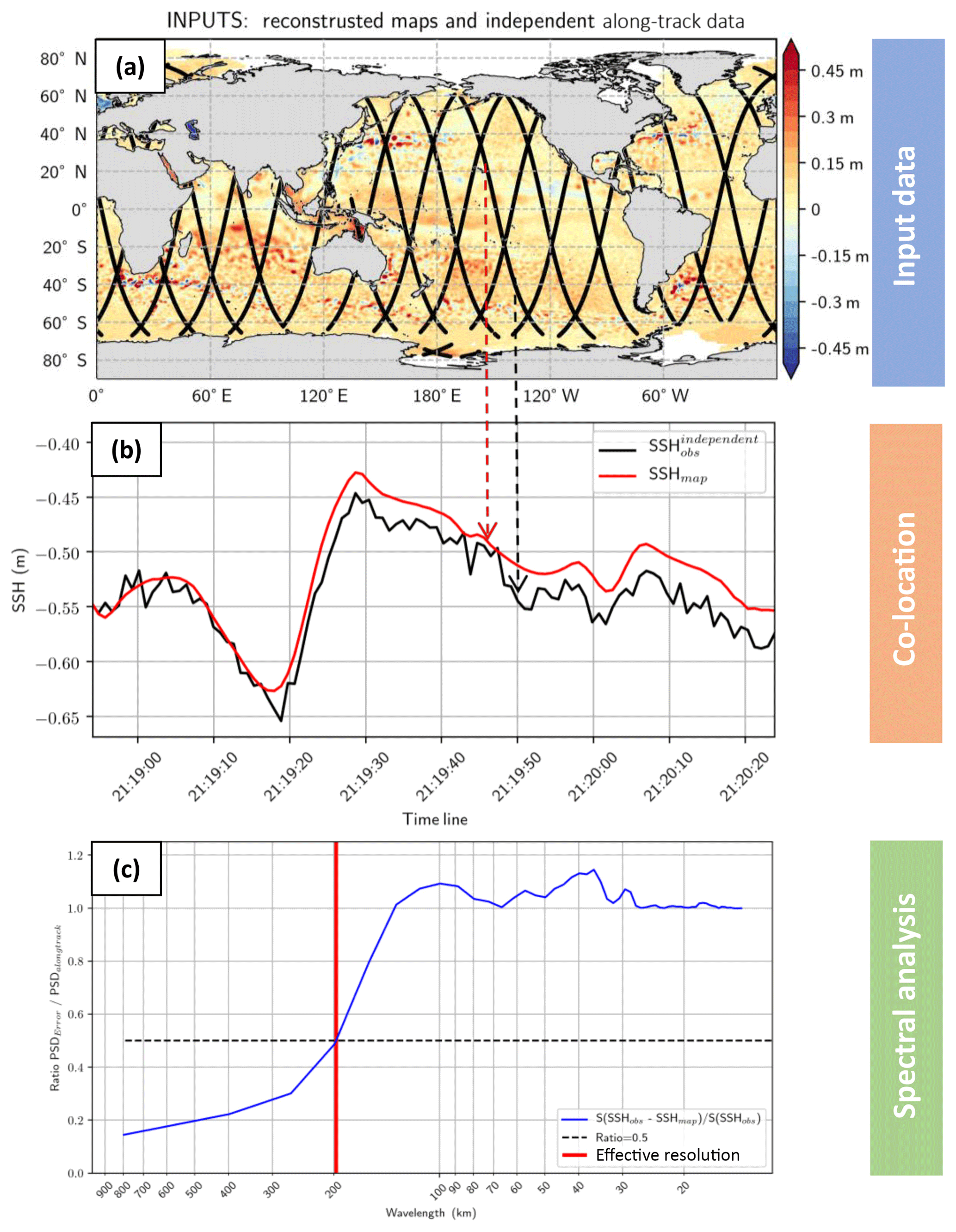
Figure 1 Schematic illustration of the methodology: (a) input data selection, (b) co-location of SLA and gridded SLA and (c) spectral analysis showing the ratio error spectrum to signal spectrum.

A comparison of SLA maps with an independent tide gauge dataset is carried out to estimate the effective temporal resolution. The approach is like the estimate of the effective spatial resolution and based on the computation of the ratio between the spectral content of the mapping error and the spectral content of the true tide gauge signal (Eq. 2):

$$\begin{array}{}\text{(2)}& \mathrm{NSR}\left({\mathit{\lambda }}_{\mathrm{t}}\right)={\displaystyle \frac{S_{\mathrm{diff}}\left({\mathit{\lambda }}_{\mathrm{t}}\right)}{S_{\mathrm{obs}}\left({\mathit{\lambda }}_{\mathrm{t}}\right)}},\end{array}$$

where λ_t is the temporal wavelength, S_diff(λ_t) is the power spectral density of the difference (SLA_obs–SLA_map) and S_obs(λ_t) is the spectral density of the independent observation.

We computed the effective temporal resolution from each tide gauge time series of the GLOSS-CLIVAR network. The temporal domain covers the period 1 January 1993–31 December 2015. The computation for each time series follows three main steps:

• At each tide gauge location, we extract the gridded SLA time series that is most highly correlated with tide gauge time series (note that the maximum distance separation of the grid point that is most highly correlated with each tide gauge is 100 km on average and can be as large as 300 km)

• Each highly correlated time series (based on correlation criterion > 0.8) is subsampled into 365 d segments to compute the spectral densities S_diff and S_obs. The length of each segment must be set when estimating power spectral density using Welch's method. By subsampling into 365 d segments, we limit the frequency range to only periods shorter than 365 d. Note that consideration of time series longer than 365 d reduced the number of realizations because of occasional gaps in some of the data records. This can have an impact on the local estimation of the effective temporal resolution, e.g., from 365 d to 2-year segments we lose some continuous time series that do not contain a ≥365 d segment. In these cases, the spectral analysis cannot be performed.

• The effective temporal resolution at each tide gauge location is given by the period λ_t where the ratio NSR(λ_t) is equal to 0.5 (deduced by linear interpolation between successive NSR values).

Note that this estimation of the temporal resolution is subject to an important caveat: the estimation is based mainly on coastal locations which may be contaminated by altimetry errors. Additionally, it may not be fully representative of the temporal resolution of the DUACS maps which combine various oceanic regimes (e.g., coastal, offshore high variability, offshore low variability regimes). Our results may therefore be crude but useful estimates of the temporal resolution.

We somewhat subjectively define the effective resolution to be the wavelength above which the NSR exceeds 0.5. In other words, it corresponds to the threshold where the mapping error variance is 2 times smaller than the observed true signal variance. The methodology used here is similar to that by Chelton et al. (2019), except that Chelton et al. (2019) consider the NSR in the spatial domain, whereas we here consider the NSR in the wavenumber domain. To illustrate and discuss the impact of the choice of the NSR criterion on the resolution, a sensitivity study is provided in Appendix B. We demonstrate that the resolution can be ∼30 % coarser with NSR = 0.25 (SNR = 4) and >30 % coarser with a more conservative NSR criterion (e.g., SNR = 10, as recommended by Chelton et al., 2019). It is worth mentioning that various approaches may exist to estimate the resolution (e.g., spectral magnitude ratio, filter transfer function). All measures of resolution have their advantages and drawbacks. We discuss in Appendix A the impact of using these different approaches in the estimation of the effective resolution.

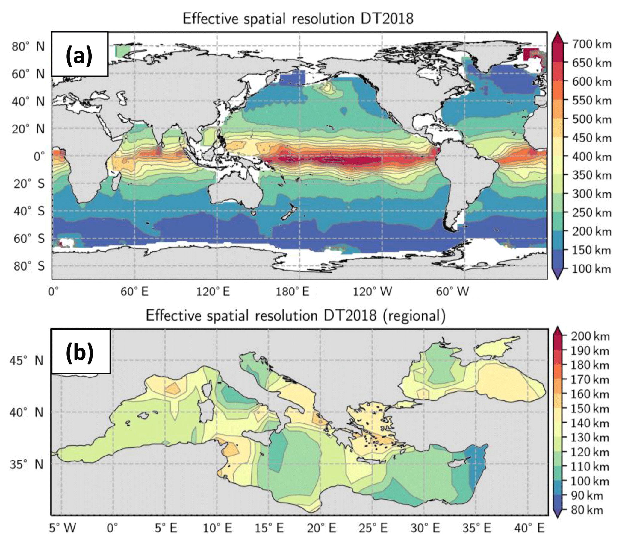
Figure 2 Effective spatial resolution, in kilometers, of the DUACS-DT2018 maps for (a) the Global Ocean product (b) the Mediterranean Sea and the Black Sea products; units in kilometers.

3 Results

3.1 Effective resolutions of the DUACS-DT2018 maps

The effective spatial resolution of the DUACS-DT2018 global maps is shown in Fig. 2a. Resolution was computed for maps constructed with three altimeters (CryoSat-2, HY-2, Jason-2) over the period 12 April 2014–31 December 2015 and Saral/AltiKa data were used as an independent dataset. We believe that this assessment of the spatial resolution based on maps constructed with three altimeter missions may be considered a reasonable averaged estimate since about three altimeter missions are used in the merging for the CMEMS products 70 % of the time over the period 1 January 1993–15 May 2017. The resolution ranges from ∼100 km wavelength at high latitudes to ∼800 km wavelength near the Equator, with a mean resolution at midlatitude near 200 km. Considering that eddy radius characteristic can be estimated as 20 %–25 % of the wavelength (Chelton et al., 2011, 2019), this means that ∼25 km radius structures are properly resolved in the maps at high latitudes, ∼200 km radius structures are resolved in the equatorial band and ∼50 km radius structures are resolved at midlatitudes. The effective spatial resolution of the DUACS-DT2018 Mediterranean Sea maps ranges from 90 to 160 km wavelength (Fig. 2b). The averaged resolution is ∼130 km wavelength over the basin. The effective spatial resolution of the DUACS-DT2018 Black Sea maps ranges from 100 to 150 km wavelength and the averaged resolution is ∼130 km wavelength over the basin (Fig. 2b).

The effective temporal resolution of the DUACS-DT2018 maps ranges from 2 to 140 d (Fig. 3). The temporal resolution is heterogeneously distributed over the global ocean, particularly in the intertropical band where a wide range of scales is found, linked to the mixture of continental tide gauges and island tide gauges, with the latter being more representative of open-ocean conditions. At mid-to-high latitudes the zonally averaged temporal scales are between 14 and 45 d, coherent with the temporal correlation scales applied in the mapping process. The globally averaged effective temporal resolution is estimated to be ∼34 d.

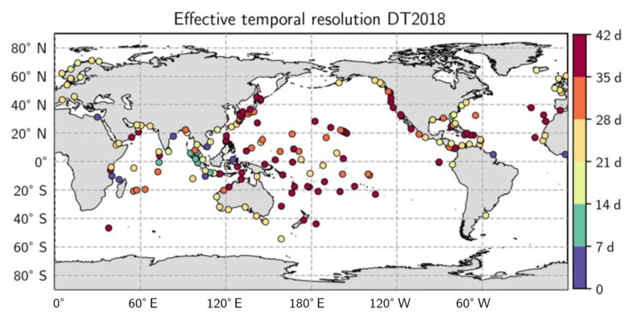
Figure 3 Effective temporal resolution in days of the DUACS-DT2018 maps. Unit in days.

The globally averaged resolutions of about 200 km by 34 d are consistent with the resolutions reported by Chelton et al. (2011, 2014) and Pujol et al. (2016). Using the spectral ratio method (see Appendix B), they found spatial resolution slightly better than 200 km at midlatitude in the Pacific Ocean.

3.2 Evolution of DUACS

We here investigate the impact of the DUACS upgrade from 2010 to 2018 to highlight the progress of the DUACS processing. Resolutions were computed for maps constructed with two altimeters (TOPEX/Poseidon and Jason-1) over the period 1 January 2003–31 December 2004 and Geosat Follow-On data were used as an independent dataset. To identify the impact of the DUACS upgrade, we computed the relative improvement or deterioration of the effective resolutions (expressed in percentage) for the upgrade DT2010 to DT2014, and DT2014 to DT2018 (Fig. 4). A negative (positive) value means finer (coarser) resolution with the upgrade. The comparison of the DT2010 and DT2014 processing shows finer resolution (improvement > 2 %) in DT2014 than in DT2010 in the high variability regions, e.g., the Gulf Stream system, the Kuroshio system and the Antarctic Circumpolar Current (ACC) (Fig. 4a). These improvements are associated with updated processing such as improved instrumental and atmospheric correction, tide correction, intercalibration method and smaller correlation scale in the mapping process. Coarser resolutions in DT2014 than in DT2010 are found in the equatorial band and are potentially linked to larger correlation scales applied in this region in the DT2014, as reported by Pujol et al. (2016). Although the DT2018 and DT2014 global maps have similar mean effective spatial resolution, regional investigation highlights ∼2 % to 10 % improved resolution in DT2018 in highly turbulent regions (Fig. 4b), such as the equatorial region, the Gulf Stream system, the Kuroshio system and some regions in the ACC. These improvements are linked to the new mapping standard (optimized selection of the observations in the turbulent region and a priori knowledge of the SLA variance based on a longer period in DT2018). The loss of resolution in the equatorial South Atlantic is not understood yet.

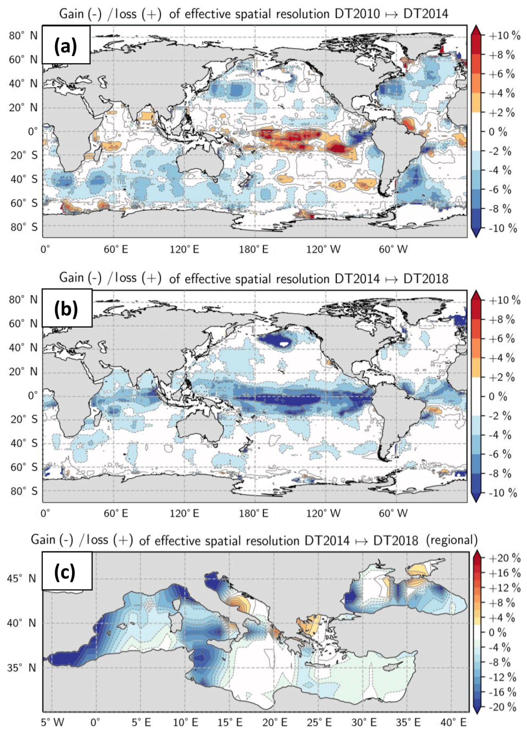
Figure 4 Gain/loss of effective spatial resolution for (a) the Global Ocean product between DT2014 and DT2010, (b) the Global Ocean product between DT2018 and DT2014 and (c) the Mediterranean Sea product and the Black Sea products between DT2018 and DT2014. Negative values mean that the resolution capability is finer. Note the different color bar scale between global and regional products.

Similar comparison is performed for the Mediterranean and Black Sea regional products focusing on the upgrade DT2014 to DT2018. Resolutions were computed for regional DUACS maps constructed with three altimeters (Jason-2, CryoSat-2, HY-2) over the period 12 April 2014–31 December 2015 and Saral/AltiKa was used as an independent dataset. The resolution capability of the Mediterranean Sea maps is slightly finer (∼4 %) in DT2018 than in DT2014 (Fig. 4c). The largest improvements (>6 %) are found in the western Mediterranean basin. The resolution in DT2018 is slightly coarser in the closed seas (Adriatic Sea and Aegean Sea). In these regions, the limited number of along-track data restricts a reliable interpretation of the spectral signal (see Fig. A1). The resolution capability of the Black Sea maps is on average slightly finer (∼3 %) in DT2018 than in DT2014, although a deterioration is found in the central part of the basin, which is also linked to a reduced number of spectral computations (Fig. 4c).

The DUACS-DT2018 and the DUACS-DT2014 maps have mean effective temporal resolutions of ∼34 d and 37 d, respectively. The differences can be locally larger than 15 %, near 30^∘ along the Japanese coast (∼10 d gain), as shown in Fig. 5. In these regions, the temporal resolution in the DUACS-DT2018 is finer than in DUACS-DT2014. These regions also coincide with the largest increased correlation score in the DUACS-DT2018 between SLA time series from maps and from independent tide gauge sensors (Taburet et al., 2019). These coastal improvements are linked to the new altimeter standards in coastal regions in DT2018 (Taburet et al., 2019).

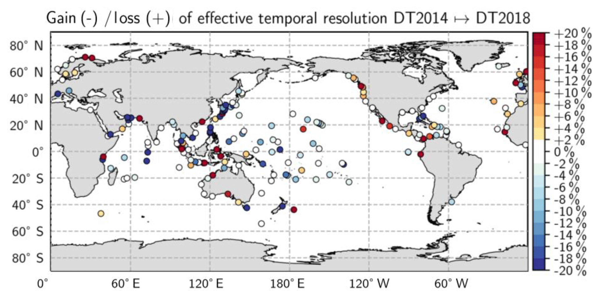
Figure 5 Gain/loss of effective temporal resolution between DT2018 and DT2014. Negative values mean that the resolution capability is better in DT2018 than DT2014.

3.3 Impact of altimeter constellation on the effective spatial resolution

Since the number of altimeter data processed by DUACS varies with time (according to the availability of satellites and the data quality), we investigated the impact of the constellation on the effective spatial resolution. Figure 6 illustrates the impact of the number of altimeters (two or three missions) used in the mapping on the effective spatial resolution. We verify, with our diagnostic, modest increases of resolving capabilities in the DUACS maps with increasing number of altimeters and found a globally averaged gain of resolution of ∼5 % from maps constructed with three altimeters compared with two altimeters. The resolution improvements may be considered modest. The reason is that the same covariance parameters are used in the optimal interpolation (OI) procedure regardless of how many altimeters are available. These OI parameters exert very strong constraints on the filter transfer function of the OI procedure.

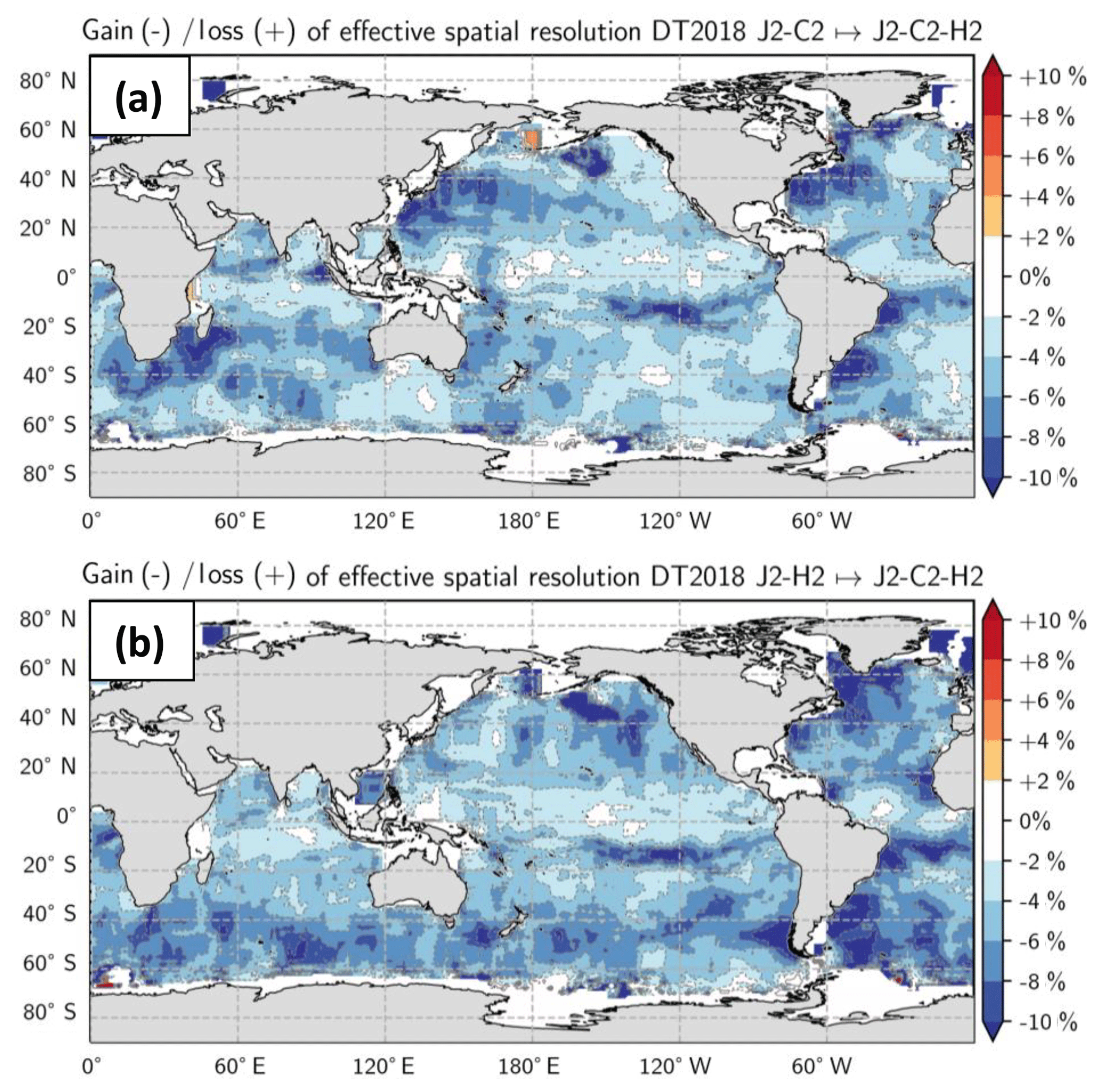
Figure 6 Impact of the satellite constellation on the effective resolution – ratio of effective resolution of (a) maps constructed with C2-H2-J2 vs. C2-J2 and (b) maps constructed with C2-H2-J2 vs. H2-J2.

Regional gains of resolution can be larger than 10 %. Additionally, it is possible to identify the improved resolving capability when a new mission is introduced into DUACS: for example, Fig. 6a illustrates the improved resolving capability when mission HY-2 is introduced into the mapping, Fig. 6b illustrates the improved resolving capability when mission CryoSat-2 is introduced in the mapping. It is shown that the major contribution of the HY-2 mission in the mapping is in the high variability regions (Gulf Stream, Kuroshio, Agulhas systems) while CryoSat-2 contributes in the mid-to-high-latitude regions. On the global scale, the distribution of the effective spatial resolution is shifted toward shorter scales when the number of missions used in the merging increases (Fig. 7) or when recent altimeters are used in the interpolation (e.g., compare the resolution maps from DT2018 constructed with historical Jason-1/Envisat vs. the maps from DT2018 constructed with currently operational missions Jason2/HY-2 or Jason-2/CryoSat2).

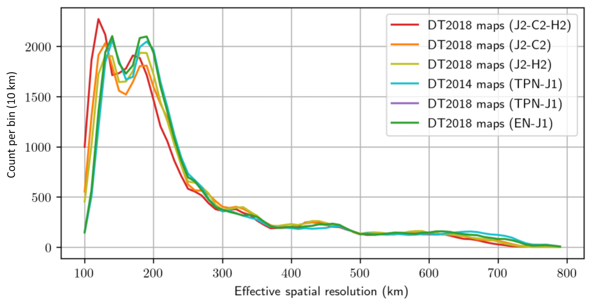
Figure 7 Distribution of the effective spatial resolution for various altimeter merging configuration.

4 Discussion and conclusions

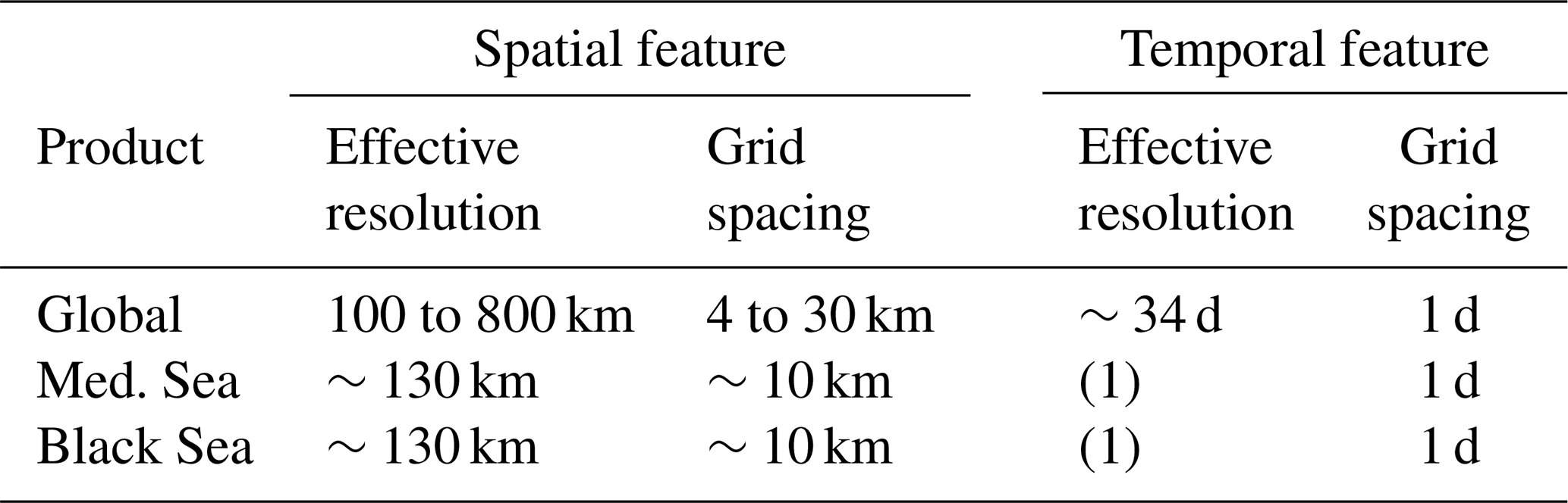
The present study investigates the resolving capability of the DUACS delayed-time gridded products (Global, Mediterranean Sea and Black Sea) delivered through the CMEMS catalogue. The key results are summarized in Table 1. Our method is based on the noise-to-signal spectral ratio to estimate the resolution. While along-track altimeter data resolve wavelength scales on the order of a few tens of kilometers (Dussurget et al., 2011; Dufau et al., 2016), we found that the merging of these along-track data into continuous maps in time and space leads to properly resolved structures with a wavelength scale of 100 km (a feature radius scale of ∼25 km) at high latitudes to 800 km (a feature radius scale of ∼200 km) near the Equator in the global gridded product and with a temporal scale of about 34 d. The same analysis applied to the regional Mediterranean Sea and Black Sea products showed resolving capability of structure with feature radius resolution of ∼30 km, which corresponds to ∼3 points grid spacing.

Table 1 Summary of the DUACS products spatial and temporal resolutions. (1) Not estimated due to the limited amount of tide gauges in the Mediterranean Sea and Black Sea.

These results are consistent with previous investigations. Based on a spectral ratio approach (cf. Appendix B), Chelton et al. (2011) estimated a wavelength resolution of ∼200 km for DT2010 and Chelton et al. (2014) estimated a wavelength resolution of ∼180 km for DT2014 in the midlatitude Pacific Ocean. Our analysis, based on the DT2018 global maps, suggests a wavelength resolution of ∼200 km at midlatitudes. As illustrated in Fig. 8, we verified that our estimation of the zonally averaged feature radius resolution of the mesoscale structures that can be properly mapped is smaller than the eddy scales computed by Chelton et al. (2011). The eddy length scales range from ∼70 km at high latitudes to ∼180 km near the Equator. The effective resolution is ∼1.6 times smaller than the eddy length scale. Additionally, we confirm that the minimum 4-week lifetime criteria used by Chelton et al. (2011) to identify and follow eddies seems to be compatible with the 34 d resolution capability. Note that our timescale estimation is based mainly on coastal locations and might not be representative of all oceanic regimes.

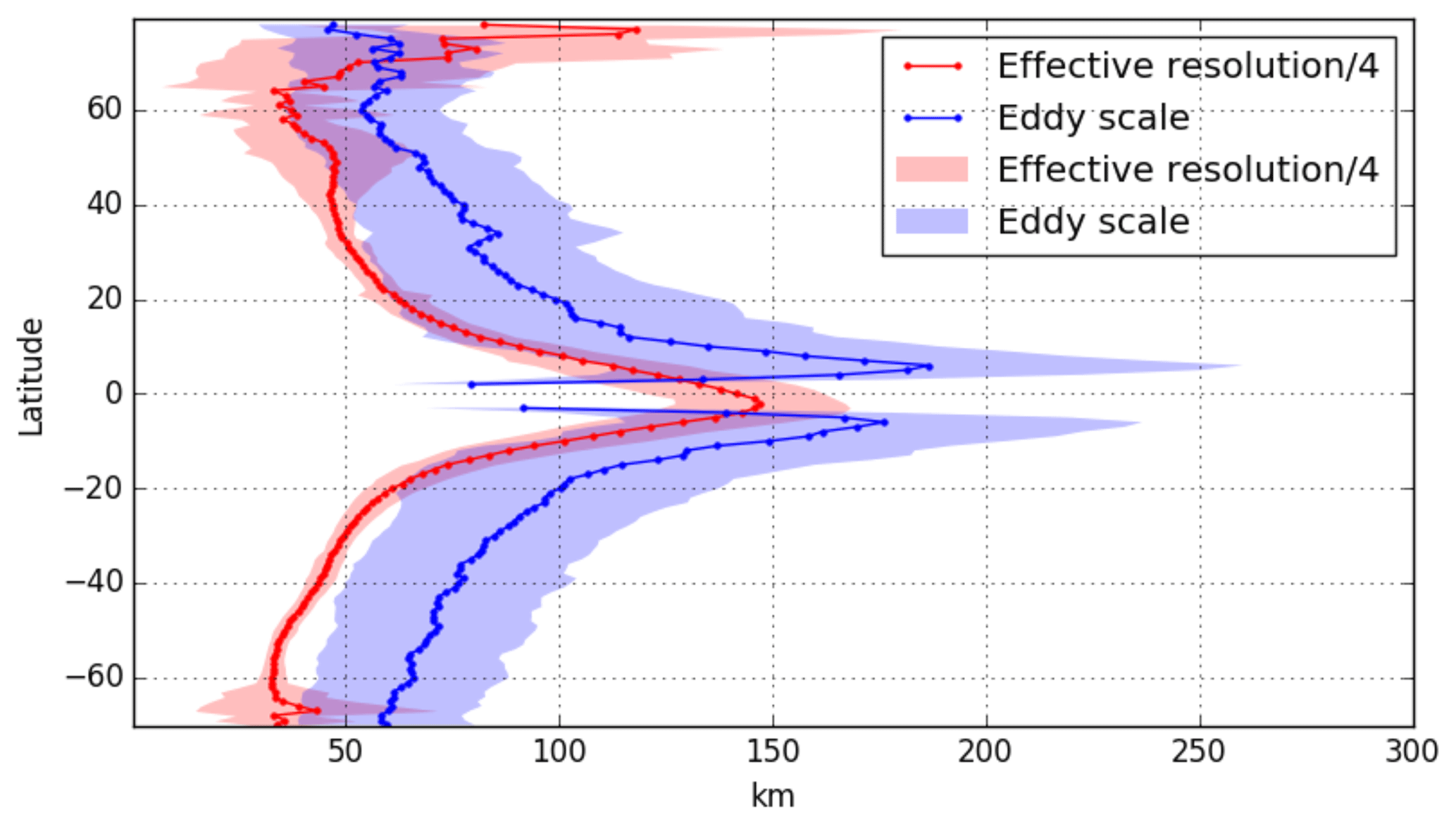
Figure 8 Zonally averaged eddy scale (as in Chelton et al., 2011; and computed from the DUACS-DT2018 two satellites maps) and feature radius resolution of the mesoscale structures that can be properly mapped in DUACS (i.e., derived as 0.25 × effective resolution). Units in kilometers.

The comparison of the DUACS-DT2018 reprocessing with former DUACS reprocessing (DT2010 and DT2014) reveals that finer structures are mapped in the global and regional Mediterranean Sea DT2018 products. For the Black Sea product, the interpretation is more complex due to the small dimension of the basin and the limited amount of spectral computation. Globally, we found that the largest improvements reach 20 % and are mainly in high variability regions, associated with the new mapping standard (e.g., optimized selection of the along-track data, new a priori knowledge of the signal variance based on 25 years of altimetry data, updated correlation scales for the regional Mediterranean Sea product) and new altimeter standards (e.g., instrumental and atmospheric corrections, tide corrections, intercalibration method). The improvement patterns between DT2014 and DT2010 global maps are similar to those found by Pujol et al. (2016) using statistical comparison between maps and independent along-track, and drifter, datasets. The improvement patterns between DT2018 and DT2014 global maps coincide with those found by Taburet el al. (2019) for the validation of the DT2018 products. Using statistical comparison between maps and independent along-track altimeter data, Taburet et al. (2019) also found improvement (∼3 %–4 %) of the mapped mesoscale structures in the high variability region and in the western Mediterranean Sea basin. Note that, at global scale, Taburet et al. (2019) diagnosed the largest improvements between DT2018 and DT2014 in the coastal regions which are partially edited (along 100 km coastal band) in the processing for estimating the spatial scale in this study, but they are detected with the temporal scale analysis showing shorter timescale in the DT2018 compared with DT2014.

Several studies showed that at least two altimeters are required to accurately map the SSH mesoscale structures (Le Traon and Dibarboure, 1999; Ducet et al., 2000; Pujol and Larnicol, 2005; Dibarboure et al., 2011; Chelton et al., 2007, 2011) and up to four altimeters are required for near-real-time products (Pascual et al., 2006) because only past observations are available for the mapping. This reduced number of observations has an impact on the estimation of the sea surface height. The present study reinforces these findings, showing that the resolution capability increased ∼10 %–20 % at regional scale from the merging of data from two to three altimeters.

It is worth noting that we probably underestimate the resolution capability of the maps since we are estimating the spatial effective resolution of degraded maps to keep an independent dataset aside. The resolution might hence be somewhat finer in the distributed CMEMS products. Although the satellite constellation ranges from 1 to 5 altimeter(s) between 1 January 1993 and 15 May 2017, we believe that our estimation of the spatial resolution based on maps constructed with three altimeter missions may be considered a reasonable averaged estimate since about three altimeter missions are used in the merging for the CMEMS products 70 % of the time over the period 1 January 1993–15 May 2017. We can expect >5 % finer resolution over the period where more than four altimeters are available (i.e., recent period). Likewise, we can expect on average 5 % coarser resolution when only two altimeters are available.

To conclude, the number and the quality of altimeters simultaneously operational, the along-track configuration and sampling pattern, the weight given to the altimeter data in the mapping procedure, and the choice of threshold SNR are key factors controlling the resolution capability of the DUACS gridded products. One may expect that in permitting to observe finer mesoscale or sub-mesoscale structures (Dufau et al., 2016; Pujol et al., 2012), future instrumental systems based on large-swath altimeters (such as Surface Ocean and Water Topography – SWOT) combined with new mapping techniques based on dynamic interpolation (Ubelmann et al., 2016) will push the resolution of maps toward new limits.

Appendix A: Other approach to estimate the resolution

A1 Spectral magnitude ratio

Chelton et al. (2011, 2014) estimated the resolution of the DUACS-DT2014 maps based on the calculation of the spectral magnitude ratio between the reference Stammer (1997) along-track spectrum and gridded SSH spectra. Similarly, we here estimate the resolution based on the spectral ratio between independent along-track and gridded SSH signals (Eq. A1). It is defined as follows:

$$\begin{array}{}\text{(A1)}& \mathrm{SR}\left({\mathit{\lambda }}_{\mathrm{s}}\right)={\displaystyle \frac{S_{\mathrm{map}}\left({\mathit{\lambda }}_{\mathrm{s}}\right)}{S_{\mathrm{obs}}\left({\mathit{\lambda }}_{\mathrm{s}}\right)}},\end{array}$$

where S_obs(λ_s) denotes the power spectral density of the independent SSH along-track, S_map(λ_s) denotes the power spectral density of the SSH map interpolated onto the independent along-track segment, SR the spectral ratio and λ_s the wavelength. The resolution is given by the wavelength λ_s where the spectral ratio is equal to 0.5 and is based on the conventional notion of a filter being characterized by its half-power filter cutoff wavelength (Chelton et al., 2011). To differentiate it from the effective resolution, we named it useful resolution: useful for verifying the available and realistic amount of energy at a specific wavelength between two signals without considering their phase (e.g., useful for model sensitivity study).

Chelton et al. (2011, 2014) estimated the resolution of the DUACS-DT2010 and DUACS-DT2014 as the wavenumber at which the power is a factor of 2 smaller than the Stammer (1997) spectrum. From their analysis, they estimated a spatial resolution of ∼2^∘ for the DUACS-DT2010 and ∼1.7^∘ for the DUACS-2014. Chelton et al. (2014) found essentially the same resolution between maps constructed with two or four satellites.

The resolution estimated with the SR method is shown in Fig. A2a and the difference between the effective and useful resolutions is shown in Fig. A2b. The useful resolution of the DUACS-DT2018 maps ranges from 100 km at high latitude to 500 km near the Equator. The ratio of effective to useful resolution suggests somewhat finer resolution in the intertropical band using the SR approach and somewhat finer resolution at high latitude with the NSR approach. In other words, the amplitude of the mapped SSH spectral content is better in the intertropical band than the phase, whereas it is the opposite at high latitude. This feature highlights the difficulty to properly map propagating equatorial waves in DUACS. The two methods are equivalent at midlatitudes.

A2 Transfer function

The transfer function (H) measures the filtering properties of a system (Eq. A2). It is defined as follows:

$$\begin{array}{}\text{(A2)}& H\left({\mathit{\lambda }}_{\mathrm{s}}\right)={\displaystyle \frac{{\mathrm{CS}}_{\mathrm{obs}\text{-}\mathrm{map}}\left({\mathit{\lambda }}_{\mathrm{s}}\right)}{S_{\mathrm{obs}}\left({\mathit{\lambda }}_{\mathrm{s}}\right)}},\end{array}$$

where CS_obs-map(λ_s) is the cross-spectral density between the along-track data and the map interpolated onto the along-track segment and S_obs(λ_s) is the power spectral density of the along-track. Note that in this case, the along-track data are considered nonindependent (i.e., they are used in the mapping system). The resolution is given by the wavelength λ_s where H is equal to 0.5. It is the same definition used by Schlax and Chelton (1992) to estimate the resolution capability of an arbitrarily sampled dataset.

The resolution estimated with the transfer function method is shown in Fig. A3a and the difference between the effective resolution and the transfer function resolution is shown in Fig. A3b. The transfer function resolution of the DUACS-DT2018 maps ranges from 100 km at high latitude to 400 km near the Equator. The difference between effective resolution vs. transfer function resolution suggests somewhat finer resolution using the transfer function. This is directly linked to the fact that the along-track data are here nonindependent. The assessment is undertaken below the track that is used in the filtering system. This diagnostic gives the filtering property of the system but suffers from nonindependency of the along-track dataset. The resolution may be different off-track.

These methods share the same number of spectrum calculation and number of segments used in the calculation (see Fig. A1) and each method has advantages and drawbacks. The spectral magnitude ratio compares the amplitude of the signals and the transfer function estimates the filtering properties from assimilated along-track data. The functions NSR(λ_s), SR(λ_s) and H(λ_s) are shown for location (45^∘ N, 330^∘ E) in Fig. A4. At this location, each function has a transition between 100 and 200 km wavelength, separating the high mapping error regime for wavelength < 100 km to the low mapping error for wavelength > 200 km (Fig. A4a), separating the high amplitude error regime for wavelength < 100 km to the low amplitude error for wavelength > 200 km (Fig. A4b), and separating the filter regimes (Fig. A4c).

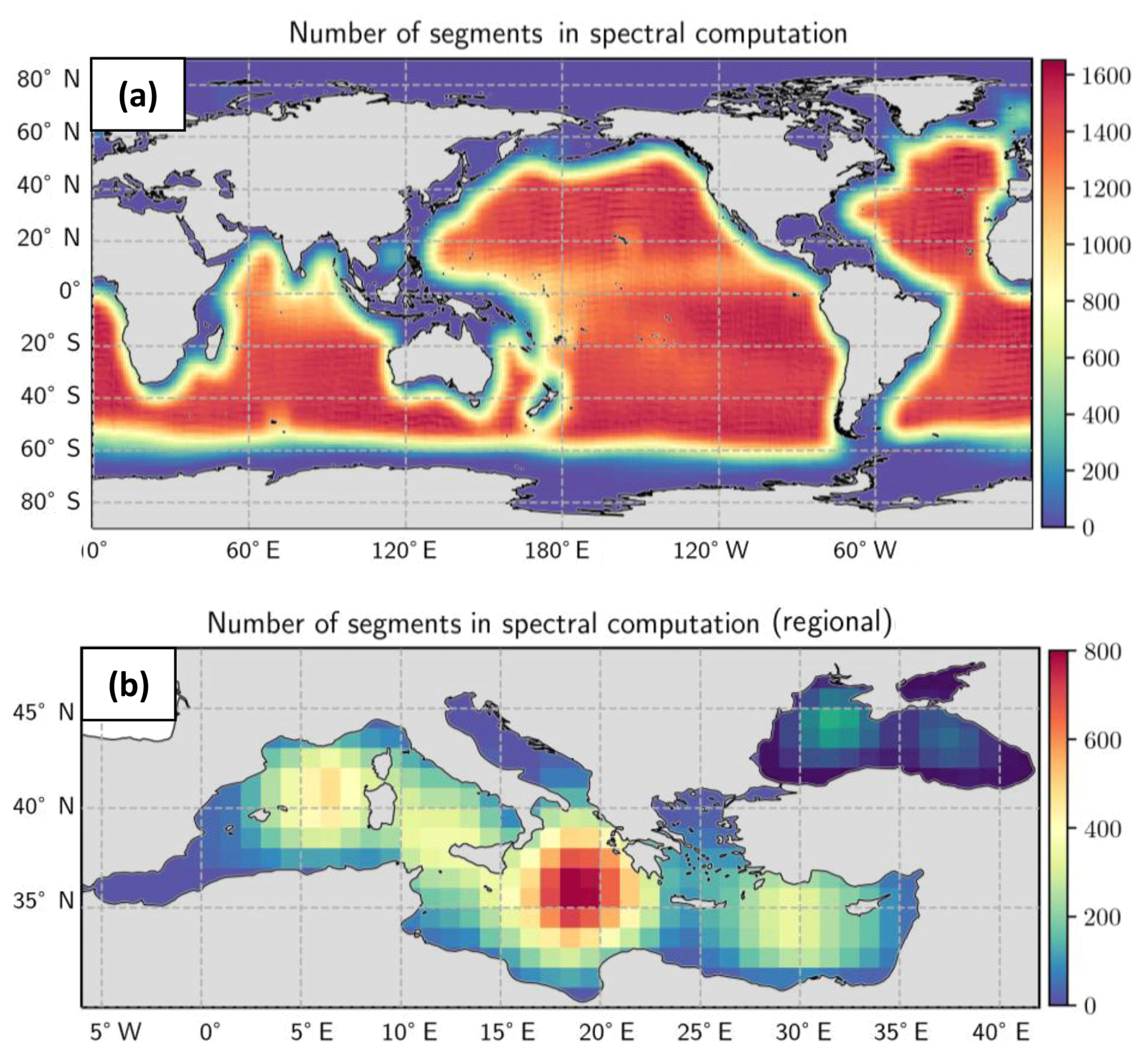
Figure A1 Number of segments used in the spectral computation for (a) the global product and (b) the regional Mediterranean and Black Sea products.

Figure A2 (a) DUACS-DT2018 useful resolution derived from spectral ratio (SR) approach and (b) ratio of effective to useful resolution for the DT2018 maps. Blue means finer resolution with NSR.

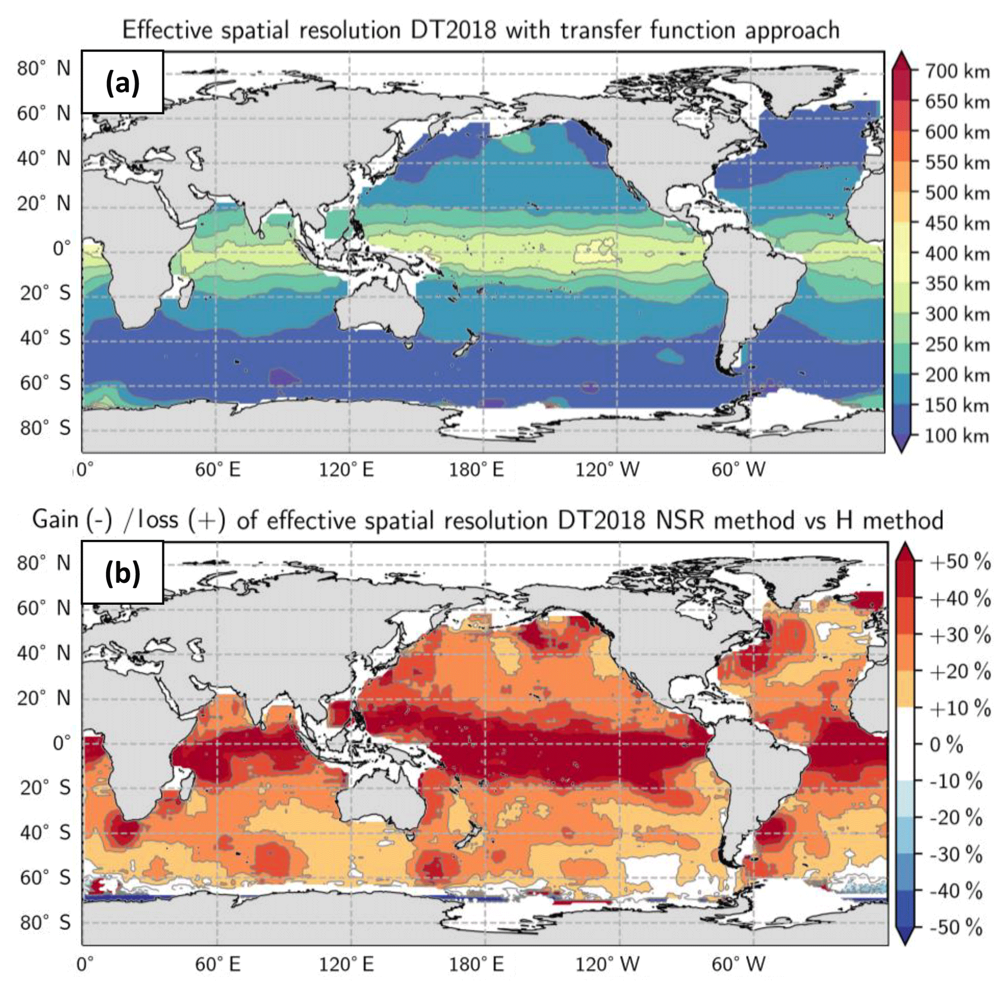
Figure A3 (a) DUACS-DT2018 resolution derived from the transfer function approach and (b) ratio of effective to transfer function resolution for the DT2018 maps. Blue means finer resolution with NSR.

Figure A4 Illustration of the various spectral functions used to estimate the resolution at 45^∘ N, 330^∘ E: (a) with NSR method, (b) with SR method and (c) with the transfer function (H).

Appendix B: Sensitivity of the noise-to-signal ratio (NSR) criterion

We here investigate and discuss the impact of the NSR criterion on the estimation of the effective resolution. NSR criterion is used to define the resolution limit of the map. In the present study, we choose the NSR = 0.5 criterion to define the resolution limit. This value may be considered too generous; therefore, we present below the effective resolution for three cases, motivated by the analysis performed in the spatial domain by Chelton et al. (2019):

• criterion of NSR = 0.5,

• criterion of NSR = 0.25,

• criterion of NSR = 0.1.

Figure B1a represents the effective resolution using NSR = 0.5 (SNR = 2) criterion, Fig. B1b using NSR = 0.25 (SNR = 4) criterion and Fig. B1c NSR = 0.1 (SNR = 10). For each panel the resolution becomes finer poleward. The white areas correspond to the regions where the NSR threshold criterion is not achieved. These areas become larger in the intertropical region as well as at high latitudes when the NSR criterion decreases. For NSR = 0.1, the resolution in the intertropical band cannot be computed with the method since the NSR is above 0.1 for all scales. To further illustrate this, we show an example of NSR at one specific point (lat = 16^∘ S, long = 346^∘ E) in Fig. B2. The analysis shows that the NSR is greater than 0.3 (i.e., SNR < 3) in this location. This large-scale low coherency between maps and along-track may be linked to the misrepresentation of the large-scale and rapid equatorial waves (e.g., equatorial gravity waves) in the mapping process, which are filtered in the mapping process.

Despite the areas of missing values in Fig. B1b and c, we quantify the difference in effective resolution between criterion NSR = 0.4 and NSR = 0.25 (Fig. B3) and NSR = 0.5 and NSR = 0.1. The difference between effective resolution computed with NSR = 0.5 vs. NSR = 0.25 is <30 % (∼60 km) at midlatitude and $<=\mathrm{50}$ % (400 km) in the intertropical band. The difference between effective resolution computed with NSR = 0.5 vs. NSR = 0.1 is <50 % (∼100 km) at midlatitude and >50 % in the intertropical band.

In conclusion, we here demonstrate that the choice of the NSR criterion has an impact on the estimation of the resolution. Setting a more conservative criterion of NSR = 0.25 leads to ∼30 % coarser effective resolution. The strongly conservative criterion NSR = 0.1 also reveals one of the major caveats in the DUACS maps processing: the poor representation of the large-scale and rapid equatorial circulation. This issue should be addressed in a future version of DUACS maps.

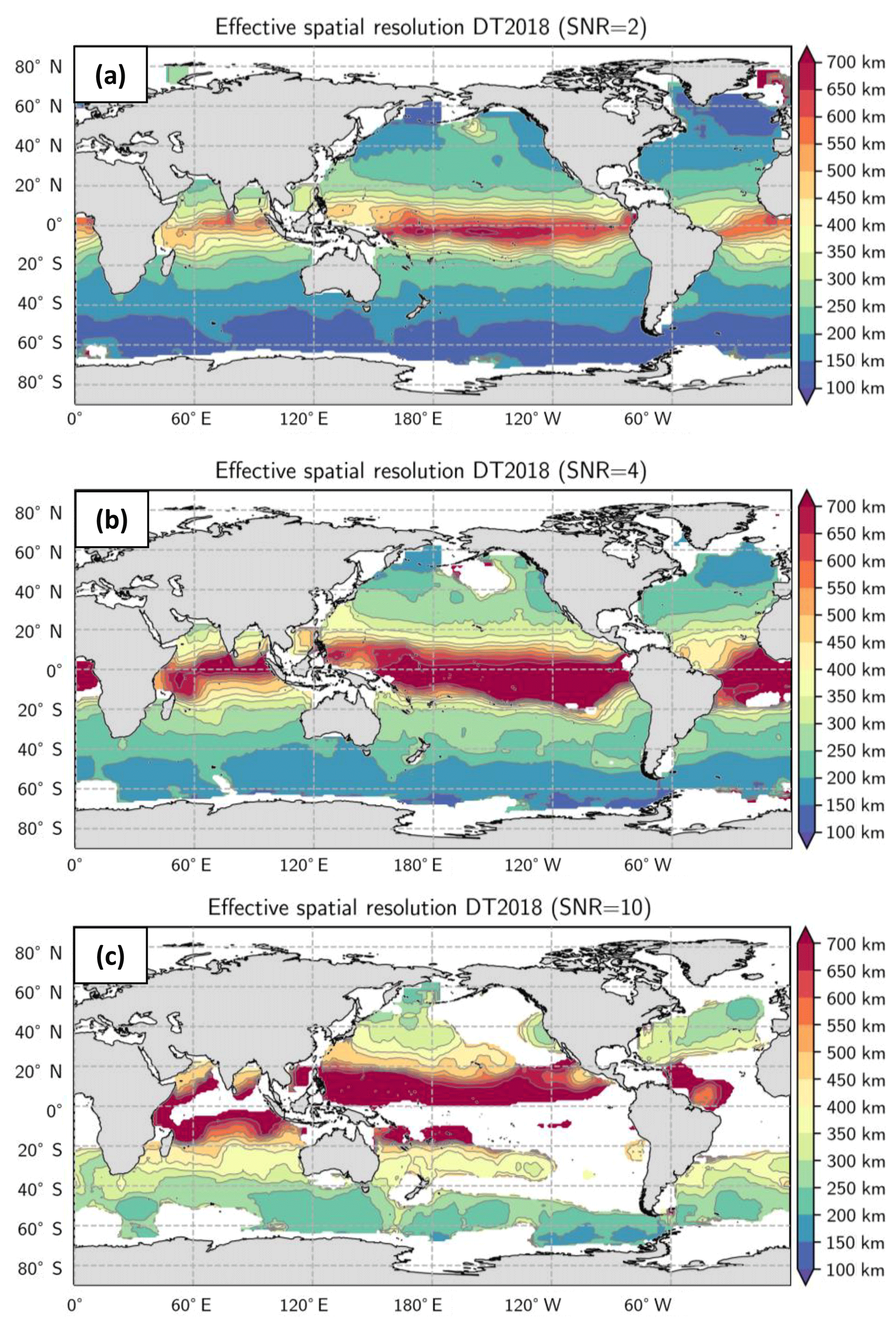
Figure B1 Effective resolution computed for three different SNR criteria: (a) SNR = 2, (b) SNR = 4 and (c) SNR = 10. The white areas correspond to the regions where the SNR threshold criterion is not achieved.

Figure B2 Ratio of NSR at longitude 346^∘ E and latitude 16^∘ S. We illustrate that the ratio at this location is always above >0.3 and so the resolution cannot be computed for SNR criterion > 4 (i.e., NSR < 0.25).

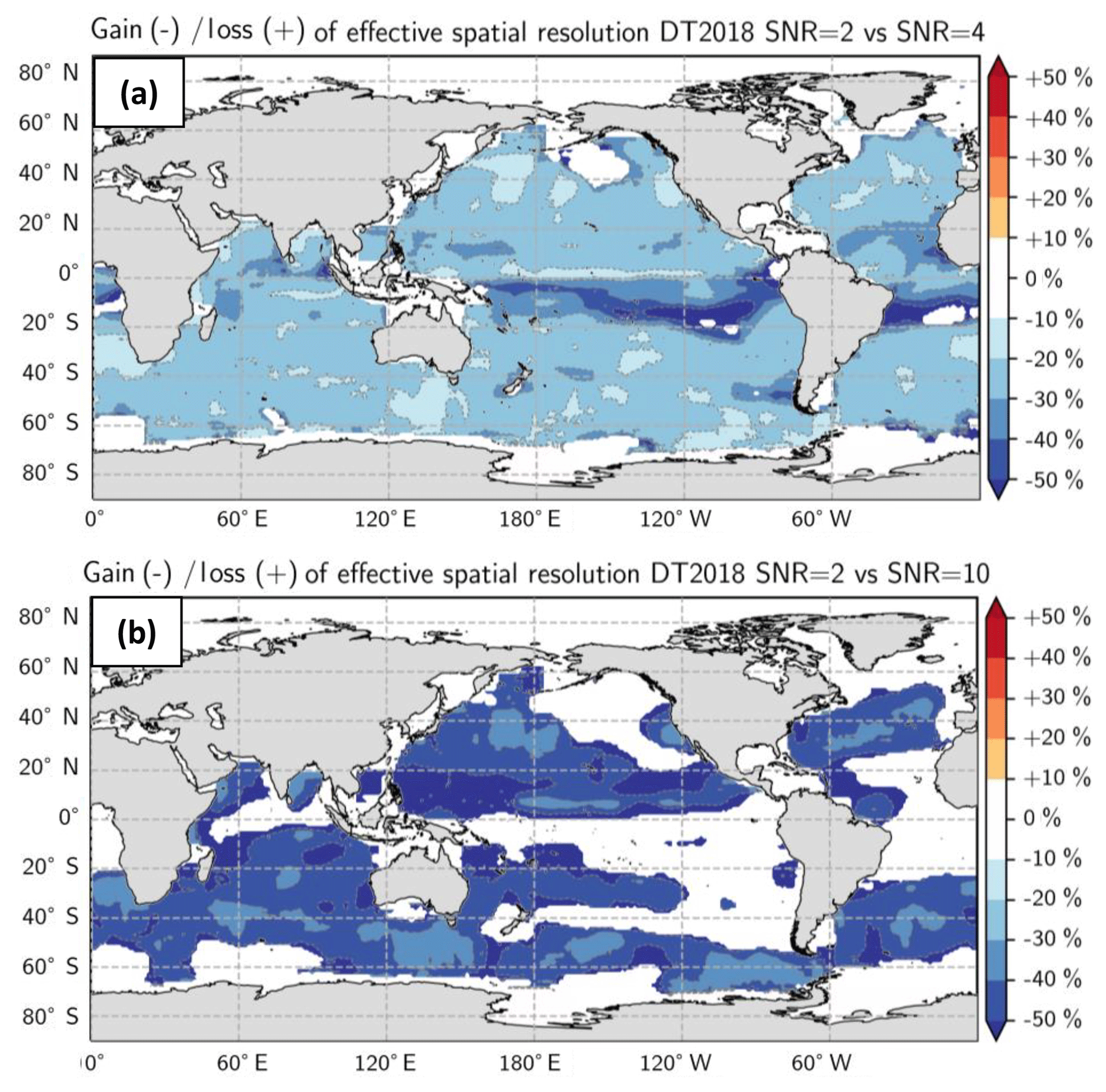
Figure B3 Ratio of effective resolution computed with (a) SNR = 2 vs. SNR = 4 criterion and (b) SNR = 2 vs. SNR = 10 criterion. Blue means finer resolution with SNR = 2. The white areas correspond to the regions where the SNR threshold criterion is not achieved.