Technical note: Two types of absolute dynamic ocean topography

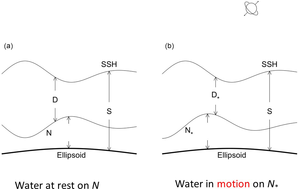
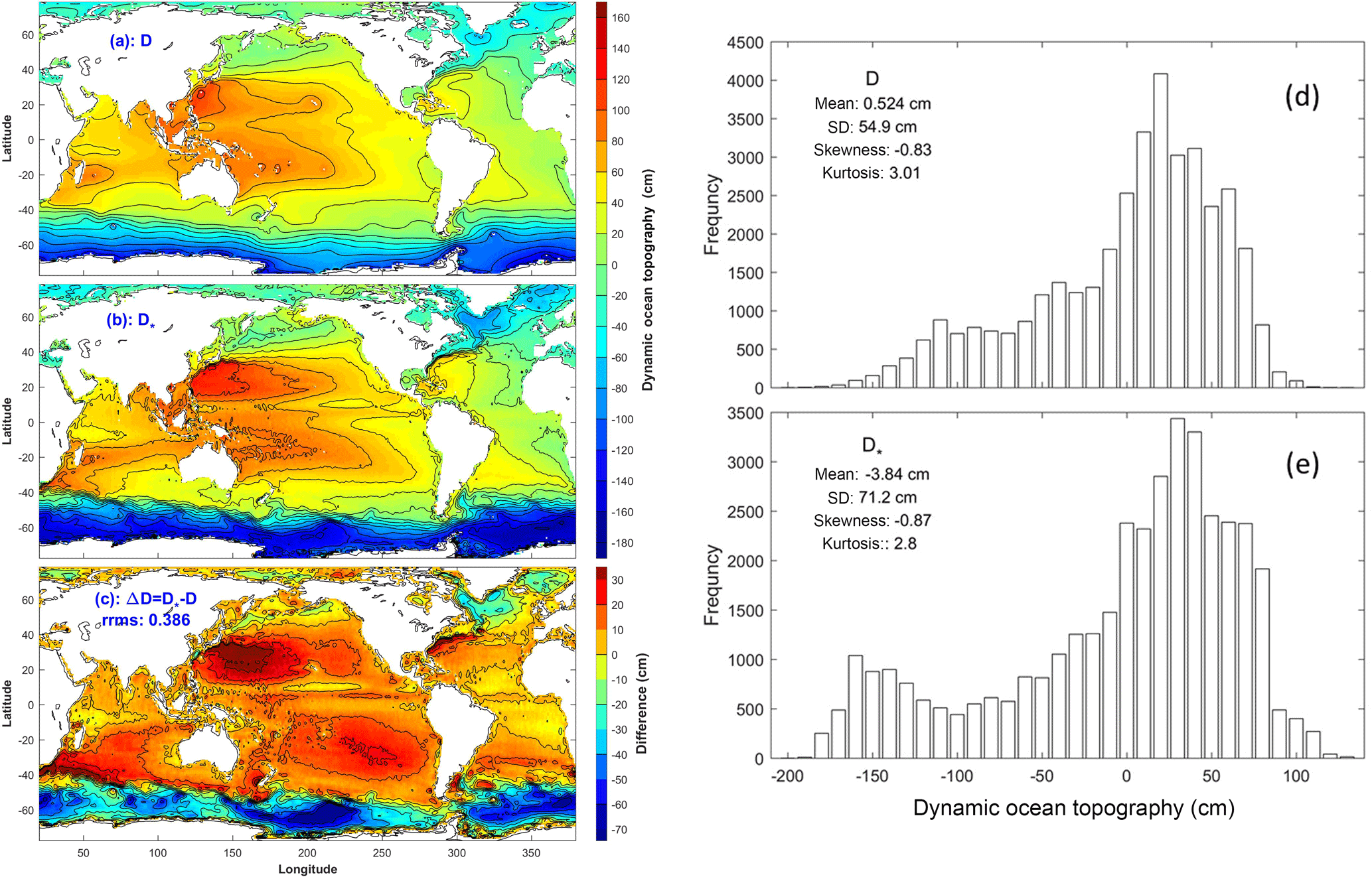
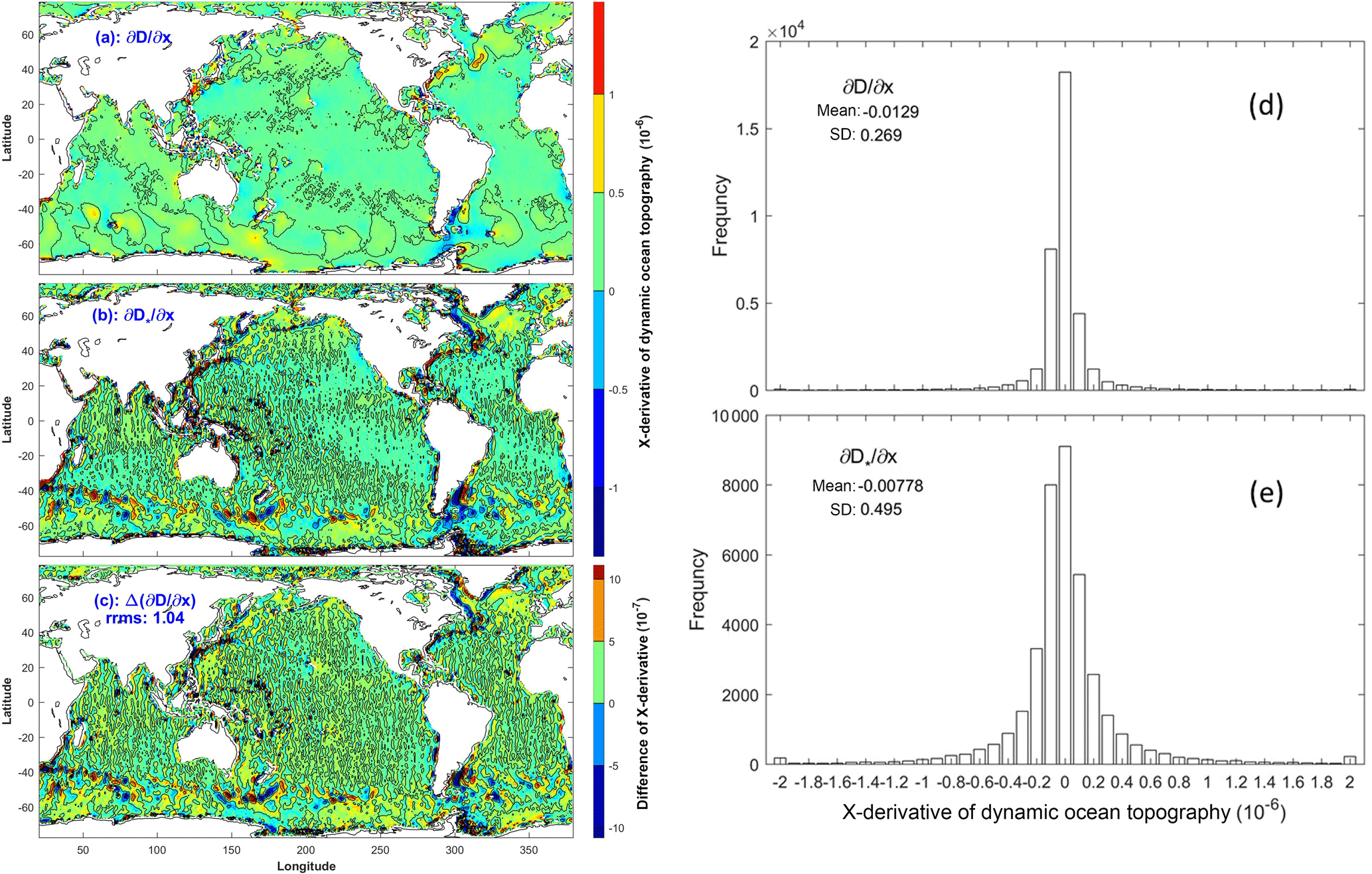
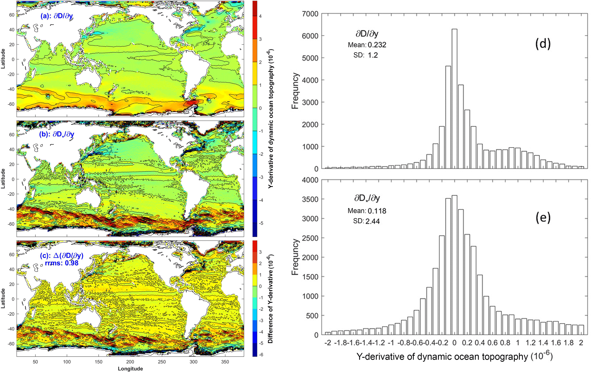
Two types of marine geoid exist with the first type being the average level of sea surface height (SSH) if the water is at rest (classical definition), and the second type being satellite-determined with the condition that the water is usually not at rest. The differences between the two are exclusion (inclusion) of the gravity anomaly and non-measurable (measurable) in the first (second) type. The associated absolute dynamic ocean topography (referred to as DOT), i.e., SSH minus marine geoid, correspondingly also has two types. Horizontal gradients of the first type of DOT represent the absolute surface geostrophic currents due to water being at rest on the first type of marine geoid. Horizontal gradients of the second type of DOT represent the surface geostrophic currents relative to flow on the second type of marine geoid. Difference between the two is quantitatively identified in this technical note through comparison between the first type of DOT and the mean second type of DOT (MDOT). The first type of DOT is determined by a physical principle that the geostrophic balance takes the minimum energy state. Based on that, a new elliptic equation is derived for the first type of DOT. The continuation of geoid from land to ocean leads to an inhomogeneous Dirichlet boundary condition with the boundary values taking the satellite-observed second type of MDOT. This well-posed elliptic equation is integrated numerically on 1^∘ grids for the world oceans with the forcing function computed from the World Ocean Atlas (T, S) fields and the sea-floor topography obtained from the ETOPO5 model of NOAA. Between the first type of DOT and the second type of MDOT, the relative root-mean square (RRMS) difference (versus RMS of the first type of DOT) is 38.6 % and the RMS difference in the horizontal gradients (versus RMS of the horizontal gradient of the first type of DOT) is near 100 %. The standard deviation of horizontal gradients is nearly twice larger for the second type (satellite-determined marine geoid with gravity anomaly) than for the first type (geostrophic balance without gravity anomaly). Such a difference needs further attention from oceanographic and geodetic communities, especially the oceanographic representation of the horizontal gradients of the second type of MDOT (not the absolute surface geostrophic currents).

1 Introduction

Let the coordinates (x, y, z) be in zonal, latitudinal, and vertical directions. The absolute dynamic ocean topography (hereafter referred to as DOT) $\widehat{D}$ is the sea surface height (SSH, waves and tides filtered out) relative to the marine geoid (i.e., the equipotential surface),

$$\begin{array}{}\text{(1)}& \widehat{D}=S-\widehat{N},\end{array}$$

where S is the SSH; $\widehat{N}$ is the marine geoid height above the reference ellipsoid (Fig. 1). $\widehat{D}$ is an important signal in oceanography and $\widehat{N}$ is of prime interest in geodesy. Equation (1) is also applicable if defined relative to the center of the Earth. The geoid height $\widehat{N}(x,y)$ and other associated measurable quantities such as gravity anomaly Δg(x, y) are related to the anomaly of the gravitational potential V(x, y, z) to a first approximation by the well-known Brun's formula (e.g., Hofmann-Wellenhof and Moritz, 2005),

$$\begin{array}{}\text{(2)}& \widehat{N}(x,y)={\displaystyle \frac{V(x,y,\mathrm{0})}{g}},\end{array}$$

where g=9.81 m s⁻², is the globally mean normal gravity, which is usually represented by g₀ in geodesy. The gravity anomaly is the vertical derivative of the potential

$$\begin{array}{}\text{(3)}& \mathrm{\Delta }g(x,y)=-{\displaystyle \frac{\partial V(x,y,\mathrm{0})}{\partial z}},\end{array}$$

where the anomaly of the gravity potential V satisfies the Laplace equation

$$\begin{array}{}\text{(4)}& {\displaystyle \frac{{\partial }^{\mathrm{2}}V}{\partial x^{\mathrm{2}}}}+{\displaystyle \frac{{\partial }^{\mathrm{2}}V}{\partial y^{\mathrm{2}}}}+{\displaystyle \frac{{\partial }^{\mathrm{2}}V}{\partial z^{\mathrm{2}}}}=\mathrm{0}.\end{array}$$

Figure 1 Two types of marine geoid and DOT: (a) the first type with N being the average level of SSH if water is at rest (classical definition), and (b) represents the second type with satellite-determined N_∗ (water in motion on N_∗).

The vertical deflection is the slope of the geoid

$$\begin{array}{}\text{(5)}& {\displaystyle \frac{\partial \widehat{N}}{\partial x}}={\displaystyle \frac{\mathrm{1}}{g}}{\displaystyle \frac{\partial V}{\partial x}},{\displaystyle \frac{\partial \widehat{N}}{\partial y}}={\displaystyle \frac{\mathrm{1}}{g}}{\displaystyle \frac{\partial V}{\partial y}},\end{array}$$

which connects to the gravity anomaly by

$$\begin{array}{}\text{(6)}& {\displaystyle \frac{\partial \left(\mathrm{\Delta }g\right)}{\partial z}}=g\left({\displaystyle \frac{{\partial }^{\mathrm{2}}\widehat{N}}{\partial x^{\mathrm{2}}}}+{\displaystyle \frac{{\partial }^{\mathrm{2}}\widehat{N}}{\partial y^{\mathrm{2}}}}\right).\end{array}$$

Equation (6) links the vertical gravity gradient to the horizontal Laplacian of the marine geoid height $\widehat{N}$ and serves as the basic principle in the satellite marine geodesy. Since $\widehat{D}$ is the difference of the two large fields S and $\widehat{N}$ (2 orders of magnitude larger than $\widehat{D})$, it is extremely sensitive to any error in either S or $\widehat{N}$ – even a 1 % error in either field can lead to error in $\widehat{D}$ that is of the same order of magnitude as $\widehat{D}$ itself (Wunsch and Gaposchkin, 1980; Bingham et al., 2008).

Before satellites came into operation, S was measured from sparse surveying ships and tide gauge stations located along irregular local coastlines. However, $\widehat{N}$ was not easy to observe. Without satellite measurements, the marine geoid is defined as the average level of SSH if the water is at rest and denoted here by N, which is called the classical marine geoid (or first type of marine geoid, Fig. 1a). The first type of marine geoid can be taken as a stand-alone concept in oceanography since it is on the basis of the hypothesis (mean SSH when the water at rest) without using the gravity anomaly. In this framework, the geostrophic balance

$$\begin{array}{}\text{(7)}& u_{\mathrm{g}}=-{\displaystyle \frac{\mathrm{1}}{f\widehat{\mathit{\rho }}}}{\displaystyle \frac{\partial \widehat{p}}{\partial y}},v_{\mathrm{g}}={\displaystyle \frac{\mathrm{1}}{f\widehat{\mathit{\rho }}}}{\displaystyle \frac{\partial \widehat{p}}{\partial x}}\end{array}$$

and hydrostatic balance

$$\begin{array}{}\text{(8)}& {\displaystyle \frac{\partial \widehat{p}}{\partial z}}=-\widehat{\mathit{\rho }}g\end{array}$$

are used for large-scale (i.e., scale > 100 km) processes. Here (u_g, v_g) are geostrophic current components; f is the Coriolis parameter; ($\widehat{p}$, $\widehat{\mathit{\rho }})$ are in situ pressure and density, respectively, which can be decomposed into

$$\begin{array}{}\text{(9)}& \widehat{\mathit{\rho }}={\mathit{\rho }}_{\mathrm{0}}+\stackrel{\mathrm{‾}}{\mathit{\rho }}\left(z\right)+\mathit{\rho },\widehat{p}=-{\mathit{\rho }}_{\mathrm{0}}gz+\stackrel{\mathrm{‾}}{p}\left(z\right)+p.\end{array}$$

Here, ρ₀=1025 kg m⁻³ is the characteristic density; ($\stackrel{\mathrm{‾}}{\mathit{\rho }}$, $\stackrel{\mathrm{‾}}{p})$ are horizontally uniform with $\stackrel{\mathrm{‾}}{\mathit{\rho }}$ vertically increasing with depth (stable stratification)

$$\begin{array}{}\text{(10)}& \partial \stackrel{\mathrm{‾}}{\mathit{\rho }}/\partial z\equiv -{\mathit{\rho }}_{\mathrm{0}}\left(n\right(z){)}^{\mathrm{2}}/g,\end{array}$$

where n(z) is the buoyancy frequency (or called the Brunt–Vaisala frequency); (p, ρ) are anomalies of pressure and density. Near the ocean surface, it is common to use the characteristic density and corresponding pressure (p₀,ρ₀) to represent ($\widehat{p}$, $\widehat{\mathit{\rho }})$. Vertical integration of Eq. (8) from N to S after replacing ($\widehat{p}$, $\widehat{\mathit{\rho }})$ by (p₀,ρ₀) in Eqs. (7) and (8) leads to

$$\begin{array}{}\text{(11)}& u_{\mathrm{g}}\left(S\right)-u_{\mathrm{g}}\left(N\right)=-{\displaystyle \frac{g}{f}}{\displaystyle \frac{\partial D}{\partial y}},v_{\mathrm{g}}\left(S\right)-v_{\mathrm{g}}\left(N\right)={\displaystyle \frac{g}{f}}{\displaystyle \frac{\partial D}{\partial x}},\end{array}$$

where

$$\begin{array}{}\text{(12)}& D=S-N\end{array}$$

is the first type of DOT. Since the first type of marine geoid (N) is defined as the average level of SSH if the water is at rest,

$$\begin{array}{}\text{(13)}& u_{\mathrm{g}}\left(N\right)=\mathrm{0},v_{\mathrm{g}}\left(N\right)=\mathrm{0},\end{array}$$

the horizontal gradient of D represents the absolute surface geostrophic currents.

After satellites came into operation, SSH has been observed with uniquely sampled temporal and spatial resolutions by high-precision altimetry above a reference ellipsoid (not geoid; Fu and Haines, 2013). Two Gravity Recovery and Climate Experiment (GRACE) satellites, launched in 2002, provide data to compute the marine geoid (called the GRACE Gravity Model, GGM; see website: http://www.csr.utexas.edu/grace/ (last access: 31 July 2018); Tapley et al., 2003; Shum et al., 2011). In addition, the European Space Agency's GOCE mission data, along with the GRACE data, have produced the best mean gravity field or the geoid model at a spatial scale longer than 67 km half-wavelength (or spherical harmonics completed to degree 300). This marine geoid is the solution of Eq. (6),

$${\displaystyle \frac{{\partial }^{\mathrm{2}}{N}_{\ast }}{\partial x^{\mathrm{2}}}}+{\displaystyle \frac{{\partial }^{\mathrm{2}}{N}_{\ast }}{\partial y^{\mathrm{2}}}}={\displaystyle \frac{\mathrm{1}}{g}}{\displaystyle \frac{\partial \left(\mathrm{\Delta }g\right)}{\partial z}},$$

where N_∗ is the satellite-determined marine geoid from the measurable gravity anomaly Δg, and called the second type of marine geoid (Fig. 1b), which is different from N, defined by Eq. (13). Correspondingly, the second type of DOT is defined by

$$\begin{array}{}\text{(14)}& D_{\ast }=S-N_{\ast }\left(t\right),\end{array}$$

where N_∗(t) changes with time due to temporally varying gravity anomaly Δg. Thus, comparison between the first-type and second-type geoids should be conducted between N and ${\stackrel{\mathrm{‾}}{N}}_{\ast }$. Here, ${\stackrel{\mathrm{‾}}{N}}_{\ast }$ is the temporally mean of N_∗(t). As for DOT, the first type of DOT (D) should be compared to the second type mean DOT (MDOT),

$$\begin{array}{}\text{(15)}& {\stackrel{\mathrm{‾}}{D}}_{\ast }=S-{\stackrel{\mathrm{‾}}{N}}_{\ast }.\end{array}$$

The oceanic conditions at N and ${\stackrel{\mathrm{‾}}{N}}_{\ast }$ are different: water is at rest on N (see Eq. 13), but in motion on ${\stackrel{\mathrm{‾}}{N}}_{\ast }$. The oceanographic community ignores such a difference, also treating horizontal gradients of the second type of DOT as the absolute surface geostrophic currents. For example, the second type of MDOT (${\stackrel{\mathrm{‾}}{D}}_{\ast })$ data are posted at the NASA/JPL website: https://grace.jpl.nasa.gov/data/get-data/dynamic-ocean-typography/ (last access: 31 July 2018); its horizontal gradients are also taken as the absolute surface geostrophic currents.

A question arises: do the horizontal gradients of the second type of MDOT (${\stackrel{\mathrm{‾}}{D}}_{\ast })$ represent the absolute surface geostrophic currents? This paper will answer the question using the temporally averaged SSH and marine geoid satellite altimetric and gravimetric measurements from NASA (i.e., the second type of MDOT (${\stackrel{\mathrm{‾}}{D}}_{\ast })$), and solving a new elliptic equation of D numerically. Given (S, ${\stackrel{\mathrm{‾}}{N}}_{\ast }$, D) leads to the answer of the question.

The rest of the paper is outlined as follows. Section 2 describes the change in DOT due to the change in marine geoid from the first to the second type. Section 3 describes geostrophic currents and energy related to the first type of DOT. Section 4 presents the governing equation of the first type of DOT with the boundary condition at the coasts. Section 5 shows the numerical solution for the world oceans. Section 6 evaluates the change in global DOT from first to second type with oceanographic implications. Section 7 concludes the study.

2 Change in DOT from first to second type

The second type of MDOT (${\stackrel{\mathrm{‾}}{D}}_{\ast })$ data are downloaded from the NASA/JPL website: https://grace.jpl.nasa.gov/data/get-data/dynamic-ocean-typography/. This dataset is a subtraction of a second type of marine geoid of GRACE (Bingham et al., 2011) from a mean (1993 to 2006) altimetric sea surface. The change in marine geoid from first (N) to second (${\stackrel{\mathrm{‾}}{N}}_{\ast })$ type is represented by

$$\begin{array}{}\text{(16)}& \mathrm{\Delta }N={\stackrel{\mathrm{‾}}{N}}_{\ast }-N.\end{array}$$

Correspondingly, the change in DOT is given by

$$\begin{array}{}\text{(17)}& \mathrm{\Delta }D={\stackrel{\mathrm{‾}}{D}}_{\ast }-D=-\mathrm{\Delta }N,\end{array}$$

where Eqs. (12) and (15) are used. ΔD is of interest in oceanography. ΔN is of interest in geodesy. Equation (17) shows that the key issue to evaluate ΔD is to determine D (i.e., first type of DOT).

Conservation of potential vorticity for a dissipation-free fluid does not apply precisely to sea water where the density is a function not only of temperature and pressure but also of the dissolved salts. The effect of salinity on density is very important in the distribution of water properties. However, for most dynamic studies the effect of the extra state variable is not significant and the conservation of potential vorticity is valid (Veronis, 1980). Based on the conservation of the potential vorticity, the geostrophic current reaches the minimum energy state (Appendix A). Due to the minimum energy state, an elliptic partial differential equation for D is derived with coefficients containing sea-floor topography H, and forcing function containing temperature and salinity fields.

If ΔD is negligible in comparison to D, the change in marine geoid from N to ${\stackrel{\mathrm{‾}}{N}}_{\ast }$ does not change the oceanographic interpretation of absolute DOT, i.e., the horizontal gradients of ${\stackrel{\mathrm{‾}}{D}}_{\ast }$ also represent the absolute surface geostrophic currents. If ΔD is not negligible, the horizontal gradient of ${\stackrel{\mathrm{‾}}{D}}_{\ast }$ does not represent the absolute surface geostrophic currents.

3 Geostrophic currents and energy

Equation (9) implies,

$$\begin{array}{}\text{(18)}& {\displaystyle \frac{\partial \widehat{\mathit{\rho }}}{\partial x}}={\displaystyle \frac{\partial \mathit{\rho }}{\partial x}},{\displaystyle \frac{\partial \widehat{\mathit{\rho }}}{\partial y}}={\displaystyle \frac{\partial \mathit{\rho }}{\partial y}},\text{(19)}& {\displaystyle \frac{\partial \widehat{p}}{\partial x}}={\displaystyle \frac{\partial p}{\partial x}},{\displaystyle \frac{\partial \widehat{p}}{\partial y}}={\displaystyle \frac{\partial p}{\partial y}}.\end{array}$$

Using the first type of marine geoid N, the horizontal gradients of D lead to the absolute surface geostrophic currents (see Eqs. 11 and 13). Integration of the thermal wind relation,

$$\begin{array}{}\text{(20)}& {\displaystyle \frac{\partial u_{\mathrm{g}}}{\partial z}}={\displaystyle \frac{g}{f{\mathit{\rho }}_{\mathrm{0}}}}{\displaystyle \frac{\partial \mathit{\rho }}{\partial y}},{\displaystyle \frac{\partial v_{\mathrm{g}}}{\partial z}}=-{\displaystyle \frac{g}{f{\mathit{\rho }}_{\mathrm{0}}}}{\displaystyle \frac{\partial \mathit{\rho }}{\partial x}},\end{array}$$

from the ocean surface to depth z leads to depth-dependent geostrophic currents,

$$\begin{array}{}\text{(21)}& u_{\mathrm{g}}\left(z\right)=u_{\mathrm{g}}\left(S\right)+u_{\mathrm{BC}}\left(z\right),v_{\mathrm{g}}\left(z\right)=v_{\mathrm{g}}\left(S\right)+v_{\mathrm{BC}}\left(z\right),\end{array}$$

where

$$\begin{array}{}\text{(22)}& u_{\mathrm{BC}}\left(z\right)=-{\displaystyle \frac{g}{f{\mathit{\rho }}_{\mathrm{0}}}}\underset{z}{\overset{\mathrm{0}}{\int }}{\displaystyle \frac{\partial \mathit{\rho }}{\partial y}}\mathrm{d}{z}^{\prime },v_{\mathrm{BC}}\left(z\right)={\displaystyle \frac{g}{f{\mathit{\rho }}_{\mathrm{0}}}}\underset{z}{\overset{\mathrm{0}}{\int }}{\displaystyle \frac{\partial \mathit{\rho }}{\partial x}}\mathrm{d}{z}^{\prime },\end{array}$$

are the baroclinic geostrophic currents. Here, f=2Ωsin(φ) is the Coriolis parameter; $\mathrm{\Omega }=\mathrm{2}\mathit{\pi }/\left(\mathrm{86}\mathrm{400}\mathrm{s}\right)$ is the mean Earth rotation rate; and φ is the latitude.

The volume-integrated total energy, i.e., sum of kinetic energy of the geostrophic currents and the available potential energy (Oort et al., 1989), for an ocean basin (W) is given by

$$\begin{array}{}\text{(23)}& E=\int \int \underset{W}{\int }\left[{\displaystyle \frac{\mathrm{1}}{\mathrm{2}}}(u_{\mathrm{g}}^{\mathrm{2}}+v_{\mathrm{g}}^{\mathrm{2}})+{\displaystyle \frac{g^{\mathrm{2}}{\mathit{\rho }}^{\mathrm{2}}}{\mathrm{2}{\mathit{\rho }}_{\mathrm{0}}^{\mathrm{2}}{n}^{\mathrm{2}}}}\right]\mathrm{d}x\mathrm{d}y\mathrm{d}z.\end{array}$$

Substitution of Eqs. (21) and (22) into Eq. (23) leads to

$$\begin{array}{ll}{\displaystyle }E& {\displaystyle }(D_x,D_y,\mathit{\rho })={\displaystyle \frac{g^{\mathrm{2}}}{\mathrm{2}}}{\int \int \int }_W\\ {\displaystyle }& {\displaystyle }\left[(-D_y+{\displaystyle \frac{f{u}_{\mathrm{BC}}}{g}}{)}^{\mathrm{2}}/f^{\mathrm{2}}+(D_x+{\displaystyle \frac{f{v}_{\mathrm{BC}}}{g}}{)}^{\mathrm{2}}/f^{\mathrm{2}}+{\displaystyle \frac{{\mathit{\rho }}^{\mathrm{2}}}{{\mathit{\rho }}_{\mathrm{0}}^{\mathrm{2}}{n}^{\mathrm{2}}}}\right]\mathrm{d}x\mathrm{d}y\mathrm{d}z\\ {\displaystyle }& {\displaystyle }={\displaystyle \frac{g^{\mathrm{2}}}{\mathrm{2}}}{\int \int \int }_W\left[D_x^{\mathrm{2}}/f^{\mathrm{2}}+D_y^{\mathrm{2}}/f^{\mathrm{2}}+\mathrm{2}{D}_x{\displaystyle \frac{v_{\mathrm{BC}}}{fg}}-\mathrm{2}{D}_y{\displaystyle \frac{u_{\mathrm{BC}}}{fg}}\right]\mathrm{d}x\mathrm{d}y\mathrm{d}z\\ \text{(24)}& {\displaystyle }& {\displaystyle }+{\displaystyle \frac{\mathrm{1}}{\mathrm{2}}}{\int \int \int }_W\left[u_{\mathrm{BC}}^{\mathrm{2}}+v_{\mathrm{BC}}^{\mathrm{2}}+{\displaystyle \frac{g^{\mathrm{2}}{\mathit{\rho }}^{\mathrm{2}}}{{\mathit{\rho }}_{\mathrm{0}}^{\mathrm{2}}{n}^{\mathrm{2}}}}\right]\mathrm{d}x\mathrm{d}y\mathrm{d}z\end{array}$$

4 Governing equation of D

Figure 2 (a) First type of DOT (i.e., D) which is the solution of Eq. (32) with boundary condition of Eq. (37, unit: cm), (b) second type of MDOT (1993–2006, i.e., ${\stackrel{\mathrm{‾}}{D}}_{\ast }$, unit: cm) downloaded from the NASA/JPL website: https://grace.jpl.nasa.gov/data/get-data/dynamic-ocean-typography (31 July 2018), (c) difference between the two DOTs (i.e., ΔD), (d) histogram of global D, and (e) histogram of global ${\stackrel{\mathrm{‾}}{D}}_{\ast }$.

Figure 3 Derivatives in the x direction of (a) the first-type DOT (i.e., $\partial D/\partial x)$, (b) the second-type MDOT (i.e., $\partial {\stackrel{\mathrm{‾}}{D}}_{\ast }/\partial x)$, (c) the difference $\mathrm{\Delta }(\partial D/\partial x)=\partial {\stackrel{\mathrm{‾}}{D}}_{\ast }/\partial x-\partial D/\partial x$, (d) histogram of global $\partial D/\partial x$, and (e) histogram of global $\partial {\stackrel{\mathrm{‾}}{D}}_{\ast }/\partial x$.

For a given density field, the second integration in the right side of Eq. (24) is known. The geostrophic currents taking the minimum energy state provides a constraint for D,

$$\begin{array}{ll}{\displaystyle }G& {\displaystyle }(D_x,D_y)\equiv {\int \int \int }_W\\ \text{(25)}& {\displaystyle }& {\displaystyle }\left[\left(D_x^{\mathrm{2}}+D_y^{\mathrm{2}}+\mathrm{2}{D}_x{\displaystyle \frac{f{v}_{\mathrm{BC}}}{g}}-\mathrm{2}{D}_y{\displaystyle \frac{f{u}_{\mathrm{BC}}}{g}}\right)/f^{\mathrm{2}}\right]\mathrm{d}x\mathrm{d}y\mathrm{d}z\to min.\end{array}$$

The three-dimensional integration Eq. (25) over the ocean basin is conducted by

$$\begin{array}{}\text{(26)}& {\int \int \int }_W\left[\mathrm{\dots }\right]\mathrm{d}x\mathrm{d}y\mathrm{d}z=\int \underset{R}{\int }\left\{\underset{-H}{\overset{\mathrm{0}}{\int }}\left[\mathrm{\dots }\right]\mathrm{d}z\right\}\mathrm{d}x\mathrm{d}y,\end{array}$$

where R is the horizontal area of the water volume, H is the water depth. Thus, Eq. (25) becomes

$$\begin{array}{}\text{(27)}& {\displaystyle }& {\displaystyle }G(D_x,D_y)=\int \underset{R}{\int }L(D_x,D_y)\mathrm{d}x\mathrm{d}y\to min,\text{(28)}& {\displaystyle }& {\displaystyle }L(D_x,D_y)\equiv \left[H(D_x^{\mathrm{2}}+D_y^{\mathrm{2}})+\mathrm{2}{D}_{x}Y-\mathrm{2}{D}_{y}X\right]/f^{\mathrm{2}},\end{array}$$

where the parameters (X, Y) are given by

$$\begin{array}{}\text{(29)}& {\displaystyle }& {\displaystyle }X(x,y)\equiv {\displaystyle \frac{f}{g}}\underset{-H}{\overset{\mathrm{0}}{\int }}{u}_{\mathrm{BC}}\mathrm{d}z=-{\displaystyle \frac{\mathrm{1}}{{\mathit{\rho }}_{\mathrm{0}}}}\underset{-H}{\overset{\mathrm{0}}{\int }}\underset{z}{\overset{\mathrm{0}}{\int }}{\displaystyle \frac{\partial \widehat{\mathit{\rho }}}{\partial y}}\mathrm{d}{z}^{\prime }\mathrm{d}z\text{(30)}& {\displaystyle }& {\displaystyle }Y(x,y)\equiv {\displaystyle \frac{f}{g}}\underset{-H}{\overset{\mathrm{0}}{\int }}{v}_{\mathrm{BC}}dz={\displaystyle \frac{\mathrm{1}}{{\mathit{\rho }}_{\mathrm{0}}}}\underset{-H}{\overset{\mathrm{0}}{\int }}\underset{z}{\overset{\mathrm{0}}{\int }}{\displaystyle \frac{\partial \widehat{\mathit{\rho }}}{\partial x}}\mathrm{d}{z}^{\prime }\mathrm{d}z,\end{array}$$

which represent vertically integrated baroclinic geostrophic currents scaled by the factor f∕g (unit: m). Here, Eq. (18) is used (i.e., horizontal gradient of in situ density is the same as that of density anomaly).

The Euler–Lagragian equation of the functional Eq. (27) is given by

$$\begin{array}{}\text{(31)}& {\displaystyle \frac{\partial L}{\partial D}}-{\displaystyle \frac{\partial }{\partial x}}\left({\displaystyle \frac{\partial L}{\partial D_x}}\right)-{\displaystyle \frac{\partial }{\partial y}}\left({\displaystyle \frac{\partial L}{\partial D_y}}\right)=\mathrm{0}.\end{array}$$

Substitution of Eq. (28) into Eq. (31) gives an elliptic partial differential equation (i.e., the governing equation) for the first type of DOT (i.e., D),

$${\displaystyle }{f}^{\mathrm{2}}\mathrm{\nabla }\left[\left(H/f^{\mathrm{2}}\right)\mathrm{\nabla }D\right]=-F,$$

or

$$\begin{array}{}\text{(32)}& H\left[{\mathrm{\nabla }}^{\mathrm{2}}D+r^{\left(x\right)}{\displaystyle \frac{\partial D}{\partial x}}+r^{\left(y\right)}{\displaystyle \frac{\partial D}{\partial y}}-\mathrm{2}(\mathit{\beta }/f){\displaystyle \frac{\partial D}{\partial y}}\right]=-F,\end{array}$$

where

$$\begin{array}{}\text{(33)}& {\displaystyle }& {\displaystyle }F\equiv \left({\displaystyle \frac{\partial Y}{\partial x}}-{\displaystyle \frac{\partial X}{\partial y}}\right),\mathrm{\nabla }\equiv \mathit{i}{\displaystyle \frac{\partial }{\partial x}}+\mathit{j}{\displaystyle \frac{\partial }{\partial y}}\text{(34)}& {\displaystyle }& {\displaystyle }{r}^{\left(x\right)}\equiv {\displaystyle \frac{\mathrm{1}}{H}}{\displaystyle \frac{\partial H}{\partial x}},r^{\left(y\right)}\equiv {\displaystyle \frac{\mathrm{1}}{H}}{\displaystyle \frac{\partial H}{\partial y}},\mathit{\beta }={\displaystyle \frac{\mathrm{2}\mathrm{\Omega }}{a}}\cos \left(\mathit{\phi }\right),\end{array}$$

where a=6370 km, is the mean Earth radius. The geostrophic balance does not exist at the Equator. The Coriolis parameter f needs some special treatment for low latitudes. In this study, f is taken as 2Ωsin(5π∕180) if latitude is between 10^∘ N and 0^∘; and as $-\mathrm{2}\mathrm{\Omega }\sin (\mathrm{5}\mathit{\pi }/\mathrm{180})$ if latitude is between 0^∘ and 10^∘ S.

Let Γ be the coastline of the ocean basin. Continuation of the geoid from land to oceans gives

$$\begin{array}{}\text{(35)}& N{\mathrm{|}}_{\mathrm{\Gamma }}=N_{\mathrm{l}}{\mathrm{|}}_{\mathrm{\Gamma }},{\stackrel{\mathrm{‾}}{N}}_{\ast }{\mathrm{|}}_{\mathrm{\Gamma }}=N_{\mathrm{l}}{\mathrm{|}}_{\mathrm{\Gamma }},\end{array}$$

which leads to

$$\begin{array}{}\text{(36)}& N{\mathrm{|}}_{\mathrm{\Gamma }}={\stackrel{\mathrm{‾}}{N}}_{\ast }{\mathrm{|}}_{\mathrm{\Gamma }}.\end{array}$$

Here, N_l is the geoid over land. The boundary condition Eq. (36) can be rewritten as

$$\begin{array}{}\text{(37)}& D{\mathrm{|}}_{\mathrm{\Gamma }}=(S-N){\mathrm{|}}_{\mathrm{\Gamma }}=(S-{\stackrel{\mathrm{‾}}{N}}_{\ast }){\mathrm{|}}_{\mathrm{\Gamma }}={\stackrel{\mathrm{‾}}{D}}_{\ast }{\mathrm{|}}_{\mathrm{\Gamma }}\end{array}$$

which is the boundary condition of D.

5 Numerical solution of D

The well-posed elliptic Eq. (32) is integrated numerically on $\mathrm{1}{}^{\circ }\times \mathrm{1}{}^{\circ }$ grids for the world oceans with the boundary values (i.e., Eq. 37) taken from the MDOT (1993–2006) field (i.e., ${\stackrel{\mathrm{‾}}{D}}_{\ast })$, at the NASA/JPL website: https://grace.jpl.nasa.gov/data/get-data/dynamic-ocean-typography/ (last access: 31 July 2018) (0.5^∘ interpolated into 1^∘ resolution). The forcing function F is calculated on a $\mathrm{1}{}^{\circ }\times \mathrm{1}{}^{\circ }$ grid from the World Ocean Atlas 2013 (WOA13) temperature and salinity fields, which was downloaded from the NOAA National Centers for Environmental Information (NCEI) website: https://www.nodc.noaa.gov/OC5/woa13/woa13data.html (last access: 31 July 2018). The three-dimensional density was calculated using the international thermodynamic equation of seawater – 2010, which is downloaded from the website: http://unesdoc.unesco.org/images/0018/001881/188170e.pdf (last access: 31 July 2018). The ocean bottom topography data H was downloaded from the NCEI 5-Minute Gridded Global Relief Data Collection at the website: https://www.ngdc.noaa.gov/mgg/global/etopo5.HTML (last access: 31 July 2018). Discretization of the elliptic Eq. (32) and numerical integration are given in Appendix B.

Figure 4 Derivatives in the y direction of (a) the first-type DOT (i.e., $\partial D/\partial y)$, (b) the second-type MDOT (i.e., $\partial {\stackrel{\mathrm{‾}}{D}}_{\ast }/\partial y)$, and (c) the difference $\mathrm{\Delta }(\partial D/\partial y)=\partial {\stackrel{\mathrm{‾}}{D}}_{\ast }/\partial y-\partial D/\partial y$; (d) histogram of global $\partial D/\partial y$ and (e) histogram of global $\partial {\stackrel{\mathrm{‾}}{D}}_{\ast }/\partial y$.

6 Difference between the two DOTs

The first-type global DOT (D_i,j; Fig. 2a) is the numerical solution of the elliptic Eq. (32) with the boundary condition Eq. (37). The second type global MDOT (${\stackrel{\mathrm{‾}}{D}}_{\ast i,j}$; Fig. 2b) is downloaded from the NASA/JPL website: https://grace.jpl.nasa.gov/data/get-data/dynamic-ocean-typography/ (last access: 31 July 2018). The difference between the two DOTs,

$$\begin{array}{}\text{(38)}& \mathrm{\Delta }{D}_{i,j}={\stackrel{\mathrm{‾}}{D}}_{\ast i,j}-D_{i,j},\end{array}$$

is evident in the world oceans (Fig. 2c). Here, (i, j) denote the horizontal grid point. The relative root-mean square (RRMS) of ΔD is given by

$$\begin{array}{}\text{(39)}& \text{RRMS}\left(\mathrm{\Delta }D\right)={\displaystyle \frac{\sqrt{\frac{\mathrm{1}}{M}\sum _i\sum _j(\mathrm{\Delta }{D}_{i,j}{)}^{\mathrm{2}}}}{\sqrt{\frac{\mathrm{1}}{M}\sum _i\sum _j(D_{i,j}{)}^{\mathrm{2}}}}}=\mathrm{0.386},\end{array}$$

where M=38 877 is the number of total grid points. Both D and ${\stackrel{\mathrm{‾}}{D}}_{\ast }$ have positive and negative values. The arithmetic mean values (0.524 and −3.84 cm) are much smaller than the RMS mean values. They are 1 order of magnitude smaller than the corresponding standard deviations (54.9 and 71.2 cm; see Fig. 2d, e). The magnitude of D and ${\stackrel{\mathrm{‾}}{D}}_{\ast }$ are represented by their root-mean squares, which are close to their standard deviations.

Histograms for D_i,j (Fig. 2d) and ${\stackrel{\mathrm{‾}}{D}}_{\ast i,j}$ (Fig. 2e) are both non-Gaussian and negatively skewed. The major difference between the two is the single modal form of D_i,j with a peak at around 20 cm and the bimodal form of ${\stackrel{\mathrm{‾}}{D}}_{\ast i,j}$ with a high peak at around 30 cm and a low peak at −140 cm. The statistical parameters are different, e.g., mean value and standard deviation are 0.524 and 54.9 cm for D_i,j, and −3.84 and 71.2 cm for ${\stackrel{\mathrm{‾}}{D}}_{\ast i,j}$. Skewness and kurtosis are −0.83 and 3.01 for D_i,j, and −0.87 and 2.80 for ${\stackrel{\mathrm{‾}}{D}}_{\ast i,j}$.

Horizontal gradients of the DOT, ($\partial D_{i,j}/\partial x$, $\partial D_{i,j}/\partial y)$ and ($\partial {\stackrel{\mathrm{‾}}{D}}_{\ast i,j}/\partial x,\partial {\stackrel{\mathrm{‾}}{D}}_{\ast i,j}/\partial y)$, have oceanographic significance (related to the geostrophic currents). They are calculated using the central difference scheme at inside-domain grid points and the first order forward/backward difference scheme at grid points next to the boundary. The difference in global $\partial D_{i,j}/\partial x$ (Fig. 3a) and $\partial {\stackrel{\mathrm{‾}}{D}}_{\ast i,j}/\partial x$ (Fig. 3b) is evident with much smaller-scale structures in $\partial {\stackrel{\mathrm{‾}}{D}}_{\ast i,j}/\partial x$. The difference between the two gradients (Fig. 3c),

$$\begin{array}{}\text{(40)}& \mathrm{\Delta }(\partial D_{i,j}/\partial x)=\partial {\stackrel{\mathrm{‾}}{D}}_{\ast i,j}/\partial x-\partial D_{i,j}/\partial x,\end{array}$$

has the same order of magnitude as the gradients themselves with the relative RRMS of $\mathrm{\Delta }(\partial D/\partial x)$,

$$\begin{array}{ll}{\displaystyle }\text{RRMS}& {\displaystyle }\left[\mathrm{\Delta }(\partial D/\partial x)\right]=\\ \text{(41)}& {\displaystyle }& {\displaystyle \frac{\sqrt{\frac{\mathrm{1}}{M}\sum _i\sum _j{\left[\mathrm{\Delta }(\partial D_{i,j}/\partial x)\right]}^{\mathrm{2}}}}{\sqrt{\frac{\mathrm{1}}{M}\sum _i\sum _j(\partial D_{i,j}/\partial x{)}^{\mathrm{2}}}}}=\mathrm{1.04},\end{array}$$

which implies that the non-surface latitudinal geostrophic current component of the second type of MDOT has the same order of magnitude as the surface latitudinal geostrophic current component of the first type of DOT. Histograms for $\partial D_{i,j}/\partial x$ (Fig. 3d) and $\partial {\stackrel{\mathrm{‾}}{D}}_{\ast i,j}/\partial x$ (Fig. 3e) are near symmetric with mean values around (−1.29, −0.78)$\times {\mathrm{10}}^{-\mathrm{8}}$ and standard deviations (2.69, 4.95)$\times {\mathrm{10}}^{-\mathrm{7}}$. The standard deviation of $\partial {\stackrel{\mathrm{‾}}{D}}_{\ast i,j}/\partial x$ is almost twice that of $\partial D_{i,j}$/∂x.

Similarly, the difference in global $\partial D_{i,j}/\partial y$ (Fig. 4a) and $\partial {\stackrel{\mathrm{‾}}{D}}_{\ast i,j}/\partial y$ (Fig. 4b) is evident with much smaller-scale structures in $\partial {\stackrel{\mathrm{‾}}{D}}_{\ast i,j}/\partial y$. The difference between the two gradients (Fig. 4c),

$$\begin{array}{}\text{(42)}& \mathrm{\Delta }(\partial D_{i,j}/\partial y)=\partial {\stackrel{\mathrm{‾}}{D}}_{\ast i,j}/\partial y-\partial D_{i,j}/\partial y,\end{array}$$

has the same order of magnitude as the gradients themselves with the relative root-mean square (RRMS) of $\mathrm{\Delta }(\partial D/\partial y)$,

$$\begin{array}{ll}{\displaystyle }\text{RRMS}& {\displaystyle }\left[\mathrm{\Delta }(\partial D/\partial y)\right]=\\ \text{(43)}& {\displaystyle }& {\displaystyle \frac{\sqrt{\frac{\mathrm{1}}{M}\sum _i\sum _j{\left[\mathrm{\Delta }(\partial D_{i,j}/\partial y)\right]}^{\mathrm{2}}}}{\sqrt{\frac{\mathrm{1}}{M}\sum _i\sum _j(\partial D_{i,j}/\partial y{)}^{\mathrm{2}}}}}=\mathrm{0.98},\end{array}$$

which implies that the non-surface zonal geostrophic current component of the second type of MDOT has the same order of magnitude as the surface zonal geostrophic current component of the first type of DOT. Histograms for $\partial D_{i,j}$/∂y (Fig. 4d) and $\partial {\stackrel{\mathrm{‾}}{D}}_{\ast i,j}/\partial y$ (Fig. 4e) are also near symmetric with the mean values around (2.32, 1.18)$\times {\mathrm{10}}^{-\mathrm{7}}$ and standard deviations (1.20, 2.44)$\times {\mathrm{10}}^{-\mathrm{6}}$ . The standard deviation of $\partial {\stackrel{\mathrm{‾}}{D}}_{\ast i,j}/\partial y$ is twice that of $\partial D_{i,j}/\partial y$. The denominators of Eqs. (41) and (43) represent the magnitude of the horizontal gradients of the first type of DOT.

7 Conclusions

The change in marine geoid from classically defined (first type, stand-alone concept in oceanography) to satellite-determined (second type, stand-alone concept in marine geodesy) largely affects oceanography. With the classically defined marine geoid (average level of SSH if the water is at rest), the horizontal gradients of the first type of DOT represent the absolute surface geostrophic currents. With the satellite-determined (second type) marine geoid by Eq. (6), the horizontal gradients of the second type of MDOT do not represent the absolute surface geostrophic currents. The difference between the two types of DOT represents an additional component to the absolute surface geostrophic currents.

With conservation of potential vorticity, geostrophic balance represents the minimum energy state in an ocean basin where the mechanical energy is conserved. A new governing elliptic equation of the first type of DOT is derived with water depth (H) in the coefficients and the three-dimensional temperature and salinity in the forcing function. This governing elliptic equation is well posed. Continuation of the geoid from land to ocean leads to an inhomogeneous Dirichlet boundary condition.

Difference between the two types of DOT is evident with a RRMS difference of 38.6 %. Horizontal gradients (representing geostrophic currents) of the two types of DOTs are different with much smaller-scale structures in the second type absolute DOT. The RRMS difference is near 1.0 in both (x, y) components of the DOT gradient, which implies that the non-absolute surface geostrophic currents identified from the second type has the same order of magnitude as the absolute surface geostrophic currents identified by the first type of DOT.

The notable difference between the two types of DOT raises more questions in oceanography and marine geodesy: is there any theoretical foundation to connect the classical marine geoid (stand-alone concept in oceanography using the principle of surface geostrophic currents without Δg) to the satellite-determined marine geoid (stand-alone concept in marine geodesy using Δg without the principle of surface geostrophic currents)? How can the satellite-determined marine geoid using the gravity anomaly (Δg) be conformed to the basic physical oceanography principle of surface geostrophic currents? What is the interpretation of the horizontal gradients of the second type of MDOT (${\stackrel{\mathrm{‾}}{D}}_{\ast })$? Is there any evidence or theory to show ($u_{\mathrm{g}}\left({\stackrel{\mathrm{‾}}{N}}_{\ast }\right)=\mathrm{0},v_{\mathrm{g}}\left({\stackrel{\mathrm{‾}}{N}}_{\ast }\right)=\mathrm{0}$) similar to Eq. (13)? More observational and theoretical studies are needed in order to solve those problems. The main challenge for oceanographers is how to use the satellite altimetry observed SSH such as the Surface Water and Ocean Topography (SWOT, https://swot.jpl.nasa.gov/, last access: 31 July 2018) to infer the ocean general circulations at the surface. A new theoretical framework rather than the geostrophic constraint needs to be established.

The GOCE satellite-determined data-only geoid model is more accurate and with higher resolution than GRACE. The change of GRACE to the GOCE geoid model may increase the accuracy of the calculation of the second type of DOT. However, such a replacement does not solve the fundamental problem presented here, i.e., incompatibility between satellite-determined marine geoid using the gravity anomaly (Δg) and the classical marine geoid (mean SSH when the water at rest) on the basis of the basic physical oceanography principle of surface geostrophic currents.

Finally, the mathematical framework described here (i.e., the elliptic Eq. 32 with boundary condition Eq. 37) may lead to a new inverse method for calculating three-dimensional absolute geostrophic velocity from temperature and salinity fields since the surface absolute geostrophic velocity is the solution of Eq. (32). This will be a useful addition to the existing β-spiral method (Stommel and Schott, 1977), box model (Wunsch, 1978), and P-vector method (Chu, 1995; Chu et al., 1998, 2000).

Appendix A: Geostrophic balance as a minimum energy state in an energy conserved basin

In large-scale motion (small Rossby number) with the Boussinesq approximation, the linearized potential vorticity (Π) is given by

$$\begin{array}{ll}{\displaystyle }\mathrm{\Pi }\approx & {\displaystyle }\left[f+\left({\displaystyle \frac{\partial v}{\partial x}}-{\displaystyle \frac{\partial u}{\partial y}}\right)\right]{\displaystyle \frac{\partial \widehat{\mathit{\rho }}}{\partial z}}\approx f\left(-{\displaystyle \frac{{\mathit{\rho }}_{\mathrm{0}}{n}^{\mathrm{2}}}{g}}+{\displaystyle \frac{\partial \mathit{\rho }}{\partial z}}\right)\\ \text{(A1)}& {\displaystyle }& {\displaystyle }-{\displaystyle \frac{{\mathit{\rho }}_{\mathrm{0}}{n}^{\mathrm{2}}}{g}}\left({\displaystyle \frac{\partial v}{\partial x}}-{\displaystyle \frac{\partial u}{\partial y}}\right),\end{array}$$

where, ρ₀=1025 kg m⁻³ is the characteristic density. Without the frictional force and 0 horizontally integrated buoyancy flux at the surface and bottom, the energy (including kinetic and available potential energies) is conserved in a three-dimensional ocean basin (V)

$$\begin{array}{ll}{\displaystyle }& {\displaystyle }E=\int \int \underset{V}{\int }J\mathrm{d}x\mathrm{d}y\mathrm{d}z,J\equiv {\displaystyle \frac{\mathrm{1}}{\mathrm{2}}}\left(u^{\mathrm{2}}+v^{\mathrm{2}}+w^{\mathrm{2}}\right)\\ \text{(A2)}& {\displaystyle }& {\displaystyle }+{\displaystyle \frac{g^{\mathrm{2}}{\mathit{\rho }}^{\mathrm{2}}}{\mathrm{2}{\mathit{\rho }}_{\mathrm{0}}^{\mathrm{2}}{n}^{\mathrm{2}}}},\text{(A3)}& {\displaystyle }& {\displaystyle \frac{\mathrm{d}E}{\mathrm{d}t}}=\mathrm{0}.\end{array}$$

The two terms of J are kinetic energy and available potential energy.

To show the geostrophic balance taking the minimum energy state for a given linear PV (see Eq. A1), the constraint is incorporated by extremizing the integral (see also in Vallis, 1992; Chu, 2018)

$$\begin{array}{ll}{\displaystyle }I\equiv & {\displaystyle }{\int \int \int }_V\left\{{\displaystyle \frac{\mathrm{1}}{\mathrm{2}}}\left(u^{\mathrm{2}}+v^{\mathrm{2}}+w^{\mathrm{2}}\right)+{\displaystyle \frac{g^{\mathrm{2}}{\mathit{\rho }}^{\mathrm{2}}}{\mathrm{2}{\mathit{\rho }}_{\mathrm{0}}^{\mathrm{2}}{n}^{\mathrm{2}}}}+\mathit{\mu }(x,y,z)\right.\\ \text{(A4)}& {\displaystyle }& {\displaystyle }\left.\left[f\left(-{\displaystyle \frac{{\mathit{\rho }}_{\mathrm{0}}{n}^{\mathrm{2}}}{g}}+{\displaystyle \frac{\partial \mathit{\rho }}{\partial z}}\right)-{\displaystyle \frac{{\mathit{\rho }}_{\mathrm{0}}{n}^{\mathrm{2}}}{g}}\left({\displaystyle \frac{\partial v}{\partial x}}-{\displaystyle \frac{\partial u}{\partial y}}\right)\right]\right\}\mathrm{d}x\mathrm{d}y\mathrm{d}z,\end{array}$$

where $\mathit{\mu }(x,y,z)$ is the Lagrange multiplier, which is a function of space. If it were a constant, the integral would merely extremize energy subject to a given integral of PV, and rearrangement of PV would leave the integral unaltered. Extremization of the integral Eq. (A4) gives the three Euler–Lagrange equations,

$$\begin{array}{}\text{(A5)}& {\displaystyle \frac{\partial K}{\partial \mathit{\rho }}}-{\displaystyle \frac{\partial }{\partial z}}{\displaystyle \frac{\partial K}{\partial {\mathit{\rho }}_z}}=\mathrm{0},\text{(A6)}& {\displaystyle \frac{\partial K}{\partial u}}-{\displaystyle \frac{\partial }{\partial y}}{\displaystyle \frac{\partial K}{\partial u_y}}=\mathrm{0},\text{(A7)}& {\displaystyle \frac{\partial K}{\partial v}}-{\displaystyle \frac{\partial }{\partial x}}{\displaystyle \frac{\partial K}{\partial v_x}}=\mathrm{0},\end{array}$$

where K is in the integrand appearing in Eq. (A4). Substitution of K into Eqs. (A5), (A6), (A7) leads to

$$\begin{array}{}\text{(A8)}& {\displaystyle }& {\displaystyle \frac{g^{\mathrm{2}}}{{\mathit{\rho }}_{\mathrm{0}}^{\mathrm{2}}{n}^{\mathrm{2}}}}\mathit{\rho }=f{\displaystyle \frac{\partial \mathit{\mu }}{\partial z}},\text{(A9)}& {\displaystyle }& {\displaystyle }u={\displaystyle \frac{{\mathit{\rho }}_{\mathrm{0}}{n}^{\mathrm{2}}}{g}}{\displaystyle \frac{\partial \mathit{\mu }}{\partial y}},v=-{\displaystyle \frac{{\mathit{\rho }}_{\mathrm{0}}{n}^{\mathrm{2}}}{g}}{\displaystyle \frac{\partial \mathit{\mu }}{\partial x}}.\end{array}$$

Differentiation of Eq. (A9) with respect to z and use of Eq. (A8) leads to

$$\begin{array}{}\text{(A10)}& {\displaystyle \frac{\partial u}{\partial z}}={\displaystyle \frac{g}{f{\mathit{\rho }}_{\mathrm{0}}}}{\displaystyle \frac{\partial \mathit{\rho }}{\partial y}}={\displaystyle \frac{\partial u_{\mathrm{g}}}{\partial z}},{\displaystyle \frac{\partial v}{\partial z}}=-{\displaystyle \frac{g}{f{\mathit{\rho }}_{\mathrm{0}}}}{\displaystyle \frac{\partial \mathit{\rho }}{\partial x}}={\displaystyle \frac{\partial v_{\mathrm{g}}}{\partial z}},\end{array}$$

which shows that (u, v)= (u_g, v_g) have the minimum energy state.

Appendix B: Numerical solution of the Eq. (32)

Let the three axes (x, y, z) be discretized into local rectangular grids in horizontal and non-uniform grids in vertical (x_i,j, y_i,j, z_k) with cell sizes ($\mathrm{1}{}^{\circ }\times \mathrm{1}{}^{\circ })$,

$$\begin{array}{l}{\displaystyle }\mathrm{\Delta }y={\displaystyle \frac{\mathit{\pi }}{\mathrm{360}}}{r}_{\mathrm{E}},\mathrm{\Delta }{x}_j=\mathrm{\Delta }y\cos {\mathit{\varphi }}_j,\mathrm{\Delta }{z}_k=z_k-z_{k+\mathrm{1}},\\ \text{(B1)}& {\displaystyle }i=\mathrm{1},\mathrm{2},\mathrm{\dots },I;j=\mathrm{1},\mathrm{2},\mathrm{\dots },J;k=\mathrm{1},\mathrm{2},\mathrm{\dots },K_{i,j},\end{array}$$

where k=1 for the surface, $k=K_{i,j}$ for the bottom; ϕ_j is the latitude of the grid point; r_E=6371 km, is the Earth radius; I=360; and J=1804. The subscripts in K_i,j in Eq. (B1) indicates non-uniform water depth in the region.

The parameters (X_i,j, Y_i,j) in Eqs. (29) and (30) (in Sect. 4) are calculated by

$$\begin{array}{ll}{\displaystyle }& {\displaystyle }{X}_{i,j}\equiv {\displaystyle \frac{\mathrm{1}}{\mathrm{4}{\mathit{\rho }}_{\mathrm{0}}}}\sum _{k=\mathrm{2}}^{K_{i,j}}\sum _{l=\mathrm{1}}^k\\ {\displaystyle }& {\displaystyle }\left[\left(\begin{array}{l}{\displaystyle \frac{{\widehat{\mathit{\rho }}}_{i,j+\mathrm{1},l}-{\widehat{\mathit{\rho }}}_{i,j,l}}{\mathrm{\Delta }y}}+{\displaystyle \frac{{\widehat{\mathit{\rho }}}_{i+\mathrm{1},j+\mathrm{1},l}-{\widehat{\mathit{\rho }}}_{i+\mathrm{1},j,l}}{\mathrm{\Delta }y}}\\ +{\displaystyle \frac{{\widehat{\mathit{\rho }}}_{i,j+\mathrm{1},l+\mathrm{1}}-{\widehat{\mathit{\rho }}}_{i,j,l+\mathrm{1}}}{\mathrm{\Delta }y}}+{\displaystyle \frac{{\widehat{\mathit{\rho }}}_{i+\mathrm{1},j+\mathrm{1},l+\mathrm{1}}-{\widehat{\mathit{\rho }}}_{i+\mathrm{1},j,l+\mathrm{1}}}{\mathrm{\Delta }y}}\end{array}\right)\mathrm{\Delta }{z}_k\right.\\ \text{(B2)}& {\displaystyle }& {\displaystyle }\left.\left({\displaystyle \frac{\mathrm{\Delta }{z}_{\mathrm{l}}+\mathrm{\Delta }{z}_{l+\mathrm{1}}}{\mathrm{2}}}\right)\right]{\displaystyle }& {\displaystyle }{Y}_{i,j}\equiv {\displaystyle \frac{\mathrm{1}}{\mathrm{4}{\mathit{\rho }}_{\mathrm{0}}}}\sum _{k=\mathrm{2}}^{K_{i,j}}\sum _{l=\mathrm{1}}^k\\ {\displaystyle }& {\displaystyle }\left[\left(\begin{array}{l}{\displaystyle \frac{{\widehat{\mathit{\rho }}}_{i+\mathrm{1},j,l}-{\widehat{\mathit{\rho }}}_{i,j,l}}{\mathrm{\Delta }{x}_j}}+{\displaystyle \frac{{\widehat{\mathit{\rho }}}_{i+\mathrm{1},j+\mathrm{1},l}-{\widehat{\mathit{\rho }}}_{i,j+\mathrm{1},l}}{\mathrm{\Delta }{x}_j}}\\ +{\displaystyle \frac{{\widehat{\mathit{\rho }}}_{i+\mathrm{1},j,l+\mathrm{1}}-{\widehat{\mathit{\rho }}}_{i,j,l+\mathrm{1}}}{\mathrm{\Delta }{x}_j}}+{\displaystyle \frac{{\widehat{\mathit{\rho }}}_{i+\mathrm{1},j+\mathrm{1},l+\mathrm{1}}-{\widehat{\mathit{\rho }}}_{i,j+\mathrm{1},l+\mathrm{1}}}{\mathrm{\Delta }{x}_j}}\end{array}\right)\mathrm{\Delta }{z}_k\right.\\ \text{(B3)}& {\displaystyle }& {\displaystyle }\left.\left({\displaystyle \frac{\mathrm{\Delta }{z}_{\mathrm{l}}+\mathrm{\Delta }{z}_{l+\mathrm{1}}}{\mathrm{2}}}\right)\right],\end{array}$$

which gives the discretized forcing function

$$\begin{array}{}\text{(B4)}& F_{i,j}={\displaystyle \frac{Y_{i+\mathrm{1},j}-Y_{i-\mathrm{1},j}}{\mathrm{2}\mathrm{\Delta }{x}_j}}-{\displaystyle \frac{X_{i,j+\mathrm{1}}-X_{i,j-\mathrm{1}}}{\mathrm{2}\mathrm{\Delta }y}}.\end{array}$$

The governing Eq. (32) is discretized by

$$\begin{array}{ll}{\displaystyle }& {\displaystyle \frac{D_{i+\mathrm{1},j}-\mathrm{2}{D}_{i,j}+D_{i-\mathrm{1},j}}{(\mathrm{\Delta }{x}_j{)}^{\mathrm{2}}}}+{\displaystyle \frac{D_{i,j+\mathrm{1}}-\mathrm{2}{D}_{i,j}+D_{i,j-\mathrm{1}}}{(\mathrm{\Delta }y{)}^{\mathrm{2}}}}\\ {\displaystyle }& {\displaystyle }+r_{i,j}^{\left(x\right)}{\displaystyle \frac{D_{i+\mathrm{1},j}-D_{i-\mathrm{1},j}}{\mathrm{2}\mathrm{\Delta }{x}_j}}+\left(r_{i,j}^{\left(y\right)}-{\displaystyle \frac{\mathrm{2}{\mathit{\beta }}_j}{f_j}}\right)\\ \text{(B5)}& {\displaystyle }& {\displaystyle }{\displaystyle \frac{D_{i,j+\mathrm{1}}-D_{i,j-\mathrm{1}}}{\mathrm{2}\mathrm{\Delta }y}}=-{\displaystyle \frac{F_{i,j}}{H_{i,j}}},\end{array}$$

which is reorganized by

$$\begin{array}{ll}{\displaystyle }\mathrm{2}& {\displaystyle }\left(\mathrm{1}+{\cos }^{\mathrm{2}}{\mathit{\varphi }}_j\right)D_{i,j}=\left(\mathrm{1}+{\displaystyle \frac{\mathrm{1}}{\mathrm{2}}}{r}_{i,j}^{\left(x\right)}\mathrm{\Delta }y\cos {\mathit{\varphi }}_j\right)D_{i+\mathrm{1},j}\\ {\displaystyle }& {\displaystyle }+\left(\mathrm{1}-{\displaystyle \frac{\mathrm{1}}{\mathrm{2}}}{r}_{i,j}^{\left(x\right)}\mathrm{\Delta }y\cos {\mathit{\varphi }}_j\right)D_{i-\mathrm{1},j}+{\cos }^{\mathrm{2}}{\mathit{\varphi }}_j\\ {\displaystyle }& {\displaystyle }\left[\mathrm{1}+\left(r_{i,j}^{\left(y\right)}-{\displaystyle \frac{\mathrm{2}\cot {\mathit{\varphi }}_j}{r_{\mathrm{E}}}}\right){\displaystyle \frac{\mathrm{\Delta }y}{\mathrm{2}}}\right]D_{i,j+\mathrm{1}}\\ {\displaystyle }& {\displaystyle }+{\cos }^{\mathrm{2}}{\mathit{\varphi }}_j\left[\mathrm{1}-\left(r_{i,j}^{\left(y\right)}-{\displaystyle \frac{\mathrm{2}\cot {\mathit{\varphi }}_j}{r_{\mathrm{E}}}}\right){\displaystyle \frac{\mathrm{\Delta }y}{\mathrm{2}}}\right]D_{i,j-\mathrm{1}}\\ \text{(B6)}& {\displaystyle }& {\displaystyle }+{\displaystyle \frac{F_{i,j}}{H_{i,j}}}(\mathrm{\Delta }y{)}^{\mathrm{2}}{\cos }^{\mathrm{2}}{\mathit{\varphi }}_j.\end{array}$$

The iteration method is used to solve the algebraic Eq. (B6) with a large value of I×J. It starts from the 0th step,

$$\begin{array}{}\text{(B7)}& D_{i,j}^{\left(\mathrm{0}\right)}=\mathrm{0},i=\mathrm{1},\mathrm{2},\mathrm{\dots },I;j=\mathrm{1},\mathrm{2},\mathrm{\dots }J.\end{array}$$

With the given boundary condition (Eq. 37, see Sect. 4) and forcing function (Eq. B4), the first type of DOT at the grid points can be computed from steps n to n+1,

$$\begin{array}{ll}{\displaystyle }\mathrm{2}& {\displaystyle }\left(\mathrm{1}+{\cos }^{\mathrm{2}}{\mathit{\varphi }}_j\right)D_{i,j}^{(n+\mathrm{1})}=\left(\mathrm{1}+{\displaystyle \frac{\mathrm{1}}{\mathrm{2}}}{r}_{i,j}^{\left(x\right)}\mathrm{\Delta }y\cos {\mathit{\varphi }}_j\right)D_{i+\mathrm{1},j}^{\left(n\right)}\\ {\displaystyle }& {\displaystyle }+\left(\mathrm{1}-{\displaystyle \frac{\mathrm{1}}{\mathrm{2}}}{r}_{i,j}^{\left(x\right)}\mathrm{\Delta }y\cos {\mathit{\varphi }}_j\right)D_{i-\mathrm{1},j}^{\left(n\right)}+{\cos }^{\mathrm{2}}{\mathit{\varphi }}_j\\ {\displaystyle }& {\displaystyle }\left[\mathrm{1}+\left(r_{i,j}^{\left(y\right)}-{\displaystyle \frac{\mathrm{2}\cot {\mathit{\varphi }}_j}{r_{\mathrm{E}}}}\right){\displaystyle \frac{\mathrm{\Delta }y}{\mathrm{2}}}\right]D_{i,j+\mathrm{1}}^{\left(n\right)}\\ {\displaystyle }& {\displaystyle }+{\cos }^{\mathrm{2}}{\mathit{\varphi }}_j\left[\mathrm{1}-\left(r_{i,j}^{\left(y\right)}-{\displaystyle \frac{\mathrm{2}\cot {\mathit{\varphi }}_j}{r_{\mathrm{E}}}}\right){\displaystyle \frac{\mathrm{\Delta }y}{\mathrm{2}}}\right]D_{i,j-\mathrm{1}}^{\left(n\right)}\\ \text{(B8)}& {\displaystyle }& {\displaystyle }+{\displaystyle \frac{F_{i,j}}{H_{i,j}}}(\mathrm{\Delta }y{)}^{\mathrm{2}}{\cos }^{\mathrm{2}}{\mathit{\varphi }}_j.\end{array}$$

Such iteration continues until the RRMS difference reaches the criterion,

$$\begin{array}{}\text{(B9)}& r={\displaystyle \frac{\sqrt{\frac{\mathrm{1}}{M}\sum _{i=\mathrm{1}}^I\sum _{j=\mathrm{1}}^J{\left[D_{i,j}^{(n+\mathrm{1})}-D_{i,j}^{\left(n\right)}\right]}^{\mathrm{2}}}}{\sqrt{\frac{\mathrm{1}}{M}\sum _{i=\mathrm{1}}^I\sum _{j=\mathrm{1}}^J{\left[D_{i,j}^{\left(n\right)}\right]}^{\mathrm{2}}}}}<{\mathrm{10}}^{-\mathrm{6}},\end{array}$$

where M=38 877, is the total number of the grid points on the ocean surface.

References

Bingham, R. J., Haines, K., and Hughes, C. W.: Calculating the ocean's mean dynamic topography from a mean sea surface and a geoid, J. Atmos. Ocean. Technol., 25, 1808–1822, 2008.
Chu, P. C.: P-vector method for determining absolute velocity from hydrographic data, Mar. Tech. Soc. J., 29, 3–14, 1995.
Chu, P. C.: Determination of dynamic ocean topography using the minimum energy state, Univ. J. Geosci., 6, 25–39, https://doi.org/10.13189/ujg.2018.060201, 2018.
Chu, P. C. and Li, R. F.: South China Sea isopycnal surface circulations, J. Phys. Oceanogr., 30, 2419–2438, 2000.
Chu, P. C., Fan, C. W., Lozano, C. J., and Kerling, J.: An AXBT survey of the South China Sea, J. Geophy. Res., 103, 21637–21652, 1998.
Fu, L.-L. and Haines, B. J.: The challenges in long-term altimetry calibration for addressing the problem of global sea level change, Adv. Space Res., 51, 1284–1300, 2013.
Hofmann-Wellenhof, B. and Moritz, H.: Physical geodesy, Springer, Berlin, Germany, 388 pp., 2006.
Oort, A. H., Acher, S. C., Levitus, S., and Peixoto, J. P.: New estimates of the available potential energy in world ocean, J. Geophys. Res., 94, 3187–3200, 1989.
Shum, C. K., Guo, J., Hossain, F., Duan, J., Alsdorf, D., Duan, X., Kuo, C., Lee, H., Schmidt, M., and Wang, L.: Inter-annual water storage changes in Asia from GRACE data, in: Climate Change and Food Security in South Asia, Springer, Berlin, Germany, 69–83, 2011.
Stommel, H. and Schott, F.: The beta spiral and the determination of the absolute velocity field from hydrographic station data, Deep-Sea Res., 24, 325–329, 1977.
Tapley, B. D., Chambers, D. P., Bettadpur, S., and Ries, J. C.: Large scale ocean circulation from the GRACE GGM01 geoid, Geophys. Res. Lett., 30, 2163, https://doi.org/10.1029/2003GL018622, 2003.
Vallis, G. K.: Mechanisms and parameterizations of geostrophic adjustment and a variational approach to balanced flow, J. Atmos. Sci., 49, 1144–1160, 1992.
Veronis, G.: Dynamics of large-scale ocean circulation, in: Evolution of Physical Oceanography, M.I.T. Press, Cambridge, MA, 140–184, 1980.
Wunsch, C.: The general circulation of the North Atlantic west of 50 W determined from inverse methods, Rev. Geophys., 16, 583–620, 1978.
Wunsch, C. and Gaposchkin, E. M.: On using satellite altimetry to determine the general circulation of the oceans with application to geoid improvement, Rev. Geophys., 18, 725–745, 1980.
Download
Short summary